Nanoindentation of Polymers: An Overview

Mark R. VanLandingham*†, John S. Villarrubia†, Will F. Guthrie†, and Greg F. Meyers‡

† National Institute of Standards and Technology, 100 Bureau Drive, Gaithersburg, MD 20899

‡ The Dow Chemical Company, Analytical Sciences, 1897E Building, Midland, MI 48667

SUMMARY: In this paper, the application of instrumented indentation devices to the measurement of the elastic modulus of polymeric materials is reviewed. This review includes a summary of traditional analyses of load-penetration data and a discussion of associated uncertainties. Also, the use of scanning probe microscopes to measure the nanoscale mechanical response of polymers is discussed, particularly with regard to the associated limitations. The application of these methods to polymers often leads to measurements of elastic modulus that are somewhat high relative to bulk measurements with potentially artificial trends in modulus as a function of penetration depth. Also, power law fits to indentation unloading curves are often a poor representation of the actual data, and the power law exponents tend to fall outside the theoretical range. These problems are likely caused by viscoelasticity, the effects of which have only been studied recently. Advancement of nanoindentation testing toward quantitative characterization of polymer properties will require material-independent calibration procedures, polymer reference materials, advances in instrumentation, and new testing and analysis procedures that account for viscoelastic and viscoplastic polymer behavior.

Introduction

Depth-sensing indentation (DSI) devices allow the amount of penetration of an indenter tip

into a material to be measured often using either a constant loading rate or a constant

displacement rate1-3). Further, these devices are often capable of producing contact areas and

penetration depths characterized by sub-micrometer or even nanometer dimensions for hard

materials (e.g., single-crystal silicon, hardness = 14 GPa3)). One objective of using DSI

methods is to produce quantitative, absolute measurements of elastic modulus, E. Producing

such measurements with nanoscale spatial resolution can be a key to understanding

mechanical behavior of technologically important material systems. However, polymeric

materials create significant challenges to measuring E accurately using indentation testing.

First, many polymers are so soft that the material response cannot be measured at all with DSI

devices because the system compliances are too low4). Even for stiffer polymers (E > 1 GPa),

producing indents with both lateral and depth dimensions much less than 1 µm is difficult.

This difficulty is related to the load resolution, typically not better than ± 100 nN, and the

inability of most DSI systems to detect initial contact loads less than 1 µN. Thus, although

DSI systems are capable of applying maximum loads on the order of 1 µN, the smallest

maximum loads applied in practice are typically tens of micronewtons to reduce the relative

uncertainties in load and penetration depth. Finally, current analysis of DSI data is based on

elasticity, which when applied to viscoelastic materials could lead to large uncertainties in the

calculated values of E. Thus, current DSI methods have limited capabilities for studying

polymer thin films, polymer composites, and other important polymer systems for which

obtaining property information with nanometer spatial resolution is often desired. Further,

other calibration and procedural issues persist with regard to modulus measurements that must

be addressed prior to the application of these methods to viscoelastic materials. For example,

current calibration procedures used in DSI rely on indentation of a reference material of

known modulus. Recent studies, including an interlaboratory comparison5), have shown the

calibration results to have poor reproducibility and large uncertainties.

Scanning probe microscopy (SPM), and in particular the atomic force microscope (AFM), has

been used to study polymeric materials with nanometer spatial resolution. The AFM employs

a probe consisting of a sharp tip (nominal tip radius on the order of 10 nm) located near the

end of a cantilever beam that is scanned across the sample surface using piezoelectric

scanners. The AFM can also be operated in force mode to perform indentation tests. A force

curve is produced, which is a plot of tip deflection as a function of the vertical motion of the

scanner. This curve can be analyzed to provide information on the local mechanical response6-

8). By changing the spring constant of the probe, forces applied during indentation can be

varied from a few nanonewtons up to tens or perhaps hundreds of micronewtons. Also, the

spring constant of the cantilever probe can be chosen such that small differences in response

can be detected for polymers having a certain range of stiffness corresponding to the chosen

spring constant6). However, accurate measurement of the probe spring constant can be

difficult to achieve. This difficulty combined with a lack of information regarding the tip

shape of the AFM probes generally reduces AFM indentation measurements to relative

measurements.

A modified version of the AFM, called the interfacial force microscope (IFM)9-11), has also

been used to probe the indentation response of polymeric materials. For the IFM, applied

force is measured using a self-balancing differential capacitance sensor. An

electrochemically sharpened tungsten tip is displaced relative to the sample at a given

displacement rate by piezoelectric scanners, and the measured force is recorded as a function

of displacement. Often attempts are made to achieve purely elastic deformation by applying

penetration depths of only a few nanometers to tens of nanometers, which is small compared

to the tip radius (ranges from 70 nm to 500 nm) of the tungsten probe. In this case, Hertzian

contact mechanics can be applied to the loading curve or unloading curve, as has generally

been done for indentation testing with the IFM.

In this paper, an overview of nanoindentation and its application to polymeric materials is

given. First, traditional analyses of load-penetration data are presented followed by a

discussion of uncertainty issues with regard to determining accurate measurements of elastic

modulus. The application of depth-sensing indentation to measurements of polymer response

is then reviewed. The use of scanning probe microscopes to measure mechanical properties

of polymers is then presented, including comparisons to depth-sensing indentation where

appropriate.

Overview of Nanoindentation

The Method of Oliver and Pharr

The analysis of indentation load-penetration curves produced by depth-sensing indentation

systems is often based on work by Oliver and Pharr1). Their analysis was in turn based upon

relationships developed by Sneddon12) for the penetration of a flat elastic half space by

different probes with particular axisymmetric shapes (e.g., a flat-ended cylindrical punch, a

paraboloid of revolution, and a cone). In general, the relationships between penetration depth,

h, and load, P, for such indenter geometries can be represented in the form

( )mfhhP −= α

(1)

where α contains geometric constants, the sample elastic modulus and Poisson's ratio, and the

indenter elastic modulus and Poisson's ratio, hf is the final unloading depth, and m is a power

law exponent that is related to the geometry of the indenter; for a flat-ended cylindrical punch,

m = 1, for a paraboloid of revolution, m = 1.5, and for a cone, m = 2.

In applying Equation 1 to the calculation of modulus, Oliver and Pharr1) made two significant

realizations. First, the slope of the unloading curve changes constantly due to constant

changes in the contact area. In prior research, the upper portion of the unloading curve was

approximated as linear, which incorrectly assumes that the contact area remains constant for

the initial unloading of the material. This practice created a dependence of calculated

modulus values on the number of points used in the linear fit1). Second, if the unloading

curve can be fit by a power law expression given by Equation 1, then a derivative, dP/dh, of

that expression applied at the maximum loading point (hmax, Pmax) should yield information

about the state of contact at that point. This derivative was termed the contact stiffness, S,

and is given by

AEaES rr πβ22 == (2)

where a is the contact radius and A is the projected area of tip-sample contact. The reduced

modulus, Er, accounts for deformation of both the indenter and the sample and is given by

( ) ( )i

i

r EEE

22 111 νν −+−=

(3)

where E and ν are the sample elastic modulus and Poisson's ratio, respectively, and Ei and νi

are the elastic modulus and Poisson's ratio, respectively, of the indenter material. β is used to

account for the triangular and square cross sections of many indenters used in nanoindentation

studies. For β = 1, the cross section of the indenter is assumed to be circular, as the contact

radius, a, is replaced by (A/π)1/2, and Equation 2 (with β = 1) is valid for any indenter that has

a shape described by a solid body of revolution of a smooth function. However, the values of

β, as determined by King13) using numerical analysis, are only small corrections (e.g., β =

1.034 for a triangular punch) and are not often used in practice. Another correction factor has

recently been suggested due to unrealistic boundary conditions used by Sneddon14) (and also

Hertz15)). This correction factor, γ, which depends upon the sample Poisson's ratio, ν, and tip

geometry ranges from approximately 1.05 to 1.10 for ν between 0.1 and 0.4 and a conical

indenter with an opening angle of 70.32°.

In Figure 1, an indentation load-displacement curve is illustrated along with several important

parameters used in the Oliver and Pharr analysis. The stiffness, S*, is the slope of the tangent

line to the unloading curve at the maximum loading point (hmax, Pmax) and is given by

( )( ) 1

maxmax,max

* −−=

= m

fPh

hhmdhdPS α (4)

where the parenthetic subscript denotes that the derivative is evaluated at the maximum

loading point. When the displacement, h, is the total measured displacement of the system,

S* is the total system stiffness. After successful calibration and removal of the load-frame

compliance, the displacement of the load frame is removed so that h represents only the

displacement of the tip into the sample. In this case, S* = S and the tangent line represents an

unloading path for which the contact area does not change. Thus, the contact area, A,

calculated using S (see Equation 2) should be the actual contact area at maximum load. Also,

extrapolating this line down to P = 0 yields an intercept value for depth, hi, which should be

related to the contact depth, hc, associated with the maximum loading point. However, hc is

related to the deformation behavior of the material and the shape of the indenter, as illustrated

in Figure 2. In fact, hc = hmax - hs, where hs is defined as the elastic displacement of the

surface at the contact perimeter and can be calculated for specific geometries using

displacement equations from Sneddon's analyses12). For each of three specific tip shapes (flat-

ended punch, paraboloid of revolution, and cone), hs = εPmax/S where ε is a function of the

particular tip geometry, as summarized in Table 1. Thus, hc is given by

S

Phhcmax

maxε−= (5)

The nanoindentation procedures include calibration of the load-frame compliance, Clf, and the

tip shape area function, A(hc). Prior to the load-frame compliance calibration, the measured

displacement, htotal, is a combination of displacement of the load frame, hlf, and displacement

of the sample, hsamp. Treating the system as two springs (the load frame and the sample) in

series under a given load, P,

samplftotal hhh += (6)

Dividing both sides by P,

AE

CCCCr

lfslftotal1

2π+=+= (7)

where the total compliance Ctotal = 1/S* and the sample compliance Cs = 1/S. A number of

possible methods exist for determining Clf using a reference sample that is homogeneous and

isotropic and for which both E and ν are known. Typically, a series of indentation

measurements are made on the reference sample. Oliver and Pharr1) suggested using an

iterative technique to calibrate both the load-frame compliance and the tip shape with one set

of data from a single reference sample, as both Clf and A are unknowns in Equation 7. While

this method has the advantage of not requiring an independent measurement of the area of

each indent, its use has been limited, perhaps because it is mathematically intensive.

Fig. 1: An indentation load-displacement curve in which several important parameters used in the Oliver and Pharr analysis are illustrated.

Fig. 2: Illustration of the indentation geometry at maximum load for an ideal conical indenter.

The use of the AFM with indentation measurements provides a method of high-resolution

imaging of the plastic impression, which should have approximately the same projected area

as the contact area at maximum load, particularly for a highly plastic reference material such

LOADING

UNLOADING

S*

hmax

hfhi

Displacement, h

PmaxLoa

d, P

hmax = maximum displacementhf = final depthhi = intercept displacement

Pmax

hmaxhc

IndenterInitial Surface

Surface Profile atMaximum Load

hs

a

as aluminum. Using this type of an approach, the measured compliance, Ctotal, can be plotted

as a function of 1/√A. A linear curve fit to the data can then be used to determine the load-

frame compliance, Clf, which will be the value of the y-intercept. A third method and the one

used in the present research is to assume that not only is E independent of penetration depth

but also hardness, H = Pmax/A. Thus, if H is constant, Ctotal can be plotted as a function of

1/√Pmax, and again the y-intercept of the fitted linear curve yields Clf. In this method,

aluminum is often replaced by fused silica, because oxide formation on aluminum can create

variations in E and H with penetration depth.

For the load-frame compliance calibration, relatively large indentation loads and depths are

applied to a reference material that exhibits significant plastic deformation (e.g. aluminum) so

that the contact stiffness is large (Cs is small) and thus Ctotal is dominated by Clf. For the tip

shape calibration, the series of indents applied to a reference material typically covers a larger

range of maximum load and maximum penetration depth. The objective of tip shape

calibration is to measure the cross-sectional area of the indenter tip as a function of distance

from the apex. In Figure 2, the indentation geometry for a conical indenter is illustrated in

two dimensions. At a given load, P, the contact area, A, which is related to the contact radius,

a, is the cross-sectional area of the indenter tip at a distance, hc (the contact depth), from the

tip apex. From measurements of hmax, Pmax, and S, Equations 2 and 5 can be used to calculate

A and hc, respectively, for each indentation. A tip shape function, A(hc), is determined, given

a sufficient number of measurements over a range of hc values, by fitting the A vs. hc data,

typically using a multiterm polynomial fit of the form:

( ) ...4/13

2/121

20 ++++= ccccc hBhBhBhBhA (8)

where B0, B1,...,Bn are constant coefficients determined by the curve fit. Oliver and Pharr1)

suggested using up to 9 terms (n=8) with B0 = 24.5, stating that the area function of a perfect

Berkovich indenter, which was the style of indenter they used, is given by

( ) 2524 hhA =

(9)

and that all other terms account for deviations from the ideal geometry due to blunting of the

tip.

Once the load frame compliance and tip shape calibrations have been performed, either

separately or iteratively, measurements of elastic modulus for samples of interest can be made

from indentation data. The unloading curves are again fit to a power law function (see

Equation 1), and the fitting parameters are used to calculate S* (see Equation 4), which is

equal to S assuming a correctly determined value of Clf. S is then used to calculate hc (see

Equation 5), and hc is used to calculate A from the tip shape area function. Finally, S and A

are used to calculate E using Equation 2.

Uncertainties in Indentation Analysis

Load Frame Compliance

In reviewing the Oliver-Pharr procedure that is typically applied to nanoindentation

measurements, the potential for significant uncertainties to arise, particularly in the calibration

procedures, and propagate through to the calculation of modulus becomes apparent. First, the

uncertainties in the calibration of load-frame compliance (Clf), in which a reference sample is

indented using high maximum loads, has been shown to be dependent on the properties of the

reference material5). For the same DSI system and Berkovich tip, Clf measured by indenting

fused silica (E = 72 GPa) was over a factor of two lower than that measured by indenting

tungsten (E = 410 GPa). The uncertainty in Clf should decrease as the ratio of frame

compliance to sample compliance, Cs, increases. Cs is inversely proportional to the ratio

E/√H, and this ratio is approximately a factor of 8 larger for tungsten compared to fused

silica. Thus, the values of Clf determined using tungsten are likely to have less uncertainty

compared to those determined using fused silica, and in fact the variation of Clf with indenter

geometry was much smaller for indentation of tungsten than for indentation of fused silica.

In our own study of load frame compliance determination using a fused silica sample and a

Berkovich tip, Clf was determined from a set of 24 indentations, 4 each at 6 nominal load

levels ranging from 4.0 mN to 5.2 mN, which was the upper range of the DSI system. The

power law fits from which S* was calculated were made using two different curve fitting

methods. In the first method, a nonlinear power law fit was made with the DSI system

software to a portion of the unloading data ranging from 95 % of the maximum load, Pmax,

down to 20 % of Pmax. In the second method, a nonlinear power law fit was made with

commercially available statistics software to nearly the entire unloading curve. Data at the

top and bottom portions of the unloading curve were deleted only when the associated

residual errors of the fit deviated from the following conventional assumptions16):

1. the errors are normally distributed

2. the errors have zero mean

3. the errors are homogeneously distributed over the range of interest

Using these criteria, data was deleted from the upper portion of the curve for the curve fits of

only 4 of the 24 data sets, with the largest remaining load value being greater than 98 % of

Pmax in each of those 4 cases. Also, the amount of data deleted from the lower portion of the

curve was generally between 2 % and 15 % of Pmax. Typical residual plots corresponding to

the final fits are shown for three different data sets in Figure 3, and the resulting values of

system compliance (method 2) are compared to those determined using the DSI software fits

(method 1) in Figure 4. To determine Clf, H was assumed to be constant with penetration

depth such that a linear fit to Ctotal vs. 1/√Pmax (see Figure 4) yields a value of Clf equal to the

y-intercept of the fitted linear curve (see Equation 7). For method 1, Clf = (3.6 ± 1.9) nm/mN

and for method 2, Clf = (2.4 ± 3.0) nm/mN. Here and throughout this paper, a numerical

value following a "±" symbol is an estimated standard deviation, σ, unless otherwise stated.

Thus for method 2, the value determined for Clf is not statistically different from zero and for

method 1, a value of 0 nm/mN falls in the 95 % confidence range defined by ± 2σ. These

large uncertainties will significantly affect the tip shape calibration and subsequent modulus

measurements. Therefore, given the finite load capabilities of DSI systems, care must be

taken to minimize these uncertainties by choosing a reference sample to minimize sample

compliance, taking a large number of measurements, and taking measurements over a large

range of applied loads, which should include the upper load limit of the system.

Tip Shape Calibration

Besides the uncertainty in the load frame compliance, the determination of tip shape from the

indentation of a reference sample has a number of additional sources of uncertainty. First, the

power law curve fitting procedures can impact the determination of S, which is used to

calculate both the contact area, A, and the contact depth, hc. Within the nanoindentation

community, curve fits have been made using only a portion (often less than half) of the

unloading data17). Because the power law model of Equation 1 has a physical basis that

theoretically should fit the entire unloading curve, a sound basis for using only a portion of

the data should be determined. (Note, however, that the relationship between P and h during

indentation unloading was found not to follow a power law form in a recent dimensional

analysis study18).) Generally, the rapid changes in velocity and direction that occur at the

beginning of the unloading curve can affect the first few data points near the maximum load.

Also, nonidealities near the tip apex and instrumental uncertainties at low loads can affect

data at the low-load end of the unloading curve. However, these affects are highly dependent

on the particular system, tip, and sample used, and thus the most appropriate range of data to

use will not be universal. Also, power law fits can be made either by using a linear fit to

log(P)-log(h) data or through an iterative nonlinear fit, and in many studies, the type of fit that

was used is not clear.

Fig. 3: Typical residual plots corresponding to the final nonlinear power law fits to unloading

curves from the load frame compliance calibration data are shown for (a) Pmax = 4.0 mN, (b)

Pmax = 5.2 mN, and (c) and (d) Pmax = 4.5 mN. Plots (a), (b), and (c) are the differences

between the predicted load, P', and the measured load, P, vs. P, while plot (d) is a quantile-

quantile plot of the residuals in (c).

Of course, the issue is whether or not the curve fit is representative of the data set, particularly

in terms of determining an appropriate value of S. To study effects of curve fitting on tip

shape calibration, an additional set of 27 indentations, 3 to 5 each at 7 nominal load levels

ranging from 0.05 mN to 3.0 mN, were made on fused silica with a Berkovich tip and were

combined with the 24 indentations used for the compliance calibration. A value of 3.6

nm/mN was used for Clf. The same two curve fitting methods used in our previous study for

Load

plf$

res

1000 2000 3000 4000

-30

-20

-10

010

20

P (µµµµN)1000 2000 3000 4000

-30

-20

-10

0

10

20

P-P'

( µ µµµN

)

Load

plf$

res

1000 2000 3000 4000 5000

-30

-20

-10

010

2030

P-P'

( µ µµµN

)P (µµµµN)

1000 2000 3000 50004000

-30

-20

-10

0

10

20

30

Load

plf$

res

1000 2000 3000 4000

-20

020

-20

0

20

P-P'

(µ µµµN

)

P (µµµµN)1000 2000 3000 4000

Quantiles of Standard Normal

plf$

res

-3 -2 -1 0 1 2 3

-20

020

-20

0

20

P-P'

( µ µµµN

)

Quantiles of Standard Normal1 2 30-3 -2 -1

(a)

(c)

(b)

(d)

load frame compliance were used to fit the unloading curves for the 51 data sets. Again for

method 2, data were deleted only when the corresponding residual errors did not conform to

the conventional assumptions regarding curve fitting. Data was deleted from the upper

portion of the curve for the curve fits of only 5 of the additional 27 data sets, with the largest

remaining load value being greater than 97 % of Pmax in each of those 5 cases. Also, except in

a few cases, the amount of data deleted from the lower portion of the curve was generally less

than 20 % of Pmax, as shown in Figure 5 for all 51 data sets. In fact for several unloading

curves with Pmax < 1 mN, only a few points at the low load end were not used in the fit.

Fig. 4: Values of system compliance for the two curve fitting methods are plotted as a

function of 1/√Pmax.

For the high Pmax indents used for the compliance calibration, the values of S differ by less

than 1 % for the two methods. However, for decreasing values of Pmax, the differences in S

values becomes more significant with a tendency of S for method 2 (S2) to be greater than S

for method 1 (S1) by as much as 8 %. This result indicates that, for the lower-load indents,

the value of S is more significantly affected by the arbitrary deletion of data points,

particularly the deletion of points from the high-load region of the unloading curve. Because

A is related to S2, values of A corresponding to S2 are approximately (5.5 ± 3.5) % larger than

those corresponding to S1 for Pmax < 0.3 mN, with a maximum difference of over 16 %.

Simultaneously, values of hc corresponding to S2 are approximately (3.5 ± 3.2) % larger than

those corresponding to S1 for Pmax < 0.3 mN.

19

20

21

22

23

24

25

0.43 0.44 0.45 0.46 0.47 0.48 0.49 0.5 0.51

Pmax-1/2 (mN-1/2)

Tot

al C

ompl

ianc

e (n

m/m

N)

Method 1Method 2

Fig. 5: The data from the lower portion of the unloading curves not used for the nonlinear

power law fits is plotted as a percentage of Pmax vs. Pmax.

The method of calculating linear fits to log(P)-log(h) data was also considered. Taking the

logarithm of both sides, Equation 1 becomes

( ) ( ) ( )fhhmP −+= logloglog α (10)

If hf were to be used as a fitting parameter as it is in the nonlinear fits, an iterative scheme for

this fit would need to be devised. Instead of developing such an algorithm, the values of hf

calculated in the nonlinear fits were used in Equation 10 to fit several of the unloading curves

using in the preceding study. Examples of residual plots associated with these fits are shown

in Figure 6. In Figure 6a and 6b, the residuals are shown in logarithmic units. In Figure 6c,

the residuals are shown in units of load for comparison with Figure 6d, in which the residuals

of the corresponding nonlinear fit are shown. Although the fitting parameters are similar for

the two fits, the residuals in the units of the log-log fit (Figures 6a and 6b) deviate from the

conventional assumptions discussed previously. Therefore, from a statistical standpoint, the

nonlinear fit is preferred to a linear fit to logarithmic data.

The uncertainties in A and hc related to the choice of curve fitting method, at least for this

study, do not significantly affect the uncertainties in the tip shape area function, A(hc). In

fact, four-term polynomial fits in the form of Equation 8 to the three sets of (hc,A) data are

statistically identical, as shown in Figure 7. Also, for hc < 100 nm, the actual (hc,A) data

points calculated using the three different types of fits to unloading curves all fall within ± 2σ

0

5

10

15

20

25

0 1000 2000 3000 4000 5000 6000

Pmax (µµµµ N)

% o

f Pm

ax n

ot u

sed

in fi

ts

of the A(hc) fits. These results are not surprising, given that as the measurement of S changes,

A and hc will both either increase or decrease. Thus, differences in S for a given unloading

curve due to different curve fits will likely be similar to differences in S for two unloading

curves with the same nominal maximum load. However, as previously discussed, the

calculated value of Clf appears to be quite sensitive to small changes in S* and the associated

data scatter, at least for cases where the sample compliance is significant, such that curve

fitting procedures do affect the determination of Clf. Also, for samples of unknown modulus,

S is used only to calculate hc, so the associated uncertainties including those related to curve

fitting, will lead to uncertainties in the value of A determined from A(hc) and thus to the value

of E, particularly for lower load indents.

Fig. 6: (a), (b), and (c) are residual plots for linear fits to log(P)-log(h-hf) unloading data for

Pmax = 0.5 mN. The residuals are in logarithmic units for (a) and (b), while in (c) they are in

the units of load. (a) and (c) are plots of residuals vs. load, while (b) is a quantile-quantile

plot of the residuals in (a). (d) is the residual plot (residuals vs. load) for the corresponding

nonlinear fit.

In a number of recent studies, material-independent methods of tip shape calibration using the

AFM have been suggested and compared to the method of indenting a reference sample. In

Load

Load

* (e

xp(ll

f$re

s) -

1)

0 100 200 300 400 500

-50

510

15

P (µµµµN)100 200 300 4000

-5

0

10

P-P'

( µ µµµN

)

15

5

500Load

plf$

res

0 100 200 300 400 500

-15

-10

-50

510

P (µµµµN)100 200 300 4000

-10

-5

5

P-P'

( µ µµµN

)

10

0

500-15

Load

llf$r

es

0 100 200 300 400 500

-0.1

0.0

0.1

0.2

P (µµµµN)100 200 300 4000

-0.1

0

0.2

log(

P) -l

og(P

')

0.1

500Quantiles of Standard Normal

llf$r

es

-3 -2 -1 0 1 2 3

-0.1

0.0

0.1

0.2

Quantiles of Standard Normal-2 -1 1 2-3

-0.1

0

0.2lo

g(P)

-log

(P')

0.1

30

(a)

(c)

(b)

(d)

one of these methods, the indenter tip is scanned with an AFM tip to yield direct information

regarding the three-dimensional tip shape5,19). In another method, the indenter tip is used to

scan samples with sharp features (referred to as tip characterizers), generating images that are

then used to determine the three-dimensional tip shape (see Figure 8a) using the method of

blind reconstruction20). For both methods, tip shape area functions generated with the

material-independent methods have not agreed with those determined by indenting a reference

sample (see Figure 8b).

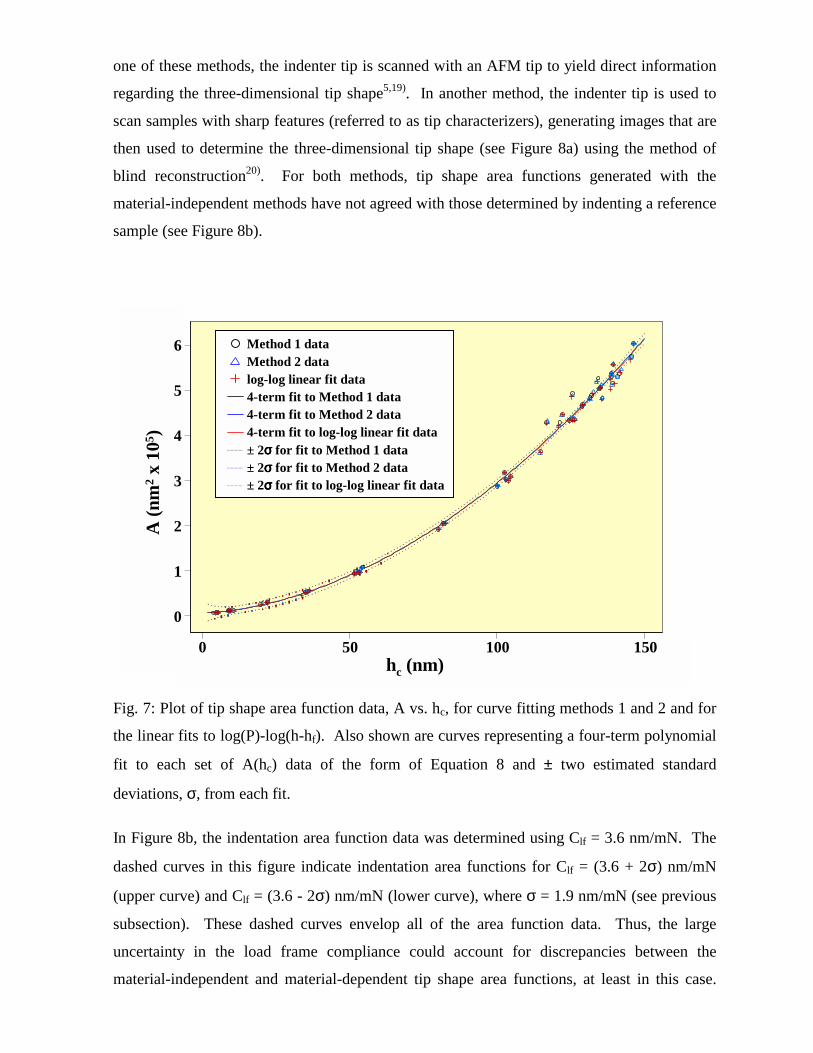
Fig. 7: Plot of tip shape area function data, A vs. hc, for curve fitting methods 1 and 2 and for

the linear fits to log(P)-log(h-hf). Also shown are curves representing a four-term polynomial

fit to each set of A(hc) data of the form of Equation 8 and ± two estimated standard

deviations, σ, from each fit.

In Figure 8b, the indentation area function data was determined using Clf = 3.6 nm/mN. The

dashed curves in this figure indicate indentation area functions for Clf = (3.6 + 2σ) nm/mN

(upper curve) and Clf = (3.6 - 2σ) nm/mN (lower curve), where σ = 1.9 nm/mN (see previous

subsection). These dashed curves envelop all of the area function data. Thus, the large

uncertainty in the load frame compliance could account for discrepancies between the

material-independent and material-dependent tip shape area functions, at least in this case.

0 50 100 150

c(h1, h1)

010

0000

2000

0030

0000

4000

0050

0000

6000

00

c(fit

+ q

t(0.9

75, d

f) * s

e.fit

, fit

- qt(0

.975

, df)

* se.

fit) 6

5

4

3

2

1

0

A (n

m2 x

105 )

0 50 100 150hc (nm)

4-term fit to Method 1 data4-term fit to Method 2 data4-term fit to log-log linear fit data± 2σσσσ for fit to Method 1 data± 2σσσσ for fit to Method 2 data± 2σσσσ for fit to log-log linear fit data

log-log linear fit dataMethod 2 dataMethod 1 data

Other uncertainties for the indentation method include those related to the detection of a true

zero in load and displacement, the load and displacement measurements themselves, and the

elastic properties of the sample and indenter materials. Differences between current analysis

methods based on elasticity theory and real material behavior, including correction factors β

and γ and the pile-up or sink-in of material around the tip-sample contact, can also be

significant sources of uncertainty. Uncertainties related to the material-independent AFM

methods include the finite sizes of either the AFM tip or the tip characterizer features, as well

as non-tip artifacts such as thermal drift, scanner nonlinearities, feedback-loop response time,

and slight deviations from orthogonality of the scanners. Also, the material-independent

methods do not account for deformation of the indenter tip, such that the derived tip shape is

perhaps a better representation of the actual tip shape than that determined via indentation due

to the inclusion of tip deformation. We are currently investigating the impact of these various

uncertainties on the total uncertainty of modulus measurements as determined from

indentation data.

While no complete uncertainty analysis has yet been performed regarding DSI methods, a few

interlaboratory and/or intersystem comparisons have been done, all of which resulted in poor

reproducibility in modulus measurements5,21,22). In one of these studies that included 8

laboratories and 6 different instrument types, measurements of E for fused silica (nominally E

= 72 GPa) ranged from (67.2 ± 0.4) GPa to (84 ± 3) GPa for Pmax = 100 mN and from (68.6 ±

0.3) GPa to (86.3 ± 0.3) GPa for Pmax = 10 mN 5). In another study with all data presumably

taken by the same researchers but using 6 combinations of 3 different DSI instruments and 5

different tips, reduced modulus values for single crystal tungsten ranged from approximately

(210 ± 50) GPa to (470 ± 60) GPa21). In addition, several of the instrument-tip combinations

yielded values of reduced modulus that increased with increasing contact depth while other

combinations yielded values that increased with decreasing contact depth. The large

uncertainties reported for these comparisons are likely due to uncertainties in the calibrations,

as has been discussed, as well as the repeatability of the measurements for each instrument22).

Finally, the use of ideal tip shapes in indentation calculations can create large uncertainties. In

our study, the opening angles, β, between the normal and the three faces of the two Berkovich

tip were calculated from the blind reconstruction data to range from approximately 66.5° to

67.5°. These measured values of β are not equal to either the original specification by

Berkovich of 65.033° degrees or the modified value of 65.3° specified by Oliver and Pharr.

However, the measured values are in agreement with values measured for a number of

Berkovich indenter tips using a metrological AFM that ranged between 65.7° and 67.4° 23).

(a)

(b)

Fig. 8: (a) Blind reconstruction of a Berkovich indentation tip; and (b) a plot of the area-depth

relationship for two Berkovich tips in which blind reconstruction results are compared to

results from an indentation tip-shape analysis. In (b), the indentation area function data was

determined using Clf = 3.6 nm/mN, and the dashed curves approximate indentation area

functions for Clf = (3.6 + 2σ) nm/mN (upper curve) and Clf = (3.6 - 2σ) nm/mN (lower curve),

where σ = 1.9 nm/mN.

0

100000

200000

300000

400000

500000

600000

700000

0 25 50 75 100 125 150

hc or distance from apex (nm)

Are

a (n

m2 )

A (tip 1)A (tip 2)BR (tip 1)BR (tip 2)

Artifact due tojoining solutions

Artifacts due to periodicity ofspike characterizer

x (nm)

y (nm)

z (nm)

0

2000

-2000-2000

2000

0

0

300

Besides the differences in opening angle, all conical and pyramidal indenter tips are likely to

have some sort of defect geometry, for example blunting, at the tip apex, as noted by Briscoe

and coworkers24-26). From our blind reconstruction results, the two Berkovich tips studied had

blunt tips, exhibiting pyramidal geometry only for vertical distances from the apex of 15 nm

or greater. Also, the opening angle measured close to the apex (i.e., approaching the blunt

region) was between 1° and 2° greater than the opening angle measured away the apex. As a

result of these deviations from ideality, the area values corresponding to a given contact depth

will be much different for real tips compared to an ideal tip, particularly for contact depths

less than 100 nm as are commonly encountered in nanoindentation.

Nanoindentation of Polymers

Nanoindentation Using DSI Systems

A number of problems exist with the current application of nanoindentation techniques to

polymeric materials using both DSI and SPM systems. In general, measurements of E using

DSI tend to increase with decreasing penetration depth, often referred to as an indentation size

effect. This artifact also appears to be a problem for indentation of polymers using DSI26).

Thus, either E(surface) > E(bulk) for a large number of materials, which seems unlikely, or

these trends result from increased uncertainties for shallow depth indents that are likely due to

tip defects near the apex and decreased signal-to-noise ratios at low load and displacement

levels. Also, values of E measured for polymers using DSI are significantly higher than

values measured using tensile testing or dynamic mechanical analysis (DMA). For example,

Lucas et al. reported E(DSI) = 1.2 GPa, E(tensile test) = 0.4 GPa, and E(DMA) = 0.5 GPa for

polytetrafluoroethylene (PTFE)4). For some studies, modulus values measured using DSI

have been compared to handbook or manufacturer values25). However, such comparisons can

often be misleading, because quoted values of E for many polymer systems can cover a large

range due to potential variations in microstructure, semicrystalline morphology, anisotropy,

molecular weight, crosslink density, etc. Thus, comparisons of modulus values are most

appropriate for polymer samples with identical chemistry, molecular weight, and processing

history.

To date, relatively few quasi-static indentation studies of polymers using DSI systems have

been published, largely because of the inadequacies of DSI systems and traditional analysis

methods as applied to measuring polymer properties. For example, the point taken as

representing initial contact (h = 0) generally corresponds to a significant applied load, such

that penetration of the indenter tip into a polymer could be significant relative to the

maximum displacement, hmax. Also, viscoelastic creep during unloading can dramatically

affect the slope of the unloading curve, leading to negative values of S in extreme cases28,29).

This creep effect has been shown through modeling to be related to a continued increase in

the contact radius during the initial portion of the unloading cycle30). Because of this affect,

power law fits will generally not be applicable to fitting the unloading response of polymers.

In fact, nonlinear power law fits (see Equation 1) often will not reach a convergent solution.

However, some commercial DSI system software will produce an answer based on the values

of the fitting parameters for the Nth iteration, where N is the total number of iterations

allowed by the fitting routine. Perhaps in realizing this problem, some researchers have

reverted to determining S using a linear approximation to the upper portion of the unloading

curve31), which assumes that the contact area remains constant for the initial unloading of the

material. However, this practice creates a dependence of S on the number of points used in the

linear fit, as discussed previously. Moreover, it ignores the cause of the deviation from power

law behavior, namely viscoelastic creep.

In our recent studies, a benzocyclobutene (BCB) polymer described in detail elsewhere20) was

indented with a DSI system using a Berkovich indenter tip. Load frame and tip shape

calibrations had been determined using traditional DSI methods, as discussed previously.

Additionally, blind reconstruction was used to generate a material-independent tip shape area

function20). Eleven load-penetration curves were performed with maximum loads of between

43 µN and 944 µN. Several different fitting routines were used to fit the unloading curves.

Power law fits using commercially available statistics software also did not converge. Power

law fits using the commercial DSI system software also did not converge for any of the data

sets, but values for S, hc, and E were output based on the values of the fitting parameters for

the final iteration. In Figure 9, the resulting curve fits are shown along with fits based on

linear fits to logarithmic data, neither of which were good representations of the unloading

curves. Note that for nonlinear power law fits, the power law exponents were all greater than

2, ranging from 2.2 to 2.7. Similar results were found by Briscoe and Sebastian. Using the

commercially available statistics software, a smooth spline fitting routine was then used,

which yielded excellent fits to the unloading data, as shown in Figure 10. Besides producing

a good fit to the data, this routine also produced a direct calculation of the first derivative of

the fitted curve corresponding to each data point, as shown in Figure 11 as a function of load.

For both the higher Pmax and lower Pmax indents shown in this figure, the slope of the upper

portion of the unloading curve does in fact remain relatively constant. Using the spline fitting

routine, however, yields values of S that are not dependent on a human judgement, such as

deciding on the number of points to include in a linear fit to the upper portion of the

unloading curve.

Fig. 9: An example of a DSI unloading curve for the BCB polymer and two corresponding

curve fits: (a) a power law fit using the commercial DSI system software that did not

converge and (b) a fit based on linear regression of logarithmic data.

Fig. 10: Examples of DSI unloading curves for the BCB polymer along with the smooth

spline curve fits for two different loads.

To compute values of E, values of S determined using the smooth spline fits were used to

calculate hc using Equation 5 with ε = 0.75. (Note that because power law fitting was not

used, this choice of ε here is somewhat arbitrary, i.e. it is not related to a power law exponent,

m such as in Table 1.) Those values of hc were then used to determine A from the tip area

function determined by indenting fused silica and that determined from blind

P (µ µµµ

N)

0

200

400

600

800

100 200 300 400 h (nm)

P (µ µµµ

N)

0

20

40

60

80

20 40 60 100 h (nm)

80100 200 300 400

Depth

020

040

060

080

0Lo

ad

20 40 60 80 100

Depth

020

4060

80Lo

ad

100 200 300 400

Depth

020

040

060

080

0

Load

P (µ µµµ

N)

0

200

400

600

800

100 200 300 400h (nm)

100 200 300 400

Depth

020

040

060

080

0Lo

ad

P (µ µµµ

N)

0

200

400

600

800

100 200 300 400h (nm)

reconstruction20). These two sets of modulus values are plotted in Figure 12a as a function of

hc. In both cases, these modulus values do not show any dependence on hc, in contrast to the

E values plotted in Figure 12b, which correspond to the non-convergent power law fits of the

DSI system software. Of course, the uncertainties in the modulus values of Figure 12 are still

under investigation, but the use of the non-convergent power law fits appears to be a possible

source of artificial increases in E with decreasing hc.

Fig. 11: Plots of the first derivative of the smooth spline curves in Figure 10 as a function of

load for two different loads.

Averaging the modulus values in Figure 12a, E = (3.5 ± 0.3) GPa using the blind

reconstruction area function, and E = (4.1 ± 0.2) GPa using the area function determined from

the indentation of fused silica. Both of these values are slightly higher than the room-

temperature tensile modulus of 2.9 GPa reported by the manufacturer. As discussed

previously, however, the occurrence of creep during unloading affects the determination of S

for polymeric materials. The indentations of the BCB polymer were performed using a load-

hold-unload cycle, so an effort was made to characterize the indentation creep response from

the 10 s portion of the cycle in which the load was held relatively constant at Pmax. The

change in tip displacement, h, with time, t, during the hold cycles of each indentation data set

was fit using a functional relationship of the form ∆h ~ (∆t)n, and the exponent, n, ranged

from 0.38 to 0.57.

To apply this crude characterize of creep response to the unloading curve, the convolution

integral relating the time-dependent strain, ε(t), to creep compliance, J(t), and the time rate of

change of stress, dσ/dt, was used32):

0 200 400 600 800

Load

02

46

810

pred

ict(s

sbcb

, Dep

th, 1

)$y

200 400 600 800P (µµµµN)

0

dP/d

h

0

2

4

6

8

10

0 20 40 60 80

Load

0.5

1.0

1.5

2.0

2.5

pred

ict(s

sbcb

, Dep

th, 1

)$y

20 40 60 80P (µµµµN)

0

dP/d

h0.5

1.0

1.5

2.0

2.5

( ) ( ) ττε τσ dtJt d

d∫ −= (11)

A uniform stress, σ(t) = P(t)/A(t), was assumed, ε(t) was taken to be related to ∆h/h, and J(t) =

k1tn was assumed, where n was determined from the creep response during the hold cycles. Of

course, the actual stress and strain distributions are highly non-uniform, and the hold portion

of the indentation tests deviates significantly from a conventional creep test. Also, contrary to

the Boltzmann Superposition Principle, the integral was not evaluated for all elements of the

loading history, but rather just the unloading portion of the indentation loading cycle. Finally,

whether indentation behavior of polymers follows the assumptions of linear viscoelasticity is

not clear. Thus, this viscoelastic analysis is only a rough estimate of the actual viscoelastic

behavior.

Using this approach, the estimated viscoelastic creep was removed from the unloading data

for each data set, and the smooth spline fits were again applied. The resulting values of S

were approximately 3 % to 6 % lower that the S values determined previously for the total

unloading curves. Using the blind reconstruction area function, the corresponding reductions

in E values were between 3 % and 5 %, resulting in an average value of E = (3.4 ± 0.3) GPa.

A more rigorous analytical or numerical approach might result in an even larger influence of

creep response on the values of E determined from indentation unloading curves. Another

potential effect could be that of hydrostatic stress, which has been shown to increase the

apparent modulus value of some polymers25). Research in these areas is currently being

pursued.

More recent applications of DSI to measuring polymer properties have focused on indentation

creep tests and also on dynamic indentation testing. Attempts have been made to model

indentation creep and stress relaxation data using standard linear solid models from which

values of E can be extracted from fits of the model predictions to the experimental data33-36).

Generally, these attempts have met with mixed success, most likely because the experimental

aspects do not conform to the assumptions of the analysis. For example, the modulus values

measured for instantaneous applications of load or displacement are often much lower than

expected, because a finite loading or displacement rate is used that does not simulate a step

function. In one case, the contact area was assumed to be constant during viscoelastic

creep36), which is not the case as discussed by Unertl30). The simplicity of the models used

compared to the actual polymer behavior and assumptions regarding stress and strain could

also lead to inaccuracies in the measured polymer properties.

(a)

(b)

Fig. 12: Plots of modulus measured for the BCB polymer from DSI as a function of contact

depth. The modulus values in (a) were determined using smooth spline fits and the two

different area functions indicated, while the modulus values in (b) were determined using

non-convergent power law fits and the indentation area functions.

Dynamic indentation testing has recently been developed for several indentation systems28,37).

This method is similar to dynamic mechanical analysis (DMA) in that a sinusoidal input is

applied and the output is monitored. For linear viscoelastic behavior, the output is also

sinusoidal but can lag the input signal. The in-phase components of stress and strain can be

used to determine the storage modulus, E', and the out-of-phase components are related to the

loss modulus, E". The ratio of these moduli, E"/E', is referred to as the loss tangent or tan δ.

0

1

2

3

4

5

0 50 100 150 200 250 300 350 400

hc (nm)

E (G

Pa)

0

1

2

3

4

5

0 50 100 150 200 250 300 350 400hc (nm)

E (G

Pa)

Using Blind Reconstruction Area FunctionUsing Indentation Area Function

In DMA, the input oscillation is normally displacement or strain and the output is load or

stress. In DSI, an oscillatory load is applied and the displacement is monitored28). The in-

phase component of the contact stiffness is then used to calculate E' and the out-of-phase

component is used to calculate E". The equations used for these calculates are analogous to

Equation 2, replacing S with either the in-phase or out-of-phase component of the contact

stiffness and replacing Er with either E' or E" 37). Unlike DMA, however, stress localization

and large strain gradients are associated with DSI, and the assumptions of linear

viscoelasticity have yet to be checked for dynamic indentation testing. Thus, caution should

be used in evaluating the resulting dynamic modulus values.

Nanoindentation Using SPM Systems

Three classes of systems can be categorized as SPM nanoindentation systems. In the first

type of system, AFM and DSI systems are integrated with the DSI transducer-tip assembly

mounted in place of the AFM cantilever probe, and indentation is controlled by the DSI

system. Contact mode scanning of the sample is also permitted using the DSI force signal in

the AFM feedback loop. However, the contact force applied during scanning is orders of

magnitude larger than typical AFM contact mode forces, and thus scanning with these

systems can severely deform and damage polymeric materials. Also, indentation tips

typically have larger tip radii compared to AFM cantilever tips, thus limiting the resolution of

resulting images. However, the ability to scan the surface to find a suitably smooth area or

particular surface features is often very important to nanoindentation studies. In terms of

indentation testing, the system acts as a traditional DSI system, as has been discussed at

length. In fact, this type of system was used in all of our studies of DSI that were previously

discussed.

The second type of instrumentation is the interfacial force microscope (IFM) developed at

Sandia National Laboratory by Houston and co-workers9). In terms of nanoindentation of

polymers, the IFM has a number of advantages over DSI systems. The main advantage is the

ability to indent using rigid displacement control, which allows tip penetration into the sample

to be controlled with subnanometer resolution and ensures that the load frame compliance is

zero, thus simplifying analysis11). This attribute results in much lower applied forces

compared to DSI such that true nanoscale spatial resolution can be achieved. Typically,

electrochemically etched tungsten wires have been used with the IFM, and the tip radii have

been determined using scanning electron microscopy to range from 70 nm to 500 nm10,11).

Penetration of the tip into the sample is normally much less that the probe tip radius, and thus

a Hertzian analysis, which is a special case of Equation 1 with m = 1.5 and α = 4Er√R/3, can

be used to evaluate the indentation response and calculate sample modulus. In many cases, no

hysteresis is observed between loading and unloading curves, indicating pure elastic

deformation, such that either the loading curve or unloading curve can be analyzed11,38).

Reasonable modulus measurements for polymers using the IFM have been achieved, although

similar questions regarding uncertainties as those discussed for DSI remain. Also, in one

study, the IFM was used to perform an indentation stress relaxation experiment on PTFE, in

which a 15 % decrease in the applied load was observed in less than 3 s of the application of a

constant displacement39). The current scanning capabilities of the IFM, which include only

contact mode, are limited compared to the AFM, but the contact mode scanning forces are

significantly less than the integrated DSI-AFM system. Also because of the larger tip radii,

image resolution for the IFM is not as good as for AFM.

Quantitative indentation methods have also been developed recently using AFM cantilever

probes that can also be used for imaging purposes6). Original attempts to use the AFM as an

indentation device were done using a privately built system designed specifically for

nanoindentation and having limited scanning capabilities40). More recent efforts, particularly

those focussed on indenting polymers and biological materials, have utilized commercial

AFM systems and commercial cantilever probes41-46). The advantage of using commercial

systems is the potential to combine nanoindentation testing with robust, high resolution

imaging capabilities. In fact, through recent developments by one AFM vendor, some

commercial AFM systems offer the capability to switch back and forth between tapping mode

imaging and indentation mode. However, because commercial AFM systems have not been

specifically designed for indentation testing, a number of instrumental uncertainties severely

limit their uses as nanoindenters7). Despite these limitations, successful nanoindentation

studies of polymers have been reported. These successes include studies of a wide variety of

commercial polymeric materials42), interphases in fiber-reinforce polymer materials8),

crystalline regions in polyethylene and polyethylene blends46), aerogel powder particles45),

polymer thin films43,44), and differences between the surface and interior of a

polydimethylsiloxane6). In the AFM indentation studies performed to date, however, the

measurements of modulus have been either relative measurements or measurements with

large uncertainties due to the use of idealized tip shapes and nominal spring constants.

Further, Hertzian or Sneddon models have been utilized in all of these studies, such that

viscoelastic behavior has been ignored.

In our recent studies, the BCB polymer used in the previously discussed DSI study was

indented using a diamond-tipped stainless steel AFM cantilever probe. The spring constant,

kc = (120 ± 10) N/m, was measured by the manufacturer using a technique in which the force

applied to a mica sample is measured by a digital microbalance as a function of measured tip

deflection. Blind reconstruction was then used to estimate the tip shape area function as

described elsewhere20). Load frame compliance for the AFM cantilever was performed by

pushing on a sapphire sample. In this case, because the sample contact stiffness is much

larger than the probe spring constant, no tip penetration occurs and the measured force-

displacement response is characteristic of the given AFM probe and the particular operating

conditions. The probe response can be removed from the force-displacement responses

measured on the polymer sample so that only the force-penetration response remains6-8).

Eight load levels ranging from 1.4 µN to 13.7 µN were used to indent the BCB sample. For

each load level, 10 force curves were obtained on a smooth sapphire sample, five directly

before and five directly after indenting the BCB sample, using the same probe and operating

conditions. As with the DSI study of the BCB polymer, smooth spline curves were fit to the

unloading curves after unsuccessful attempts to get good fits using nonlinear power law fits

and linear fits to logarithmic data.

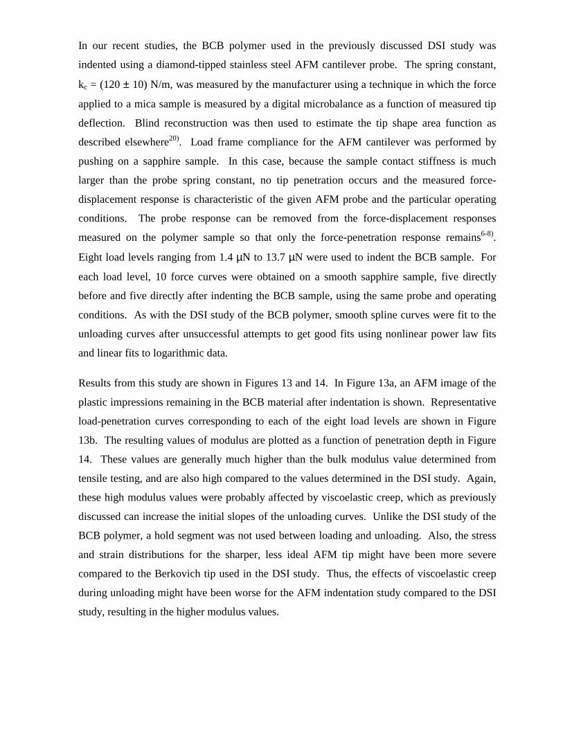
Results from this study are shown in Figures 13 and 14. In Figure 13a, an AFM image of the

plastic impressions remaining in the BCB material after indentation is shown. Representative

load-penetration curves corresponding to each of the eight load levels are shown in Figure

13b. The resulting values of modulus are plotted as a function of penetration depth in Figure

14. These values are generally much higher than the bulk modulus value determined from

tensile testing, and are also high compared to the values determined in the DSI study. Again,

these high modulus values were probably affected by viscoelastic creep, which as previously

discussed can increase the initial slopes of the unloading curves. Unlike the DSI study of the

BCB polymer, a hold segment was not used between loading and unloading. Also, the stress

and strain distributions for the sharper, less ideal AFM tip might have been more severe

compared to the Berkovich tip used in the DSI study. Thus, the effects of viscoelastic creep

during unloading might have been worse for the AFM indentation study compared to the DSI

study, resulting in the higher modulus values.

(a)

(b)

Fig. 13: (a) AFM image of the plastic impressions remaining in the BCB material after

indentation (height scale is 0 nm to 20 nm from black to white), and (b) representative load-

penetration curves corresponding to each of the eight load levels.

Conclusions

In this paper, the use of depth-sensing indentation methods to measure the elastic modulus of

polymeric materials was reviewed. Included in this review were discussions of traditional

analyses of load-penetration data, the use of depth-sensing indenters and scanning probe

microscopes to measure the nanoscale mechanical response of polymers, and the associated

uncertainties and limitations of various nanoscale indentation measurements. The application

of these methods to polymers often leads to inaccurate measurements of elastic modulus. For

quasi-static indentation, viscoelastic behavior affects the shape of the unloading curve,

resulting in modulus values that are high relative to bulk measurements. Attempts to

characterize creep behavior during indentation experiments suffer from system limitations

0

2000

4000

6000

8000

10000

12000

14000

16000

0 20 40 60 80 100

Indentation Depth (nm)

Loa

d (n

N)

(e.g., relatively slow rates of loading compared to the necessary step loading) and potentially

inappropriate assumptions regarding the stress and strain distributions under indentation

loads. While additional complications might arise, dynamic indentation testing has the

potential to alleviate many of the problems associated with quasi-static indentation testing.

However, a rigorous analysis of dynamic indentation behavior of polymers, particularly with

regard to whether or not linear viscoelasticity holds, has not been reported. Advancement of

these methods toward quantitative characterization of polymer properties will require

material-independent calibration procedures, polymer reference materials, advances in

instrumentation, and new testing and analysis procedures that account for polymer rheological

behavior.

Fig. 14: Plot of modulus measured for the BCB polymer from indentation with an AFM

cantilever as a function of contact depth.

References

1. W. C. Oliver, G. M. Pharr, J. Mater. Res. 7(6), 1564 (1992). 2. S. G. Corcoran, R. J. Colton, E. T. Lilleodden, W. W. Gerberich, Phys. Rev. B 55(24), 57

(1997). 3. M. F. Doerner, W. D. Nix, J. Mater. Res. 1(4), 601 (1986). 4. B. N. Lucas, in: Thin-Films -- Stresses and Mechanical Properties VII 505, Materials

Research Society, Pittsburgh, PA, 1998, p. 97. 5. N. M. Jennett, J. Meneve, in: Fundamentals of Nanoindentation and Nanotribology 522,

Materials Research Society, Pittsburgh, PA, 1998, p. 239. 6. M. R. VanLandingham, S. H. McKnight, G. R. Palmese, J. R. Elings, X. Huang, T. A.

Bogetti, R. F. Eduljee, J. W. Gillespie Jr., J. Adhesion 64(1-4), 31 (1997). 7. M. R. VanLandingham, Microscopy Today, Issue No. 97-10, pp. 12-15, 1997.

0

1

2

3

4

5

6

7

0 20 40 60 80 100hc (nm)

E (G

Pa)

8. M. R. VanLandingham, R. R. Dagastine, R. F. Eduljee, R. L. McCullough, J. W. Gillespie, Jr., Composites−A 30(1), 75 (1999).

9. S. A. Joyce, J. E. Houston, Rev. Sci. Instrum. 62(3), 710 (1991). 10. S. A. Joyce, R. C. Thomas, J. E. Houston, T. A. Michalske, R. M. Crooks, Phys. Rev. Lett.

68(18), 2790 (1992). 11. J. D. Kiely, J. E. Houston, Phys. Rev. B 57(19), 12588 (1998). 12. I. N. Sneddon, Int. J. Engng. Sci. 3, 47 (1965). 13. R. B. King, Int. J. Solids Structures 23(12), 1657 (1987). 14. J. C. Hay, A. Bolshakov, G. M. Pharr, J. Mater. Res. 14(6), 2296 (1999). 15. J. L. Hay, in: Proceedings of the SEM IX International Congress on Experimental

Mechanics, Society for Experimental Mechanics, Bethel, CT, 2000, p.665. 16. J. Neter, M. H. Kutner, C. J. Nachtsheim, W. Wasserman, Applied Linear Statistical

Models, Irwin, Chicago, IL, 1974, p. 97. 17. B. Bhushan, A. V. Kulkarni, W. Banin, J. T. Wyrobek, Phil. Mag. A 74(5), 1117 (1996). 18. Y.-T. Cheng, C.-M. Cheng, Int. J. Solids Structures 36, 1231 (1999). 19. J. L. Meneve, J. F. Smith, N. M. Jennett, S. R. J. Saunders, Appl. Surf. Sci. 100/101, 64

(1998). 20. M. R. VanLandingham, J. S. Villarrubia, G. F. Meyers, in: Proceedings of the SEM IX

International Congress on Experimental Mechanics, Society for Engineering Mechanics, Bethel, CT, 2000, p. 912.

21. W. W. Gerberich, W. Yu, D. Kramer, A. Strojny, D. Bahr, E. Lilleodden, J. Nelson, J. Mater. Res. 13(2), 421 (1998).

22. S. R. J. Saunders, G. Shafirstein, N. M. Jennett, S. Osgerby, J. Meneve, J. F. Smith, H. Vetters, J. Haupt, Phil. Mag. A 74(5), 1129 (1996).

23. N. M. Jennett, personal communication (June 1, 2000). 24. B. J. Briscoe, K. S. Sebastian, M. J. Adams, J. Phys. D: Appl. Phys. 27, 1156 (1994). 25. B. J. Briscoe, K. S. Sebastian, Proc. Roy. Soc. Lond. A 452, 439 (1996). 26. B. J. Briscoe, K. S. Sebastian, S. K. Sinha, Philosophical Magazine A 74(5), 1159 (1996). 27. B. J. Briscoe, L. Fiori, E. Pelillo, J. Phys. D: Appl. Phys. 31, 2395 (1998). 28. B. N. Lucas, W. C. Oliver, A. C. Ramamurthy, in: ANTEC Conference Proceedings 3,

Society of Plastics Engineers, Brookfield, CT, 1997, p. 3445. 29. I. Adhihetty, J. Hay, W. Chen, P. Padmanabhan, in: Fundamentals of Nanoindentation

and Nanotribology 522, Materials Research Society, Pittsburgh, PA, 1998, p. 317. 30. W. N Unertl, ACS Polym. Preprints 39(2), 1232 (1998). 31. A. Strojny, X. Xia, A. Tsou, W. W. Gerberich, J. Adhesion Sci. Technol. 12(12), 1299

(1998). 32. I. M. Ward, Mechanical Properties of Solid Polymers, Wiley-Interscience, New York

1971, p.85. 33. L. Cheng, X. Xia, W. Yu, L. E. Scriven, W. W. Gerberich, J. Polym. Sci: Part B: Polym.

Phys. 38, 10 (2000). 34. L. Cheng, L. E. Scriven, W. W. Gerberich, in: Fundamentals of Nanoindentation and

Nanotribology 522, Materials Research Society, Pittsburgh, PA, 1998, p. 193. 35. A. Strojny, W. W. Gerberich, in: Fundamentals of Nanoindentation and Nanotribology

522, Materials Research Society, Pittsburgh, PA, 1998, p. 159. 36. K. B. Yoder, S. Ahuja, K. T. Dihn, D. A. Crowson, S. G. Corcoran, L. Cheng, W. W.

Gerberich, in: Fundamentals of Nanoindentation and Nanotribology 522, Materials Research Society, Pittsburgh, PA, 1998, p. 205.

37. S. A. Syed Asif, J. B. Pethica, in: Thin-Films -- Stresses and Mechanical Properties VII 505, Materials Research Society, Pittsburgh, PA, 1998, p. 103.

38. S. K. Khanna, K. Paruchuri, P. Ranganthan, R. M. Winter, in: Proceedings of the SEM IX International Congress on Experimental Mechanics, Society for Engineering Mechanics, Bethel, CT, 2000, p. 916.

39. A. J. Howard, R. R. Rye, J. E. Houston, J. Appl. Phys. 79(4), 1885 (1996). 40. N. A. Burnham, R. J. Colton, J. Vac. Sci. Technol. A 7(4), 2906 (1989). 41. A. L. Weisenhorn, M. Khorsandi, S. Kasas, V. Gotzos, H.-J. Butt, Nanotechnol. 4, 106

(1993). 42. S. A. Chizhik, Z. Huang, V. V. Gorbunov, N. K. Myshkin, V. V. Tsukruk, Langmuir 14,

2606 (1998). 43. J. Xu, J. Hooker, I. Adhihetty, P. Padmanabhan, W. Chen, in: Fundamentals of

Nanoindentation and Nanotribology 522, Materials Research Society, Pittsburgh, PA, 1998, p. 217.

44. J. Domke, M. Radmacher, Langmuir 14, 3320 (1998). 45. R. W. Stark, T. Drobek, M. Weth, J. Fricke, W. M. Heckl, Ultramicrosc. 75, 161 (1998). 46. M. S. Bischel, M. R. VanLandingham, R. F. Eduljee, J. W. Gillespie Jr., J. M. Schultz, J.

Mater. Sci. 35, 221 (2000).