An Experimental Study on Coupling DCMD with SGSP through Its Wall Heat Exchanger

Khaled Nakoa, RMIT University, Australia Abhijit Date, RMIT University, Australia

Aliakbar Akbarzadeh, RMIT University, Australia

The North American Conference on Sustainability, Energy & the Environment 2014 Official Conference Proceedings

Abstract The interest of using solar powered membrane distillation systems for desalination is growing worldwide due to the membrane distillation (MD) attractive features. This study experimentally investigates utilization of direct contact membrane distillation (DCMD) coupled to a salt-gradient solar pond (SGSP) for sustainable freshwater production and reduction of brine footprint on the environment. A model for heat and mass flux in the DCMD module and a thermal model for an SGSP are developed and coupled to evaluate the feasibility of freshwater production. Experiments are conducted at RMIT University renewable energy laboratory using SGSP wall heat exchanger. The feed stream of 1.3% salinity is heated up by the wall heat exchanger and circulated through MD module then injected back to an evaporation pond. Also, a heat recovery system (Heat Exchanger) is used to back up heat from the outlet brine stream of DCMD and use it as preheating for inlet feed stream flow. Results are compared and shown that if the flow is laminar, the connecting DCMD module to the SGSP could induce marked concentration and temperature polarisation phenomena that reduce fluxes. Therefor turbulence has to be created in the feed stream to reduce polarisations and the brine is recirculated after passing through the heat exchanger to reduce the environmental footprint. Keywords: Solar Membrane Distillation, Solar desalination, DCMD & SGSP desalination, Membrane mass flux.

iafor The International Academic Forum

www.iafor.org

1. Introduction: Since 1950, the growth of global demand for freshwater has increased dramatically and approximately doubled every 15 years. This growth has reached a point where today existing freshwater resources are under great stress, and it has become both more difficult and more expensive to develop new freshwater resources. One particular issue is that a large proportion of the world's population (approximately 70 %) settles in coastal zones [1]. The current mean population density at coastlines is almost 100 ℎ𝑎𝑏/𝑘𝑚!, and it is over 2.5 times the global average and embraces 45% of the global population [2]. Many of these coastal regions rely on underground aquifers for a substantial portion of their freshwater supply. Specifically, if an aquifer is overdrawn, it can be contaminated by an influx of seawater or salts and, therefore, requires a treatment or purification. About 450 million people in 29 countries face severe water shortage; about 20% more water than is now available will be needed to feed the additional three billion people by 2025 [3]. Furthermore, the world health organization (WHO) reported that 20% of the world population already has inadequate drinkable water. Even though the two third of the planet is covered with water, 99.3 % of this water either has high salinity or not accessible ( Ice caps ) [4]. So the combined effects of increasing freshwater demand, population growth and seawater intrusion into coastal aquifers are stimulating the need for desalination. The desalination is a process of removing salts and other minerals from a saline water solution producing fresh water, which is suitable for human consumption, agriculture and industrial use. The desalination system usually consists of three main parts; water source which may be brackish or sea water, desalination unit and energy source which is playing the key role in evaluating the desalination plant performance. The aim of producing water at less energy consumption has led to promising solution which is solar desalination as most of countries have unlimited seawater resources and also a good level of solar energy. However, the strong potential of solar energy to seawater desalination process is not yet developed at the commercial level [5]. Solar desalination is an environmental friendly and cost saving process competitive with other conventional desalination techniques [6]. Also, the utilization of low-temperature membrane distillation (MD) coupled to a renewable energy source can be sustainable solution for the water and energy scarcity. Membrane distillation is a process working on the principle of phase change or vapour-liquid interface that has the capability to grow into a viable tool for solar water desalination. Direct contact membrane distillation (DCMD) is a configuration of MD where warmer feed solution is in direct contact with one side of a microporous hydrophobic membrane and cold water (permeate) is in direct contact with the opposite side of the membrane (Fig. 1) [7].

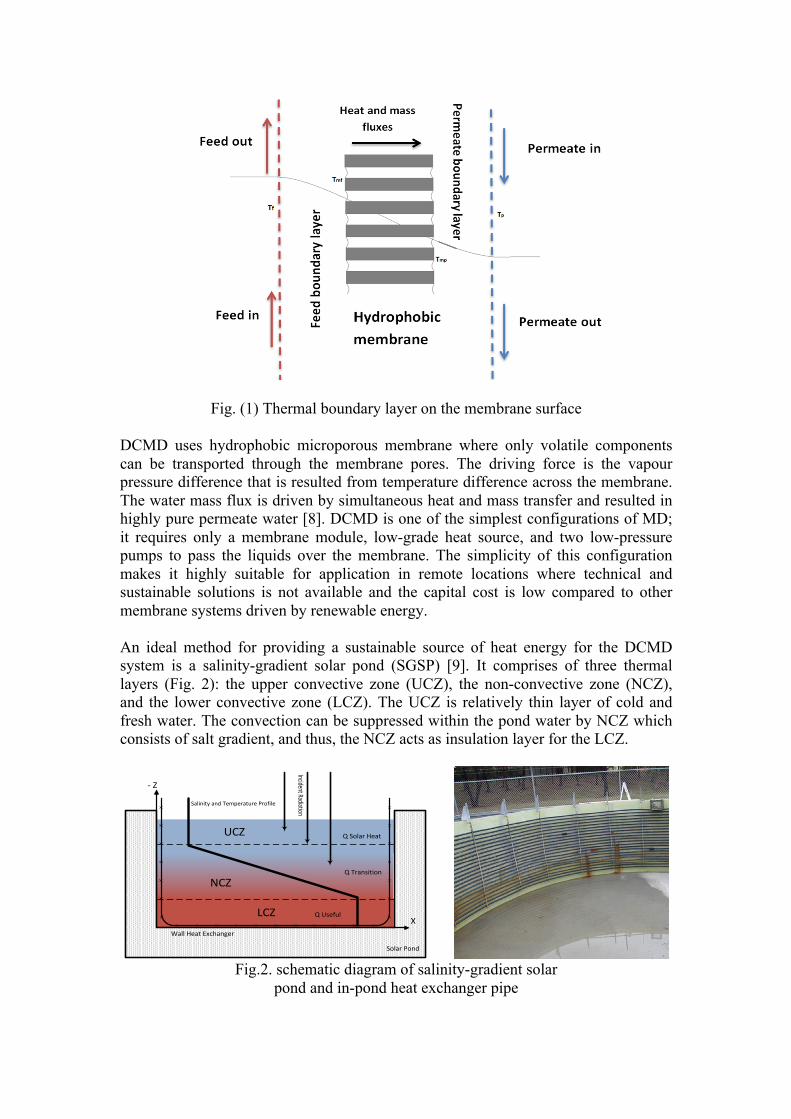
Fig. (1) Thermal boundary layer on the membrane surface

DCMD uses hydrophobic microporous membrane where only volatile components can be transported through the membrane pores. The driving force is the vapour pressure difference that is resulted from temperature difference across the membrane. The water mass flux is driven by simultaneous heat and mass transfer and resulted in highly pure permeate water [8]. DCMD is one of the simplest configurations of MD; it requires only a membrane module, low-grade heat source, and two low-pressure pumps to pass the liquids over the membrane. The simplicity of this configuration makes it highly suitable for application in remote locations where technical and sustainable solutions is not available and the capital cost is low compared to other membrane systems driven by renewable energy. An ideal method for providing a sustainable source of heat energy for the DCMD system is a salinity-gradient solar pond (SGSP) [9]. It comprises of three thermal layers (Fig. 2): the upper convective zone (UCZ), the non-convective zone (NCZ), and the lower convective zone (LCZ). The UCZ is relatively thin layer of cold and fresh water. The convection can be suppressed within the pond water by NCZ which consists of salt gradient, and thus, the NCZ acts as insulation layer for the LCZ.

Solar  Pond

Wall  Heat  Exchanger  

Salinity  and  Temperature  Profile

Incident  Radiation

UCZ

NCZ

LCZ

Q  Solar  Heat

Q  Transition

Q  Useful

-­‐  Z

X

Fig.2. schematic diagram of salinity-gradient solar

pond and in-pond heat exchanger pipe

At the LCZ layer, the salt concentration and temperature have the highest values and working as a heat energy storage. In fact, the solar radiation penetrates the pond’s upper layers then passes through NCZ then reaches the LCZ and heats up the highly concentrated brine. The LCZ can reach temperatures greater than 90°C and the useful heat can be used directly for low-temperature thermal applications. SGSP has been used previously to provide heat energy for desalination and it was found to be amongst the most cost-effective alternative energy systems for desalinating water process [10]. In 1987, the most notable work began with solar pond of 3000 m2 in El Paso, Texas, USA. At this site, a small multi-effect, multi-stage flash distillation unit with a brine concentration and recovery system, and a 2.94 m2 air-gap MD (AGMD) unit were tested in conjunction with the solar pond to evaluate the performance and the reliability of this technology. These desalination units were selected as they are usually operated with low grade temperature source and therefore, are more suitable to operate with the thermal energy generated by solar ponds [11]. The multieffect, multi-stage unit produced an average water amount of 3.3 L/min, which was comparable to a water production of 1.6*10-3 m3 per day per m2 of SGSP. However, this unit required large amount of electricity to operate the system at approximately 30 kPa and a temperature higher than 60°C to start the desalination process. Using AGMD, a maximum flux of 6.7 (L/m2/hr) and a water production of 0.158*103 m3 per day per m2 of SGSP, was achieved [11]. This maximum water production was obtained with a temperature difference of 41 C across the membrane module. Moreover, the water production significantly decreased when the system operates at lower temperature difference across the membrane. Most commercial MSF units operate with a top brine temperature of 90 – 110°C heated by steam while the solar pond operates in the range of 30 – 95 °C. Therefore, in solar pond assisted MSF systems, the first stage of the MSF heat exchangers is changed to liquid-liquid heat exchanger instead of steam–liquid heat exchanger. Some selected solar pond assisted desalination plant research studies are listed in Table 1.

Table (1) Selected SGSP & MD desalination systems

Ref. Mod./exp. Location / Radiation W/m2

SGSP size m2

Desalination method

Capacity Cost ($/M3)

[12] Model Tripoli, Libya 350

70000 MSF 1238 - 1570 m3/day

1.8

[13] Model Dead sea/Jordan 200-500

3000 MSF 6 m3/day Na

[14] Experiment

Ancona, Italy

625 MED 30 m3/day Na

[11] Model Walker, NV, USA

Na DCMD 2.7*10-3 m3/ day/m2 of SGSP

Na

[10] Model Gabès, Tunisia/ 588 - 1085

Na VMD 71 L/hr/m2 Na

In fact, MD desalination requires thermal and mechanical energy; therefore it is similar to the solar assisted MSF/MED process, which could use low grade heat from solar pond, electricity from a PV system or the power grid. Regarding MD energy consumption and cost, researchers are not completely agreed about its preferability. Some consider that MD from an energy consumption perspective is unfavourable when compared with MED and MSF because of the additional resistance to mass transport and reduced thermal efficiency (due to heat conductivity losses) [8]. In contrast, others claim that comparing to MSF plants, the MD energy consumption is similar but the pumping power is less [15]. However, by using new materials and optimizing the MD configuration, the temperature and concentration polarization salt solution can be simultaneously reduced in the DCMD [16], which might potentially reduce the cost. In addition, MD uses robust and cheap membranes, which means that MD could save on the usage of chemical and the saline water pretreatment costs compared to RO [8]. Some selected solar assisted MD seawater desalination systems can be seen in Table 1, in which most solar assisted MD systems operates at temperatures less than 80°C. However, modelling results have shown that combining solar collectors with the MD system could achieve a higher membrane permeate flux [17]. Although, there are many cost estimation reports about MD desalination, there are only a few on solar MD desalination costs. Banat et al. estimated the produced water cost by $15/m3 for a 100 l/d system using a 10 m2 membrane and 5.73 m2 flat panel collectors (FPC). Also, the cost was $18/m3 for a 500 l/day system using FPC–PV driven MD, 40 m2 membranes and 72 m2 FPC [18]. The study showed that by increasing the plant life time and the reliability, the cost could be further reduced. Overall, solar assisted MD is still under development stage. Reports on novel processes, experimentally confirmed modelling and pilot plant evaluations continue to appear in the literature [5]. MD has some disadvantage compared to MED and MSF of additional resistance to mass transport by the membrane. However, this disadvantage can be overcome since the MD materials develop lower cost and/or by using more area for heat and mass transfer. In addition, it could be used for highly concentrated saline water treatment or high recovery, that RO could not handle, which normally require high energy consumption. 2. MD theoretical approach: In MD, the driving force for water vapour transfer through the membrane pores is the temperature difference between the feed/membrane interface temperature (𝑇!") and the permeate/membrane interface temperature (𝑇!"). This generates a vapour pressure difference between both membrane sides which forces the vapour molecules to travel through the membrane pores and condensate at cold membrane side. 2.1 Flow Mechanisms: There are three basic mechanisms of mass flow inside the membrane wall, which are Knudsen diffusion, Poiseuille flow and molecular diffusion. In Knudsen diffusion, the pore size is too small, and the collision between molecules can be neglected. Furthermore, the collision between sphere molecules and the internal walls of the membrane is the dominant mass transport form. Molecular diffusion occurs if the pore size is big comparing to the mean free path of molecules and they move corresponding to each other. The flow is considered Poiseuille (viscous flow) if the

molecules act as continuous fluid inside the membrane pores. In general, different mechanisms occur simultaneously (Knudsen, Poiseuille and Molecular diffusion) inside the membrane if the pore size is less than 0.5 µm [19]. 2.2 Knudsen number: It is a governing quantity of the flow mechanism inside the membrane pores which is the ratio between the mean free path of the transported molecules and the pore size of the membrane. It is as follow:

𝑘𝑛 = !! (1)

S is the mean free path of the transferred gas molecule and d is the mean pore diameter of the membrane. S is calculated from:

𝑆 = !!!!!"!!!

(2) The pore sizes of the most membranes are in the range of 0.2 -1.0 µm. The mean free path of water vapour is 0.11 µm at feed temperature of 60°c. Therefor 𝑘𝑛   is the range of 0.11-0.55[19]. The different flow mechanisms inside the membrane pores can be identified by Knudsen number (𝑘𝑛): 𝑘𝑛   < 0.01 Molecular diffusion 0.01 < 𝑘𝑛 < 1   Knudsen-molecular diffusion transition mechanism 𝑘𝑛 > 1 Knudsen mechanism 2.3 Mass Flux (J): As shown in figure (1), vapour in transferring from feed side of the membrane to the permeate side by pressure difference force which is resulted from the temperature difference between two sides. The mass transfer may be written as a linear function of the vapour pressure difference across the membrane, given by:

𝐽 = 𝐶! 𝑃! − 𝑃!                            𝑘𝑔/𝑚!/𝑠𝑒𝑐 (3) Where 𝐽 is the mass flux, 𝐶! is the membrane distillation coefficient, and 𝑃!,𝑃! are the partial pressure of water vapour evaluated at the membrane surface temperatures      𝑇!  , 𝑇!. 𝐶! for Knudsen flow mechanisms:

 𝐶!! =!!"!!"

!!!"#

!! (4)

𝐶! for molecular diffusion 𝐶!! =

!!"

!"!!

!!"

(5) 𝐶! for Knudsen-molecular diffusion transition mechanism:

𝐶!! =!!!"!"

!"#!!

!! + !"

!!!!"

!"!

!!

(6)

D is the diffusion coefficient of the vapour in the air. 𝑃 is the pressure at 𝑇 and can be found using Antoine equation:

𝑃� = exp(  23.238− !"#$!!!"

 ) (7a) (𝑇) is the average membrane temperature. The vapour pressure decreases with increasing of feed water salinity according to Raoult’s law as follow [4]: 𝑃!! = 1− 𝑥! 𝑃! (7b) Where xc is the weight fraction of salt in water. 2.4 Heat Flux (q): The heat transfer models of MD can be summarized as follows:

• Convective heat transfer from the feed side to the membrane surface boundary layer:

𝑞! = ℎ! 𝑇! − 𝑇!" (8) Where qf is the feed heat flux (W/m2) and ℎ! is the heat transfer coefficient (W/m2.K).

• Heat flux through the membrane which includes conduction heat flux through the solid material of the membrane 𝑘!

!"!"

, and the latent heat transfer as a conviction by water vapour through the pores 𝐽𝐻!:

𝑞! = 𝐽𝐻! + 𝑘!!"!"

(9)

𝐻! is the vaporisation enthalpy of water evaluated at the mean temperature !!"!!!"

! ,

and the second term is the conduction heat loss through the membrane material. Finally, heat is transferred through the permeate boundary layer to the permeate water by convection.

𝑞! = ℎ!(𝑇!" − 𝑇!) (10) At steady state:

𝑞! = 𝑞! = 𝑞! (11) The overall heat transfer coefficient can be determined by:

𝑈 = !!!+ !

!!!!

! !!!!!"!!!"

+ !!!

!!

(12)

The rate of total heat transferred through the membrane is:

   𝑞! = 𝑈  (𝑇!  _  𝑇!) (13) The feed flow energy balance is:

𝑞! = 𝑚!  𝑐!(𝑇!,!" − 𝑇!,!"#) (14) The thermal efficiency of the MD system is:

𝐸! % =   !!!!!!

∗ 100 (15)

The thermal efficiency is the ratio between the water heat energy consumption to generate vapour and the total heat energy supplied to the system. Whereas, heat conduction through membrane solid, is considered heat loss and it should be minimised. To be more adequate, the efficiency should include both thermal and electrical energy (pumps) thus GOR (Gained Output Ratio) can define it as:

𝐺𝑂𝑅 = !!!!!!!!!

(16) To determine heat transfer coefficients of the boundary layers at both membrane sides the average bulk temperature of feed side

!!!!!"

! , and at permeate side !!"!!!

! of the

membrane should be used. Graetz-Leveque correlation is recommended [20]:

𝑁! = 1.86   𝑅!𝑃!!!!

!.!!                                            𝑑! =

!!!!!

(17) This correlation can be used for laminar flow (𝑅𝑒   <  2100). In contrast, next correlation can be applied for turbulent flow(2500 < 𝑅! < 1.25 ∗10!  𝑎𝑛𝑑  0.6 < 𝑃! < 100).

𝑁! = 0.023  𝑅𝑒!.!𝑃𝑟!                                (18) Where n is equal to 0.4 for heating, and 0.3 for cooling [21]. The dimensionless groups, Nusselt number (𝑁𝑢), Reynolds number (𝑅𝑒) and Prandtl number (𝑃!) can be calculated straightforwardly using the available physical data of feed and permeate fluid. At both sides of the membrane where the vapour-liquid interface takes place; there is a thermal boundary layer which its temperature differs from the bulk stream. This difference is described as temperature polarisation coefficient (TPC).

𝑇𝑃𝐶 = !!"!!!"

!!!!! (19)

The iterative method by a computer software (MATLAP®) is applied to predict 𝑇!" and  𝑇!". By entering the geometry and fluid properties, the software calculates the boundary heat transfer coefficients those to be used with other correlations. Then it uses the values of  𝑇!" and 𝑇!"    which are initially assumed equal to the bulk temperature 𝑇!  𝑎𝑛𝑑  𝑇! respectively, to determine the new values of 𝑇!"  𝑎𝑛𝑑  𝑇!" by a number of iterations. Equations (21) and (22) are used to predict both temperatures. Once the surface temperatures 𝑇!" and 𝑇!"    are determined, the software calculates the rest of required parameters. Please refer to the appendix (A) as an example of those values. To determine the evaporation latent heat: 𝐻! is evaluated at 𝑇                          𝑇 = !!"!!!"

!     (20)

From heat balance through the membrane and boundary layers: 𝑇!" =

!! !!! !! !! !! !!!!!!!!!!!!!!(!!!! !!)

(21)

𝑇!" =!! !!! !! !! !! !!!!!!!!!

!!!!!(!!!! !!) (22)

Where 3. SGSP heat extraction: A salinity gradient solar pond of 50 m2 located at RMIT Bundoora east campus, Australia, in renewable energy laboratory field was used to connect with DCMD module to work as heat energy source. The pond was designed with a depth of 2.05 m. The bottom storage zone was designed to be 0.56 m thick, the gradient zone 1.34 m thick and the top convective zone 0.15 m thick. The rate of heat extraction from this pond through its wall heat exchanger is given by:

𝑄 =  𝐴! .𝑈. 𝐿𝑀𝑇𝐷 (24) Where Ao is the external surface area of the heat exchanger pipe, U is the overall heat transfer coefficient based on the external surface area (in W/m2 °C) and LMTD is given by

𝐿𝑀𝑇𝐷 =   [!!!!!]!"[(!!"!!!)/(!!"!!!)]

(25)

Where Ti, To and Tpo are the temperature of the inlet and outlet of the wall heat exchanger and solar pond, respectively. The rate of extracted thermal energy is given by:

𝑄 =  𝑚! ∗ 𝐶! ∗  (𝑇!" − 𝑇!") (26) Where 𝑚 is the mass flow rate (in kg/s) and Cp is the specific heat of the circulating saline water (in J/kg °C) through the pipe. The solar pond efficiency can then be calculated by:

                         𝑒!" =!∗!!∗ !!"!!!"

!∗!!"   (27)

Where G is the solar radiation at the surface of the pond (in W/m2) and Asp is the area of solar pond. Therefore, the overall heat transfer coefficient of the in-pond heat exchanger pipe can be found from equation (24).

𝑈 = !!!∗!"#$

(28) 4. Water production and heat energy recovery: After DCMD operational parameters were selected (e.g., feed and permeate velocity, partial pressure of air entrapped in the pores) and the SGSP specifications (e.g., surface area, thickness of each zone) were determined, the performance of the coupled DCMD/SGSP system was evaluated. Specifically, heat extracted from the SGSP,

ℎ! = !!!!   (23)

water mass flux, and energy required for permeate water production through the membrane were determined. The necessary membrane surface area to use all the energy collected in the SGSP was also determined. In addition, the required membrane area ADCMD (m2) for the DCMD module, when the heat extracted from the SGSP is used without losses, can be found by equating the energy stored in the SGSP with the energy consumed by the DCMD module. Thus:

(𝐴!" ∗ 𝑞!"#) ∗ 𝑒!" = 𝐴!"#! ∗ 𝑞! (29) Where ASP (m2) is the surface area of the SGSP. The water flow produced by DCMD module, qm (m3/s), is given by:

𝑞! =   !∗!!"#!!

(30) Fig. 3 shows the DCMD module and the SGSP coupling. The feed solution to the membrane module was saline water which is taken from the evaporation pond that is located beside the solar pond. The concentration of this feed solution typically is about 1.3 % (13 g/l). The heat extracted from the solar pond in the NCZ was transferred to the feed solution using the in-pond heat exchanger with effectiveness between 35 and 40 %, and it was assumed that there were no heat losses in the coupled system. Therefore, the average feed temperature was assumed to be equal to the temperature in the LCZ which is considered as Tsp, i.e., Tf inlet = Tsp = TL, where TL is the LCZ temperature. Also, a stainless steel cross flow heat exchanger (fig.3 HE1) was connected to the DCMD module and the evaporation pond to exchange heat between the outlet fresh water that is slightly hot and cold inlet feed water. In this way, the average permeate temperature was consistency kept stable at temperature ranging from 20 °C to 23 °C. Furthermore, for energy conservative purpose, second heat exchanger (Fig.3 HE2) was installed to recover heat from the hot feed water exiting the MD module and preheat the feed water that inters the in-pond heat exchanger pipe in the solar pond. 5. Experiment and procedures: The experiments were carried out in renewable energy laboratory at RMIT Bundoora east campus at the months of May and June. Tests were performed using a PTFE membrane manufactured by Membrane Solution (80 % porosity, 210 µm thickness, 0.22 µm nominal pore size). This membrane was inserted between two symmetrical plastic blocks creating two channels of 2 mm gap at both sides and was sealed by rubber cord. Also, the membrane was supported by plastic net spacer of 1 mm thickness at both sides. As it can be seen from figure (4), the 0.1074 m2 (0.235m W* 0.475 m L) flat membrane module has inlet and out let permeate and hot saline water. Both are flowing in counter directions and Figure (3) shows the used setup and the schematic diagram of the experiment.

Pump

Cold  side  flow  meterT

Outlet  temperature

Valve

T

Inlet  Temperature

Distillate  water  tank

valve

Hot  side  flow  meterT

Inlet  temperature

TOutlet  temperature

Water  filter

Water  filter

Heat  exchanger  1Pump

Heat  exchanger  2

Evaporation  pond

Auxiliary  Heater  

MD  Module

Fig.(3a) the schematic diagram of experimental set-up

The 1.3 % solution of saline water is pumped from the evaporation pond at low temperature and inters the first heat exchanger after passing through water filter unit. In this stage it works as a cooling fluid that removes a certain amount of heat gained by outlet permeate water throughout the MD module. Then the saline water goes through the second heat exchanger where it gains a portion of heat that is exchanged with hot saline water coming from the MD module feed outlet. This preheating process can achieve up to 50% of heat recovery from the total heat energy gained by the feed saline water. By this point, the saline water inters the in-pond heat exchanger (figure 2) to be heated to the maximum temperature which is almost equal to the solar pond temperature. The in-pond heat exchanger is a plastic coiled pipe fixed to the wall by a stainless steel frame (Fig. 2) since the plastic tubing is ideal for the highly corrosive environment. It is made of reinforced polyethylene pipe (32 mm OD, 3 mm thick). The frame allows the pipe to move freely in the circumferential direction for any contraction and expansion. There are 22 rows of tubes and the total length of the pipe is 560 m. The thermal conductivity of the polyethylene pipe is 0.37 W/m/ °C. Temperature measurements were made at inlet and outlet of the MD module and 6 different thermocouples used through the set-up. Also, in MD process the membrane wetting is not allowed, therefore the conductivity of the permeate water was periodically measured in order to ensure that there was no penetration of the feed solution through the membrane pores. Finally, the saline water reaches the solar pond temperature and it is ready to flow through the membrane module to conduct the distillation process.

water  channels

Membrane  between  the  plastic  blocksO-­‐ring

Screw  holes

Plastic  block

Cross  section  Area

Fig.(4) Flat plat DCMD module and crossectional area of the plastic blocks

The flows of 10 l/min for feed side solution and 4 l/min for permeate water were recirculating at the two sides of the membrane in counter current directions. The temperatures of the bulk liquid phases are measured at the hot entrance (Tf1), the cold entrance (Tp1), the hot exit (Tf2) and the cold exit (Tp2), of the membrane module. These temperatures will be different from the temperatures at the hot and cold

membrane surfaces Tmf and Tmp, respectively. Also, the solar pond temperature and the temperature of feed saline water that is coming out from the second heat exchanger are measured. All measurements were monitored by data acquisition system brought by DataTaker®. Also, to determine the water mass flux by this experimental set-up, permeate water continuously collected in the distillate reservoir, and the corresponding distillate flux was measured by an electronic scale. Finally, the recirculation flow rates on both membrane surfaces were 10 l/min at feed side and 4 l/min at permeate side. 6. Results and Discussion. 6.1 DCMD performance: Fig. 5 shows an example of the variation of the temperature during the distillation process at different points in the set-up. These temperatures used to determine the operational parameters of the DCMD module and its performance. Also, the mathematical model was used to predict the permeate water mass flux and heat flux across the membrane as well as the heat energy consumption and heat recovery by the heat exchanger (second HE).

Fig (5) variation of solution temperatures at different

location of the Set-up with test time duration Fig. 6 represents the predicted and experimental fluxes of pure water at various feed temperatures when the system was in transient flow regions (2100 < Re < 4000). The experimental data corresponded fairly well with the flux estimated from the Knudsen diffusion model. However, it can be seen that the experimental data was in good agreement with the mathematical model limits since the estimated result was lower by 15 % in average. The tortuosity factor (τ) plays a vital role in determining the mass transport mechanism. In this work, the tortuosity of 1.5 was employed and it was derived from the correlation proposed by Khayet [22]. It can be concluded that Knudsen diffusion was the dominant mechanism in mass transfer across the membrane and it has been found that its values ranged between 7 and 12. Also, TPCs ranged between 0.34 and 0.38 at velocity 0.354 m/s (transient region). Therefore, larger amount of heat was required to vaporize water at the membrane surface. This contributed to the large difference in temperature between the bulk feed stream and the membrane surface, and the pronounced effect of temperature polarization.

Whereas, the increase in heat transfer coefficient in boundary layer might be induced by the high cross flow velocity which will result in the decrease in temperature difference between bulk streams and membrane surfaces.

Fig. (6) Mass flux (J) variation with temperature difference and

inlet feed water temperature across the membrane

Furthermore it can be seen in Fig 6 that the higher the feed temperature, the higher the permeate flux (see also Fig. 8). At highest temperature (45 ◦C), the influence of temperature on the permeation flux was more significant compared with that of low temperature (29 ◦C) since the vapour pressure at an exponential function with temperature. The combined effect of the temperature difference between the feed and permeate channels, Tf and Tp, respectively, and the feed inlet temperature of saline water, Tin °C, on the performance of the DCMD module is presented in Fig. 7. A permeate temperature of an average between 20°C and 23°C and feed temperatures between 30°C and 45°C were utilized. These temperatures were available at the LCZ layer of the solar pond. They were depended on the season time which was May and June. A feed concentration of 1.3 % (13 g /L), which is approximately the total dissolved solids concentration in the evaporation pond, was used. Also, the evaporation pond was used as a brine discharge destination. When the temperature at the feed water was high and decreased (Fig. 7), the water and heat fluxes decreased. The continuing decrease in these fluxes is nonlinear and started from high value of 6 l/m2/hr to 2 l/m2/hr at the end of June. The high mass flux occurs because high velocity flow is used, producing more solution mixing in the channels and reducing the thermal boundary layer thickness [20]. Subsequently, Tfm and Tpm approach Tf and Tp, respectively, and maximizing the temperature and vapour pressure differences across the membrane. This increases the driving force as well as the conductive heat flux across the membrane material. It is also found that the transmembrane coefficient is almost about 0.001 kg/m2/Pa/hr for this type of PTFE membranes.

Fig. (7) vapour mass flux (J) variation with temperature difference and

inlet feed water temperature across the membrane

For feed side water velocity equal to 0.36 m/s (Ref = 2540 and Rep = 560), the water flux of 6 l/m2/hr was achieved and it was around the average of some reported values [5]. The increased water flux also increases convective heat flux because more water vapour crosses the membrane. 6.2 Energy consumption: The permeation mass flux significantly decreases with the inlet feed temperature ranges from 45 to 30 °C, which result in an increase in thermal energy consumption. The decrease of the total thermal capacity entering the channels, results in a decrease of the bulk temperature difference across the membrane. According to Eq. (13) this effect leads to a lower driving force. Also, the temperature polarisation is reduced by an enhanced heat transfer in the thermal boundary layers, thus a higher interfacial temperature difference needs to be used. Fig (8) shows how the energy consumption of this system varies with inlet feed temperature and ranges from 13000 kj/kg to 6000 kj/kg. It has been observed that the heat energy consumption was higher at lower feed inlet temperature than that at higher inlet feed temperature. The higher total energy demand is not completely compensated by higher inlet temperatures from an energetic point of view. The higher thermal energy input and the heat transfer are not sufficient to rise up the vapour driving forces accordingly. Furthermore, the used preheating system achieved significant heat energy recovery ranges between 40% and 60% of the total heat energy gained from the solar pond. This heat used to preheat the saline solutions that is entering the in-pond heat exchanger and cooling down the outlet hot saline water that is exiting the MD module and discharging into evaporation pond.

Fig. (8) total heat energy consumption by MD membrane module

(qt) variation with inlet feed water temperature (Tin) 6.3 SGSP performance: Fig (9) shows a typical solar radiation on the horizontal surface of the solar pond on hourly bases. The average daily radiation was at 310 W/m2 and the maximum was at 700 W/m2. The heat exchanger pipe is circulating around the pond wall extracting the heat from the NCZ layer. This method of heat extraction achieve an efficiency of 30% for this solar pond as some researchers claim [9]. For other conditions, the efficiency were either temporarily raised (if the amount of extracting energy is more than the incoming solar radiation corresponding to cloudy days) or decreased due to fluctuating solar radiation. Also note that if the heat gains (during winter months) from the surrounding walls are included, this would reduce the average efficiencies further.

Fig. (9) Typical daily solar radiation on the horizontal surface of the solar pond

Therefore, if the efficiency of 30% is considered and the average daily radiation is 310 W/m2, the amount of energy that can be delivered by this solar bond will be about 4.7 KW. This is applying only for winter season (April to June) and the performance can be improved by conduct the experiment in summer time. It can be seen in Fig (10) the temperature gradient profile which was taken during heat removal and approximated by a 2nd order polynomial trend line due to the fluctuations caused by heat losses and convective currents. On 23th April 2014, when heat extraction has just started, the temperature gradient near the top of the NCZ was high (35°C/m) whereas at the bottom of the NCZ, was very low. However, the temperature gradient profile can be reversed, as predicted by Andrews and Akbarzadeh [9]. At the top of the LCZ, the temperature gradient was low (5°C/m), as compared to other cases. The small temperature gradient at the surface means that there is very little heat loss by conduction to the UCZ.

Fig. (10) Temperature variation with depth of SGSP at different layers

6.4 Water production by SGSP: The performance of the coupled DCMD/SGSP through the In-pond heat exchanger system for the typical operating conditions, i.e., Tf = 30 or 45 °C, is shown in Fig (9). The performance is presented as a function of the temperature in the LCZ. At higher LCZ temperature, the outlet temperature of the IHE and the temperature difference across the DCMD membrane are higher, result in higher permeate flux. At the end of the season the temperature of saline water exiting the in-pond heat exchanger approached LCZ temperature which means the heat transfer and heat loss was very small.

Fig. (10) mass flux across the membrane (J) variation with

LCZ temperature and inlet; outlet in-pond heat exchanger pipe

Moreover, because of winter season is approaching the LCZ temperature decreases gradually and this affects the feed temperature. Eventually, the vapour pressure on the feed side and the permeate water flow decrease. Thus, as shown in Fig 10, the highest water flow obtained in the DCMD module occurs when the feed side is at 46°C and the temperature at the LCZ is 50°C. At these conditions, and when treating a feed solution with a salinity of 1.3%, the coupled system delivers 1.2* 10-3 m3 of fresh water per 1 m2 of membrane and 1 m2 SGSP. If higher temperatures in the LCZ are used, the coupled system produces larger water permeation flux. However, lower temperature in the LCZ would decrease the heat energy transfer to the feed saline water flowing in the IHE pipe as well as the feed inlet temperature of the DCMD module. 7. Conclusion: This study experimentally investigates utilization of direct contact membrane distillation (DCMD) coupled to a salt-gradient solar pond (SGSP) through its wall heat exchanger for sustainable freshwater production and reduction of brine footprint on the environment. The experimental data corresponded fairly well with the flux estimated from the Knudsen diffusion model as it was the dominant mass flux mechanism. The fluxes are nonlinear and started from high value of 6 l/m2/hr to 2 l/m2/hr at the end of June and the trans-membrane coefficient was about 0.001 kg/m2/pa/hr. The energy consumption of this system varies with inlet feed temperature and ranges from 13000 kj/kg to 6000 kj/kg and the extra heat exchanger recover 40 % to 60 % of this energy and use it as a preheating system. This energy can be provided by solar pond which receives an average daily radiation at 310 W/m2 in winter season. Finally, when treating a feed solution with a salinity of 1.3%, the coupled system delivers 1.2* 10-3 m3 of fresh water per 1 m2 of membrane and 1 m2 SGSP. It is important to note that the cost of this system is feasible, since it uses renewable thermal energy to drive the desalination process. Further studies and experiments well be conducted in summer season and an economic analysis needs to be conducted to

determine the economic aspects of using solar pond as a heat energy source for MD distillation. Nomenclature: 𝐶!" Specific heat coefficient J/Kg.K 𝐶! Membrane mass flux coefficient    𝑘𝑔/𝑚!.𝑃! . ℎ. 𝑑 Membrane pore diameter (m). 𝑑!               Collision diameter of the water vapour and air (2.64 ∗ 10!!"  𝑚  𝑎𝑛𝑑  3.66 ∗ 10!!"𝑚) ℎ! Heat transfer coefficient at feed side (𝑊/𝑚!.𝐾). ℎ! Heat transfer coefficient at permeate side (𝑊/𝑚!.𝐾). ℎ! Heat transfer coefficient of the membrane (𝑊/𝑚!.𝐾). 𝐽     Total mass flux of the membrane  𝑘𝑔/𝑚!/ℎ. 𝑘!   Boltzmann constant (1.380622 ∗ 10!!"𝐽/𝐾) 𝑀 Molecular weight (kg/mol). 𝑚! Hot feed flow rate (kg/s) 𝑃 Average pressure inside the membrane pores (Pa) 𝑃! Entrapped air pressure (𝑃!). 𝑃! Vapour pressure at given salinity (Pa) 𝑃! Vapour pressure at feed membrane surface (𝑃!) 𝑃! Vapour pressure at permeate membrane surface (𝑃!) 𝑅 Gas constant (J/Kg.K). 𝑇 Absolute temperature inside the membrane pores (K) 𝑇! Bulk feed side temperature (K). 𝑇! Bulk permeate side temperature (K). 𝜏 Membrane tortuosity. 𝛿 Membrane thickness (m). 𝜀 Membrane porosity. Appendix (A) Vmf = 0.3546099 [m/sec] Ref = 2540.6449191 [DL] hf = 2892.3968473 [w/m2.k] Vmp = 0.1418440 [m/sec] Rep = 560.3420445 [DL] hp = 898.6778082 [w/m2.k] Path Length = 0.0000019 [m] Knudsen Number = 8.5392279 [DL] Hv = 2418500.0000000 [J/Kg] U = 447.0013711 [w/m2.k] qt = 13410.0411338 [w/m2] EE = 0.2905636 [DL] TPC = 0.3480575 [DL] T1 = 318.3636925 [k] T2 = 307.9219676 [k]

P1 = 9770.48718792 [Pa] P2 = 5592.05872615 [Pa] Cm = 0.0000002453 [kg/m2.pa.sec] J = 0.00161111 [kg/m2.sec]

References 1. Ranjan, P., et al., Global scale evaluation of coastal fresh groundwater

resources. Ocean &amp; Coastal Management, 2009. 52(3–4): p. 197-206. 2. Mee, L., Between the Devil and the Deep Blue Sea: The coastal zone in an Era

of globalisation. Estuarine, Coastal and Shelf Science, 2012. 96(0): p. 1-8. 3. Hanjra, M.A. and M.E. Qureshi, Global water crisis and future food security

in an era of climate change. Food Policy, 2010. 35(5): p. 365-377. 4. Qtaishat, M.R. and F. Banat, Desalination by solar powered membrane

distillation systems. Desalination, 2013. 308(0): p. 186-197. 5. Li, C., Y. Goswami, and E. Stefanakos, Solar assisted sea water desalination:

A review. Renewable and Sustainable Energy Reviews, 2013. 19(0): p. 136-163.

6. Farahbod, F., et al., Experimental study of a solar desalination pond as second stage in proposed zero discharge desalination process. Solar Energy, 2013. 97(0): p. 138-146.

7. El-Bourawi, M.S., et al., A framework for better understanding membrane distillation separation process. Journal of Membrane Science, 2006. 285(1–2): p. 4-29.

8. Al-Obaidani, S., et al., Potential of membrane distillation in seawater desalination: Thermal efficiency, sensitivity study and cost estimation. Journal of Membrane Science, 2008. 323(1): p. 85-98.

9. Leblanc, J., et al., Heat extraction methods from salinity-gradient solar ponds and introduction of a novel system of heat extraction for improved efficiency. Solar Energy, 2011. 85(12): p. 3103-3142.

10. Mericq, J.-P., S. Laborie, and C. Cabassud, Evaluation of systems coupling vacuum membrane distillation and solar energy for seawater desalination. Chemical Engineering Journal, 2011. 166(2): p. 596-606.

11. Suárez, F., S.W. Tyler, and A.E. Childress, A theoretical study of a direct contact membrane distillation system coupled to a salt-gradient solar pond for terminal lakes reclamation. Water Research, 2010. 44(15): p. 4601-4615.

12. Agha, K.R., The thermal characteristics and economic analysis of a solar pond coupled low temperature multi stage desalination plant. Solar Energy, 2009. 83(4): p. 501-510.

13. Saleh, A., J.A. Qudeiri, and M.A. Al-Nimr, Performance investigation of a salt gradient solar pond coupled with desalination facility near the Dead Sea. Energy, 2011. 36(2): p. 922-931.

14. Caruso, G. and A. Naviglio, A desalination plant using solar heat as a heat supply, not affecting the environment with chemicals. Desalination, 1999. 122(2–3): p. 225-234.

15. Alklaibi, A.M. and N. Lior, Membrane-distillation desalination: Status and potential. Desalination, 2005. 171(2): p. 111-131.

16. Francis, L., et al., Material gap membrane distillation: A new design for water vapor flux enhancement. Journal of Membrane Science, 2013. 448(0): p. 240-247.

17. Ali, M.T., H.E.S. Fath, and P.R. Armstrong, A comprehensive techno-economical review of indirect solar desalination. Renewable and Sustainable Energy Reviews, 2011. 15(8): p. 4187-4199.

18. Banat, F. and N. Jwaied, Economic evaluation of desalination by small-scale autonomous solar-powered membrane distillation units. Desalination, 2008. 220(1–3): p. 566-573.

19. Alkhudhiri, A., N. Darwish, and N. Hilal, Membrane distillation: A comprehensive review. Desalination, 2012. 287(0): p. 2-18.

20. Srisurichan, S., R. Jiraratananon, and A.G. Fane, Mass transfer mechanisms and transport resistances in direct contact membrane distillation process. Journal of Membrane Science, 2006. 277(1–2): p. 186-194.

21. Incropera, F.P. and P.I. Frank, Fundamentals of heat and mass transfer, ed. D.P. DeWitt. 2002, New York: New York : Wiley.

22. Khayet, M., Membranes and theoretical modeling of membrane distillation: A review. Advances in Colloid and Interface Science, 2011. 164(1–2): p. 56-88.