nace2012-0001664-accurate modelling and...

Reproduced with permission from NACE International, Houston, TX. All rights reserved. Paper 0001664 presented at CORROSION 2012, March 11-15 - Salt Lake City, Utah, USA. NACE International 2012

ACCURATE MODELING AND TROUBLESHOOTING OF AC INTERFE RENCE PROBLEMS ON PIPELINES

L. Bortels +, Christophe Baeté, Jean-Marc Dewilde

+ Elsyca N.V., Vaartdijk 3/603, 3018, Wijgmaal (Leuven), Belgium Tel. +32 16 474960, Fax. +32 16 474961, e-mail : [email protected]

ABSTRACT Cases of close proximity of high voltage transmission lines and metallic pipelines become more and more frequent in high population density regions. Therefore, there is a growing concern about possible hazards resulting from the influence of electrical systems: safety of people making contact with the pipeline, damage to the pipeline and CP equipment. Hence it is not surprising that there is an industrial need for mitigating AC interference. This paper will discuss capabilities of a software tool to predict AC currents and voltages induced on metallic structures near AC power lines by electromagnetic induction, and resistive coupling effects. Situations can be studied under normal operational conditions as well as for the occurrence of fault currents. Most available computer programs limit the modeling capabilities to parallel or near parallel geometries. In addition, most of them are restricted in the number of pipelines, transmission lines and (direct) bonds that can be modeled. This is a serious restriction since in many corridors a large number of pipelines are bonded together, e.g. for cathodic protection purposes. Furthermore, handling of the software can be cumbersome and time-consuming (e.g. manual adding of routings versus being able to read in GPS coordinates) and requires a computer expert rather than a CP engineer to be able to work with it. For this reason the number of simulations done (especially in the mitigation case for fault currents) is most often very limited due to time and budget restrictions. Given the complexity of the problems dealt with nowadays it is easy to understand that this can have a negative impact on the final design since not all possible scenarios have been accounted for. In this article a software that is linked to the customers asset database will be presented. The software directly converts the complete routing in a numerical model directly taking into account all geometrical and electrical properties. An automated fault current module that faults each individual tower of all power lines allows taking into account all possible scenarios in the mitigation design. It will be demonstrated how field data are used to update the model with realistic coating values and how the model can be used to find anomalies in the input data. Secondly, the effect of different operating scenarios is studied in order to predict mitigation for safe operation conditions. Keywords: pipeline, AC interference, prediction, simulation technology


2

INTRODUCTION

Increased difficulty in obtaining utility right-of-way and the concept of utility corridors have brought many underground structures, and pipelines in particular, into close proximity with electric power transmission and distribution systems. Any metallic object subjected to the alternating electromagnetic field of the transmission system will exhibit an induced voltage. In addition, power conductor faults to ground can cause substantial fault currents in the underground structure1,2. There are three basic methods by which AC currents and voltages can be induced on metallic structures near AC power lines. The first one is electrostatic coupling where the structure acts as one side of a capacitor with respect to ground. This is only of concern when the structure is above grade. Secondly, electromagnetic induction may occur when the structure is either above or below ground. In this case, the structure acts as the single-turn secondary of an air-core transformer in which the overhead power line is the primary. Finally, resistive coupling is caused by fault currents from AC power towers that flow on and off the underground structure. Stray currents due to these induced voltages can cause corrosion of metallic structures although the amount of metal loss is less than an equivalent amount of DC current discharge would produce. The magnitude of AC stray current is often large – hundreds of amperes under electromagnetic induction and thousands of amperes during power line faults. These high current and voltage levels can produce a shock hazard for personnel and can damage the structure (coating, etc.) and related equipment, such as cathodic protection facilities. According to NACE International Recommended Practice SP0177-2007, “Mitigation of Alternating Current and Lightning Effects on Metallic Structures and Corrosion Control Systems”3, steady-state induced potentials in excess of 15 volts should be considered hazardous and steps should be taken to reduce the hazardous potential level. The same recommendation also provides guidelines for maximum allowable touch and step potentials and coating stress in case of phase-to-ground faults. Therefore, it is not surprising that there is an industrial need for the availability of a user-friendly simulation software that would provide capabilities for predicting and mitigating inductive and conductive coupling between buried pipelines and high voltage electric power transmission lines. When inductive coupling is concerned, most available computer programs limit the modeling capabilities to parallel or near parallel geometries(1). This limitation to pseudo-parallel geometries requires a subdivision of the pipeline(s) in a number of sections that are more or less parallel to the transmission line, which seriously reduces flexibility and can lead to important errors if the distances vary strongly along the influence zone. In addition, most of the available programs are restricted in the number of pipelines, transmission lines and (direct) bonds that can be modeled. This is a serious restriction since in many corridors a large number of pipelines are bonded together, e.g. for cathodic protection purposes. For conductive coupling on the other hand, most available software is not able to deal with neither double-layer configurations nor non-uniform grounding resistance for poles/towers.

1 such as the CORRIDOR5, ECCAPP6 and PRCI4 program


3

A software suite for AC predictive and mitigation techniques that allows the modeling of any number of pipelines, high voltage transmission lines and bonds without any restriction on the complexity of the geometry has been developed(2). The GPS or flat coordinates from pipelines and high voltage transmission lines can directly be used as input for the simulations, as well as varying dimensions and electrical parameters along the ROW. When a fault-to-earth appears in a tower, it is a priori not known which tower will induce the highest voltage on the neighbouring pipeline network. Therefore, an auto-mated fault current module that faults each individual tower of all power lines allows taking into account all possible scenarios in the mitigation design. This will be demonstrated in the following sections.

SIMULATION SOFTWARE

In a previous paper7, details have been given on the integration of the software platform with the pipeline database from a gas transmission operator with about 12.000 km of pipeline, most of it situated in congested right-of-ways in presence of DC-traction and AC powerline stray current interference. It has been presented how the software was used to validate the as-built CP design of pipeline networks sections (typically 50 to 100 km in size) and allows finding anomalies (coating degradations, shorts) by comparison with dedicated field measurements. This approach saves a lot of time and effort since by using the model the number of field surveys can be reduced because the model allows to first zoom in on a given (problem) area and conduct (if necessary) further investigations to find the problem. Recently, the software has further been extended to use the same database as input for AC mitigation simulations. More details on the fundamental background of the modeling software are presented in references8-10. Details of an automated fault current module that faults each individual tower of all power lines will be presented here. This allows taking into account all possible scenarios in the mitiga-tion design. Before going to the actual case study, a small overview of the modeling of steady state inductive, fault-to-earth inductive and fault-to-earth resistive interference is presented.

Steady state (inductive) interference The key point in the modelling of the steady state (inductive) interference is the correct calculation of the Longitudinal Electric Field (LEF). In the software presented here, the LEF takes into account the cross product between the norms (directions) of both pipeline(s) and transmission line(s). This implies that the position of the pipeline with respect to the transmission line is automatically taken into account and no subdivision of the pipeline in sections parallel (or not) to the transmission line is needed. Geometrical and electrical parameters can vary along the ROW even to the extent that the local sag of the transmission line cables between two individual towers can be accounted for. With the obtained values for the LEF, the induced voltages and currents are then calculated by solving a transmission line model. This is done using a numerical technique that allows one to specify the pipeline parameters (diameter, coating, soil resistivity, etc.) for each individual section of the pipeline.

2 by Elsyca (www.elsyca.com)


4

The model is completed by applying the proper boundary conditions to the system of equations, involving the implementation of (resistive) bonds, groundings and characteristic impedances. Resistive bonds are modeled as a wire with known impedance that is placed between two nodal points. Groundings and characteristic impedances can be seen as special bonds between a nodal point of the pipeline and the non-influenced far field. Characteristic impedances can be placed at the beginning and/or end of a pipeline to model electrically long pipelines. More details on the modeling of steady state (inductive) interference and validation cases can be found in reference10. Fault-to-earth inductive interference When a fault-to-earth appears in a tower, it is a priori not known which tower will induce the highest voltage on the neighbouring pipeline network. In order to address this uncertainty, the software discussed here looks at every possible fault scenario by sequentially shorting each of the individual towers in a fully automated way. For each case the contributions of the short currents coming from the different stations are calculated. Consider the situation of Figure 1 in which the equivalent scheme for a two circuit (“W” and “Z”) network between two stations has been presented. Calculations are based on information provided by the power utility company which provides Ik1, Ik2, Iw1 (=Iz1) and Iw2 (=Iz2) being the fault current in the stations at both sides of the line and the individual contribution of the line circuits to that fault current. The above information is sufficient to calculate the source impedances Zs1 and Zs2 from which the line impedance Zlw can be obtained. As a result, all impedances in the equivalent electrical scheme from Figure 1 are known which allows calculating the short current at any location, including the individual currents through the line circuits.

FIGURE 1. Equivalent electrical scheme (two circuits “W” and “Z”)

Consider as an example the case of a short in circuit “Z” at % of the line (seen from station 1). The equivalent electrical scheme is a presented in Figure 2.


5

FIGURE 2. Fault current Ik at % of circuit “Z” (seen from station 1)

This allows calculating Ik1-%, Ik2-% and Ip from which all line circuits can be obtained. With the input parameters as presented in Table 1, the short current profile along the complete line as presented in Figure 3 is obtained, with:

• Ik fault current at faulted tower • Ik1-% current from station 1 to faulted tower • Ik2-% current from station 2 to faulted tower • Ip2-1 current in parallel circuit from station 2 to station 1

TABLE 1 - POWERLINE FAULT CURRENT INPUT (SAMPLE)

Parameter Value Unit Voltage 380 kV Short current station 1 36.2 kA Contribution from station 2 (per circuit) 5.4 kA Short current station 2 31.7 kA Contribution from station 2 (per circuit) 6.3 kA

-10.0

-5.0

0.0

5.0

10.0

15.0

20.0

25.0

30.0

35.0

40.0

0 0.1 0.2 0.3 0.4 0.5 0.6 0.7 0.8 0.9 1

Shorted tower [%]

Cur

rent

[kA

] Ik=Ik1-%+Ik2-%

Ik1-%

Ik2-%

Ip12=k*Is1-l*Is2

FIGURE 3. Fault current Ik at % of circuit “Z” based on the input data of Table 1


6

It is obvious that a-priori it is not clear which tower along a given power transmission line will give the highest induced AC voltage on a given pipeline. The induced voltages are a complex interplay of geometrical and electrical phenomena such as configuration (routing between pipelines and power lines), distance of a given tower with respect to stations 1 and 2, phase transpositions, electrical connections (bonds, AC current drainages, …) and much more. In other to have an idea what is really going on, each individual tower and line should be faulted and the effect of that fault calculated. For a given power line with a few tens of towers and two circuits (6 lines) this already gives 100+ different simulations to be done. Therefore, the software has been modified to run these fault simulations in fully automatic mode. The single phase fault simulations are done based on the information provided in Table 1. Each line of each circuit is faulted at each individual tower. For each faulted tower the currents in the lines are calculated as presented in Figure 3. The calculations take into account the exact location (%) of the tower with respect to the developed length between stations 1 and 2. For each run, the following information is calculated and stored on file:

• Calculated fault currents per faulted tower (example see Figure 3) • AC voltages along the developed length of all pipelines per faulted tower • Summary of overall highest induced AC voltage and faulted tower responsible for this

Fault-to-earth resistive interference The model takes into account the complete half-space in which the earth surface is modeled as an insulator. The potential distribution inside the soil is described by a 3D Laplace equation while the resistivity of the pipeline in the axial direction (“attenuation”) is modeled using a 1D Poisson equation. By modeling the complete half-space, the model automatically takes into account the interference between all structures (pipelines, anodes, tracks, tower grounding poles, gradient control mat, etc.) in the model. In addition, any two points (on pipelines, anodes, grounding pole, etc.) can be connected to each other either by a direct or resistive bond. The effect of structures such as pipelines or powerlines that are “electrically long” can be modeled by terminating sections with characteristic impedances. The software is able to model double-layer configurations and non-uniform grounding resistance for poles/towers and calculates the ground potential rise (GPR) and touch potential along the complete pipeline network. Pipeline dimensions and near pipeline soil resistivity can be applied on each section of the model to take into account local changes along the developed length of the network. This allows for example to model the coating stress (being the difference between the pipeline voltage and potential near the pipe just outside the coating) by taking into account local coating resistance variations. More details on the modeling of fault-to-earth (resistive) interference and validation cases have been presented in reference10.


7

CASE STUDY

In this section it will be demonstrated how the software can be used in the design and validation of AC mitigation techniques in both steady-state and fault conditions. The pipeline under consideration has a diameter of 48”, is PE coated and about 92 km long. The pipeline is influenced by 5 different power lines being LINE1_380, LINE2_380, LINE3_220, LINE4_110 and LINE5_110 with voltages ranging from 110 over 220 to 380 kV (Figure 4). Lines 2 and 3 share the same towers.

FIGURE 4. Configuration (blue = pipeline, color = power transmission lines]

The exact pipeline and power transmission line routing is imported in the software based on flat GPS coordinates. For each transmission line the tower configuration with exact location of phase and shield wires, phase transpositions and sag has been taken into account.


8

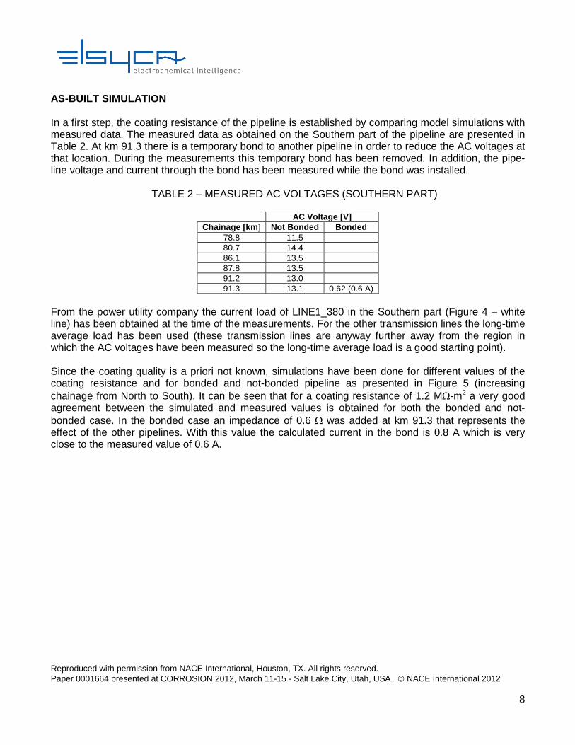
AS-BUILT SIMULATION In a first step, the coating resistance of the pipeline is established by comparing model simulations with measured data. The measured data as obtained on the Southern part of the pipeline are presented in Table 2. At km 91.3 there is a temporary bond to another pipeline in order to reduce the AC voltages at that location. During the measurements this temporary bond has been removed. In addition, the pipe-line voltage and current through the bond has been measured while the bond was installed.

TABLE 2 – MEASURED AC VOLTAGES (SOUTHERN PART)

AC Voltage [V] Chainage [km] Not Bonded Bonded

78.8 11.5 80.7 14.4 86.1 13.5 87.8 13.5 91.2 13.0 91.3 13.1 0.62 (0.6 A)

From the power utility company the current load of LINE1_380 in the Southern part (Figure 4 – white line) has been obtained at the time of the measurements. For the other transmission lines the long-time average load has been used (these transmission lines are anyway further away from the region in which the AC voltages have been measured so the long-time average load is a good starting point).

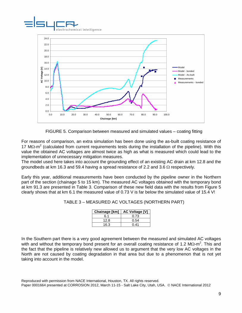
Since the coating quality is a priori not known, simulations have been done for different values of the coating resistance and for bonded and not-bonded pipeline as presented in Figure 5 (increasing chainage from North to South). It can be seen that for a coating resistance of 1.2 MΩ-m2 a very good agreement between the simulated and measured values is obtained for both the bonded and not-bonded case. In the bonded case an impedance of 0.6 Ω was added at km 91.3 that represents the effect of the other pipelines. With this value the calculated current in the bond is 0.8 A which is very close to the measured value of 0.6 A.


9

0.0

2.0

4.0

6.0

8.0

10.0

12.0

14.0

16.0

18.0

20.0

22.0

24.0

0.0 10.0 20.0 30.0 40.0 50.0 60.0 70.0 80.0 90.0 100.0

Chainage [km]

AC

Vol

tage

[V] Model

Model - bonded

Model - As-built

Measurements

Measurements - bonded

FIGURE 5. Comparison between measured and simulated values – coating fitting For reasons of comparison, an extra simulation has been done using the as-built coating resistance of 17 MΩ-m2 (calculated from current requirements tests during the installation of the pipeline). With this value the obtained AC voltages are almost twice as high as what is measured which could lead to the implementation of unnecessary mitigation measures. The model used here takes into account the grounding effect of an existing AC drain at km 12.8 and the groundbeds at km 16.3 and 59.4 having a spread resistance of 2.2 and 3.6 Ω respectively. Early this year, additional measurements have been conducted by the pipeline owner in the Northern part of the section (chainage 5 to 15 km). The measured AC voltages obtained with the temporary bond at km 91.3 are presented in Table 3. Comparison of these new field data with the results from Figure 5 clearly shows that at km 6.1 the measured value of 0.73 V is far below the simulated value of 15.4 V!

TABLE 3 – MEASURED AC VOLTAGES (NORTHERN PART)

Chainage [km] AC Voltage [V]

6.1 0.73 12.8 0.54 16.3 0.41

In the Southern part there is a very good agreement between the measured and simulated AC voltages with and without the temporary bond present for an overall coating resistance of 1.2 MΩ-m2. This and the fact that the pipeline is relatively new allowed us to argument that the very low AC voltages in the North are not caused by coating degradation in that area but due to a phenomenon that is not yet taking into account in the model.


10

However, additional investigation of the asset database of the pipeline owner did not result in any additional AC drainage or external bond that could explain the very low AC voltage at km 6.1. By using the model the influence of an additional AC drainage (with a resistance of 0.2 Ω) respectively at km 4.0 and 6.1 has been studied. Based on these extra model simulations - that result in a good agreement between the calculated and measured AC voltages in the North – additional field investigation has been done in the region between km 4.0 and km 6.1. This field survey indeed confirmed the simulation findings by exposing an additional current drainage that at present had not been added to the database of the pipeline owner (Figure 6). The drainage is located at km 4.8 somewhere in the middle of the region identified as the search area for anomalies!

FIGURE 6. AC current drainage exposed based on model simulations

Figure 7 presents a summary of the additional model simulations that lead to the exposure of the missing AC current drainage and the effect of adding that drainage to the model.


11

0.0

2.0

4.0

6.0

8.0

10.0

12.0

14.0

16.0

18.0

20.0

0.0 10.0 20.0 30.0 40.0 50.0 60.0 70.0 80.0 90.0 100.0

Chainage [km]

AC

Vol

tage

[V] Model - Bonded

Measurements - bonded

Extra Drainage km 4.0

Extra Drainage km 6.1

Existing Drainage km 4.8

FIGURE 7. Comparison between measured and simulated values (updated)

STUDY OF DIFFERENT SCENARIOS The above outlined methodology in which the pipeline coating quality is determined based on existing field data and the model further refined by performing dedicated simulations combined with additional measurements and field surveys allows to build a realistic model that is the starting point for further mitigation designs. This design needs to take into account the different conditions in which the power lines can operate (both in steady-state and fault conditions). For that reason the induced AC voltages on the pipeline need to be calculated for different scenarios:

• Steady-state o average load for all power lines (scenario 1) o full load for all power lines (scenario 2) o maintenance per circuit – other circuit carries full load current (scenarios 3-10)

• Single phase Fault o each individual line is faulted – results presented per circuit (scenarios 11-19)

Simulations have been done with the temporary bond at km 91.3 removed. In a first step all scenarios are calculated starting from the fitted model developed so far and the induced AC voltages are compared to the maximum allowed limit as set by the standards. In a second step, the results are evaluated and the mitigation calculations performed based on the worst-case scenarios. Finally, all scenarios are re-run with the mitigation in place and again checked versus the standards.


12

The steady-state and fault current information provided by the power utility company is presented in Tables 4 and 5.

TABLE 4 – STEADY-STATE (AVERAGE, FULL LOAD) CURRENTS

Power Line Station 1 Station 2 V [kV] # Circuits Full Load [A] Average Load [A] LINE1_380 Z M 380 2 4000 1200 (30%) LINE2_380 E M 380 2 4000 1200 (30%) LINE3_220 W M 220 2 2300 690 (30%) LINE4_110 V G 110 1 540 270 (50%) LINE5_110 V M 110 2 580 290 (50%)

TABLE 5 – FAULT CURRENTS

Power Line Station 1 Station 2 I1 [kA] I2->1 [kA] I2 [kA] I1->2 [kA] Duration [ms] LINE1_380 Z M 46.8 5.4 47.5 3.3 100 LINE2_380 E M 56.2 0.0 47.0 10.8 100 LINE3_220 W M 35.8 4.6 29.1 7.3 100 LINE4_110 V G 14.0 2.8 10.2 2.5 100 LINE5_110 V M 14.0 5.2 18.9 1.4 100

The results of the 19 scenarios are summarized in Table 6 and compared with the maximum allowed AC voltage which is 25 V for steady-state interference and 1500 V for faults with a duration of maximum 100 ms (national standard). From the results in Table 6 the following conclusions can be drawn:

• All of the steady-state scenarios exceed the maximum allowable limit of 25 A, with the full load scenario (all lines) giving the highest induced AC voltage

• single phasefaults in power line LINE1_380 exceed the maximum allowable limit of 1500 A • single phasefaults in all other power lines do not exceed the maximum allowable limit of 1500 A


13

TABLE 6 – RESULTS (DIFFERENT SCENARIOS – NOT MITIGATED)

Scenario Power Line Load Vac,allowed

[V] Vac,max

[V] Allowed ? [Yes/No]

1 All Average 25 28.9 No 2 All Full 25 96.4 No 3 LINE1_380 Maintenance (I-Full circuit 1) 25 62.5 No 4 LINE1_380 Maintenance (I-Full circuit 2) 25 80.7 No 5 LINE2_380 Maintenance (I-Full circuit 1) 25 40.5 No 6 LINE2_380 Maintenance (I-Full circuit 2) 25 44.1 No 7 LINE3_220 Maintenance (I-Full circuit 1) 25 28.9 No 8 LINE3_220 Maintenance (I-Full circuit 2) 25 28.9 No 9 LINE5_110 Maintenance (I-Full circuit 1) 25 28.9 No

10 LINE5_110 Maintenance (I-Full circuit 2) 25 28.9 No

11 LINE1_380 single phase fault (circuit 1) 1500 1907 No 12 LINE1_380 single phase fault (circuit 2) 1500 2218 No 13 LINE2_380 single phase fault (circuit 1) 1500 188 Yes 14 LINE2_380 single phase fault (circuit 2) 1500 187 Yes 15 LINE3_220 single phase fault (circuit 1) 1500 1110 Yes 16 LINE3_220 single phase fault (circuit 2) 1500 1134 Yes 17 LINE4_110 single phase fault (circuit 1) 1500 1485 Yes 18 LINE5_110 single phase fault (circuit 1) 1500 1433 Yes 19 LINE5_110 single phase fault (circuit 2) 1500 1158 Yes

The initial mitigation design therefore focuses on the full load scenario and a single phase fault in circuit 2 of power line LINE1_380. Figure 8 plots the pipeline AC voltages for the full load scenario (left Y-axis) and a single phase fault at tower M71 of LINE1_380 (right Y-axis), together with the allowed limit for both cases.

0.0

10.0

20.0

30.0

40.0

50.0

60.0

70.0

80.0

90.0

100.0

110.0

0.0 10.0 20.0 30.0 40.0 50.0 60.0 70.0 80.0 90.0 100.0

Chainage [km]

AC

Vol

tage

Ste

ady-

Sta

te [V

]

0.0

200.0

400.0

600.0

800.0

1000.0

1200.0

1400.0

1600.0

1800.0

2000.0

2200.0

2400.0

AC

Vol

tage

1-f

Fau

lt [V

]

Full Load

Steady-State Limit

1-f Fault LINE1_380 M71

1-f Fault Limit

FIGURE 8. Pipeline AC voltages for full load and single phase fault at M71 of LINE1_380


14

Power line LINE1_380 has 42 towers (numbered from M40 to M71). Tower M40 and M71 are at 17% and 30% of the developed length between both stations. Figure 9 presents the pipeline AC voltage for a single phase fault at LINE1_380 (middle line circuit 2) for different faulted towers (all towers have been faulted – only each of five has been presented to limit the amount of data in the graph).

0.0

200.0

400.0

600.0

800.0

1000.0

1200.0

1400.0

1600.0

1800.0

2000.0

2200.0

2400.0

0.0 10.0 20.0 30.0 40.0 50.0 60.0 70.0 80.0 90.0 100.0

Chainage [km]

AC

Vol

tage

[V]

M40

M45

M50

M55

M60

M65

M70

M71

1-f Fault Limit

FIGURE 9. Pipeline AC voltages for single phase fault at LINE1_380 (middle line circuit 2)

By using the simulation software it is relatively straightforward to design a mitigation strategy taking into account the following observations:

• the highest induced AC voltages in steady-state appear at both extreme ends of the pipeline (towers M40 and M71)

• the highest induced AC voltages in fault conditions appear near the routing of LINE1_380 Since power line LINE1_380 is near the Southern part of the pipeline, an AC drainage has been put in the North (at the begin of the pipeline) to start with (to mitigate the voltages at that end) while other drains have been added at strategic points in the region of LINE1_380. This resulted in a total of 4 AC current drainages each having a resistance of 1 Ω. Figure 10 shows a software screenshot of the AC drainages near LINE1_380.


15

FIGURE 10. AC current drainages added in the region of LINE1_380

Figure 11 plots the pipeline AC voltages for full load scenario (left Y-axis) and a single phase fault at tower M71 of LINE1_380 (right Y-axis) after mitigation.

0.0

2.0

4.0

6.0

8.0

10.0

12.0

14.0

16.0

18.0

20.0

22.0

24.0

26.0

0.0 10.0 20.0 30.0 40.0 50.0 60.0 70.0 80.0 90.0 100.0

Chainage [km]

AC

Vol

tage

Ste

ady-

Sta

te [V

]

0.0

200.0

400.0

600.0

800.0

1000.0

1200.0

1400.0

1600.0

AC

Vol

tage

1-f

Fau

lt [V

]

Full Load

Steady-State Limit

1-f Fault LINE1_380 M71

1-f Fault Limit

FIGURE 11. Pipeline AC voltages - full load and single phase fault at M71 of LINE1_380 (mitigated)

It can be seen that along the entire pipeline the AC voltages have been reduced to acceptable values. With the mitigation system in place, all other scenarios have been re-run and summarized in Table 7. It can be seen that for none of the scenarios the maximum induced voltage on the pipeline exceeds the allowable limit (either 25 or 1500 V).


16

TABLE 7– RESULTS (DIFFERENT SCENARIOS – MITIGATED)

Scenario Power Line Load Vac,allowed [V]

Vac,max [V]

Allowed? [Yes/No]

1 All Average 25 6.6 Yes 2 All Full 25 21.9 Yes 3 LINE1_380 Maintenance (I-Full circuit 1) 25 14.5 Yes 4 LINE1_380 Maintenance (I-Full circuit 2) 25 18.8 Yes 5 LINE2_380 Maintenance (I-Full circuit 1) 25 14.7 Yes 6 LINE2_380 Maintenance (I-Full circuit 2) 25 16.1 Yes 7 LINE3_220 Maintenance (I-Full circuit 1) 25 6.6 Yes 8 LINE3_220 Maintenance (I-Full circuit 2) 25 6.6 Yes 9 LINE5_110 Maintenance (I-Full circuit 1) 25 6.6 Yes

10 LINE5_110 Maintenance (I-Full circuit 2) 25 6.6 Yes

11 LINE1_380 single phase fault (circuit 1) 1500 617 Yes 12 LINE1_380 single phase fault (circuit 2) 1500 604 Yes 13 LINE2_380 single phase fault (circuit 1) 1500 69 Yes 14 LINE2_380 single phase fault (circuit 2) 1500 68 Yes 15 LINE3_220 single phase fault (circuit 1) 1500 527 Yes 16 LINE3_220 single phase fault (circuit 2) 1500 503 Yes 17 LINE4_110 single phase fault (circuit 1) 1500 1481 Yes 18 LINE5_110 single phase fault (circuit 1) 1500 1431 Yes 19 LINE5_110 single phase fault (circuit 2) 1500 1154 Yes

Note that with the mitigation system in place the largest AC voltage on the pipeline for a fault in power line LINE1_380 occurs when tower M46 is faulted as can be seen from Figure 12 (when looking at the same faulted line from circuit 2). Tower M46 is somewhere in the middle of two AC current drainages as can be seen from Figure 10. This again is a prove of the fact that when designing mitigation for AC induced voltages, one needs to consider all phenomena involved and take nothing for granted!

0.0

50.0

100.0

150.0

200.0

250.0

300.0

350.0

400.0

450.0

500.0

550.0

600.0

650.0

0.0 10.0 20.0 30.0 40.0 50.0 60.0 70.0 80.0 90.0 100.0

Chainage [km]

AC

Vol

tage

[V]

M40

M45

M46

M50

M55

M60

M65

M70

FIGURE 12. Pipeline AC voltages for single phase fault at LINE1_380 (mitigated)


17

CONCLUSIONS

In this paper, a simulation software suite has been presented that is able to model both resistive (“close field”) as inductive (“far field”) interference in ROW’s with pipeline and power transmission networks of any complexity. The software has been linked to the asset database of the pipeline owner and has been extended with an automated fault current module that faults each individual tower of all power lines which allows taking into account all possible scenarios in the mitigation design. It has been demonstrated how field data are used to update the model with realistic coating values and how the model was used to find anomalies in the input data. Secondly, the effect of different operating scenarios has been studied in order to predict mitigation for safe operation conditions. Based on the mitigation as designed by the software the induced AC voltages along the entire pipeline stayed below the allowable limit (either 25 or 1500 V) for all possible scenarios.

REFERENCES 1 “Cathodic Protection Level 1 Training Manual”, NACE International, 2000. 2 “Cathodic Protection Level 2 Training Manual”, NACE International, 2000. 3 NACE Standard Recommended Practice RP0177-2000, “Mitigation of Alternating Current and

Lightning Effects on Metallic Structures and Corrosion Control Systems”, 2000. 4 “AC Predictive and Mitigation Techniques – Final Report”, for Corrosion Supervisory Committee

PRC International, 1999. 5 “TL WorkstationTM Code: Version 2.3, Volume 3: CORRIDOR Manual”, EPRI Project 1902-07,

BIRL Final Report, EPRI, Palo Alto CA, June 1992. 6 F. Dawalibi, et al, “Power Line Fault Current Coupling to Nearby Natural Gas Pipelines, Volume 2:

User’s Guide for ECCAPP Computer Program, Final Report, EPRI Project RP 742-4, A.G.A. Project PR 176-510, Safe Engineering Services & Technologies Ltd, Montreal, Quebec, Canada, October, 1987.

7 L. Bortels, P. J. Stehouwer, K. Dijkstra, “Towards A Fully Integrated Pipeline Integrity Management Software”, NACE Corrosion Conference 2010, Paper No. 11131.

8 L. Bortels, J. Deconinck, C. Munteanu, V. Topa, “A General Applicable Model for AC Predictive and Mitigation Techniques for Pipeline Networks Influenced by HV Power Lines”, IEEE transactions on power delivery, vol. 21, no1, pp. 210-217, 2006.

9 L. Bortels, C. Munteanu, V. Topa, J. Deconinck, “A User-friendly Simulation Software for AC Predictive and Mitigation Techniques”, NACE Corrosion Conference 2008.

10 L. Bortels, J. Parlongue, W. Fieltsch, S. Segall, “Manage Pipeline Integrity by Predicting And Mitigating HVAC Interference”, NACE Corrosion Conference 2010, Paper No. 10114.

nace2012-0001664-accurate modelling and...

Documents