Na, J., Herrmann, G., & Zhang, K. (2017). Improving transientperformance of adaptive control via a modified reference model andnovel adaptation. International Journal of Robust and NonlinearControl, 27(8), 1351–1372. https://doi.org/10.1002/rnc.3636

Peer reviewed versionLicense (if available):CC BY-NCLink to published version (if available):10.1002/rnc.3636

Link to publication record in Explore Bristol ResearchPDF-document

This is the author accepted manuscript (AAM). The final published version (version of record) is available onlinevia Wiley at http://onlinelibrary.wiley.com/doi/10.1002/rnc.3636/abstract. Please refer to any applicable terms ofuse of the publisher.

University of Bristol - Explore Bristol ResearchGeneral rights

This document is made available in accordance with publisher policies. Please cite only thepublished version using the reference above. Full terms of use are available:http://www.bristol.ac.uk/red/research-policy/pure/user-guides/ebr-terms/

1

INTERNATIONAL JOURNAL OF ROBUST AND NONLINEAR CONTROL Int. J. Robust Nonlinear Control 2016; 00:1-21 Published online XX XXX 2016 in Wiley Online Library (wileyonlinelibrary.com). DOI: XXXXXXX

Improving Transient Performance of Adaptive Control via a Modified Reference Model and Novel Adaptation

Jing Na1,2 ∗, Guido Herrmann1 and Kaiqiang Zhang1 1 Department of Mechanical Engineering, University of Bristol, Bristol, BS8 1TR, UK

2 Faculty of Mechanical & Electrical Engineering, Kunming University of Science & Technology, Kunming 650500,China

SUMMARY

This paper presents a new model reference adaptive control (MRAC) framework for a class of nonlinear systems to

address the improvement of transient performance. The main idea is to introduce a nonlinear compensator to reshape

the closed-loop system transient, and to suggest a new adaptive law with guaranteed convergence. The compensator

captures the unknown system dynamics, and modifies the given nominal reference model and the control action. This

modified controlled system can approach the response of the ideal reference model. The transient is easily tuned by a

new design parameter of this compensator. The nominal adaptive law is augmented by new leakage terms containing

the parameter estimation errors. This allows for fast, smooth and exponential convergence of both the tracking error

and parameter estimation, which again improves overall reference model following. We also show that the required

excitation condition for the estimation convergence is equivalent to the classical persistent excitation (PE) condition.

In this respect, this paper provides an intuitive and numerically feasible approach to online validate the PE condition.

The salient feature of the suggested methodology is that the rapid suppression of uncertainties in the controlled system

can be achieved without using a large, high-gain induced, learning rate in the adaptive laws. Extensive simulations are

given to show the effectiveness and the improved response of the proposed schemes.

Received XXX 2016; Revised XXX 2016; Accepted XXX.

KEY WORDS: adaptive control; transient performance; nonlinear system; parameter estimation; robustness

1. INTRODUCTION

For the past decades, adaptive control [1-5] has been well developed due to its online learning ability to update control

parameters and to handle model uncertainties. Historically, there have been two major adaptive control frameworks

[2]: model reference adaptive control (MRAC) and self-tuning adaptive control (STAC). However, in both

methodologies, the adaptive laws are designed to minimize either the tracking control error or the observer/predictor

error based on the gradient descent method [1]. Although elegant mathematical results have been developed to

guarantee the steady-state performance of adaptive control systems, it is noted that the potentially poor transient

performance severely limits the practical application of adaptive control schemes. As frequently encountered in

practice, a small tracking error and smooth tracking performance during the first few seconds of operation are essential

for maintaining system safety. However, unlike linear time-invariant plants, characterizing and quantifying the

∗ Correspondence to: Jing Na, Department of Mechanical Engineering, University of Bristol, Bristol, BS8 1TR, UK ∗ E-mail: najing25@ 163.com Contract/grant sponsor: Marie Curie Intra-European Fellowships Project AECE with grant No. FP7-PEOPLE-2013-IEF- 625531 and National Natural Science Foundation of China (NSFC) with grants No. 61573174 and 61203066.

2

transient response of adaptive control systems are not trivial due to the inherently nonlinear and time-varying

properties [1]. This point can mainly be understood from the fact that the parameter estimation convergence speed of

gradient based adaptive laws is a function of the observer error and/or control error, which creates strong couplings.

Following the studies in the stability analysis of adaptive control systems in the 80s and the robustness enhancement in

the 90s, several attempts have been made to analyze the transient performance of adaptive control [6-8].

It is known that high gain adaptation in adaptive control with fast learning can help to suppress the uncertainties in

the transient response [9]. In particular for MRAC, a high learning rate can be useful for reducing the mismatch

between the uncertain dynamical system and the ideal reference model. However, the limitations and drawbacks of

high gain adaptation have also been well recognized and documented, i.e. high learning rate can lead to control signals

with high-frequency content, excite high-frequency unmodeled dynamics and thus even trigger instability in the

presence of measurement noise [10]. In this respect, it is necessary to carefully make a trade-off between the stability,

robustness and the transient performance in high gain adaptive control designs. To eliminate the high frequency

oscillations that come from fast adaptation in the adaptive control system, the authors of [9] introduced a low-pass

filter in the control loop to reshape both the transient and steady-state performance. This methodology is known as

L1-adaptive control. However, the original control objective, i.e. exact tracking of the ideal reference model, has been

slightly changed in L1-adaptive control due to the adopted filter dynamics. Barrier Lyapunov Function (BLF) based

control methods have been effective in addressing constraints imposed on the system output or state variables. In [11],

a BLF was employed to design an adaptive control for nonlinear strict-feedback systems, which should fulfill the

imposed output constraints. This idea was further extended to address time-varying output constraints [12].

Subsequently, a novel BLF was incorporated into iterative learning control (ILC) control for output constrained

systems [13], fault tolerant control for MIMO systems with state constraint [14], and nonlinear switched systems [15].

Thus, BLF-methods have helped to enhance transient responses in [16]. Another notable method to quantitatively

analyze and prescribe the transient performance of adaptive control systems is the prescribed performance function

(PPF) [17], which can characterize the maximum overshoot, convergence rate and steady-state error. Several

improved PPFs were also suggested for strict feedback systems [18], servo systems [19] and interconnected systems

[20]. The central feature of PPF control is that both the transient and steady-state performances can be examined and

prescribed during controller design. However, the initial system conditions should be appropriately known to set the

PPF parameters, and asymptotic convergence of the tracking error to zero may not be achieved in order to avoid the

potential singularity issue [19].

Recently, a new MRAC architecture has been developed by introducing an observer-like feedback term in the

reference model [21-23], which was subsequently named as the closed-loop reference model (CRM) in [21]. The key

idea is to add an observer-like term containing the state error between the reference model and the controlled system in

the reference model. Then the associated feedback coefficient can change the eigenvalues of the closed-loop system to

shape the error convergence response. In [24], this idea of CRM was further extended for adaptive output control for

systems that satisfy an accessible matching condition with a separation-like principle. However, it was shown in [23]

that a trade-off between the fast transient dynamics and the error feedback gains should be made to remedy the

potential peaking phenomenon. This idea has been further improved in [25] by using the high-frequency content

between the uncertain system and the reference model to limit the frequency component involved in the system error

dynamics. In [26], a new modification scheme of the reference model was suggested, where the compensator is

constructed based on the tracking error dynamics. In this adaptive control, an extra low-pass filter was used to achieve

3

robustness against measurement noise, because the induced residual term in the closed-loop system contains the

high-pass filtered component of the derivative of the tracking error.

In addition to modifying the reference model that generates the desired behavior to be followed, another major

element in MRAC, the adaptive law is also essential in adaptive control systems, i.e. fast and precise estimation of

unknown parameters can help to improve the transient response [1-5]. However, this point has drawn little attention in

the synthesis of MRAC. Recently, a low frequency adaptive law [27] was proposed by using a modification term to

filter out the high-frequency content in the update law, so that fast adaptation can be obtained by using large, high-gain

induced, learning rates. An alternative adaptive law with an optimal modification was presented in [28], which is

designed based on the minimization of the L2 norm of the tracking error by solving an optimal equation. Beyond the

well-known robust adaptive laws (e.g. e-modification and σ-modification), a new Q-modification [29] has been

developed using the integral of the derived uncertainty on a ‘moving’ time interval as a new leakage term. A derivative

free (without integration) adaptive law [30] was studied for MRAC, which uses the information of delayed estimates

and of current system state variables and control errors, so that the rapid time-varying dynamics can be estimated.

Although better control performance can be obtained, these modifications use the time histories of system state

variables and control actions, and thus a large history stack is required to store these required system dynamics; this

may impose increased computational costs. Moreover, the convergence of estimated parameters to their true values

cannot be guaranteed.

Another critical issue in the adaptive parameter estimation is the verification of persistent excitation (PE) condition,

which needs to be fulfilled to guarantee the error convergence [1]. The online validation of the PE condition, however,

has been considered as a crucial yet non-trivial problem, in particular for nonlinear systems. To address this issue, the

algorithm of [31] needs to test online the invertibility of a matrix and to compute its inverse when it is appropriate.

Recently, a concurrent learning adaptive control [32] was proposed to relax the PE condition, where specifically

selected and recorded data over finite intervals is incorporated concurrently with instantaneous data for adaptation;

this scheme also requests a large history stack to store past system information. In our previous work [33-35], we have

suggested a novel ‘direct’ parameter estimation framework based on the parameter estimation error, and proposed

several adaptive laws to achieve exponential and finite-time error convergence. The salient feature of our methods

[33-35] is that the parameter estimation is obtained without using the state derivatives and past system information,

and is independent of observer/predictor design. The ideas have been further extended to some particular control

system designs [33, 36]. We have also proved that the classical PE condition is sufficient to guarantee the required

excitation condition (i.e. an introduced auxiliary matrix is positive definite). Although this result partially solved the

problem of verifying the PE condition, the inverse of the claim (i.e. the positive definiteness of the introduced auxiliary

matrix implies the standard PE condition) was not proved in [33-35], which deserves further investigation for the

purpose of online verification of the exact PE condition.

In this paper, we will address the transient performance improvement of model reference adaptive control systems.

After revisiting the standard MRAC, we point out the potential solutions that can reshape the system transient

response, where two of them will be considered in this paper. A new system modification scheme is first suggested,

where a compensation term is constructed based on the tracking error dynamics and appropriate filter operations. This

compensator is used in both the reference model and control action to adjust the reference model and to reshape the

closed-loop control system. This can be achieved because the introduced compensator can rapidly suppress the

undesired uncertainties in the controlled system in comparison to the ideal reference model. Consequently, high gain

4

learning in the adaptive laws is not necessary for eliminating the transient error dynamics. We show that the introduced

compensation term does not change the original steady-state characteristics and it makes the states of the controlled

system approach the response of the desired reference system faster and smoother in the transient time by

appropriately choosing a design parameter. Thus, the original control objective to follow a reference model can be

retained. We further consider the improvement on the transient performance by modifying the adaptive law to achieve

exponential convergence of both the tracking error and parameter estimation simultaneously. For this purpose, the

originally suggested adaptive laws in our work [33-35] have been further explored considering the error dynamics to

provide new leakage terms, which contain the parameter estimation error. In particular, we prove in this paper that the

standard PE condition is equivalent to an alternative excitation condition (i.e. positive definiteness of an auxiliary

matrix). Thus, this paper suggests an indirect but feasible and intuitive method to online verify the exact PE condition.

Simulation results are provided to validate the theoretical studies, and to demonstrate the improved estimation and

control performance.

The main contribution of this paper can be briefly summarized as: 1) we propose a new method to modify the

reference model in the MRAC framework, where a compensation term is included to capture and suppress the transient

uncertainties. This compensation term is derived considering the control error system, and thus is different to the CRM

method [21-23] as shown in Section 3.1; 2) we design an improved adaptive law using new leakage terms with the

estimation error; this adaptive law can guarantee the convergence of the estimated parameters to their true values, and

thus improve the transient control response; 3) we present an indirect method to online verify the PE condition by

calculating the minimum eigenvalue or condition number of an auxiliary matrix.

Notation: Throughout this paper, , n

, n n× denote the real numbers, real column vectors with dimension 1n× and real

matrices with n n× , respectively. max ( )λ ⋅ and min ( )λ ⋅ define the maximum and minimum eigenvalues of the

corresponding matrices. ( )tr ⋅ is the matrix trace, ( )T⋅ , 1( )−⋅ and ( )+⋅ are the transpose, inverse and the generalized

inverse of matrices. Moreover, 2 and

∞ denote the 2L and L∞ norms and

F is the matrix Frobenius norm

2 ( )TF

A tr A A= . det( ) is the matrix determinant. The operators s, { }sL and { }1sL− are the Laplace variable, the

Laplace transform and the inverse Laplace transform, respectively.

Definition 1 [1]: A vector or matrix function φ is persistently excited (PE) if there exist 0,T > 0ε > such that

( ) ( ) , 0t T T

td I tφ τ φ τ τ ε

+≥ ∀ ≥∫ .

2. PROBLEM FORMULATION AND PRELIMINARIES

2.1 PROBLEM STATEMENT Consider the following uncertain dynamic system as

( ) ( ) [ ( ) ( )]x t Ax t B f x u t= + + (1)

where 1[ , ]= ∈

T nnx x x is the system state, ∈mu is the control input; ×∈n nA , ×∈n mB are system matrices,

and the pair ( , )A B is controllable and det( ) 0TB B ≠ ; ( )∈mf x is an unknown linear/nonlinear function.

The purpose of the control design is to obtain an adaptive control to make the state x of system (1) track the state

rx of the following desired reference model

5

( ) ( ) ( )r r r rx t A x t B r t= + (2)

where nrx ∈ is the state of the reference model, mr∈ is a given bounded command, n n

rA ×∈ is a Hurwitz system

matrix and n mrB ×∈ is the input matrix.

Assumption 1: The nonlinear uncertainties in (1) can be represented in the following parameterized form

( ) ( )Tf x W xφ= (3)

where d mW ×∈ is an unknown weight matrix and 1( ) [ ( ), , ( )]T ddx x xφ φ φ= ∈ is a known function vector.

Without loss of generality, the unknown parameter W is assumed to be constant. However, this condition can be relaxed to more generic cases where the parameter W is time-varying, which will be discussed in Section 3.

Remark 1: Assumption 1 is quite standard because the studied system (1) with (3) can cover both linear and nonlinear systems. This condition has been widely recognized and used in the adaptive control community (e.g. [1-5]) and can be fulfilled in most practical systems. For specific nonlinear systems that do not fulfill Assumption 1, a function approximator (e.g. neural network and fuzzy system) can be used to create a similar formulation as (3), which will be explained in Section 3.

Assumption 2: The pair ( , )r rA B in system (2) is a stable pair, and the matching condition r xA A BK= + , r rB BK= holds for

m nxK ×∈ , m m

rK ×∈ with det( ) 0rK ≠ .

The reference system matrix n nrA ×∈ is Hurwitz, so that there exist positive definite matrices , n nP Q ×∈ fulfilling

the Lyapunov equation Tr rA P PA Q+ = − .

In the following developments, it should be noted that for many time-dependent parameters, we omit for reasons of brevity the argument (t) after initial definition.

2.2 TRADITIONAL MRAC AND PERFORMANCE ANALYSIS Before introducing our idea, we first revisit the classical MRAC and its performance analysis. This will serve as the basis for further studies and also help to show our motivations. In the standard MRAC framework, the following control is used to make the state x of system (1) track the state rx of the reference model (2)

a nu u u= + (4)

where nu is the nominal control and au is the adaptive control, which are given as

n x ru K x K r= + (5)

ˆ ( )Tau W xφ= − (6)

where xK and rK are the feedback gain and feedforward gain, respectively; W is the estimation of the unknown

matrix W , which is online updated by the adaptive law

ˆ ( ) TW x e PBφ= Γ (7)

where 0Γ > is the adaptive gain, and re x x= − denotes the tracking error. It is noted that there are several modified

robust adaptive laws based on (7), e.g. optimal modification [28], σ-modification and e-modification proposed in [1-5]. Thus, the adaptive law (7) has been widely used although their robust modifications do not permit asymptotic convergence. We suggest here a modification of (7), which guarantees faster and exponential convergence. This modification is easily compared to the standard adaptive scheme (7). By substituting (4)~(6) into system (1), the closed-loop control system can be given as

( )Tr rx A x B r BW xφ= + +

(8)

Moreover, the tracking error dynamics can be obtained from (2) and (8) as

6

( )Tr re x x A e BW xφ= − = +

(9)

where ˆW W W= − is defined as the estimation error. Although the following lemma and its proof can be found in almost any adaptive control book, we represent it for the

purpose of completeness and of further analysis of the transient performance:

Lemma 1 [1-5]: For system (1) with the adaptive control (4)~(7) and reference system (2), all signals in the closed-loop system are

bounded and the tracking error e converges to zero asymptotically.

Proof: The proof of Lemma 1 can be found in any adaptive control book. Thus, please refer to [1-5] for details.

The aforementioned Lemma 1 shows that the controlled system state x converges to the reference state rx in the

steady-state. However, during the transient time, x may be far away from rx due to significant initial errors (0)e and

(0)W , which may lead to poor transient performance (e.g. convergence rate, smoothness). To show this point, we

analyze the transient response of the classical MRAC system considering the norms of e and W . Thus, we recall that

the Lyapunov function 1( )T TV e Pe tr W W−= + Γ used to prove the stability and convergence of MRAC. Then as

shown [1-5], the derivative of V can be obtained along (7) and (9) as 0TV e Qe= − ≤ . This further implies

min 0 0( ) ( ) ( ) ( ) (0) ( ) (0)

t tTQ e e d V d V V t Vλ τ τ τ τ τ≤ − = − ≤∫ ∫ (10)

so that from the limit case t →∞ it follows 2min2

(0) / ( )e V Qλ≤ , i.e. 2e L∈ .

Moreover, we quantify the L∞ norm bound of the tracking error from (10) as 22 1

min min max max min( ) / ( ) (0) / ( ) [ ( ) (0) ( ) (0) ] / ( )F

e V t P V P P e W Pλ λ λ λ λ−

∞ ∞≤ ≤ ≤ + Γ . (11)

It is shown in (11) that the L∞ norm of e depends on two components: the initial tracking error (0)e , and the initial

estimation error (0)W . Moreover, it is shown that the effects of (0)W can be reduced by using a large gain Γ , i.e. a

high gain adaptive law can rapidly suppress the effects of the initial estimation error (0)W in the transient period.

However, a large, high-gain induced, learning rate also causes undesirable high-frequency oscillations in adaptive systems, which may excite unmodeled dynamics and trigger instability. To address this issue, we quantify the 2L norm

bound of W , which correlates to the bound on the amplitude of high frequency oscillations in the adaptive systems [23]. As pointed out in [23], reducing the 2L norm of this derivative can implicitly decrease the amplitude of the high

frequency oscillations. From (7), we know that 2 2 2 22 2 2

max max 20 0ˆ|| || ( ) ( )W d PB e d PB eτ λ φ τ λ φ

∞ ∞

∞ ∞≤ Γ = Γ∫ ∫ (12)

Using the bound on 2

e in (10), we have

2

22 2 22 2 1max min max max max min

ˆ ( ) (0) ( ) ( ) ( ) (0) ( ) (0) ( )F

W PB V Q PB P e W Qλ φ λ λ φ λ λ λ−∞ ∞ ∞

≤ ≤ Γ Γ + Γ

(13)

The 2L norm of W in (13) increases as long as the learning gain Γ increases because both terms 2(0)e∞

and 2

(0)F

W are subject to 2max ( )λ Γ . Thus, the only way to uniformly decrease the 2L norm bound of (13) (and thus high

frequency oscillations) is to decrease the adaptive gain Γ .

The analysis in (11) and (13) shows the well-known trade-off in the adaptive control design, i.e. the high frequency oscillations in the adaptive system can be reduced by choosing a small learning gain, while a small learning gain leads to sluggish tracking error convergence. This is reasonable because only one parameter (adaptive learning gain Γ ) cannot provide sufficient degree-of-freedom to fulfill such two conflicting control objectives simultaneously. This fact motivates our current study to reshape the transient response of MRAC by altering the reference model and proposing a new adaptive law.

7

3. MODIFIED CONTROL ARCHITECTURE

3.1 MOTIVATION Following the analysis in Section 2, we further explore potential ways to improve the transient performance of

MRAC. For this purpose, we recall the reference model (2), the controlled system (8) and the associated error (9), and

then find the following solutions to modify the error convergence of e and to shape the response of x :

1) Improve the convergence of the control error e by changing the transition matrix of (9) (e.g. eigenvalue of

rA ): It is shown in (9) that the error convergence speed depends heavily on the location of the eigenvalues of rA . This

implies that the convergence of e to zero can be improved if the eigenvalues of matrix rA are shifted. This idea has

led to recent work [21-23], where an extra error feedback term ( )rK x x− is introduced in the reference model (2),

such that the matrix rA in (9) can be replaced by r rA B K+ . Hence, the feedback gain K provides one more

degree-of-freedom to manage the above two conflicting control objectives. However, the induced peaking phenomenon [23] should be carefully managed by tuning the parameters K and Γ .

2) Suppress uncertainties ( )TW xφ in the controlled system (8) by altering the reference model (2) and control

(4): The ultimate objective of control design is to make the controlled system (8) follow the ideal reference model (2).

Thus, if the uncertainties ( )TBW xφ in (8) can be appropriately compensated, the transient response can be

significantly improved. This idea has been initially studied in [26] by using a command governor architecture. In this paper, this observation will be further explored by introducing a feasible modification of the reference model and control action, which is independent of high frequency error content. Note both the reference model and control action are modified in this method, which is thus clearly different to the idea presented in [21-23], where only the reference model is adjusted.

3) Improve the convergence of the estimation error W in (8) and (9) by using a new adaptive law: As shown in

(8) and (9), if adequately fast convergence of the estimation error W to zero can be achieved, the undesired dynamics

( )TW xφ can also be suppressed to retain better transient performance. However, this observation has not drawn

particular attention in most available MRAC designs. Thus, this point will be addressed in this paper by suggesting a novel adaptive law with new leakage terms.

Fig. 1 Diagram of the proposed adaptive control framework.

Following these observations, this paper will present a new MRAC framework, where a newly modified reference

model is investigated to suppress the uncertainty ( )TW xφ in the closed-loop system (8), and a new adaptive law is

8

suggested to achieve faster convergence of W , which all benefit the transient convergence of the control error e . A block diagram of the modified adaptive control architecture with the altered reference model and new adaptive law is shown in Fig.1.

3.2 MODIFICATION ON REFERENCE MODEL We first present the modification scheme for the reference model (2) and the control action to compensate for the

effect of undesired dynamics ( )TBW xφ in the closed-loop system (8). For this purpose, we define the filtered variables

fe , fε and fφ as

ˆ

f f

f f

Tf f f

ke e e

k

k kW

φ φ φ

ε ε φ

+ = + = + =

(14)

where 0k > is a constant filter parameter. Note that (14) can be easily implemented by applying a filter operation

1/( 1)ks + on the available variables e , φ and ˆ TfkW φ .

We further define an auxiliary term nΕ∈ as

fr f f

e eA e B

kε

−Ε = + − (15)

Then, the reference model in (2) and nominal control (5) can be modified by using a new command signal r as

dr r G= + Ε (16)

where 1 1( )T TrG K B B B− −= is a known matrix, dr is a given bounded command signal, and Ε is the signal used to

reshape the reference model and control via r in (16). Note that in Section 2, r denotes the external command for the reference model (2), while in this section and the remainder sections, dr is used to replace this external command.

In this case, we substitute the modified command (16) into the reference model (2), system (1) and control (4)~(5), and denote 1( )T TF B B B−= , then the modified reference model can be given as

r r r r dx A x B r BF= + + Ε (17)

and the controlled system can be given as

( )Tr r dx A x B r BF BW xφ= + + Ε +

(18)

It should be noted that the tracking error dynamics between (17) and (18) do not change (i.e. the tracking error equation (9) still holds for (17)~(18)), because the modified command r in (16) is used in both the reference model (2) and the nominal control (5). Thus, we have the following results:

Theorem 1: For system (1) with the reference model (17) including a modified command given in (14)~(16), adaptive control (4)~(7) is used, then all signals in the closed-loop control system are bounded and the tracking error e converges to zero asymptotically. Moreover, for any finite filter parameter 0k > in (14), lim 0

t→∞Ε = and lim dt

r r→∞

= hold.

Proof: From the modified reference model (17) and the controlled system (18), one can obtain that the closed-loop error dynamics of e are the same as shown in (9), and the adaptive law (7) is used. Thus, the two equations used for the stability analysis are the same as those used in the standard MRAC in Lemma 1, so that the proof of asymptotic

convergence for e to zero can be conducted by using the Lyapunov function 1( )T TV e Pe tr W W−= + Γ . This is similar

to that shown in Lemma 1, which we will not repeat again.

Moreover, when 0e → and 0fe → hold for t →∞ , we can verify from (7) that ˆ 0W → , which implies 0fε →

from (14). Consequently, lim 0t→∞

Ε = can be proved based on (15), and lim dtr r

→∞= is also true according to (16). ◇

Remark 2:

9

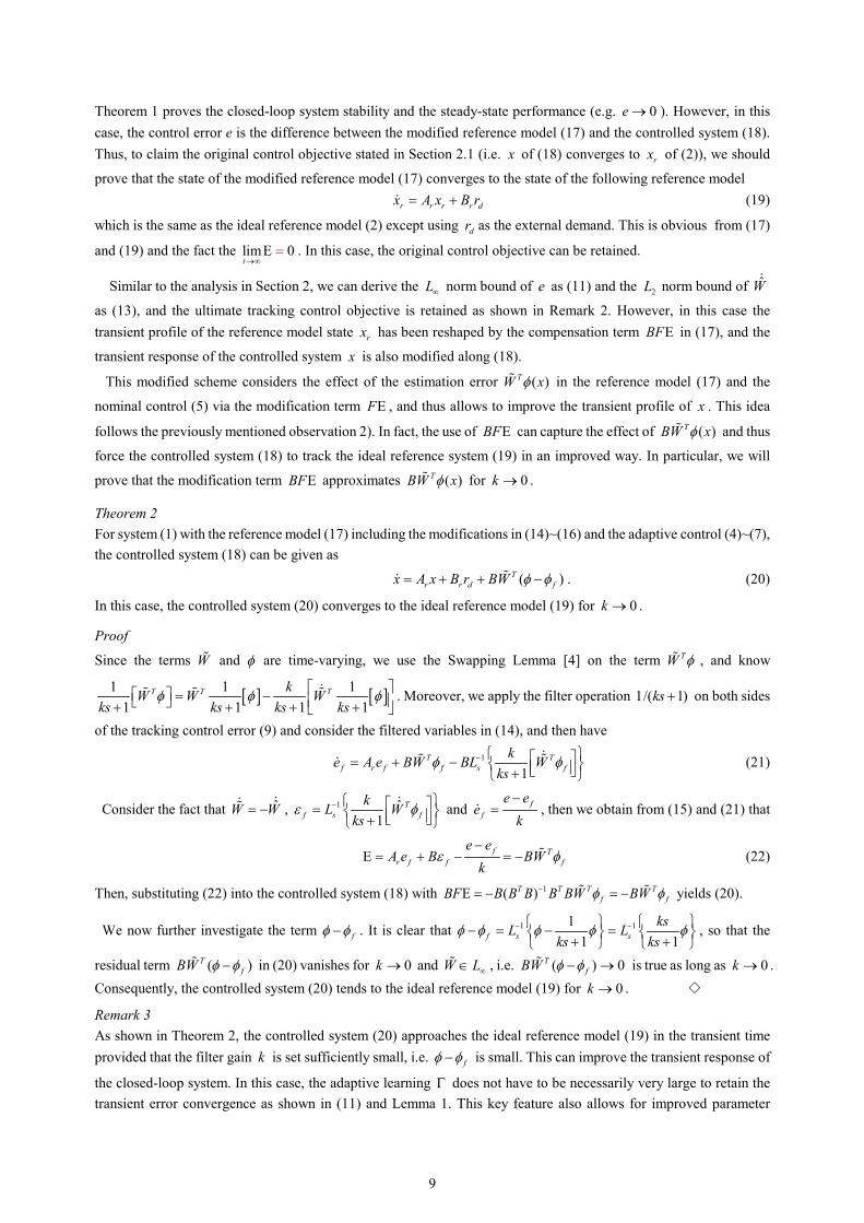
Theorem 1 proves the closed-loop system stability and the steady-state performance (e.g. 0e → ). However, in this case, the control error e is the difference between the modified reference model (17) and the controlled system (18). Thus, to claim the original control objective stated in Section 2.1 (i.e. x of (18) converges to rx of (2)), we should

prove that the state of the modified reference model (17) converges to the state of the following reference model

r r r r dx A x B r= + (19)

which is the same as the ideal reference model (2) except using dr as the external demand. This is obvious from (17)

and (19) and the fact the lim 0t→∞

Ε = . In this case, the original control objective can be retained.

Similar to the analysis in Section 2, we can derive the L∞ norm bound of e as (11) and the 2L norm bound of W

as (13), and the ultimate tracking control objective is retained as shown in Remark 2. However, in this case the transient profile of the reference model state rx has been reshaped by the compensation term BFΕ in (17), and the

transient response of the controlled system x is also modified along (18).

This modified scheme considers the effect of the estimation error ( )TW xφ in the reference model (17) and the

nominal control (5) via the modification term FΕ , and thus allows to improve the transient profile of x . This idea

follows the previously mentioned observation 2). In fact, the use of BFΕ can capture the effect of ( )TBW xφ and thus

force the controlled system (18) to track the ideal reference system (19) in an improved way. In particular, we will

prove that the modification term BFΕ approximates ( )TBW xφ for 0k → .

Theorem 2 For system (1) with the reference model (17) including the modifications in (14)~(16) and the adaptive control (4)~(7), the controlled system (18) can be given as

( )Tr r d fx A x B r BW φ φ= + + −

. (20)

In this case, the controlled system (20) converges to the ideal reference model (19) for 0k → .

Proof

Since the terms W and φ are time-varying, we use the Swapping Lemma [4] on the term TW φ , and know

[ ] [ ]1 1 11 1 1 1

T T TkW W Wks ks ks ks

φ φ φ = − + + + +

. Moreover, we apply the filter operation 1/( 1)ks + on both sides

of the tracking control error (9) and consider the filtered variables in (14), and then have

1

1T T

f r f f s fke A e BW BL W

ksφ φ− = + − +

(21)

Consider the fact that ˆW W= −

, 1 ˆ1

Tf s f

kL Wks

ε φ− = + and f

f

e ee

k−

= , then we obtain from (15) and (21) that

f Tr f f f

e eA e B BW

kε φ

−Ε = + − = − (22)

Then, substituting (22) into the controlled system (18) with 1( )T T T Tf fBF B B B B BW BWφ φ−Ε = − = − yields (20).

We now further investigate the term fφ φ− . It is clear that 1 111 1f s s

ksL Lks ks

φ φ φ φ φ− − − = − = + +

, so that the

residual term ( )TfBW φ φ− in (20) vanishes for 0k → and W L∞∈ , i.e. ( ) 0T

fBW φ φ− → is true as long as 0k → . Consequently, the controlled system (20) tends to the ideal reference model (19) for 0k → . ◇

Remark 3 As shown in Theorem 2, the controlled system (20) approaches the ideal reference model (19) in the transient time provided that the filter gain k is set sufficiently small, i.e. fφ φ− is small. This can improve the transient response of

the closed-loop system. In this case, the adaptive learning Γ does not have to be necessarily very large to retain the transient error convergence as shown in (11) and Lemma 1. This key feature also allows for improved parameter

10

estimation. As discussed in (13), the 2L norm bound of W correlates to the amplitude of high-frequency oscillations,

and can be diminished by using a small learning gain Γ .

The above claims can be further shown in an alternative way by comparing the responses of the original controlled system (8) (with the original reference model (2)) and the new controlled system (20) (with the modified reference model (17)) to the ideal reference model (19). For comparison, we derive the solution of (19), (8) and (20) as

( )

0( ) (0) ( )r r

tA t A tr r r dx t e x B e r dτ τ τ−= + ∫ (23)

( ) ( )

0 0( ) (0) ( ) ( ) ( )r r r

t tA t A t A t Tr dx t e x B e r d B e W dτ ττ τ τ φ τ τ− −= + +∫ ∫ (24)

( ) ( )

0 0( ) (0) ( ) ( ) ( ) ( )r r r

t tA t A t A t Tr d fx t e x B e r d B e W dτ ττ τ τ φ τ φ τ τ− − = + + − ∫ ∫ (25)

Denoting the difference between the ideal reference (19) and the controlled systems as re x x= − and assuming

(0) (0)rx x= (i.e. (0) 0e = ), we can apply the fact ( )min0

1/ ( )rt A t

re d Aτ τ λ− ≤∫ and have

For original MRAC: ( )

0( ) ( ) ( )r

t A t Te t B e W dτ τ φ τ τ−= ∫ (26)

max min( ) / ( )re B W Aλ φ λ∞ ∞∞≤ (27)

For modified MRAC: ( )

0( ) ( ) ( ) ( )r

t A t Tfe t B e W dτ τ φ τ φ τ τ− = − ∫ (28)

max min( ) / ( )f re B W Aλ φ φ λ∞ ∞∞≤ − (29)

Consider 1

1f sksL

ksφ φ φ− − =

+ and Theorem 2, we can set k sufficiently small. It is also true that

fφ φ φ∞∞

− ≤ holds [37] for any continuous regressor φ . Hence, the transient tracking performance is significantly

improved for the modified MRAC with a small filter coefficient k .

Moreover, as shown in (29), the transient bound of e depends on the bound of W ; this illustrates that the transient

response can also be further improved by accelerating the convergence of W . This fact motivates our further idea to modify the adaptive law (7) to be presented in the next subsection.

3.3 NEW ADAPTIVE LAW

In Section 3.2, the convergence of the estimation error W to zero with the gradient adaptive law (7) may be difficult because the online validation of the required PE condition is difficult. However, as pointed out in the above

observation 3) and shown in (29), fast convergence of W can also help to improve the transient response of e and x .

Thus, we will modify the adaptive law (7) in terms of new leakage terms to guarantee the convergence of W to zero. We define the auxiliary matrix d dM ×∈ and vector d mN ×∈ as

, (0) 0

ˆ , (0) 0

Tf f

T Tf

M M M

N N F MW N

γφ φ

γφ

= − + =

= − − Ε − =

(30)

where 0> and 0γ > are design parameters, and 1( )T TF B B B−= exists for any det( ) 0TB B ≠ .

Then we provide an alternative adaptive law as

1 2ˆ T T T

fW e PB N Fφ κ κ φ = Γ + − Ε (31)

where 0Γ > is the adaptation gain, 1 0κ > and 2 0κ > are positive constants, and Ε is the variable defined in (15).

Before we prove the convergence of the adaptive law (31), we will first study the relationship between the matrices M and N , which gives the following Lemma:

11

Lemma 2

For the variables defined in (30), then we have N MW= .

Proof From (30), we obtain the solution of ( )M t as

( )

0( ) ( ) ( )

t t Tf fM t e dτγ φ τ φ τ τ− −= ∫ (32)

Then consider the fact TfBW φΕ = − , it follows that

0

ˆ

( ) ( )

t t t T T tf

tt t T Tf f f f

e N e N e F e MW

e N e W e d Wτ

γ φ

γ φ φ γ φ τ φ τ τ

= − − Ε −

= − + + ∫

(33)

so that

0( ) ( )

tt t t T Tf f f fe N e N e W e d Wτγ φ φ γ φ τ φ τ τ+ = + ∫

. (34)

Then the equation (34) can be further rewritten as

0( ) ( ) ( ) ( )

tt Tf f

d de N t e d W tdt dt

τγ φ τ φ τ τ = ∫

(35)

Since the initial condition is set as (0) (0) 0M N= = , we apply the integral on both sides of (35) and obtain

0( ) ( )

tt Tf fe N e d Wτγ φ τ φ τ τ= ∫

(36)

which together with (32) implies

N MW= (37) This completes the proof. ◇

We now address the relationship between the positive definiteness of M and the standard PE condition. The following Lemma significantly improves the result of [33, 36], where only the first part has been provided.

Lemma 3 If the vector φ in (3) is PE, then for any 0> , the matrix M in (30) is positive definite, i.e. min ( ) 0Mλ σ> > . On the

other hand, the positive definiteness of M also implies that φ is PE.

Proof It is shown that the transfer function 1/( 1)ks + in (14) is stable, minimum phase and strictly proper [1], then the PE

condition of fφ is equivalent to the PE condition of φ because fφ is the filtered version of φ . Moreover, from

Definition 1, the PE condition ( ) ( )t T T

f ftd Iφ τ φ τ τ ε

+≥∫ equals to

-( ) ( )

t Tf ft T

d Iφ τ φ τ τ ε≥∫ for 0t T> > .

We first prove that if fφ is PE, then M is positive definite. Based on the above analysis, if fφ is PE, then

-( ) ( )

t Tf ft T

d Iφ τ φ τ τ ε≥∫ holds for 0t T> > . For the integration interval [ , ]t T tτ ∈ − , it follows that t Tτ− ≤ so that

( ) 0t Te eτ− − −≥ > is true, then we know ( ) ( ) ( ) ( ) ( )

t tt T T T Tf f f ft T t T

e d e d e Iτ φ τ φ τ τ φ τ φ τ τ ε− − − −

− −≥ ≥∫ ∫ (38)

Moreover, it can be verified for all 0t T> > that ( ) ( )

0( ) ( ) ( ) ( )

t tt T t Tf f f ft T

e d e dτ τφ τ φ τ τ φ τ φ τ τ− − − −

−>∫ ∫ (39)

From (38)~(39), one can conclude that ( )

0( ) ( ) ( ) ( )

t tt T T T Tf f f ft T

e d e d e IM τ φ τ φ τ τ φ τ φ τ τ ε− − − −

−= > ≥∫ ∫ (40)

This implies that M is positive definite and thus min ( ) 0Mλ σ> > is true for Teσ ε−= .

Finally, we will prove that if M is positive definite, then fφ is PE. If M is positive definite, i.e.

12

( )

0( ) ( )

t t Tf fM e d Iτ φ τ φ τ τ ε− −= ≥∫ holds, we have

( ) ( ) ( ) 2

0 0( ) ( ) ( ) ( ) ( ) ( ) || || ( ) ( )

Tt t T t tt T t T t T Tf f f f f f f f ft T t T

eI e d e d e d I dτ τ τε φ τ φ τ τ φ τ φ τ τ φ τ φ τ τ φ φ τ φ τ τ−−− − − − − −

∞− −≤ = + ≤ +∫ ∫ ∫ ∫

(41)

The last inequality is obtained by using the facts ( )

0/

t T t Te d eτ τ− − − −≤∫

and ( )0 1t Te− −< ≤ for [ , ]t T tτ ∈ − . Thus,

Eq.(41) implies †( ) ( ) , for

t Tf ft T

d I t Tφ τ φ τ τ ε−

≥ ≥∫ (42)

where † 2|| || / 0Tfeε ε φ−

∞= − >

for sufficiently large and T . This implies that fφ is PE, and thus φ is PE. ◇

Now, we summarize the main results of this paper as:

Theorem 3 Assume system (1) and the reference model (17) with the modifications in (14)~(16), the adaptive control (4)~(6) with the new adaptive law (31). If φ in (3) is PE, then all signals in the closed-loop control system are bounded, and the

tracking error e and estimation error W converge to zero exponentially. Moreover, for any finite filter parameter 0k > in (14), lim 0

t→∞Ε = and lim dt

r r→∞

= hold.

Proof

We have proved N MW= as in Lemma 2. Moreover, by considering the fact TfBW φΕ = − from (22), we obtain the

estimation error dynamics of (31) as

1 2ˆ T T

f fW W e PB MW Wφ κ κ φ φ= − = −Γ −Γ −Γ

(43)

We choose the same Lyapunov function as 1( )T TV e Pe tr W W−= + Γ , consider the fact Tf fφ φ is nonnegative

provided that φ in (3) is PE and min ( ) 0Mλ σ> > , and calculate the derivative of V along (9) and (43) as

1 2 12 ( ) 2 ( ) 2 ( )T T T T T Tf fV e Qe tr W MW tr W W e Qe tr W MW Vκ κ φ φ κ α= − − − ≤ − − ≤ − (44)

where { }1min max 1 maxmin ( ) / ( ), 2 / ( )Q Pα λ λ κ σ λ −= Γ is a positive constant. Then according to the Lyapunov theorem,

V and the errors e and W converge to zero exponentially with the rate α . This further implies that W , x and φ

are bounded and thus lim 0t→∞

Ε = holds based on (22), which in turn guarantees lim dtr r

→∞= from (16). Finally, one can

verify from (4)~(6) that u is bounded. Moreover, e is bounded and satisfies 0e → using (9), while ˆ 0W → based on (31). ◇

Remark 4 The suggested modification of the reference model and control can be extended to generic time-varying systems with

disturbances, noise and nonlinearities. In this case, function approximators (e.g. neural network and fuzzy system) can

be used, such that Assumption 1 can be relaxed to the following formulation

( , ) ( ) ( ) ( , )Tf x t W t x t xφ ω= + (45)

where ( ) d mW t ×∈ is an unknown time-varying matrix and ( , ) mt xω ∈ is an unknown residual error, which are

bounded by 1 2 3, ,W Wη η ω η≤ ≤ ≤ for positive constants 1 2 3, ,η η η . In this case, the control error (9) is

reformulated as ( )Tre A e BW x Bφ ω= + +

. The compensation term obtained from (15) is equivalent to

1

1T T

f f s fkBW B BL W

ksφ ω φ− Ε = − − + +

, which can capture the effects of the unknown disturbance ω (note fω

is the filtered version of ω , which is used only for analysis) and time-varying dynamics W . Ε can compensate for the dynamics of ω and W in the controlled system T

r r dx A x B r BF BW Bφ ω= + + Ε + +

. In this case, the Lyapunov

analysis in the proof of Theorem 3 is modified as 11 1 12 2 ( ) 2 ( )T T T TV e Qe e PB tr W MW tr W W Vω κ α β−= − + − + Γ ≤ − +

13

for positive constants 1α , 1β . Then we can show that the estimation error and the control error are all bounded. Moreover, the formulation (45) can also be used for systems [38] that cannot be linearly parameterized as (3) because the time-varying parameter ( )W t can be employed to model unknown nonlinearities [26].

Remark 5

The modified adaptive law (31) introduces new leakage terms T Tf Fφ Ε and N , which contain the estimation error W

(note that TfBW φΕ = − and N MW= ). These new leakage terms can lead to a quadratic term in W in the above

Lyapunov analysis, such that exponential convergence of both the tracking error e and estimation error W can be proved simultaneously. This newly suggested adaptive law can improve the transient performance of the controlled system (20), which can approach the ideal reference model (19) as we have explained in (29). This is clearly different to the claims in Theorem 1, where only asymptotic convergence of the tracking error e is proved.

Remark 6 A required condition for proving the parameter estimation convergence is that the regressor vector φ is PE. In the

modified adaptive law (31), the auxiliary matrix N contains the estimation error W associated with a nonnegative matrix M , which is the weighted integral of T

f fφ φ over the interval [0, t]. In this case, we have proved that the

standard PE condition can be represented as an alternative condition (i.e. positive definite property of matrix M ).

Remark 7 The online verification of the PE condition is regarded as nontrivial, in particular for nonlinear systems, and thus has remained an open problem. The importance of Lemma 3 lies in that it provides an intuitive and numerically feasible way to online test the PE condition. In Lemma 3, we show that the PE condition is equivalent to the positive definiteness of matrix M , which can be online verified by calculating the minimum eigenvalue of matrix M to test

for min ( ) 0Mλ σ> > . Moreover, it is interesting to note that 0

( ) ( ) ( )t T

f fM t dγ φ τ φ τ τ→ ∫ holds for sufficiently small

. Hence, the required condition tends to the so-called sufficient excitation (SE) condition 0

( ) ( )t T

f f d Iφ τ φ τ τ σ≥∫ ,

which is strictly weaker than the PE condition, i.e. it only requires PE to be satisfied for 0t = .

Remark 8 Compared to classical MRAC, the developed control shown in Fig.1 uses extra filter operations (14) and (30) to obtain the compensation term Ε and leakage term N , which can be easily implemented. In this framework, the filter coefficient k should be set as a small constant to maintain satisfactory tracking performance based on Theorem 2. On the other hand, k defines the bandwidth of the filter 1/( 1)ks + in (14). Consequently, k should be chosen as a

trade-off between robustness and control convergence. The forgetting factor in (30) can retain the boundedness of ,M N , and specify their convergence speed, but it introduces a d.c. gain of 1/ in (30); thus, cannot be too large.

The constant γ in (30) can help to maintain the amplitude of M , and thus increase the convergence speed of W . The

constants 1κ , 2κ affect the convergence of W ; however, 2κ cannot be set too large because the associated term T

f f Wφ φ in (43) with instant error information may be sensitive to noise. Finally, a notable feature of the control

proposed in this paper is that the transient error TW φ can be estimated and compensated via Ε as shown in (22).

Therefore, the gain Γ in the adaptive law (31) can be set small (or zero in the worst case as shown in the simulation), i.e. large, high gain-induced, learning rate that may trigger high-frequency oscillations is not necessary.

4. SIMULATION RESULTS

This section validates the suggested control using the following wing rock aircraft model [39, 40] as

1 1

2 2

0 1 0[ ( ) ]

0 0 1x x

f x ux x

= + +

(46)

14

where 1x is the roll angle and 2x is the roll rate, u denotes the aileron control input. The unknown aerodynamics are 3

1 1 2 2 3 1 2 4 2 2 5 1( ) | | | |f x x x x x x x xω ω ω ω ω= + + + + , which can be represented as the form of (3) with the unknown

parameter 1 2 3 4 5[ , , , , ]TW ω ω ω ω ω= and regressor 31 2 1 2 2 2 1( ) [ , ,| | ,| | , ]Tx x x x x x x xφ = . In this simulation, the unknown

parameters are 1 2 3 4 50.2314, 0.6918, 0.6254, 0.0095, 0.0214ω ω ω ω ω= = = − = = . The objective is to design an adaptive

control such that the roll dynamics of (46) can track the trajectory of an ideal reference model with a natural frequency 0.4ω = rad/s and a damping ratio 0.707ζ = . The external command dr is a square-wave with the period of 60 sec

and amplitude 20 rad. In this case, the nominal feedback control (5) can be obtained as [ 0.16, 0.57]xK = − − ,

0.16rK = . It is noted that this nominal control works well when ( ) 0f x = . However, it cannot guarantee the stability

of the aircraft (46) for ( ) 0f x ≠ because of the induced high frequency dynamics under operation conditions. Thus,

adaptive control (6) should be used with parameters as: 0.001k = , 0.3= , 0.5γ = , [ ]( )1,3,1,1,0.001diagΓ = ,

1 0.5κ = and 2 0.1κ = . The initial conditions are set as (0) [0,0,0,0,0]TW = and (0) [0.5,0]Tx = . These parameters

are designed based on the guidelines provided in Remark 8. Specifically, the filter coefficient k should be chosen as a trade-off between robustness and control convergence.

4.1 SIMULATION ANALYSIS OF MODEL REFERENCE CONTROL ELEMENTS

Then the following four cases are simulated: Case 1: Standard MRAC (4)~(7).

Case 2: Nominal control (4)~(5) with the modified reference model (14)~(17).

Case 3: Adaptive control (4)~(6) with new adaptive law (31).

Case 4: Adaptive control (4)~(6) with new adaptive law (31) and the modified reference model (14)~(17).

It is noted that the above case 2) is to simulate the worst case to validate the efficacy of the term GΕ , where the adaptive law (6) is switched off (i.e. 0Γ = ). Moreover, the case 3) is dedicated to show the advantage of the proposed adaptive law (31) with new leakage terms in comparison to the standard MRAC in Case 1).

Fig.2 depicts the performance of the standard MRAC (4)~(7). It is shown that the roll rate and control signals contain high-frequency oscillations (Fig.2(b~c)) although fair roll angle tracking response is achieved (Fig.2(a)). As

we analyzed following Lemma 1, a significant initial error (0)W could trigger high-frequency transient dynamics in

the adaptive systems. This is also because the used gradient adaptation (7) in this case study cannot achieve fast and precise estimation of unknown parameters (the estimated parameters are given in Fig.2(c), which do not converge to

their true values). Consequently, the effect of ( )TW xφ in the controlled system (8) cannot be eliminated effectively. In

particular, when the roll angle changes its sign, there are significant oscillations in the estimated parameters.

0 20 40 60 80 100 120

-10

-5

0

5

10

15x

r1x

1

t(s)

0 20 40 60 80 100 120

Syst

em S

tate

s

-4

-2

0

2

4

6

8

xr2

x2

0 20 40 60 80 100 120-4

-3

-2

-1

0

1

2

3

4

un

t(s)

0 20 40 60 80 100 120

Con

trol s

igna

ls

-50

0

50

ua

(a) Tracking profile of state variables. (b) Control signals.

15

W11

-2

0

2

W12

-2

0

2

W13

-4

0

2W

14

-2

0

4

t(s)

0 20 40 60 80 100 120

W15

-0.1

0

0.1

(c) Profile of the estimated parameters.

Fig.2 Simulation results of standard MRAC (4)~(7) (Case 1).

Thus, we are interested to test the capability of the modified reference model (14)~(17) with the compensator GΕ

to suppress the transient dynamics ( )TW xφ in the controlled system (8). To show the worst case, the adaptive law (6)

is turned off in the case 2) (i.e. the learning gain is set as 0Γ = , and ˆ ˆ( ) (0) 0W t W= = for all t >0 in the simulation,

and thus the adaptive control action 0au = ), and only the compensator GΕ is used to address compensation of the

nonlinearities ( )f x . In this case, the estimation error W W= leads to significant dynamics ( )TW xφ in the controlled

system (18), which should be compensated with Ε . Simulation results are given in Fig.3, from which we can find that a fast and satisfactory tracking response can be achieved, and the control signal is smooth. This implies that the induced compensator term GΕ can estimate the unknown dynamics ( )f x in the system, which is used to reshape the

nominal control nu . This result validates the claims in Theorem 1, i.e. the suggested filter operation (14) with only one

tuning parameter (i.e. filter constant 0k > ) can approximate the undesired transient error ( )TW xφ in the controlled

system (18). Since the adaptive control action au has not been used in this simulation, we can conclude that high-gain

adaptation or learning is not necessary, which also contributes to the smooth transient response.

0 20 40 60 80 100 120

-10

-5

0

5

10

15x

r1x

1

t(s)

0 20 40 60 80 100 120

Syst

em S

tate

s

-5

0

5

xr2

x2

0 20 40 60 80 100 120-40

-20

0

20

40

un

0 20 40 60 80 100 120

Con

trol s

igna

ls

-50

0

50

ua

t(s)

0 20 40 60 80 100 120

Com

pens

atio

n

-200

-100

0

100

200

(a) Tracking profile of state variables. (b) Control signals and compensator.

Fig.3 Simulation results of adaptive control (4)~(5) with modified reference model (14)~(17) (Case 2).

Moreover, the second idea to improve the transient response via the modified adaptive law is tested, where the

16

adaptive law (31) with new leakage terms 1 2, Tf fMW Wκ κ φ φ is used together with adaptive control (4)~(6). Fig.4

provides simulation results with the new adaptation, where superior performance over the standard MRAC is achieved. Specifically, the high frequency content in the adaptive laws can be diminished so that the state variables and control actions shown in Fig.4(a~b) are smoother than those in case 1) (Fig.2(a)~(b)). This result is expected because the newly included leakage terms can guarantee fast and precise parameter estimation as shown in Fig.4(c). Thus,

simultaneous tracking control and parameter estimation are achieved. However, the residual error TW φ during the

first 5sec, before W reaches zero, leads to a slightly oscillating transient response in the roll rate (Fig.4(a)). This could be further addressed by including the modified reference model (14)~(17).

0 20 40 60 80 100 120

-10

-5

0

5

10

15x

r1x

1

t(s)

0 20 40 60 80 100 120

Syst

em S

tate

s

-5

0

5

xr2

x2

0 20 40 60 80 100 120-4

-3

-2

-1

0

1

2

3

4

un

t(s)

0 20 40 60 80 100 120

Con

trol s

igna

ls

-30

-20

-10

0

10

20

30u

a

(a) Tracking profile of state variables. ` (b) Control signals.

W11

0

0.2

0.4

W12

0

0.5

1

W13

-0.6

-0.2

W14

-0.2

0

0.2

t(s)

0 20 40 60 80 100 120

W15

0

0.02

0

(c) Profile of estimated parameters.

Fig.4 Simulation results of adaptive control (4)~(6) with new adaptive law (31) (Case 3).

Finally, simulation results of adaptive control (4)~(6) with the new adaptive law (31) and the modified reference model (14)~(17) can be found in Fig.5, where the generated compensator GΕ is illustrated in Fig.5(b). It can be noted

that the transient error TW φ during the first 5 sec can be captured by the compensation term GΕ . Thus, the effects of TW φ can be suppressed using the modified reference model and the nominal control. Consequently, the transient

system response can be further improved (Fig.5(a)) in comparison to Fig.4(a). This result is explained in Theorem 3, i.e. the controlled system response of (18) behaves almost the same as the ideal reference model (19). It is found that the profiles of the estimated parameters are very similar to those shown in Fig.4(c).

17

0 20 40 60 80 100 120

-10

-5

0

5

10

15x

r1x

1

t(s)

0 20 40 60 80 100 120

Syst

em S

tate

s

-5

0

5

xr2

x2

0 20 40 60 80 100 120-4

-2

0

2

4

un

0 20 40 60 80 100 120

-20

0

20

Cont

rol s

igna

ls

ua

0 20 40 60 80 100 120-15

-10

-5

0

5

10

Com

pens

atio

n

t(s)

GE(t )

(a) Tracking profile of state variables. (b) Control signals and compensator.

Fig.5 Simulation results of adaptive control (4)~(6) with adaptive law (31) and modified reference model (14)~(17) (Case 4).

Fig. 6 illustrates the tracking control errors re x x= − of the above Case 1) ~ Case 4). One can find from Fig.6 that

the transient overshoots in both the roll angle and rate are significantly suppressed when the compensator GΕ is used (i.e. Case 2) and Case 4)), which means GΕ can capture and then compensate for the undesired transient dynamics. This in turn leads to smoother transient response and convergence to the steady-state although the use of filters for calculating the compensator GΕ may include phase lag in the roll angle responses. On the other hand, the newly introduced adaptive law (31) (Case 3)) can also eliminate the overshoots and maintain satisfactory steady-state performance in comparison to the standard MRAC (Case 1)).

0 5 10 15 20 25 30 35 40 45 50-1

-0.5

0

0.5

t(s)

0 5 10 15 20 25 30 35 40 45 50

-2

-1

0

1

2

3

4

0 2 4

-20

4

8

0 5 10-1

-0.5

0

0.5

30 35 40 45

0

0.2

0.4

Fig.6 Comparative tracking control errors of Case 1) ~Case 4).

4.2 COMPARATIVE ANALYSIS WITH PRESCRIBED PERFORMANCE CONTROL To further show the merit of this paper, we compare the proposed control with the prescribed performance function

(PPF) based control [19], which has also been proposed to address the transient performance of adaptive control

systems. For this purpose, we refer to [19] for the detailed control design procedure. Here, we provide the designed

PPF control for system (46) as

18

( )1

1 11 1 2 2 1 1

2 21

2 32 21

1 1ln , / , [ 1][ , ]2 1

ˆ ˆ ˆ ˆ ˆ ˆ, ,ˆ | |2 2

Tr

T Ta

e Sz S z r x x e s z z

k s s s su r r sr s

λ λ µ µµ λ λ

θ εφ φ θ φ φ σ θ ε σ εε ση η

−− + ∂

= = = = − − = Λ − ∂

= − − − = Γ − = Γ − +

(47)

where 0.5( ) (1 0.05) 0.05tt eµ −= − + is the prescribed performance function, 1 /eλ µ= is the normalized error of the

output tracking error 1 1 1re x x= − , 1 1 12 1 1

rµ λ λ = − + −

is a positive bounded time-varying coefficient. Other

simulation parameters are set as 0.5aΓ = Γ = , 1 2k = Λ = , 0.01η = and 1 2 3 0.1σ σ σ= = = .

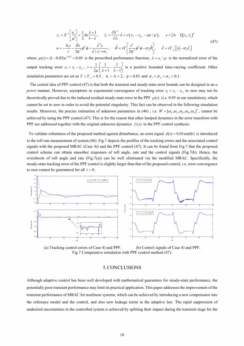
The central idea of PPF control (47) is that both the transient and steady-state error bounds can be designed in an a priori manner. However, asymptotic or exponential convergence of tracking error 1 1 1re x x= − to zero may not be

theoretically proved due to the induced residual steady-state error in the PPF ( )tµ (i.e. 0.05 in our simulation), which

cannot be set to zero in order to avoid the potential singularity. This fact can be observed in the following simulation results. Moreover, the precise estimation of unknown parameters in (46) , i.e. 1 2 3 4 5[ , , , , ]TW ω ω ω ω ω= , cannot be

achieved by using the PPF control (47). This is for the reason that other lumped dynamics in the error transform with PPF are addressed together with the original unknown dynamics ( )f x in the PPF control synthesis.

To validate robustness of the proposed method against disturbance, an extra signal ( ) 0.01sin(8 )d t t= is introduced

to the roll rate measurement of system (46). Fig.7 depicts the profiles of the tracking errors and the associated control signals with the proposed MRAC (Case 4)) and the PPF control (47). It can be found from Fig.7 that the proposed control scheme can obtain smoother responses of roll angle, rate and the control signals (Fig.7(b). Hence, the overshoots of roll angle and rate (Fig.7(a)) can be well eliminated via the modified MRAC. Specifically, the steady-state tracking error of the PPF control is slightly larger than that of the proposed control, i.e. error convergence to zero cannot be guaranteed for all 0t > .

0 20 40 60 80 100 120

Rol

l ang

le e

rror

-0.2

-0.1

0

0.1

0.2

0.3

0.4

0.5

t(s)

0 20 40 60 80 100 120

Rol

l rat

e er

ror

-0.8

-0.6

-0.4

-0.2

0

0.2

PPF MRAC

30 40 50 60-0.04

0

0.02

0 20 40 60 80 100 120

Con

trol s

igna

l -40

-20

0

20

40

t(s)

0 20 40 60 80 100 120-40

-20

0

20

40

(a) Tracking control errors of Case 4) and PPF. (b) Control signals of Case 4) and PPF.

Fig.7 Comparative simulation with PPF control method (47).

5. CONCLUSIONS

Although adaptive control has been well developed with mathematical guarantees for steady-state performance, the

potentially poor transient performance may limit its practical application. This paper addresses the improvement of the

transient performance of MRAC for nonlinear systems, which can be achieved by introducing a new compensator into

the reference model and the control, and also new leakage terms in the adaptive law. The rapid suppression of

undesired uncertainties in the controlled system is achieved by splitting their impact during the transient stage for the

19

reference model and the nominal control. In this case, a large, high-gain induced, learning rate that may trigger

high-frequency oscillations in the adaptation can be avoided; this in turn leads to smoother transient and convergence

to the steady-state. Consequently, we prove that the controlled system follows the ideal reference model, provided that

a sufficiently small filter parameter is used in the compensator. Moreover, we also suggest an improved robust

adaptive law by introducing new leakage terms to guarantee faster and precise estimation of unknown parameters; this

method can further reshape the transient response. In this respect, exponential convergence of both the tracking error

and estimation error can be proved simultaneously. Another contribution is that we provide a numerically feasible way

to online verify the classical PE condition, which is equivalent to the positive definiteness property of an auxiliary

matrix. Theoretical studies have been validated in terms of numerical simulations. The suggested ideas of modifying

the reference system and adaptive laws will be further explored for other adaptive architectures in our future work.

ACKNOWLEDGEMENTS

The work was supported by the Marie Curie Intra-European Fellowships Project AECE with grant No.

FP7-PEOPLE-2013-IEF-625531 and National Natural Science Foundation of China (NSFC) with grants No.

61573174 and 61203066).

REFERENCES

[1] Sastry S, Bodson M. Adaptive control: stability, convergence, and robustness. Prentice Hall: New Jersey, 1989. [2] Slotine JJE, Li W. Applied nonlinear control. Prentice Hall Englewood Cliffs, NJ, 1991. [3] Narendra KS, Annaswamy AM. Stable adaptive systems. Prentice-Hall, Inc. Upper Saddle River, NJ, USA, 1989. [4] Ioannou PA, Sun J. Robust Adaptive Control. Prentice Hall: New Jersey, 1996. [5] Krstic M, Kokotovic PV, Kanellakopoulos I. Nonlinear and adaptive control design. Wiley-Interscience New

York, 1995. [6] Krstic M, Kokotovic PV, Kanellakopoulos I. Transient-performance improvement with a new class of adaptive

controllers. Systems & Control Letters 1993; 21(6): 451-461. [7] Datta A, Ioannou PA. Performance analysis and improvement in model reference adaptive control. IEEE

Transactions on Automatic Control, 1994; 39(12): 2370-2387. [8] Zang Z, Bitmead RR. Transient bounds for adaptive control systems. IEEE Transactions on Automatic Control

1990; 39(1): 171-175. [9] Hovakimyan N, Cao C. L1 adaptive control theory: guaranteed robustness with fast adaptation. Siam:

Philedelphia, PA, 2010. [10] Rohrs CE, Valavani L, Athans M, Stein G. Robustness of continuous-time adaptive control algorithms in the

presence of unmodeled dynamics. IEEE Transactions on Automatic Control, 1985; 30(9): 881-889. [11] Tee KP, Ge SS, Tay EH. Barrier Lyapunov functions for the control of output-constrained nonlinear systems.

Automatica 2009; 45(4): 918-927. [12] Tee KP, Ren B, Ge SS. Control of nonlinear systems with time-varying output constraints. Automatica 2011;

47(11): 2511-2516. [13] Jin X, Xu J-X. Iterative learning control for output-constrained systems with both parametric and nonparametric

uncertainties. Automatica 2013; 49(8): 2508-2516. [14] Jin X. Adaptive fault tolerant control for a class of input and state constrained MIMO nonlinear systems.

International Journal of Robust and Nonlinear Control 2016; 26(2): 286-302. [15] Niu B, Zhao J. Barrier Lyapunov functions for the output tracking control of constrained nonlinear switched

systems. Systems & Control Letters 2013; 62(10): 963-971. [16] Jin X. Fault tolerant finite-time leader–follower formation control for autonomous surface vessels with LOS

range and angle constraints. Automatica 2016; 68: 228-236. [17] Bechlioulis CP, Rovithakis GA. Adaptive control with guaranteed transient and steady state tracking error

bounds for strict feedback systems. Automatica 2009; 45(2): 532-538. [18] Na J. Adaptive prescribed performance control of nonlinear systems with unknown dead zone. International

Journal of Adaptive Control and Signal Processing 2013; 27(5): 426-446.

20

[19] Na J, Chen Q, Ren X, Guo Y. Adaptive Prescribed Performance Motion Control of Servo Mechanisms with Friction Compensation. IEEE Transactions on Industrial Electronics 2014; 61(1): 486-494.

[20] Wang C, Lin Y. Decentralized adaptive tracking control for a class of interconnected nonlinear time-varying systems. Automatica 2015; 54: 16-24.

[21] Lavretsky E. Reference dynamics modification in adaptive controllers for improved transient performanceAIAA Guidance, Navigation, and Control Conference, : Portland, Oregon, 2011;1-13.

[22] Stepanyan V, Krishnakumar K. Adaptive control with reference model modification. Journal of Guidance, Control, and Dynamics 2012; 35(4): 1370-1374.

[23] Gibson TE, Annaswamy AM, Lavretsky E. On adaptive control with closed-loop reference models: transients, oscillations, and peaking. IEEE Access, 2013; 1: 703-717.

[24] Gibson TE, Zheng. Q, Annaswamy AM, Lavretsky E. Adaptive Output Feedback Based on Closed-Loop Reference Models. IEEE Tansactions on Automatic Control 2015; 60(10): 2728-2733.

[25] Yucelen T, De La Torre G, Johnson EN. Improving transient performance of adaptive control architectures using frequency-limited system error dynamics. International Journal of Control 2014; 87(11): 2383-2397.

[26] Yucelen T, Johnson E. A new command governor architecture for transient response shaping. International Journal of Adaptive Control and Signal Processing 2013; 27(12): 1065-1085.

[27] Yucelen T, Haddad WM. Low-frequency learning and fast adaptation in model reference adaptive control. IEEE Transactions on Automatic Control, 2013; 58(4): 1080-1085.

[28] Nguyen NT. Optimal control modification for robust adaptive control with large adaptive gain. Systems & Control Letters 2012; 61(4): 485-494.

[29] Volyanskyy KY, Haddad MM, Calise AJ. A new neuroadaptive control architecture for nonlinear uncertain dynamical systems: Beyond-and-modifications. IEEE Transactions on Neural Networks, 2009; 20(11): 1707-1723.

[30] Yucelen T, Calise AJ. Derivative-free model reference adaptive control. Journal of Guidance, Control, and Dynamics 2011; 34(4): 933-950.

[31] Adetola V, Guay M. Performance Improvement in Adaptive Control of Linearly Parameterized Nonlinear Systems. IEEE Transactions on Automatic Control 2010; 55(9): 2182-2186.

[32] Chowdhary G, Muhlegg M, Johnson E. Exponential parameter and tracking error convergence guarantees for adaptive controllers without persistency of excitation. International Journal of Control 2014; 87(8): 1583-1603.

[33] Na J, Herrmann G, Ren X, Mahyuddin MN, Barber P. Robust adaptive finite-time parameter estimation and control of nonlinear systems IEEE International Symposium on Intelligent Control (ISIC). IEEE: Denver, CO, USA, 2011;1014-1019.

[34] Na J, Mahyuddin MN, Herrmann G, Ren X. Robust adaptive finite-time parameter estimation for linearly parameterized nonlinear systems2013 32nd Chinese Control Conference (CCC). IEEE, 2013;1735-1741.

[35] Na J, Ren X, Xia Y. Adaptive parameter identification of linear SISO systems with unknown time-delay. Systems & Control Letters 2014; 66: 43-50.

[36] Na J, Mahyuddin MN, Herrmann G, Ren X, Barber P. Robust adaptive finite time parameter estimation and control for robotic systems. International Journal of Robust and Nonlinear Control 2015; 25(16): 3045-3071.

[37] Skogestad S, Postlethwaite I. Multivariable feedback control: analysis and design. Wiley New York, 2007. [38] Zhang Z, Xu S, Zhang B. Exact tracking control of nonlinear systems with time delays and dead-zone input.

Automatica 2015; 52: 272-276. [39] Singh SN, Yirn W, Wells WR. Direct adaptive and neural control of wing-rock motion of slender delta wings.

Journal of Guidance, Control, and Dynamics 1995; 18(1): 25-30. [40] Maity A, Höcht L, Holzapfel F. Higher-Order Direct Model Reference Adaptive Control with Generic Uniform

Ultimate Boundedness. International Journal of Control 2015; 88(10): 2126-2142.