N87-22719

IMPROVING STABILITY MARGINS

IN DISCRETE-TIME LQG CONTROLLERS

B. Tarik Oranc and Charles L. Ph1111ps

E1ectrical Engineering Department

Auburn University

Auburn, AL 36849

in

problems that may

assumptions; namely,

relative stability,

properties.

replace the

steady state,

compensator

Input, which

applications.

ABSTRACT

This paper discusses some of the problems encountered

the design of discrete-tlme stochastic controllers for

adequately be described by the "LQG"

the problems of obtaining

robustness, and disturbance

The paper proposes a dynamic compensator

optlmal full state feedback regulator gains

provided that all states are measurable.

increases the stablIIty marglns theat

in

has

may possibly be inadequate

Though the optimal regulator

acceptable

rejection

to

at

The

plant

practical

desirable

properties

a Kalman

stabI11ty

the observer based controller as Implemented with

filter, In a noisy environment, has Inadequate

margins. The proposed compensator ts designed to

match the return difference matrix at the plant input to that

of the optirr_l regulator while maintaining the optimality of

the state estimates as dictated by the measurement noise

characteristics.

417

https://ntrs.nasa.gov/search.jsp?R=19870013286 2018-05-21T02:59:22+00:00Z

418

I. INTRODUCTION

The design of robust stochastic

problems adequately described by the "LQG"

controllers for

assumptions has

been a

Doyle's

different approaches have been taken In order

various robust LQG controllers. It can be stated

that the approaches taken were to increase the

margins, namely the gain and phase margins at

fteld of active research tn

Ill and Doyle and Steln's [2]

recent years.

Introductory

to

Since

papers

design

generally

stability

the plant

Input, sufficiently so that the closed loop system remained

stable under large parameter changes In the plant and/or

sensor failures. It ts Important to note at this point that

most research has been on continuous time systems. The

robustness problem may be more pronounced in discrete time

controllers due to sampling rate limitations and the phase

lag associated with sampling.

In order to have a better understanding of the problem

it Is necessary to briefly review the respective parts of the

stochastic controller. The stochastic LQG controller ts

comprised of the LQ optimal feedback controller and the

Kalman filter based current ful] state observer. It has been

well established that the continuous time LQ controller based

system has excellent guaranteed stability margins, namely a

phase margin of at least 600 and an infinite gain margin.

Unfortunately the discrete time equivalent doesn't have these

guaranteed margins. However as the sampling period

approaches zero the stability margins approach those that of

the continuous time LQ contro]ler. The Kalman filter will

show

also be stable. However when the Kalman Filter Is used

estimate the state variables for feedback to the

controller the robustness properties of the system wllI

an excellent performance in estlmatlng states and will

to

LQ

not

be guaranteed. Doyle has given a simple example where a LQG

controller-filter combination has very small gain margins,

and hence Is not robust. An Investigation of the paper by

Johnson [3] exp]alns thls behavior of the LQG controllers.

Consider the state space representation of a plant For

which a LQG controller Is to be designed.

x(k+[) = Ax(R) + Bu(R) + Gw(k)

(t)y(k) = Cx(k) + v(k)

where

x(k)eR n , u(k)eR r , y(R)eR m

and w(k) and v(k) are uncorrelated, zero mean white gausslan

noise processes.

Denoting the constant Kalman Filter gains by KF and the

constant LQ gains by

equivalent of Theorem

O'Rellly [4].

Theorem :

that one

observer

K we considerc

8.3 as stated In

the discrete tlme

the monograph by

There exists a class of linear systems ( I

or more elgenvalues of (I - KFC)(A - BK c)

based feedback controller may lle outside

) such

of the

of the

unit circle In the complex plane though all elgenvalues of (A

- BK c) and all the elgenvalues of (A - KfCA) are designed to

lle with|n the unlt circle, and even though the system pairs

(A,B) , (A,C) are, respect|vely completely controllable and

completely observable.

419

The significance of this theorem lies tn the fact that

although the closed loop elgenvalues of the LQG system are

the union of the observer etgenvalues and optimal regulator

etgenvalues, and hence result in a stable closed loop system,

the eigenvalues of the controller may lie outside the unit

circle, therefore causing the controller to be unstable. It

may therefore be concluded that the LQG control system may

not be robust.

There have been three major approaches In alleviating

the robustness problem that may occur in LQG systems. In

light of the theorem all three methods will be investigated

In the same frame work. The first approach ts that of Doyle

and Stein [2]. They developed a robustness recovery

procedure in which they added fictitious process noise at the

plant Input. By controlling the way the fictitious noise

entered the plant Input they recovered the loop transfer

function (LTR) at the plant Input asymptotically as the noise

Intensity ts increased. This method has the drawback that

the system has to be square. A recent paper by Madlwale and

Williams [5] has extended the LTR procedure to minimum phase,

non-square and left-lnvertable systems with ful ! or reduced

order observer based LQG designs. It ts observed that the

LTR method actually results in the Kalman filter gains being

forced asymptotically Into a region where all etgenvalues of

the controller lte within the unit circle. The major problem

in this method Is that the Kalman filter Is no longer optimal

with respect to the true disturbances on the plant as its

elgenvalues have been shifted via the effective adjustment on

420

the process noise . Another disadvantage Is that

dB/decade roll-off associated wlth the LQG design Is

out Into the hlgh frequency range where unmodelled

frequency modes might be excited and cause Instability.

The second approach which was Initiated by Gupta

and by Moore et al [7] In separate papers was to

robustness In frequency bands where the problems

without changing the closed-loop characteristics

the 40

pushed

high

[6],

achieve

occurred

outstde

those frequency bands. Gupta used frequency-shaped cost

functtonals to achieve robustness by reducing filter gain

outside the model bandwidth. On the other hand Moore et al

[7] essentially Improvised on Doyle and Stein's LTR method by

adding fictitious colored noise Instead of white noise to the

process Input, thereby relocating both the KallT_n filter

etgenvalues and the controller elgenvalues. Recently

Anderson et al [B] have Investigated the relations between

frequency dependent control and state weighting In LQG

problems. Both of these procedures result in controller

etgenvalues that lie within the unit circle, thereby

overcoming the problems stated tn the theorem.

The last approach is due to Okada et al [9]. Their

approach Is drastically different from the previous

approaches. They have changed the structure of the LQG

controller by Introducing a feed-forward path from the

controller Input to the controller output. This Is

equivalent to Introducing an additional feedback loop from

the output to the Input of the plant. The crtterta for the

selection of the gains In this path Is to force the

421

control Ier

Ioop resu Its

propert Ies.

synthes Iz Ing

system [9].

to satisfy the circle criterion.

in a robust controller with

This additional

poor response

Therefore the response ts Improved by

an extended perfect model-following (EMPF)

This approach has the disadvantage that Its

statistical properties haven't been established.

it ts not always applicable theoretically.

practice it outperforms Doyle and Steln's LTR

some approximations as described In [9].

Furthermore

However, In

method with

The approach taken tn this paper ts an extension of the

LTR procedure. A dynamic compensator Is proposed to replace

the optimal feedback gains so as to recover the open loop

transfer function at the plant Input.

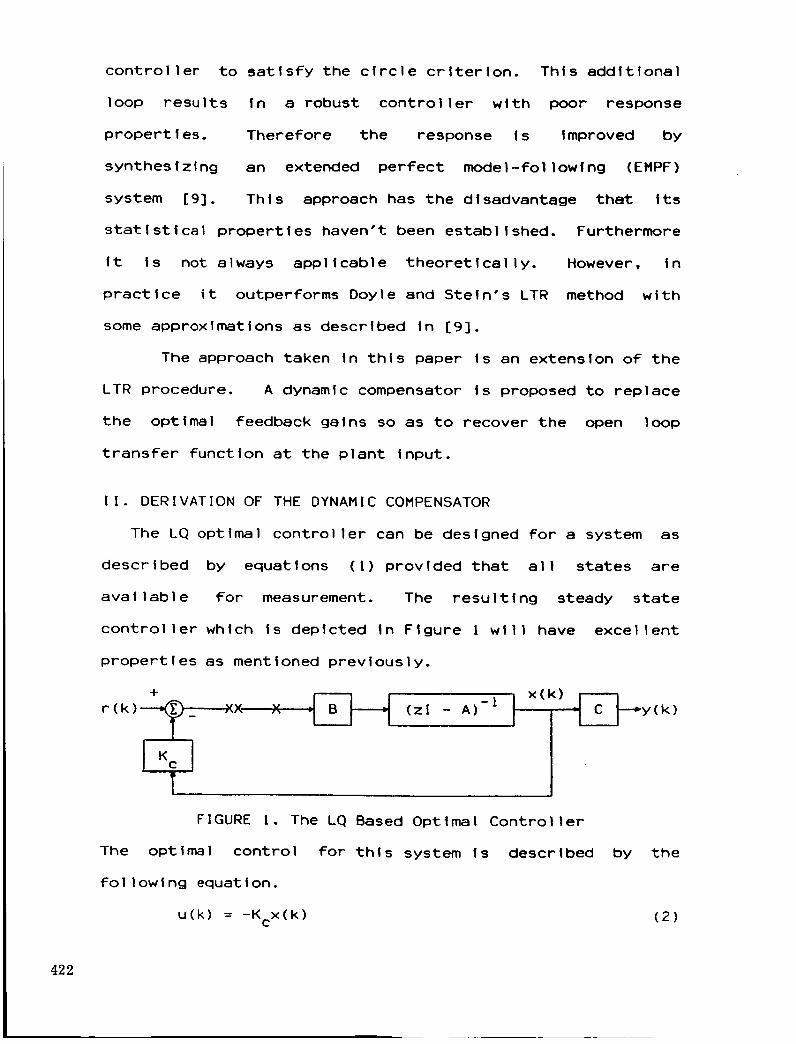
II. DERIVATION OF THE DYNAMIC COMPENSATOR

The LQ optimal controller can be designed for a system as

described by equations (I) provided that all states are

available for measurement. The resulting steady state

controller which ts depicted in Figure ! will have excellent

properties as mentioned previously.

+ D-"r(k)_X X = (zl - A) -1 ] x(k)

- I y(k)

FIGURE 1. The LQ Based Optimal Controller

The optimal control for this system Is described by the

following equation.

u(k) = -KcX(k) (2)

422

In the case that the state measurements are corrupted

by white gausslan noise an LQG controller can be designed In

which the Kalman filter ts used to estimate the states. The

LQG design results tn the following controller equations for

the Infinite horizon problem.

The Kalman filter Is described by

A

x(k+l) = Ax(k)+gu(k)+Kf[y(k+l)-CAx(k)-CBu(k)]

and the optimal control is described by

u(k) = -K x(k)c

Figure 2 depicts the LQG system.

(3)

(4)

+ x(k){_r(k)-_ (zI- A)-I I -,y(k)

F I z-,(,-Kfc)oII

x(k) I +z(zI - A) -1

I zcAIFIGURE 2. The LQG Based Optimal Controller/Observer

The following three properties of the system have been

established :

PI: The closed loop transfer function rl_trices from r(k) to

x(k) are Identical In both the LQG and LQ systems.

P2: The loop transfer function matrices with the loops broken

at XX are Identical in both implementations.

P3: The loop transfer function rl_trices with the loops broken

at X are generally different. Furthermore the LQG open-loop

system might possibly have unstable poles.

423

The return difference ratios of the LQG and LQ systems are

given by the following expressions.

Tiqg(Z) = ZKc[ZI-(I-KFC)A+(I-KfC)BKc]-IKFC(ZI-A)-IB (5)

-!Tlq(Z) = Kc(ZI-A) B (6)

Now define

a(z) : Tlqg(Z) - Tiq(Z) (7)

It ts now proposed to replace the constant optimal feedback

gains K by a dynamic system _(z) in the LQG system and solveC

for it as A(Z) approaches zero potntwfse in z.

A(z) = Tlqg(Z) I_ - Tlq(Z) = 0 (8)K =_(z)

C

A(z) = zV(z)[zI-(I-KfC)A+(I-KfC)B_(z)]-IKfC(zI-A)-IB

-1- K (zI-A) B = 0 (9)

c

(z_(z)[zI-(I-KfC)A+(I-KFC)B_(z)]-IKFC-Kc}(ZI-A)-IB = 0 (10)

Since (zI-A)-IB # 0 equation (9) becomes

-!z_(z)[zI-(I-KFC)A+(I-KFC)B_(z)] KFC-K c = 0 (11)

To solve for I(z) It ts necessary to assume that det(KfC)#O.

This Implies that the number of outputs should be equal to

the number of states I.e. m = n. Equation (101 then becomes

{zT(z)[zI-(I-KFC)A+(I-KFC)B_(z)]-I-Kc(KfC)-I}KFC = 0 (12)

or

z_(z)[zI-(I-KFC)A+(I-KfC)BV(z)] -| - Kc(KfC)-I = 0 (13)

[zV(z)-Kc(KfC)-1

[zI-(I-KfC)A+(I-KfC)B_(z)]} -

-1[zI-(I-KFC)A+(I-KFC)B_(z)] = 0 (14)

424

{z_(z)-Kc(KfC ) *

-1 -1[ZI-(I-KfC)A]-Kc(KfC) (I-KfC)B_(z)}

-I[zI-(I-KfC)A+(I-KfC)B_(z)] = 0

-1A(z) = {[zI-Kc(KfC) (I-KfC)B]_(z)

-1- Kc(KFC) [zI-(I-KfC)A]} *

-IKfc}{(zI-(I-KFC)A+(I-KFC)B_(z)] *

-1(zI-A) b = 0

Therefore, if

-1 -1 -1• (z) = [zI-Kc(KFC) (I-KFC)B] Kc(KFC) [zI-(I-KFC)A]

Then A(z) = O.

(15)

(16)

(17)

III. OBSERVATIONS

Before an example can be presented to demonstrate the

effect of the dynamic compensator the following observations

must be stated. Several problems are encountered in the

design of the dynamic compensator. The major problem Is the

dependence of the compensator coefficients on the Kalman

filter gains. Many of the problematic systems that were

investigated, I.e. those with unstable controllers, result in

extremely high compensator gains, and large, hence unstable,

compensator poles. The reason for this behavior is observed

to be the high condition numbers associated with KF and KfC.

-IBecause of this htgh condition number the matrix (KFC) has

extremely large entries, which in turn result in large poles

and compensator gains.

A system similar to the one investigated by Doyle and

Stein [2],

controller

gains, and

chosen specifically to Illustrate the unstable

poles, resulted In extremely hlgh con_ensator

large unstable poles. Although the compensator

425

recovered the stabllIty marglns at the plant input of the LQG

system It Is not an acceptable compensator, in an attempt to

flnd a physlcally reallzable compensator several systems have

been tested. Those that result In a reallzable conw_ensator

have the properties that, the matrices mentioned prevlously

have low condltlon numbers, and the controller elgenvalues

are all wlthln the unlt clrcle. Since the controller Is

stable the low phase and galn margins assoclated wlth the

problenk_tlc LQG systems are not observed, and the dynamic

compensator does not have a pronounced effect to valldate Its

use In practlcal systems.

IV. AN EXAMPLE

To ;11ustrate the effects of the dynamic compensator on

the stab|l|ty margins of the open loop Frequency response the

FollowIng example was considered.

Let the plant be described by the followlng state equation :

x(k+l) = [ 1.0

t-0.015 o.oos][,.2sE_sIx(k) + u(k)

o.98 o.oos j

2.0 1.0 ] [ 1.0 0.0 ]y(k) = x(k) + v(k)

0.0 0.3648 0.0 l.O

w(k) (18)

With E{w(k)}=E{v(k)}:O ; E{w(1)w(J)}=E{v(1)v(J)}=2OO61j

The controller Is :

A

u(k)= - [ 50.0 I0.0 ] x(k)

The state estimates are described by equation (3), where the

-- 426

Kalman Filter gains are given by,

KF = [ 0.0827901406-0.13430101

-0.13645879 ]0.223924574

The compensator as obtained from equation (17) is

(19)

• (z) = [ 357.546

(z - 0.85914)

(z - 0.125149)

(z - 0.73884) ]

34.2609 J (20)(z - 0.125149)

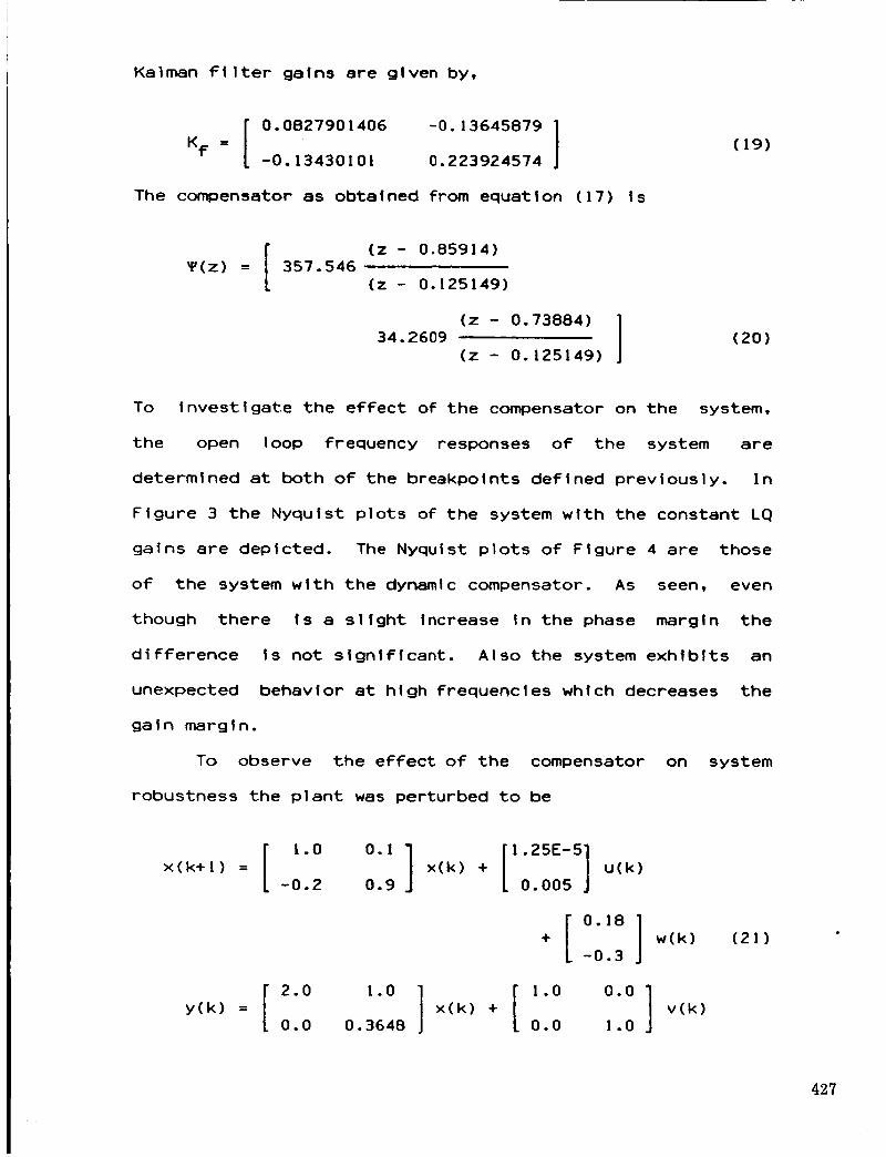
To Investigate the effect of the compensator on the system,

the open loop frequency responses of the system are

determined at both of the breakpolnts defined previously. In

Figure 3 the Nyqulst plots of the system with the constant LQ

gains are depicted. The Nyquist plots of Figure 4 are those

of the system with the dynamic compensator. As seen, even

though there Is a slight Increase in the phase margin the

difference ts not significant. Also the system exhibits an

unexpected behavior at high frequencies which decreases the

gain margin.

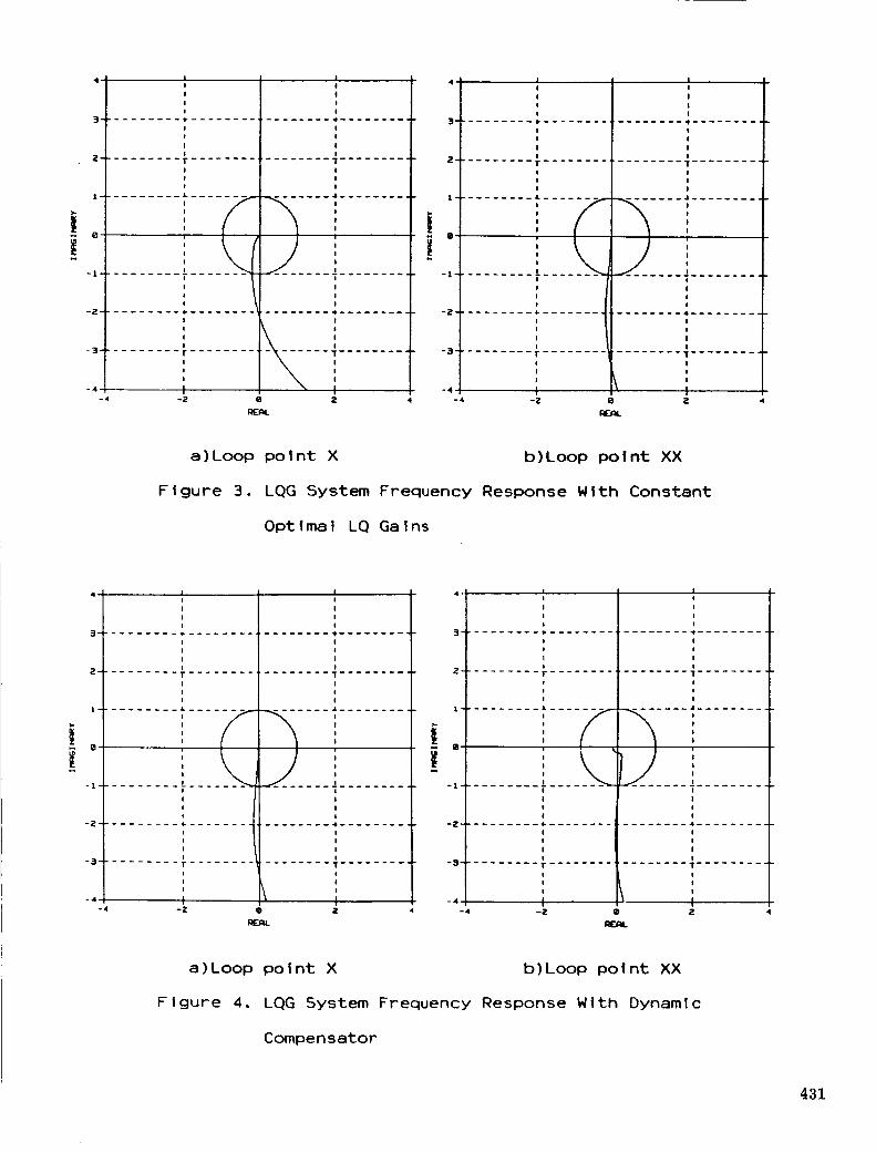
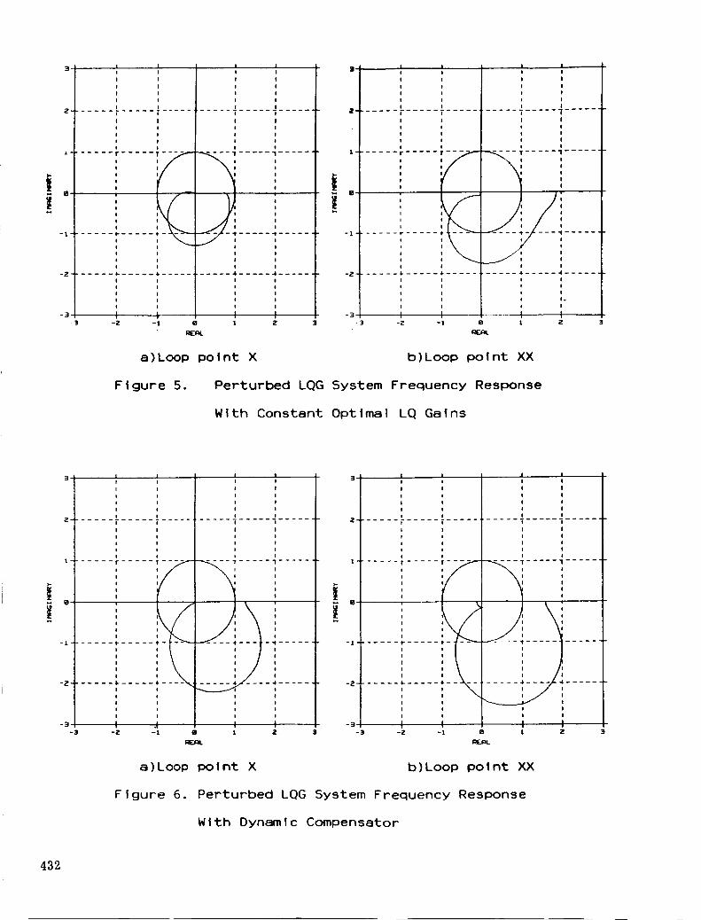
To observe the effect of the compensator on system

robustness the plant was perturbed to be

1.0 0.1 ]x(k+l) = x(k)

-0.2 0.9

2.0 1.0 ]y(k) = x(k)

0.0 0. 3648

+

+

! .25E-5] u(k)o. 005 J

+0.18 ] w(k)-0.3

1.00.0

0.01.0] v(k)

(21)

427

The Nyqulst plots of Figures 5 and 6 as obtained for

the open loop responses of the system with and without the

dynamic compensator indicate that the effect ts not

significant, but that there ts definitely an improvement. As

seen from Figure 6 there Is an Improvement in both the gain

and phase margins,at the plant input, i.e., the loop breaking

point XX. However at point X there fs a decrease in the gain

margin while a slight increase in the phase margin was noted.

The Following example demonstrates the fact that

although the compensator designed for the system is not

practically acceptable it recovers the stability margins at

the plant input of the LQG system. The plant Is the same as

the one given in (18) with the C matrix chosen to result in

The plant output is decrtbed by thean unstable controller.

following equation :

[° .01 [.000]y(k) = x(k) + v(k)

0.0 O.1 0.0 1.0

The Kalman Filter gains For this system are given by,

Kf = [ 0.143435809-0.23095458 -0.0624081382 ]0.10172081836

The compensator is described by,

• (z) = [-181195.7489

(z - 0.99095002)

(z + 565.52065)

-112641.206(z - 0.98813697)

(z + 565.52065)

The Nyquist plots of the system, with and without

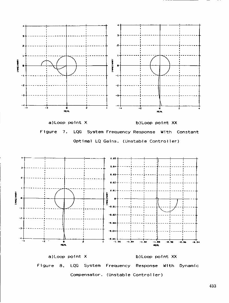
compensator are depicted In Figures 7 and 8. As seen

(22)

(23)

(20)

the

from

428

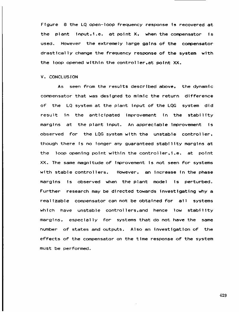
Figure 8 the LQ open-loop frequency response Is recovered at

the plant Input,I.e. at point X, when the compensator Is

used. However the extremely large gains of the compensator

drastlcally change the frequency response of the system wlth

the loop opened within the controller,at point XX.

V. CONCLUSION

As seen from the results described above,

compensator that was designed to mimic the return

of the LQ system at the plant Input of the LQG

the dynamic

difference

system did

result In the anticipated Improvement In the stability

margins at the plant Input. An appreciable Improvement ts

observed For the LQG system wtth the unstable controller,

though there Is no longer any guaranteed stability margins at

the loop opening point wtthln the controller,I.e, at point

XX. The same magnitude of Improvement ts not seen for systems

with stable controllers. However, an Increase In the phase

margins ts observed when the plant model Is perturbed.

Further research may be directed towards Investigating why a

realizable compensator can not be obtained for all systems

which have unstable controllers,and hence low stability

margtns, especfalIy for systems that do not have the same

number of states and outputs. Also an Investigation of the

effects of the compensator on the time response of the system

must be performed.

429

REFERENCES

[I] Doyle,J.C., "Guaranteed Margins for LQG Regulators," IEEE

Trans. Auto. Cont., Aug. 1978.

[2] Doyle,J.C., Steln,G., "Robustness wlth Observers," IEEE

Trans. Auto. Cont., Aug. 1979.

[3] Johnson,C.O., "State-varlable Design Methods May Produce

Unstable Feedback Controllers," Int. Jour. Cont., AprI! 1979.

[4] O'Rel Ily,J.,

Press, N.Y. 1983.

[5] Madlwal e,A.N.,

Transfer Recovery ,",

[6] Gupta, N.K.,

Observers for Linear Systems , Academic

Wllltams,D.E., "Some Extensions of Loop

ACC ,1985, pp 790-795.

"Robust Control/Estlrrw_tor Design by

Frequency-shaped Functlonals," IEEE Conf. on Dec. and Control

(CDC), 1981, pp 1167-1|72.

[7] Moore,d.B., Gangsaas,D., Bltght,d.D., "Performance and

Robustness Trades In LQG Regulator Design," IEEE CDC, 1981,

pp 1191-|200.

[B] Anderson,B.D.O., Moore,d.B., MlngorI,D.L. "Re latlons

Between Frequency Dependent Control and State Weighting In

LQG Problems," IEEE CDC, 19B3, pp 612-617.

[9] Okada,T., Klhara,M., Furlhata,H., "Robust Control System

wlth Observer," Int. Jour. Cont., May 1985.

430

i

A,

I-

0"

-I-

-2--

-3-

-4-

-4

I !I !

I l

! I

......... 9- ................ 4 .........i I

I I

! l......... T ........ * ........ I'.........

I I!

!

iiiiiiiiiii I

!

II

iiiiiiiiiiiiiI

I

! I........ I. ................. 4 .........

I

I

i

I

!

I

-2 IB

RF_¢_

!

i

I

I

II

I

I

, II I

I !

I I................. e- _ ................. .t

i i

i i

I Ii t

......... T ........ * ........ "I".........

!

!¢

iiiiiiiiiii II

B

!I

I

....... .JI ........

)i"I

II

I II I

I I

I /

I I

I I

' I-4 -2 Q 2

a)Loop point X b)Loop point XX

Figure 3. LQG System Frequency Response With Constant

Optimal LQ Gains

3-

2-

I-

0'

-l-

-2-

-3-

-4

-4

; II !

I II !

I !I I

I I

I I

I II I

I I

iiiiiiiiiiiii iiiiiiiiiiiiiiI I

I I

i I......... i- ................. 4 .........

i I

I II I

I !......... T ........ w. ........ ._ .........

i t

I !

I I

-Z • Z 4

, II I

I ii I

IIt ¢

I I

I I

! ii *

I I

.........!,,, ,,.........._ I I

! !

! !I I

- ........ ql-................. ,4.........

I II I

I I

I I......... 1"................. 7 .........

I I

' / 'I !! I

-4 -Z • 2

a)Loop point X b)Loop point XX

Figure 4. LQG System Frequency Response Wlth Dynamic

Compensator

431

I I3_

I I II

I I I I

I I i I

I I I I

I I I IZ' ....... F ..... T ........... _ ..... 3 ......

I I I I

¢ I I I

I I I l

I I I Ii I I I

_ ...... ; ..... ; ......--r ..... T ....

! i! l l o

i I l I

i I i !I I ! I

I I i I

I ii /I I I I /

li i I I! I I I

I I / /

I I I II I I i

i ! i II I I l

-3 1 I i I

-3 -Z -1 la 1 2 3

-1

.!

!; i , iI I ! !

I ! I I

I i i II I i I

I I i I --....... i" ..... T ..... _ ..... 'T ..... "i--"

I $ I lI i ¢ I

I I ! I

I I i Ii i i I

...... r ..... T ........ • ..... 1 ......

I I I I

i ' ' i, ,

: , , :i i ¢ I

i , , ,

i , I ,

i I

,, , _, ,,..... {,-..... 4-........... 4 ..... 4 ......

i I i I

i i i Ii i i ,

i i , ,.

I I ' I

I , I I

-3 -Z -1 el 1 2 3

a)Loop point X b)Loop point XX

Figure 5. Perturbed LQG System Frequency Response

With Constant Optimal LQ Gains

3 ; i ,I I I I

I i I ,I I , t

i , ¢ I

i i i ,

2 ....... r ..... T ..... _ ..... _ ..... _ ......I I I I

I I I I

I I I ,I I , I

i l i ii....... r..... T........ _..... I......

I i ¢ i

I i !

, , i I

I i , I

, , _ I ,

' tI , i II I i ,

-_ ...... I- ............. 4 .....

' ' _' ' /, , , i /

/I I I I

I i i ,I I l l

-3 , I I I

- -2 -I il 1 2 3

i• l l , o

I I I I

I I i I

i I I i

i i , II , , I

...... r ..... T .......... _ ..... ] ......

I ' I I

I I I I

I I ' 'I ' ' '

I I ' '...... r ..... T ........ • ..... "1 ......

i i l I

i I , ,i i , I

_ ' ,

i I I ¢i i I ¢

i i , ,i

...... I.-..... f ..... t" ...........

-,,," ,,,",,-2 ....... i-..... * ....... -_.... 4 .....

i

I I , I

i i I ,

I ' , Ii

-3 -_. -1 e l 2 t

EAL

a)Loop I_)lnt X b)Loop point XX

Figure 6. Perturbed LQG System Frequency Response

With Dynamic Compensator

432

4 L i 4 , _j

I lII

i I iI I

, I I I I

3 ................... T .................. 3 ......... _ ........ T ........ 4. .........

I I I I

2 .......... i ................ * ......... 2

I | I I

i I I I

, ,, ,0 e

1 ' '! !

t I'T --_.....-,'-_--':-- " ........._........ +................. T .............. _ .......

1 ' II '1 1 ' 'I I I I

-2 ........ _- ................ + .......... 2 ......... *" ............... + .........

1I I I I

I I I I

I I I I-3 ........ T ......... 3

........ "_ .................. I" ............... 1 .........

' / ' \I I I I

I I I I

-4 I I -4 I I

-4 -2 • 2 -4 -2 e 2 4

m£m/

a)Loop point X b)Loop point XX

Figure 7. LQG System Frequency Response With Constant

Optimal LQ Gains. (Unstable Controller)

4 , i j e 054 _ J+ .d-i i " I * I I

I I / , , iI I +4 I I II I _1, iB4 ..... t- ..... i ........... 4 ..... -4 ......

3 .......... _- ................. 4 ........ I I i I I

I 1 4 I i I I

I I I 4 I I

m i O.a:_ ..... r ..... I ..... 11 ..... "T ..... _ .....

' + -I ' ' 1 ' 'R .......... T ........ + .................. I i I *

+ * e {12 ' q * *

l I "I l l _ I I

_____ e.ml ..... 6. ..... , .......... .¢ ..... ._ .....

i l I l II I I I

+" i "1 i i IL i/--iI I I I

____, ......... e,81 ..... * ..... * .......... e .....

-I ......... _- ....... * / * i *

I I I I I I I

" t " "]-- i i t ii--+' ' ' '-_' .......... _" ............... 4 ......... I I I I

I I I I I II , I.I= ...............................

I I

-3 .......... r ............... 1" ......... ' * * *

I I e. Od I ..... I ..... I ..... I ..... t ..... I ......

l _ t l i I I I

I _ I I I I I I

-4 --Z • Z 4 -i. O6 -1.04 -I.0Z - 1. OO - •. 90 -I. 96 -•. 94

a)Loop point X b)Loop l_31nt XX

Figure 8. LQG System Frequency Response With

Compensator. (Unstable Controller)

Dynamic

433