n66 36859 - nasa o nasa contractor report no. 66109 gasl technical report no. 605 numerical flow...
TRANSCRIPT

Y
o
NASA Contractor Report No. 66109
GASL Technical Report No. 605
NUMERICAL FLOW FIELD PREDICTION
FOR PROJECT RAM-C "
By G. Widhopf, B. Kaplan and J. Jannone
Prepared for
National Aeronautics and Space Administration
Langley Research Center
Hampton, Virginia
NASI-5519
Prepared by
General Applied Science Laboratories,
Merrick and Stewart Avenues
Westbury, L. I., New York
Inc. I
June 30, 1966
N66 36859!
(ACCESSION ]NU ER)
',.(pAGES)
Ik _A GR ORrTMX OR AD NUMBER)
(THRU)
ODE)
|CATEGORY)
GPO PRICE $
CFSTI PRICE(S) $
Hard copy (HC)
Microfiche (MF)
ff 653 July 65
https://ntrs.nasa.gov/search.jsp?R=19660027569 2018-06-17T17:45:30+00:00Z

GASL TR- 605
Total No. of Pages - xii & 145
NASA CONTRACTOR REPORT NO. 66109
copy (81) of Ii0
By
NUMERICAL FLOW FIELD PREDICTION
FOR PROJECT RAM-C
G. Widhopf, B. Kaplan and J. Jannone
Distribution of this report is provided
in the interest of information exchange.
Responsibility for the contents resides
in the author or organization that pre-
pared it.
Prepared for
National Aeronautics and Space Administration
Langley Research Center
Hampton, Virginia
NASI-5519
Prepared by
General Applied Science Laboratories, Inc.
Merrick and Stewart Avenues
Westbury, L oI., New York
June 30, 1966 Approved by:
Anto_q FerriPresident

TABLE OF CONTENTS
TITLE
SUMMARY
INTRODUCTION
LIST OF SYMBOLS
ANALYSIS
Inviscid Field
One-Dimensional Inviscid Flow
Boundary Layer
METHOD OF CALCULATION
RESULTS
APPENDIX - Summary of Chemical Reactions
and Their Rate Constants
REFERENCES
TABLE I - RAM-C Flight Conditions
FIGURES
PAGE
1
2
4
7
8
9
l0
16
17
20
28
30
",31
ii

LIST OF TABLES
SUMMARY OF CHEMICAL REACTIONS AND RATE CONSTANTS
TABLE I - RAM-C FLIGHT CONDITIONS
21-27
30
iii

F IGURE
1
2
4-8
(4)
(5)
(6)
(7)
(S)
9-13
(9)
(i0)
(ii)
(12)
(13)
LIST OF FIGURES
RAM-C Vehicle Geometry
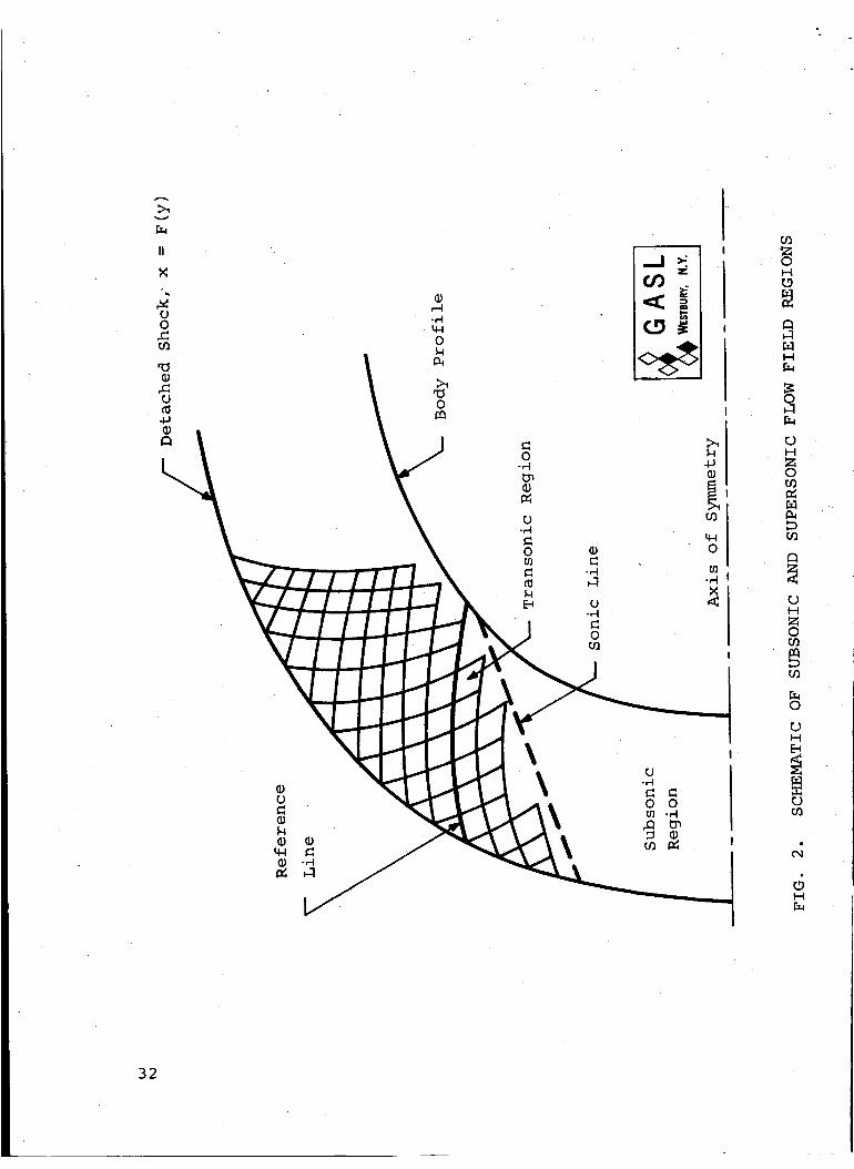
Schematic of Subsonic and Supersonic Flow
Field Regions
FlowField Schematic
NOMENCLATURE - Altitude = 36,800 Meters
Velocity Profiles at Surface Coordinate
Locations:
X=.09137, X=.I048, X=.1225 Meters
X=.1457, X=.1723, X=.1979 Meters
X=.3174, X=.4144, Meters
X=.6060, X=.8361, Meters
X=i.036, X=I.143, X=1.309 Meters
Temperature Profiles at Surface Coordinate
Locations:
X=.09137, X=.I048, X=.1225 Meters
X=.1457, X=.1723, X=.1979 Meters
X=.3174, X=.4144, X=.6060 Meters
X=.8361, X=I.036 Meters
X=I.143, X=Io309 Meters
PAGE
31
32
33
34
35
36
37
38
39
40
41
42
43
44

FIGURE
14-17
(14)
(15)
(16)
(17)
18-21
(18)
(19)
(20)
(21)
22-26
(22)
(23)
(24)
(25)
(26)
27-31
(27)
(28)
Electron Density Profiles at Surface Coordinate
Locations :
X=.09137, X=.I048, X=.1225 Meters
X=.1457, X=.1723, X=o1979 Meters
X=.3174, X=.4144, X=.6060, X=.8361 Meters
X=I.036, X=I.143, X=1.309 Meters
Specie Profiles (N) at Surface Coordinate
Locations:
X=.09137, X=.I048, X=.1225 Meters
X=.1457, X=.1723, X=.1979 Meters
X=.3174, X=.4144, X=.6060, X=.8361 Meters
X=I.036, X=I.143, X=1.309 Meters
Specie Profiles (0) at Surface Coordinate
Locations:
X=.09137, X=°I048, X=.1225 Meters
X=.1457, X=.1723, X=.1979 Meters
X=.3174, X_144, X=.6060 Meters
X=.8361, X=I.036 Meters
X=I.143, X=1.309 Meters
Specie Profiles (N) at Surface Coordinate
Locations:
X=.09137, X=.I048, X=.1225 Meters
X=.1457, X=.1723, X=.1979 Meters
PAGE
45
46
47
48
49
5O
51
52
53
54
55
56
57
58
59
v

F I GURE
(29)
(30)
(31)
32-35
(32)
(33)
(34)
(35)
36-39
(36)
(37)
(38)
(39)
40-43
(40)
(41)
(42)
(43)
X=.3174, X=.4144 Meters
X=.6060, X=.8361 Meters
X=I.036, X=I.143, X=1.309 Meters
Specie Profiles (0) at Surface Coordinate
Locations:
X=.09137, X=.I048, X=.1225 Meters
X=.1457, X=.1723, X=.1979 Meters
X=.3174, X=.4144, X=.6060, X=.8361 Meters
X=I.036, X=I.143, X=1.309 Meters
Specie Profiles (NO) at Surface Coordinate
Locations:
X=.09137, X=.I048, X=.1225 Meters
X=.1457, X=.1723, X=.1979 Meters
X=.3174, X=.4144, X=.6060, X=.8361 Meters
X=I.036, X=I.143, X=1.309 Meters
Specie Profiles (NO + ) and (e-) at Surface
Coordinate Locations:
X=.09137, X=.I048, X=.1225 Meters
X=.1457, X=.1723, X=.1979 Meters
X=.3174, X=.4144, X=.6060 Meters
X=.8361, X=I.036, X=I.143, X=1.309 Meters
PAGE
60
61
62
63
64
65
66
67
68
69
70
71
72
73
74
4
vi
FIGURE
44-46
(44)
(45)
(46)
47-48
(47)
(48)
49-52
(49)
(50)
(51)
(52)
53-55
(53)
(54)
Contour Maps - Altitude = 36,800 Meters
Pressure
Temperature
Electron Density
Pressure Profiles at Surface Coordinate
Locations:
X=.09137, X=.I048, X=.1225, X=.1457, X=.1723,
X=.1979 Meters
X=.3174, X=.4144, X=.6060, X=.8361, X=I.036,
X=I.143, X=1.309 Meters
NOMENCLATURE - Altitude = 53,500 Meters
Velocity Profiles at Surface Coordinate
Locations:
X=.01623, X=.03677 Meters
X=.I099 Meters
X=.1725, X=.2817, X=.4799 Meters
X=.6564, X=.8807, X=1.309 Meters
Temperature Profiles at Surface Coordinate
Locations:
X=.01623, X=.03677, X=.I099 Meters
X=.1725, X=.2817, X=.4799 Meters
PAGE
75
76
77
78
79
8O
81
82
83
84
85
86
vii

F IGURE
(55)
56-58
(56)
(57)
(58)
59-61
(59)
(60)
(61)
62-64
(62)
(63)
(64)
65-67
(65)
(66)
(67)
X=.6564, X=.8807, X=1.309 Meters
Electron Density Profiles at Surface Coordinate
Locations:
X=.01623, X=.03677, X=.I099 Meters
X=.1725, X=.2817, X=.4799 Meters
X=.6564, X=.8807, X=1.309 Meters
Specie Profiles (Ns) at Surface Coordinate
Locations:
X=.01623, X=.03677, X=.I099 Meters
X=.1725, X=.2817, X=.4799 Meters
X=.6564, X=.8807, X=1.309 Meters
Specie Profiles (0s) at Surface Coordinate
Locations:
X=.01623, X=.03677, X=.I099 Meters
X=.1725, X=.2817, X=.4799, X=.6564 Meters
X=.8807, X=1.309 Meters
Specie Profiles (N) at Surface Coordinate
Locations:
X=.01623, X=.03677, X=.I099 Meters
X=.1725, X=.2817, X=.4799 Meters
X=.6564, X=.8807, X=1.309 Meters
PAGE
87
88
89
90
91
92
93
94
95
96
97
98
99
viii

FIGURE
68-70
(68)
(69)
(7o)
71-73
(71)
(72)
(73)
74-76
(74)
(75)
(76)
77-79
(77)
(78)
(79)
80-81
(8O)
Specie Profiles (0) at Surface Coordinate
Locations:
X=.01623, X=.03677, X=.I099 Meters
X=.1725, X=.2817, X=.4799 Meters
X =.6564, X=.8807, X=1.309 Meters
Specie Profiles (NO) at Surface Coordinate
Locations:
X=.01623, X=.03677, X=.I099 Meters
X=.1725, X=.2817, X=.4799 Meters
X=.6564, X=.8807, X=1.309 Meters
Specie Profiles (NO + ) and (e-) at Surface
Coordinate Locations:
X=.01623, X=.03677, X=.I099 Meters
X=.1725, X=.2817, X=.4799 Meters
X=.6564, X=.8807, X=1.309
Contour Maps - Altitude = 53,500 Meters
Pressure
Temperature
Electron Density
Pressure Profiles at Surface Coordinate
Locations:
X=.01623, X=.03677, X=.1099 Meters
PAGE
i00
i01
102
103
104
105
106
107
108
109
ii0
iii
112
ix

F I GURE
(81)
82 -84
(82)
(83)
(84)
85 -87
(85)
(86)
(87)
88-90
(88)
(89)
(90)
91-93
(91)
(92)
(93)
x
X=.1725, X=.2817, X=.4799, X=.6564, X=.8807,
X=1.309 Meters
NOMENCLATURE - Altitude = 71,000 Meters
Velocity Profiles at Surface Coordinate
Locations:
X=.01623, X=.06126 Meters
X=.I1338, X=.1621 Meters
X=.5119, X=I.0077, X=1.309 Meters
Temperature Profiles at Surface Coordinate
Locations:
X=.01683, X=.06126 Meters
X=.I1338, X=.1621 Meters
X=.5119, X=I.0077, X=1.309 Meters
Electron Density Profiles at Surface Coordinate
Locations:
X=.01683, X=.06126 Meters
X=.I1338, X=.1621 Meters
X=.5119, X=I.0077, X=Io309 Meters
Specie Profiles (Ns) at Surface Coordinate
Locations:
X=.01683, X=.06126 Meters
X=.I1338, X=.1621 Meters
X=.5119, X=I.0077, X=1.309 Meters
PAG____EE
113
114
115
116
117
118
119
120
121
122
123
124
125
126

FIGURE
94-96
(94)
(95)
(96)
Specie Profiles (Os) at Surface Coordinate
Locations:
X=.01683, X=.06126 Meters
X=.I1338, X=.1621 Meters
X=.5119, X=I.0077, X=1.309 Meters
PAGE
127
128
129
97-99
(97)
(98)
(99)
Specie Profiles (N) at Surface Coordinate
Locations:
X=.01683, X=.06126 Meters
X=.I1338, X=.1621 Meters
X=.5119, X=I.0077, X=1.309 Meters
130
131
132
100-102
(!00)
(101)
(102)
Specie Profiles (0) at Surface Coordinate
Locations:
_= n1_ X= 06126 Meters
X=.I1338, X=.1621 Meters
X=.5119, X=I.0077, X=1.309 Meters
133
134
135
103-105
(103)
(104)
(105)
Specie Profiles (NO) at Surface Coordinate
Locations:
X=.01683, X=.06126, X=.I1338 Meters
X=.1621, X=.5119 Meters
X=I.0077, X=1.309 Meters
136
137
138
xi

F IGURE
106-108
(106)
(107)
(10S)
Specie Profiles (NO + ) and (e-) at Surface
Coordinate Locations:
X=.01683, X=.06126 Meters
X=.I1338, X=.1621 Meters
X=.5119, X=I.0077, X=1.309 Meters
PAGE
139
140
141
109-iii
(109)
(11o)
(IIi)
Contour Maps- Altitude = 71,000 Meters
Pressure
Temperature
Electron Density
142
143
144
(112)
Pressure Profiles at Surface Coordinate
Locations:
X=.01683, X=.06126, X=.11338, X=.1621, X=.5119,
X=I.0077, X=1.309 Meters 145
xii

NUMERICAL FLOW FIELD PREDICTION
FOR PROJECT RAM-C
By G. Widhopf, B. Kaplan, and J. Jannone
General Applied Science Laboratories, Inc.
SUMMARY
Detailed flow field calculations have been performed in
order to investigate the state of the gas in the shock layer
surrounding the RAM-C vehicle. Calculations were performed at
altitudes of 36.8, 53.5, and 71 km. For numerical purposes the
shock layer flow field was separated into an inviscid and
viscous layer wherein the viscous-inviscid interaction was
taken into account by a displacement thickness iteration pro-
cedure. A nonsimilar boundary layer approach was assumed to
be applicable in the viscous region where edge conditions were
computed by tracing non-equilibrium inviscid streamlines as
they were entrained by the boundary layer. Finite rate chem-
istry was computed throughout the entire shock layer. Detailed
plots of profiles of velocity, temperature, electron density,
pressure, and species mole fractions are presented at various
surface locations. The results indicate that this type of
computational procedure is not valid for this configuration
at the two higher altitudes.
INTRODUCTION
A series of flight experiments has been designed by theLangley Research Center in order to investigate the interfer-ence of the ionized flow field immediately surrounding areentry vehicle with radio transmission, communications andtracking. The official designation of these flight experimentsis Project Ram (Radio Attenuation Measurements). Utilizingthese experiments, coupled with detailed computations, methodswill be sought to eliminate the "blackout" phenomena. Also,assessments of theoretical analyses used in the prediction offlow field ionization and the associated RF signal loss will bepossible, since in-flight experiments have been included tomeasure specific reentry observables.
Project RAMhas been divided into specific flight experi-ments (RAM-A,B,C) where a spectrum of reentry flight conditionshas been investigated. RAM-A,B have been concerned with avelocity regime of 18,000 ft/sec and below, where various meas-urements and experiments have been made.
The RAM-C series consists of flight experiments at ahigher velocity regime (_ 25 kfps). Data from onboard sensorswill be transmitted in real time and recorded onboard for play-back after reentry. Tracking and telemetry data will beobtained throughout the flight. Experiments included in theRAM-C series are: onboard reflectometers, Langmuir probes,material addition schemes, thermocouples, multiple-frequency RFtransmission systems and antenna measurements. The RAM-Cvehicle has a payload of 200 pounds (see Fig. 1 for geometry)boosted to orbital reentry conditions by a four-stage Scoutvehicle launched from Wallops Island, Virginia, in the directionof Bermuda. The reentry data period starts after the fourthstage separation at an attitude of about 350 kft and continues
through the telemetry playback period which extends to below
50 kft. A beryllium heat sink nose cap will be used down to
about 160 kft, then expelled, and ablation heat protection used
for the remainder of reentry. A second payload using only
ablation heat protection will also be tested. It is likely that
Teflon will be the primary ablation material, with mass loss
expected to initiate at 200 kft or below. The payload will be
spin stabilized during reentry in an attempt to maintain a zero
angle of attack attitude.
2

The purpose of the study reported herein is to provide anumerical evaluation of the state of the gas in the shock layerbetween the vehicle surface and the shock wave envelope extend-ing from the nose region to the aft portion of the vehicle.This numerical investigation was carried out at the conditionsspecified in Table I.
Computation of the flow field about a blunted reentryvehicle of this type is a complex problem wherein the inviscidand viscous portions of the fluid field can interact to a highdegree. Certain restricting assumptions must therefore be madeto obtain a feasible line of approach toward a numerical solution.
Consideration must be given to the nature of the objectivesto be realized. The primary objective of the RAM-C program isto determine electromagnetic-fluid dynamic interaction. There-fore the most important feature will be to determine the magni-tude and spatial distribution of free-electron concentration inthe flow field.
A few conditions have been outlined to define the minimumrequirements needed and the general scope of the requirednumerical investigation. The gas in the complete shock layerflow is considered to be a multicomponent mixture of reacting
air species in the continuum flow regime. Radiation is to be
neglected as well as any angle of attack considerations. The
surface of the vehicle is to be considered as nonablative and
nonreactive, but is catalytic with respect to a non-equilibrium
reacting boundary layer. The surface temperature is constant
at a value of 1000°K while the flow near the surface is viscous
as well as reacting. The boundary layer is to be considered a
laminar region, where finite rate air chemistry, diffusion,
viscosity and heat conduction effects are taken into account.
Corrections should be made to account for momentum flux effects
(displacement thickness) and for inviscid flow vorticity.
3

LIST OF SYMBOLS
CP
Do •
_3
6c
_H
F
h
H
k
L
m
M
n
Ne-
P
Pr
r
R
eL_
specific heat at constant pressure, GM-CAL/G_K
specie diffusion term in energy equation
specie diffusion coefficient, C_/sec
species diffusion term in energy equation
enthalpy diffusion term in energy equation
characteristic function in finite difference notation
static enthalpy, GM-CAL/GM
total enthalpy, GM-CAL/GM
surface recombination coefficient, cm/sec
thermal conductivity, GM-CAL/CM sec ° K; Boltzmann constant
= 1.38032x10-s3 joule °K-z
body length, meters
finite difference mesh indicator
Mach number
finite difference mesh indicator
electron density, particles/meter s
pressure, Newtons/meter s
Prandtl number
local body radius, meters
free stream Reynolds number based on body length
4

Sc
T
U
V
V.1
1
X
Y
8
(
1,2
X
P
T
nose radius, meters
Schmidt number
temperature, 0K
velocity component in x direction, meters/sec
velocity component in y direction, meters/sec
diffusion velocity at wall, meters/sec
.thnet rate of production of the i specie, moles/cm s sec
surface coordinate, meters
coordinate normal to surface, meters
mass fraction, _ = D ./Dl
local bow shock angle, degrees
ratio of specific heats = Cp/C v
nondimensional ratio = (7 - 1)/(7 + i), boundary layer thickness
_0 - two-dimensional flowan index 1 axisymmetric flow
coordinates along and normal to body centerline
Mach angle, degrees
viscosity coefficient, _/CM-sec
kinematic viscosity; _ = _/D, cmS/sec
density, GM/C_
stability parameter for finite difference scheme
shear stress, GM/CM sec2; transformed coordinate = 2_/_
5

interaction parameter
stream function, GM/sec
Subscripts
b base
e boundary layer edge
i ith specie
sh shock
w wall
free stream conditions
6

ANALYS IS
In the situation where the Reynolds number is high, vis-
cous phenomena which occur in the flow field about a reentry
vehicle could be assumed, for computational purposes, to be
restricted to the boundary layer, enabling the inviscid and
viscous portions of the flow field to be calculated independ-
ently. If in addition, the Prandtl* and Schmidt** numbers are
on the order of one, a finite rate chemically reacting flow
field can also be separated in this fashion.
Separation of a flow field into inviscid and viscous
fields is dependent upon the condition that inviscid-viscous
interactions can either be neglected or accounted for in a
reasonable fashion. For conditions where neither of the above
is true a shock layer approach is necessary, wherein the entire
field is solved as a viscous region.
Viscous interaction effects can generally be accounted for
by an iteration procedure (when the Reynolds number is high)
whereby an apparent body is introduced to calculate the alter-
ation of the inviscid flow due to the presence of the viscous
layer. The apparent body utilized is the original body contour
plus the local displacement thickness as calculated from the
boundary layer flow. The entrainment of outer inviscid stream-
lines can be taken into account by the actual finite-rate-chem-
istry computation along these streamlines as they are "swallowed,"
and by the utilization of these computations to provide the vari-
able boundary layer edge conditions needed to compute the viscous
layer structure.
Due to the severe discontinuities in flow variables across
the curved bow shock and the resulting associated high tempera-
tures, ionization and dissociation phenomena are generally
important in the entire shock layer flow. Chemical considera-
tions are important in varying degrees in the inviscid region
where streamlines have associated with them a relatively higher
velocity and lower temperature (due to the decrease in curva-
ture of the bow shock) than those swallowed in the viscous flow.
*Prandtl No. _ Pr _ Cp_/k = viscous/thermal transports.
**Schmidt No. _ Sc _ _/PD = viscous/diffusive transports.18
7

Inviscid Field
The shock shape and the subsonic portion of the flow field
is computed by solving the elliptic Euler equations utilizing
the inverse method (Refs. 1-3). Here the body geometry in the
nose region is specified, and an initial estimate of the bow
shock shape is made by satisfying continuity conditions.
Characteristic lines are then constructed in the transonic
region (see Fig. 2) immediately downstream of the sonic line.
The characteristic line which extends from the shock and
terminates at the supersonic body point which is nearest to
the soni_c point, and subject to the condition that k < 1.0,
(k = sin i), is chosen as a reference line. The subsonic
portion of the flow field is then solved using the "inverse
approach" where the governing equations in the transformed
T,y plane are (Ref. 3)
Continuity
_¢ =_ p vx _¢ =p ubX p= u_ bY p= u
----y (i)
Momentum
u r +_-_ V - U 2 bY _ u
= 0
= 0
(2)
Energy
+ + (i + 8) 2u_
2_where Y = 7 ' and 8 = (y - l)/(y + i).
- 1 + [ (i - 6)/6M_ 2 ] (3)p8
8

Streamline entropy conservation
P p6
p_ '_Uco
= f(Ty s ) (4)
where f(TY s) is an arbitrary function determined by the shape
of the shock which maps into the line T = i.
The calculated profile of the nose between the axis of
symmetry and the point on the body common to the reference line
is compared with the given body profile. If deviations are
found the basic shock shape is automatically perturbed and the
calculation procedure described above is repeated until satis-
factory agreement is obtained. The gas is considered in chem-
ical equilibrium and includes the effects of gas dissociation
and vibrational excitation.
Conditions previously computed along the reference line
are utilized as initial conditions for computation of the
supersonic portion of the flow field. The familiar axisym-
metric rotational characteristic method is used assuming a real
gas in either chemical equilibrium or frozen flow. The program
has the capability of detecting discontinuities ±**_-the _-_--_u_
contour and therefore flow fields about body shapes containing
reentrant or expansion corners can be computed.
One-Dimensional Inviscid Flow
Assuming that non-equilibrium effects are small perturba-
tions on the basic equilibrium or frozen inviscid pressure
distribution as obtained from the inviscid solution described
previously, finite-rate chemistry can now be computed along
suitable streamlines.
A one-dimensional finite rate chemistry program (Ref. 5)
is used to compute the pointwise state of the fluid along
streamlines wherein all initial conditions and a streamwise
pressure distribution are prescribed. The analysis includes
the effects of vibrational relaxation in the chemical kinetics.
9

_0
The post shock conditions are solved utilizing real gas
thermodynamics whereas the species are considered frozen across
the shock. The governing equations are then integrated numeri-
cally along the specified streamline path utilizing these initial
conditions. Up to thirteen air species can be analyzed utilizing
up to thirty-nine air reactions. These reactions and their
associated reaction rates are specified in Appendix I. A com-
plete description of the analysis and the governing equations
can be found in _(Ref. 5).
Boundary Layer
The governing partial differential equations for the
viscous flow of a multicomponent chemically reacting gas mix-
ture are derived from the pertinent conservation laws with the
classical boundary layer assumptions (Ref. 4). The transfor-
mation of the boundary layer equations to von Mises coordinates,
X, _, is carried out to obtain a form more appropriate for
numerical solution. The stream function _ satisfies the con-
tinuity equation and eliminates the need for numerical inte-
gration of that equation. The transformation variable is
defined by
c (5)pur ( = 5-_ ; Pvr = - 5-_
where ¢ = 0 for two-dimensional flow and ( = 1 for axisymmetric
flow. The body coordinate X is retained in the equations to
simplify specification of distributions of body pressure and
wall conditions as well as to facilitate the tracing of inviscid
flow streamlines from shock to body stations.
The conservation equations take the following form in the
transformed plane:
i0

.e
Momentum
5u 1 dp + r --5X pu dX _
(e)
Energy
c 6c5X- r _--_ (6H + ) (v)
Species continuity (i = 1,2,3,...N)
_. -_.
- + r5x Pu 5@
(8)
"where T is the shear stress, 6H is the total enthalpy diffusion
term. 6c is the energy diffusion term due to species gradients,
is the species diffusion term and wi is the net rate of pro-
duction of the i th specie (Ref. 4). The diffusion velocity
resulting from gradients in the species distributions is assumed
to be specified by Fick:s law for a binary mixture and the lam-
inar viscosity is assumed to be given by the Sutherland law.
The reactions and their associated reaction rates are listed in
Appendix I where the reactions included in the analysis are the
first seven.
The equations are solved in the d,-__ a,_-F-_ _y inner
boundary conditions at the wall, outer edge conditions in the
inviscid flow which are unknown a priori, and the initial con-
ditions for property distributions through the layer at an
initial body station. The inner conditions at the wall and
distributions of initial conditions are specified as input to
the problem. The species distributions at the wall are assumed
known as a function of the effectiveness of the wall partici-
pating as a catalyst or a reactant in surface chemical reactions,
or are selected to be in local equilibrium.
ii

The catalytic wall assumption is as follows:
- P(_iVi ) = _P_i(9)
where KR = surface recombination coefficient and V. = diffusion
velocity at wall. i
For binary mixture
D 5O_.
i 1
• " BY K_ iR
(i0)
For fully catalytic wall, K R _ = for recombination of atoms and
"intermediate" molecular species. Therefore, for these species
m 0 at wall. For air there results
_02 = (_0_)"
= (XNz_N_ ( )_
at wall (ii)
all other _'s = 0.
The varying streamwise outer edge conditions are obtained
from one-dimensional non-equilibrium chemistry calculations
carried out along approximate inviscid streamlines from the
shock to the body station of interest• The air ingested in the
boundary layer by the swallowing of the inviscid flow is used
to determine the streamtube area at the boundary layer edge
(Fig. 3). Since the shock shape is specified data for this
portion of the problem,* the coordinates of the shock intersec-
tion point with the free streamtube are readily determined• At
that point all local post shock conditions are obtained from
*From the inviscid calculations, described above•
12

solutions of the shock equations with the assumption of frozen
species composition across the shock. The properties along the
streamlines, and thus, at the boundary layer edge, are then
determined for the chemically reacting air; where it is assumed
that the streamline pressure variation is of the same form as
the body pressure variation. The pressure level along each
streamline is uniquely defined by the post shock pressure and
terminating body pressure of each streamline.
Thus the conditions for solution of the problem (in the
absence of ablation) are:
X = X(0,_) ; u = u(Y) , H = H(Y) , _. = _. (Y)1 1
= @ (x,0) ;u = 0, v = 0, H = H (X), _. = _. (X) (12)W 1 lW
$ = $ (X,$e)', u = Ue (X) , H = H_ ' _'i = _'le (X)
• The deviations from zero slope condition at the outer edge of
the profiles (velocity, total enthalpy and species mass frac'
tions) beyond specified numerical tolerances are subsequently
used in the computer program to establish a call for new edge
conditions, via the forenoted streamline procedure.
The set of partial differential equations is reduced to a
system of algebraic equations for numerical solution utilizing
an explicit finite difference technique. The finite difference
form is developed by expressing the explicit difference rela-
tions for each of the dependent variables of the conservation
equations (the variable here denoted by a characteristic func-
tion, F) as follows:
_x - A x
(13)
13

_t _ = [a(X,_+ _-A _)
l A_)- a(X,_ --
2
{F(X,_ + A _) - F(X,_)] -
{ F(x,_) - F(X,_ - A _}3(14)
where
1
a(X,_ ± _ A _) _i [a(x,_) + a(x,_ • 4_)]2
The resulting difference equations are of the form
F(X+LiX,_) = A + B F(X,_) + C F(X,_ + A _) + D F(X,_- A @)n n n n
(15)
in which A, B, C, and D depend upon the equation (n index), the
coordinate, and the various air species.
The X,_ plane is divided into a finite mesh with grid
spacing of _ X and _ _, with nodal points denoted by intersec-
tions of lines m - i, m, m + i, and n - i, n, n + i, shown insketch.
n+ 1
n
n - 1
--A X--
m- 1 m m + 1
X
14
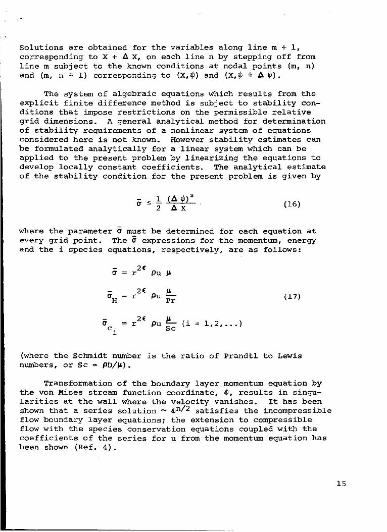
Solutions are obtained for the variables along line m + i,
corresponding to X + _ X, on each line n by stepping off from
line m subject to the known conditions at nodal points (m, n)
and (m, n ± I) corresponding to (X,_) and (X,_ ± _ _).
The system of algebraic equations which results from the
explicit finite difference method is subject to stability con-
ditions that impose restrictions on the permissible relative
grid dimensions. A general analytical method for determination
of stability requirements of a nonlinear system of equations
considered here is not known. However stability estimates can
be formulated analytically for a linear system which can be
applied to the present problem by linearizing the equations to
develop locally constant coefficients. The analytical estimate
of the stability condition for the present problem is given by
iX (16)
where the parameter _ must be determined for each equation at
every grid point. The _ expressions for the momentum, energy
and the i species equations, respectively, are as follows:
2E
_H = r Pu -- (17)Pr
2E= r
c.1
@u S_c (i = 1,2,...)
(where the Schmidt number is the ratio of Prandtl to Lewis
numbers, or Sc = PD/_).
Transformation of the boundary layer momentum equation by
the von Mises stream function coordinate, _, results in singu-
larities at the wall where the velocity vanishes. It has been
shown that a series solution _ _n/2 satisfies the incompressible
flow boundary layer equations; the extension to compressible
flow with the species conservation equations coupled with the
coefficients of the series for u from the momentum equation has
been shown (Ref. 4).
15

METHODOF CALCULATION
Described herein is the computational technique utilizedto investigate conditions at the three altitudes of interest.The methods used in order of application are:
(a) The inviscid flow field is computed for the basic
RAM-C configuration assuming equilibrium flow at the two lower
altitudes and frozen flow at the higher altitude. The analysis,
and the IBM 7094 program utilized, is described in Refs. 1 and 2
and in the ANALYSIS SECTION of this report. Results of this
program include the shock shape, and the tracing of inviscid
streamlines.
(b) The resulting shock shape and pressure distribution
serve as input to the non-equilibrium, reacting boundary layer
program detailed in Ref. 4 and in the ANALYSIS SECTION of this
report. Here the viscous region is computed utilizing non-
equilibrium chemistry and accounts for "swallowing" of vortical
inviscid streamlines. Among the parameters computed, the dis-
placement thickness is of immediate importance.
(c) Utilizing the resulting displacement thickness com-
puted from (b) a "corrected" body inviscid flow field is com-
puted (where the "corrected" body is the original shape plus
the displacement thickness). The resulting body pressure dis-
tribution is then compared to that pressure distribution which
was used in the previous boundary layer calculation. If there
is serious disagreement, step (b) is repeated. Steps (b) and
(c) are repeated until agreement in the pressure distribution
is reached. We then proceed to step (d).
(d) Non-equilibrium chemistry along streamlines in the
inviscid flow field is computed using the analysis described
in Ref. 5. Here the chemistry package utilizes ii species
and 22 reactions accounting for vibrational relaxation where
the species are considered to be frozen across the bow shock.
16

RESULTS
Detailed plots of the results obtained are shown in
Figs. 4-112. Profiles of velocity, temperature, pressure,
electron density and specie mole fraction have been plotted
at various stations along the body surface. Contour plots
of electron density, temperature and pressure are also in-
cluded for each altitude of interest. The results have
been divided into sections, according to altitude, with a
separate cover sheet describing in detail the nomenclature
utilized on the enclosed figures.
The complete profiles in the shock layer are depicted by
solid or dashed lines while the points illustrated by symbols
pertain only to the inviscid field calculations. The curves
represent computed values where no interpretation has been
impressed on the graphical presentation.
It is noted that the various chemical species are shown
approaching their respective free stream values which is con-
sistent with the concept of a thin shock (i.e., frozen species
across the shock). Thermodynamic and fluid mechanical quan-
tities approach values which are very near perfect-gas shock
_ .... m_ _ ...... _ _m1_n_ chemistry_ program
accounts for finite vibrational relaxation times, and immed-
iately behind the shock the vibrational mode has not been fully
excited, hence the near perfect-gas results.
Examination of the results poses some interesting questions
as to the feasibility of the approach utilized and interpreta-
tion of the results. It is therefore necessary to investigate
the assumptions and procedure used.
In order to obtain a feasible approach to a numerical
solution of the state of the shock layer flow certain initial
assumptions were necessary. A boundary layer approach was
taken to be feasible if modifications were made to compute
variable edge conditions and account for viscous interaction.
An iteration procedure was utilized whereby the viscous and
inviscid flows were perturbed until agreement was reached on
the body pressure distribution. The validity of this assump-
tion is contingent upon the degree of these interactions. The
17

interaction parameter X (Ref. 6) is indicative of pressure andviscous interaction, where
S_
(18)
For altitudes of 71, 53,5, and 36.8 km, X has the values 2.17,m
0.53, and 0.19 respectively. Values of X _ 0(i) represent condi-
tions where strong interaction effects should be taken into
account.
It would be expected, then, that the results of the lower
altitude calculations would be acceptable whereas the results
of the two higher altitude cases would be open to doubt. This
situation was, in fact, borne out by the results. The results
of the 53.5 km case were marginal and those of the highest
altitude case (71 km) were completely unrealistic.
Results of the 36.8 km case are presented in Figs. 4-48.
The match between the two solutions is reasonable. The curves
shown for this case represent the type of results attainable
from this type of computational procedure.
The mismatches between the viscous and the inviscid
results at the boundary layer edge (for any streamwise station)
are due largely to the arbitrariness associated with picking
an edge streamline. At any given station an edge streamline -
and thereby the complete state at the edge of that station - is
chosen by matching the mass flow in the boundary layer with an
inviscid streamtube in the free stream; i.e. the radius of the
inviscid streamtube, _ _, is chosen so that the mass flow_ _ sn
matches that in the moundary layer.
[ s° ]= 2 Pur (X) dY
@_u _ o
½
(19)
The arbitrariness comes, of course, in the choice of 6, wherein
the resultant streamline (defined by _ sh may be relatively hotor cool depending at what portion of t_e curved bow shock it
originated. Therefore computation of the edge conditions is
18

dependent upon this edge definition as well as the approximate
technique used to trace the swallowed streamlines. The dis-
placement thickness is also dependent upon this edge definition.
The iteration procedure used to perturb the inviscid flow
becomes questionable when the displacement thickness is large,
since a fundamental assumption involved in the utilization of
this technique is that the boundary layer is only a small
perturbation on the inviscid field. For the two higher alti-
tude cases the displacement thicknesses are large and thus the
mismatching between the inviscid and viscous solutions becomes
worse with increasing altitude.
Results of the 53°5 km case are presented in Figs. 49-81
where the streamline locations for the initial and final iter-
ations have been indicated° Successive iterations for the
71 km case resulted in boundary layer thicknesses larger than
the shock layer thickness and these results have been included
for the sake of completeness only, in Figs. 82-112.
At the higher altitudes the concept of a boundary layer is
no longer a realistic representation of the viscous layer about
the RAM-C vehicle. The classic assumption of a "thin" viscous
layer, fundamental in the derivation of the boundary layer
equations, is not valid and therefore the structure of the
viscous region as a boundary layer t_e flow is subject to
question. An approach whereby the entire shock layer is con-
sidered to be viscous must therefore be utilized to adequately
investigate the flow field properties at these reentry condi-
tions. This type of shock layer formulation, where non-equili-
brium chemistry is considered, is an interesting problem and
should be given future consideration.
19

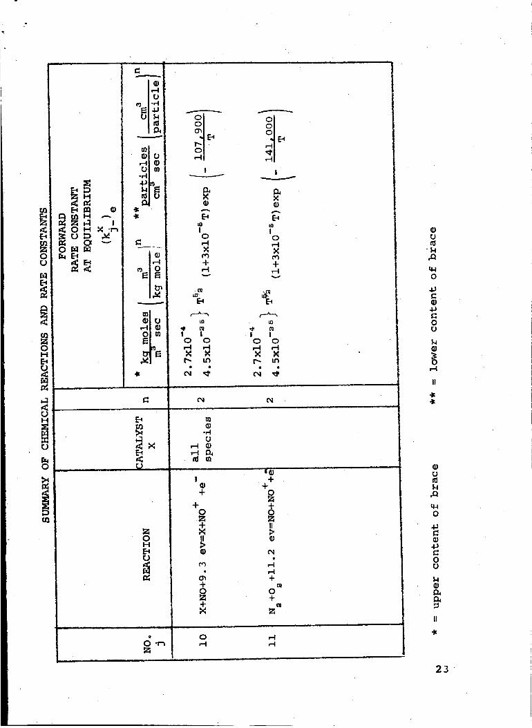
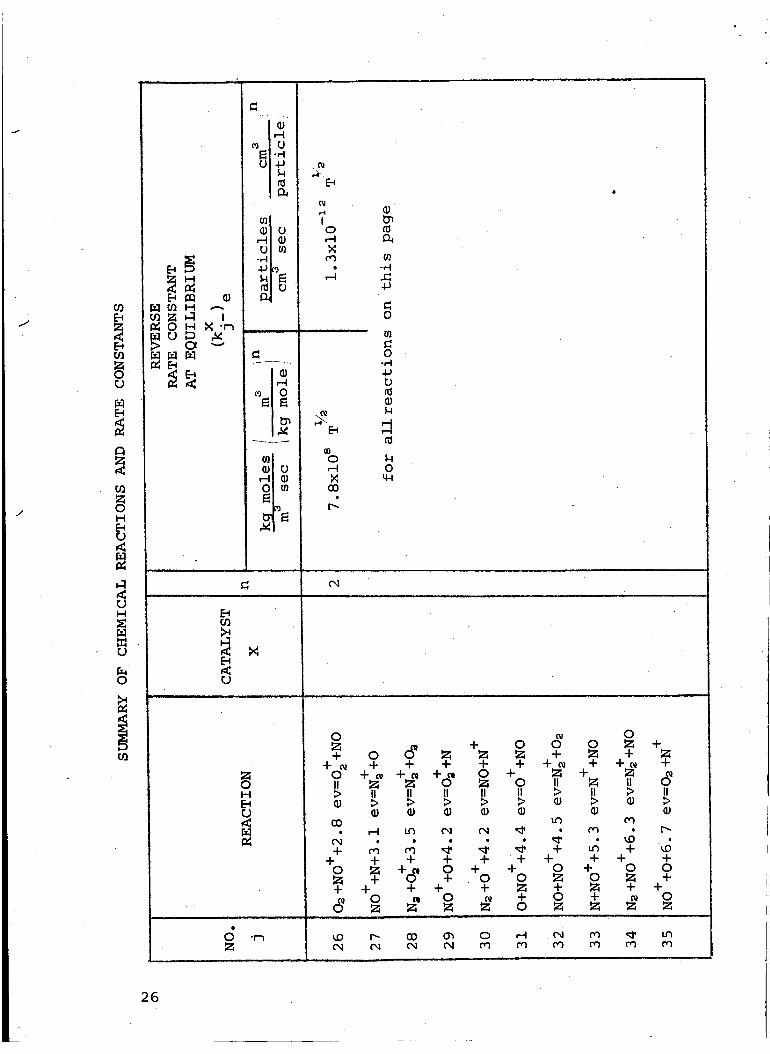
APPENDIX
SUMMARYOF CHEMICAL REACTIONS
AND THEIR RATE CONSTANTS
This appendix summarizes a large number of chemical reac-
tions which are significant at the high temperatures of reentry
into the earth's atmosphere at hypersonic speeds.
The presentation here includes two classes of units,
namely cm, sec, particle (used in Ref. 12) and meter, sec, kg
mole (required for the present analysis). The tables are self-
explanatory, though a word of caution is in order for the ioni-
zation reactions i0 through 15. The rate constants for these
reactions are tabulated as the forward (i.e. to the right)
values, which is contrary to the remainder of the appendix.
20

E_
ZOL)
V}
IM
U<
IM
O
O
{/)
C/) I.-I ,.-,
O _
t ....... L ,
C
U I-4 I I I I
I I I IQ) (3 O O O O
0 co X X X X
C
O
O
E i i i l
01 o 0 o 0
0 _ t_ 0 c,] 0
I
Io,-.4X
I
Io,-.4X
tD
p...
I
¢'1
IO
XO
I I
C0
IO IPl O
_D u_
I
m
IO_MX
e
I'N
C
[-t
H
O
O O
O
It>
Pl
+N+
,-_
0
I I I I I I
0 0 _' .t_
0 0 0 v,--I ,--I ,-I ,--I ,--I ,--I
CO ,-_ I"- 0 0
Z
Izl
II>
O0
o_+
.4-
_ ,-I I11
._ 4J0
<
0+
II>
u_
+
O
O ,-I III
_ 4J0
I0
p.
0
Xto
A
t_
+0
II>
e
+
4-0
21

z0O
ZOH
O
H
O
,--1 .i
i
I11,-4U
_ :.,4
ml• o
,-4 •O In
olai"
:OI,.- I
In• D
O tn
m
_ N
U
OH
O
_Z
O
I
_4O
Io
ouo
I
XO
o
X
A
O,OO
I
XO
I
X
o
I
I0
x
IE_
I0,--Ix
0
L_
I
c9
Io,-I
O I
oo
I
X0
#I
E_0
o,-IN
t
_ NN _
co o
A
I
o,-4
t'N t'M o,,1 o,,1 _
IO
0 +
_ _ ++ II _
II 111 II
_-I r,l
+ + OO +
I I• •
+ +
+
II II
• 11)
._n ,.0+ +
OO
q.4O
O.p
OD
O
O,-t
II
OU
u_O
1.4
22
0
,<
OH
,<UH
U
O
E.I I_1 •
0 "--"0_
O,..4
_ -__4J
rjm-r.I
O
_ OE E
t_Ol
II1Oi u
,-ti t[)
I ....
• I
o o0 oo'_ o
o _1',-I _1
I I ".
X
E_ E_U3 tO
I I0 o,--.IX X
+ +
19 I0
I I I I0 0 0 0
++
+
II
A+
+ _N _
O ,-4,..4 ,-4
I
+
+
0 II
I
I
0
0_J
,.-,I
U
O_J
,Cl
O
0
0U
0
II
23 ¸

U
0HE_
H
U
0
U ,-_O C_ "-"
II1,--I
!U
u I..l
I11 u,-4 d)U _n
-,-I-IJ_
Eni U
-It
,"-4
_1_
U
O CnE
t_E
OOO
,--4
,.-4
I
Nd_
in
Io
N
4-
I Io o,-.4 ,--IX N
p._ u'l
4
,.4 ¸
I
XI1)
lIB
Io,-IN
-I-
? Io o,--4 ,--tN N
O
(n
oiu_,--I
I •
N
t13
Io,-IN
-I-,--4
I Io o
X N
olo
,--4
N
A
Io,--tN
+,.-t
Ill
I IO, 0,'-I ,-4X X
4
u}
,-4 _ _-I -M
r_-IJ _ •O _
m
£--t
I-I
U
I
.t-
÷s+NII
,-4
,--t+
+N
,-I
ooo
,--t
Xi1)
Io,-4N
+,-t
110
I I0 0,--I ,-IN
CO
I I
+ +
+ &0+ -I-NII II> b
_0 _0
+ &0+ +
m
_ ,'_ ._0
I
+
--I-
ll
_o
u"l
+
-I--
©U
q40
0u
0
II
.I<-I<
u
q-I0
4_
0u
24

(/3E4
COZ0U
OH
<
<UH
O
T ,, , _
r_ r.II H A
H X "r"_
O v
C
,, I'-dU 4_
U
U _.,4 I4.1
C
Ill
_ 0
01_ u
,-4 I110 _
t_ _
I,,
U
OH
<
i
o,-tN
O,--t
t_r_
-H
4.1
0
C0
-,-I
ur_Ill_4
,-t,-4
Oq4
*sO +
o+ II +
O _> _E IIII _ II _>
O/o 0_++ o +
+
+ O+ O +
+ 00 0+ (_ + +
+ +_ ++ _
II 0 U II
I_ I> ¢) ¢)11)
,-I 0
+ _ + ++
+ +0z
to _- cO 0_,-4 r-4 ,-4 ,-4
0 ++ c_ +0 _ 0
+
+ O+_ ÷
Ill
+ M+ +
o +_+O +
25
J
oO
¢1
oI-I
8I--I
O
0
_ t
,--I
O 4-1
flJ
_n
•_ I.0¢II;0
,-4o_ 0
O
0 _n
0
0I-4
U
Ol
7o
X
J
0
i _
i
I, ,,, ,, ,
O_tOC_
In.r-I
.p
0
In
0.,--I.pD
r_
o
,, , ,,,, ,
,, ,, ,,, ,,, ,,, , , , ,, ........... , , ,i , ,, ,," , ....
0
o ¢+a/ + +
o + _ +_ +_II_> II II. II
_0• r-I I.D C_l Cnl
+ 4 _ 4 4+ + + + +
O Z +11 O +Z + O + O+ + + + +
O O 0_0 Z I_ l_i Z
(_ 0+ 0 0 0 Z +
Z + _ ++ + +0_ + +_/ +0 + Z + _ 0_Z 0 II Z II 0II II I> II l> II
I__* 4 J# + _4 + j+ + + + +
+ O + O OO Z O l_i +Z + I_ + ++ O ÷ 111 OO I_ Z I_ Z
_.D r_ GO O_ O ,.-4 o,_ _'_ _1'
,.. H
26

0
r.d
r_
ZoIM
U
=_.=.w=...--.-=-
c_ -_
+ @0 0
+ +I I0 0
II II_> _>• •
t_ coco
• co
+0 0+ +0 0
29

REFERENCES
lo
o
o
o
.
o
.
•
•
i0.
Lieberman, E., Computer Programs and Analysis for Flow
Fields About Bodies in Hypersonic Flight - Air in Chemical
Equilibrium and Frozen Flow Chemistry, GASL TR-460,
September 1964o
Lieberman, E., Input Formats and Operating Instructions for
IBM 709/90/94 Computer Programs to Calculate Inviscid Flow
Fields, GASL TR-460A, September 1964.
Vaglio-Laurin, R. and Ferri, A., Theoretical Investigation
of the Flow Field About Blunt Nosed Bodies in Supersonic
Flight, JAS, Vol. 25, pp. 761-770, December 1958.
Galowin, Lo So and Gould, H_, A Finite Difference Method
Solution of Non-similar Equilibrium and Non-equilibrium
Air, Boundary Layer Equations with Laminar and Turbulent
Viscosity Models, Part I - Analysis, Part II - Computer
Program and Supplement, Part III- Input Manual, GASL
TR-501, February 1965.
Gavril, B. D., Generalized One-Dimensional Chemically
Reacting Flows with Molecular Vibrational Relaxation, GASL
TR-426, January 1964o
Lees, L., Recent Developments in Hypersonic Flow, Jet
Propulsion, Vol. 27, ppo 1162-1178, November 1957.
Lin, S. C. and Teare, Jo D., Rate of Ionization Behind Shock
Waves in Air, II - Theoretical Interpretations, The Physics
of Fluids, Vol. 6, No. 3, March 1963.
Whitten, R. C. and Poppoff, I. G., Ion Kinetics in the
Lower Ionosphere, J. Atmos. Sci., Vol. 21, No. 2.
Eschenroeder, A. Q., Daiber, J° W., Golian, T. C., and
Hertzberg, A., Shock Tunnel Studies of High-Enthalpy Ionized
Airflows, Cornell Aeronautical Laboratory Report No.
AF-1500-A-I, July 1962.
Zeiberg, S. L., Oxygen-Electron Attachment in Hypersonic
Wakes, AIAA Journal, VOlo 2, No. 6, ppo 1151-1152, June
1964.
28

ii.
12.
Lees, L., Hypersonic Wakes and Trails, Presented at 17th
Annual Meeting of the American Rocket Society, ARS
Reprint No. 2662-62, November 1962.
Steiger, M.H., On the Chemistry of Air at High Temperatures,
GASL TR-357, June 1963.
29

TABLE I
RAM-C FLIGHT CONDITIONS
Conditions
Geometric Altitude
m
ft
Relative Velocity
m/sec
ft/sec
Ambient Conditions
Pressure
N/m _
ibs/ft _
Temperature
0K
0R
Density
kg/m a
ibs/ft s
Velocity of Sound
m/sec
ft/sec
71,000
232,900
7913
25,960
Case Number
II III
53,500
175,500
7864
25,800
36,800
120,700
7425
24,360
4.735
.0989
215.8
388.4
--57. 644x10
51.63
1.078
268°5
483.3
--46.697x10
4.772xi0 4. 181xl0
294.5
966.2
328.5
1000.8
445.5
9.305
241.5
434.7
311.5
1022.0
The ambient conditions used for these cases are those found in
the following document: Anon.: U.So Standard Atmosphere, 1962.
NASA, U.So Air Force0 and UoSo Weather Bureau, December 1962.
SI Units are shown, followed by the corresponding English Units.
30

%
t_
rjH
!
H
31
...J
oo_
oF
0H
H
UH
0
U
0
0
OI-I
r.)
H
32

/
I-4
33

NOMENCLATURE
ALTITUDE = 36,800 METERS
The shock locations for each profile are indicated by
the short solid lines drawn along the normal coordinate.
Since the shock layer thickness increases with increasing
surface coordinate location, their identification is there-
fore self-explanatory.
The data points indicate the results of streamline calcu-
lations where the code utilized for each station is indicated
on each figure. The symbol _ indicates the post bow shock
entry angle of the streamline considered.
34

.014
.012
.010
O)4o
.008
4J
-,-I'u
0o .006
oZ
.004
.002
!
0 X =-09137
• x=.1o48
• X=.1225|
X = 1225 _h
X = .1048sh_--_ s_r
/
0
0 i000 2000 3000 4000 5000 6000
Velocity, Meters/Sec
FIG. 4. VELOCITY AT SURFACE COORDINATE LOCATIONS X=.09137,
X=.I048, AND X=.1225 METERS, ALTITUDE = 36,800 METERS
35

.035
.030
.025
.0204_
d.015
oou
.010
oZ
.005
O X =- 1457
• X =. 1723
O X=" 197c"
sh
/ X=.l£
sh
x=.=53°A
53 ° - X =. iz
65 °
I'C
.___,-0 i000 2000 3000 4000 5000 6000
Velocity, Meters/sec
FIG. 5. VELOCITY AT SURFACE COORDINATE LOCATIONS X=.1457, X=.1723
AND X=.1979 METERS, ALTITUDE = 36,800 METERS
36

.14
ooU
o
..12
.i0
.O8
.06
.04
.O2
,,
--X = .4144
_ sh
3i 250
g[35°
/
--X =. 31746so: 6s°
i
Ji
0 2000 40On 6000 8000
Velocity, Meters/Sec
0X=.4144
_X=.3174
T
i0,000 12,000
FIG. 6, VELOCITY AT SURFACE COORDINATE LOCATIONS X=.4144
AND X=.3174 METERS, ALTITUDE = 36,800 METERS
37

m
.4"O
00
,-I
0z
• 16
• 14
.12
•i0
•08
.06
.04
.O2
0
X=.8361
0 2000 4000
sh
{so
#=s3 t
[ 65 °
6000 8000
Velocity, Meters/Sec
X=.6060
OX=.8361
_X=.6060
10,000 12,0(
FIG. 7. VELOCITY AT SURFACE COORDINATE LOCATIONS X=.8361
AND X=.6060 METERS, ALTITUDE = 36,800 METERS
38

6
@-_
_D _q O__q_ O0 ,--t _'_
AAA
O00
m
I I
s_aW
O
AI!
O
i
! w
O
.AII
OOO
_D
O,O
I
AIIX
O_O
AI!
X
,--4
,-'4
U
O
IIx
U_
iu_
o4_ _n
ioo°H
-_. _oo0
,,,-i
o I>00
OOOc4
OOO
O C0 _O _ c_O O O O
'X 'a_uTp_ooD T_uz_o_
O
O
O_DO
r_U II
H
.<
0,_
H
39

-r4
ooo
_4
_4o
.016
.014
.012 ......
.010
.OO8
.006
(7i°|
71 °
.004
.002,
0 X=. 09137
Q x=. lO4S
• x=. 1225
lO00 3000
FIG. 9.
5000 7000
Temperature,
9000 ii,000 13,0(
O
K
TEMPERATURE AT SURFACE COORDINATE LOCATIONS X=.0913
X=.i048, AND X=.1225 METERS, ALTITUDE = 36,800 METE
4O

4-I
4-I
-,4_D
00
r-Inl
0
.O4O
.035
.030
.025 -
.020
.015
.010
.005 ,,
I I • I
Ox =. 1457
0x=.1723
0x=.1979
=. 1723
0
i000
FIG. i0.
2000 3000 4000 5000 6000 7000O
Temperature, K
TEMPERATURE AT SURFACE COORDINATE LOCATIONS X=.1457,
X=.1723, AND x=.1979 METERS, ALTITUDE = 36,800 METERS
41

I0
o
000
42

L
to tqr_ 0
Q0 ,_II I!X NO •
ooo
0
t'qII
QO.,
X
_0Z
0 00 H
U
O
O4.J H
_ .• OO4OoN _O
o ud
r_i u
m_
i-t
oo
,-4
0 H00
0

0"_
II IIX X0 •
I,-t
0
l--
---1%
6
,-t
II
L o _
II V
0
IIX
i
_-I _-I _-I 0 0 0 0
s_e_W '_ '_%EuTp_OOD T_m_ON
000
0 IIo Xu_
0
0
0 II
r_Z0H
0 Uu_ 0
ql H _0 _ _ _1o _ _0 ._ 0
_ 0 0
(D gO
0
0
r-"
GH
000,-_
0
44

n_ 00 Ln
o_ o oio _1 ,-4
," ," ,"N N N
OOQ
.J _i
or-ix
,-4 _g
I1"X
0,-t
X
_0
_ % oo
0
I I I _fio 0
s_N 'A '_euTp_ooD Ie_ON 45

46 q
II' II" II'
X X X
0,.00
o
o
o
-J _
vJ
p..
×r-4
o% .
-,.-I
o
0
,---t
i
r..)_
X,-.4

_.j >:
_o_ _D_O
><><
cq,-4 ,-4
sla_W 'A
• o.'a_uzpaooD I _UXON
b
o
O
H
_7

48
0o ,,_ oo,--I(','1
II II IIM N N
0@_
ICO _0
II,-I
%
/_'_ o
s_a_N 'A
__J >:
o0
o
/
IIX
o o o
'a_uTpxooD I_mXON
0_
oe
,-4
×,-H
e
C_Z<
_g,-4
IIM
frl
_g
X
o/¢'}
-t
X
II
aJ Z0
u H.,-i E-_
8
_ OO
_ UO
4-1 Uu <
o
<-o
_m
O _
al<
m
t-
,-t
,-4
o
_z,-I
H

.014
.012
.010
4_
>; .oo8
d
-,-.I
X=-1225---_
0 .006
71°
,004
i__ 650
X =. 1048
7
sh
O
sh
-------------0
sh
____---------_
ASL, _ tl_smu_'. N.Y.
0 X =- 0913"
_X=.I048
_X=.1225
0
.25
FIG. 18,
.35 .45 .55 .65 .75
Mole Fraction (N2)
SPECIE PROFILES (N_) AT SURFACE COORDINATE
LOCATIONS X=.09137, X=.I048, AND X=.1225 METERS,
ALTITUDE = 36,800 METERS
.85
49
.040
.035
.030 .....
.1723
•005 i
sh
sh
, ,,
sh
OX=. 1979
Ox=.1723
OX=. 1457
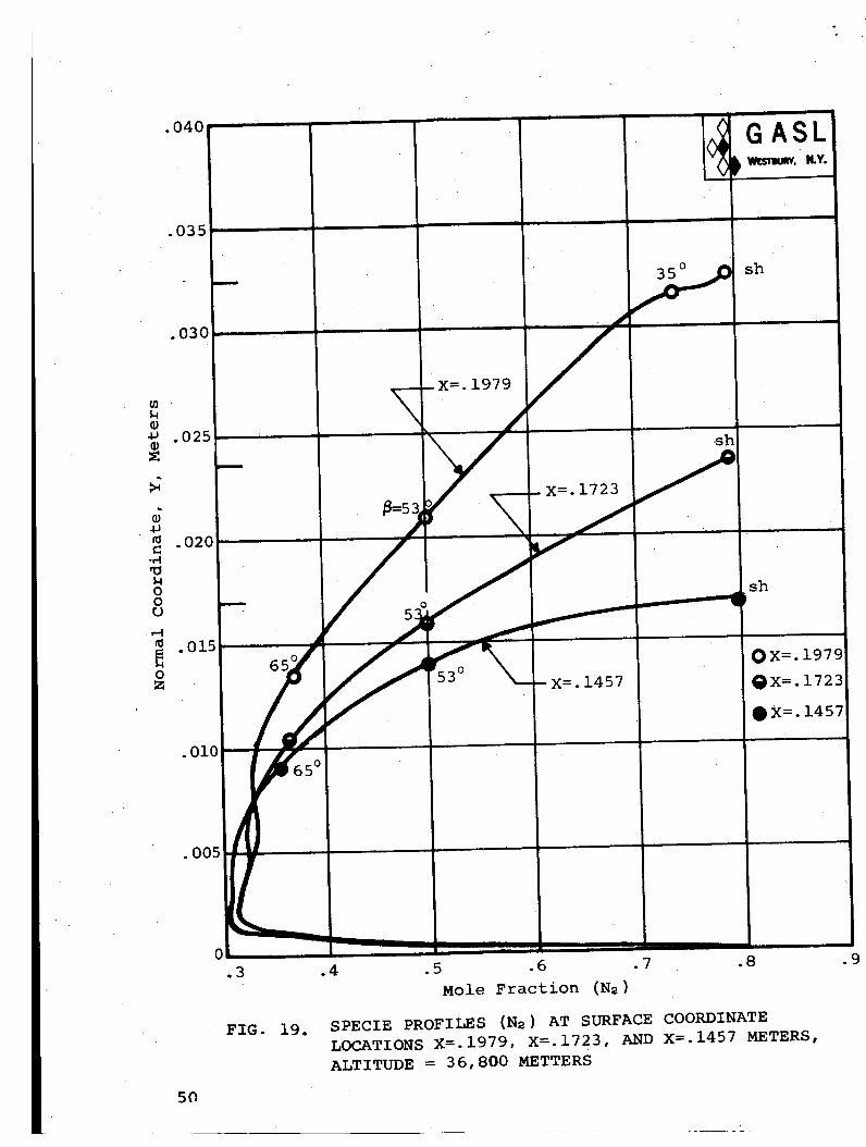
50 ¸
FIG. 19.
.4 .5 .6 .7 .8
Mole Fraction (N_)
SPECIE PROFILES (Ns) AT SURFACE COORDINATE
LOCATIONS X=.1979, X=.1723, AND X=.1457 METERS,
ALTITUDE = 36,800 METTERS
L _ _

E
-r4
00rO
,--4
E
0Z
.16
.14
.12
.i0
.08
•06
.O4
.O2
O X =- 3174
• X =. 4144
OX=.6060
"_,X=. 8361
_ G ASL) '_smum', ItY. ,1
_ sh
sh
X='8361 _ 25o
_ x:oo+o/_
x
IX_x=.3174
0
FIG. 20.
.4 .5 .6 .7 .8
Mole Fraction (N2)
SPECIE PROFILES (N_) AT SURFACE COORDINATE
LOCATIONS X=.3174, X=.4144, X=-6060, AND
X=.8361 METERS, ALTITUDE = 36,800 METERS
.9
51

.24
.22
.2O
• 18
• 16
14_) -
g .nm
.i0OOU
.4
08•
O
.O6
.04
.O2
m
m
m
O x:l.036Q x=1.143O X=l" 309
I
q_ sh
lJsh
250
,
65 °
X=l. 036
0.3
FIG.
.4
21.
GASL
.5 .6 .7 .8
Mole Fraction (N_)
SPECIE PROFILES (N2) AT SURFACE COORDINATE
LOCATIONS X=I.036, X=I.143, AND X=1.309 METERS,
ALTITUDE = 36,800 METERS
.9
52

I
t'-
,-4G_
O
ii°
M
O
,-4
O
1
(D u_
O e4,,-4 ,-4
,,. _"I_ 1,4
O0
X
CO I_
0 ,-I,-I O_
.1:: 0
I1" I_ II_
, ,, , ,,,,
Ji
nf.._
,-I
II
I It_ 0 013 _O _ c_-,-4 ,-I 0 0 0 0
0 0 0 0 0 0
sx_W 'A '_u_paooD I_UL_ON
O
O
,-4
,-4
O_
O
II'
°o x
Z
<
_a
O
_ _ -
,4
I
,-.t
0
53

t_
o.
54
Q
0 0
D
x
i_. c_
_-I',-I ,-I
," ,,","
000
(33,-I
Q
p..
,--t
ii°x
u_oq
I ,Iq R R'_ '_euTp_ooO T_oN
X
o
(_ JI'
_gp..,-I
u i,--4
,'-'t
II'
x
M
_0O_
-,.-I
U_
O0
r..)
X,-t
113
b
'o,--IX
,-4o
ul
v O:
O:
I--t _
_ ii I
al
UH
i-i

,-,It
oal
I|
I,
o,,D0_)
I"
0,-4X
%
55

O
II' II
O0
Q0
e
I I,-4 r-i
_0tOO
IIX
L
O
to
O
u'lto
i̧ i_ ,i_Ooh00
II'
CO
• I
r.i ,-t o o o o
OO,-I _OX to
,-4 O
II
oX _O
r-I t_CO
IIX
I H
oN O
O
_ H
o _• f'l .
_ 4.) 0I 0 0
0 rd U
0 _
m 00
0,-I (_o IIX "-"
I--t I-I
o_
N _ E.I
m _
_o,-4 H
O
56 sx_al4 'A 'aW_uTpxooD TEU_oN
II IIx
OO
I l
%
sxe_eN 'A 'o_uTpxooD T_mXoN
57

•016
.014
iii . .......i I
OX=.09137
QX:.lO48
_X=.1225
X=.1225
I I i I J
.002
0
0 .10
FIG. 27.
.20 .30 .40 .50
Mole Fraction (N)
SPECIE PROFILES (N) AT SURFACE COORDINATE
LOCATIONS ](--.09137, X=.I048, AND X=.1225
METERS, ALTITUDE = 36,800 METERS
.6O
58

o
D
.035
m
{_35 o
.03O '
.025
O X=. 1457
• X=. 1723
O X=. 1979
,,u
i i
_ /__x:1979
, i I015
• Ix=1723
OlO ,' i/
• _ x='1457 "_ i_GASL1'"" "".005
0
0 .i0 .20 .30 .40 .50 _60
Mole Fraction (N)
SPECIE PROFILES (N) AT SURFACE COORDINATE
LOCATIONS X=.1457, X=.1723, AND X=.1979
METERS, ALTITUDE = 36,800 METERS
FIG. 28.
59
4j TM
Z
00 04-
0Z
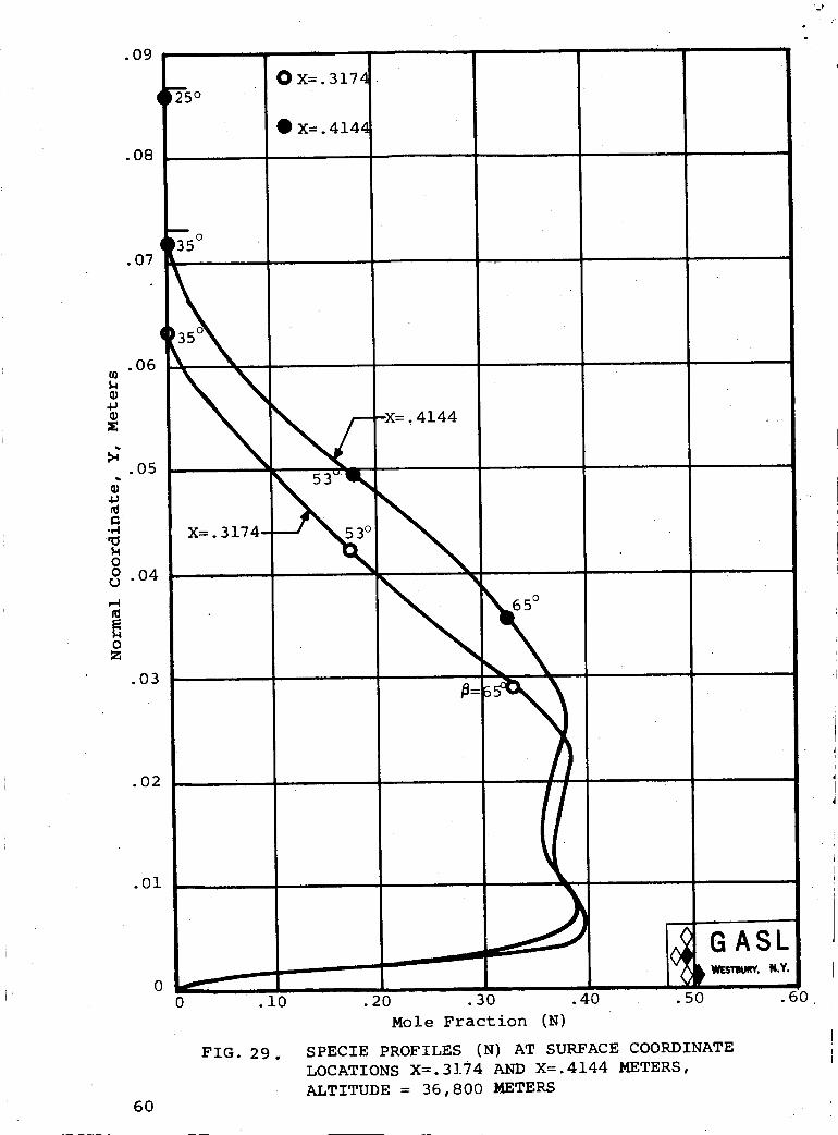
.O9
q_%o
.08
m
•07 (L_35o
• X=. 4144
.05
X=. 3174 ---J _
.O3
.O2
.01
0
6O
0
bIf
.i0
FIG. 29.
, n
.20 .30 .40 .50
Mole Fraction (N)
SPECIE PROFILES (N) AT SURFACE COORDINATE
LOCATIONS X=.3174 AND X=.4144 METERS,
ALTITUDE = 36,800 METERS
.60

e
•18
.16
.14
.12
.i0
4-*
.08
-H"O1.400C)
.o6
0
. O4
.O2
OX=. 6060
IK--.8361
i,
b25 °
I-- X=. 8361
0 ,.
0 .i .2
GASLW. ll._
.3
Mole Fraction (N)
FIG. 30. SPECIE PROFILES (N) AT SURFACE COORDINATE
LOCATIONS X=. 6060 AND X=. 8361 METERS,
ALTITUDE = 36,800 METERS
.6
61

_ o'_
o_1 _
II II IINN N
OOOi
I II,--t
m_
_ 0
S_ W '_
O
II m II
x Q.jx
II
/OO ',D0 0
'a_uTp_ooD I_tu_ ON
o o
o
u_
o
u_
A
Zv
0
oc,_ o•
0
Lr_
o
u%o
o
o
<
00O
0<
<
Z
H
Hr..)
m
H
O
IJN
,--40
Xm
- II
m _
o_
H_
O
62
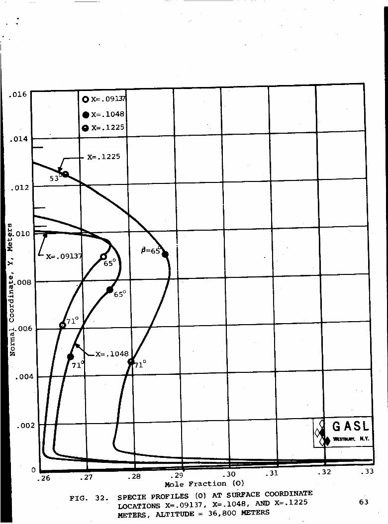
.016
.014
.012
.002
O X=. 09137
X=.1225
GASLWen'_. N.Y.
0
.26 .27
FIG. 32.
.28 .29 .30 .31
Mole Fraction (0)
SPECIE PROFILES (0) AT SURFACE COORDINATE
LOCATIONS X=.09137, X=.I048, AND X=.1225
METERS, ALTITUDE = 36,800 METERS
.32 .33 _
63
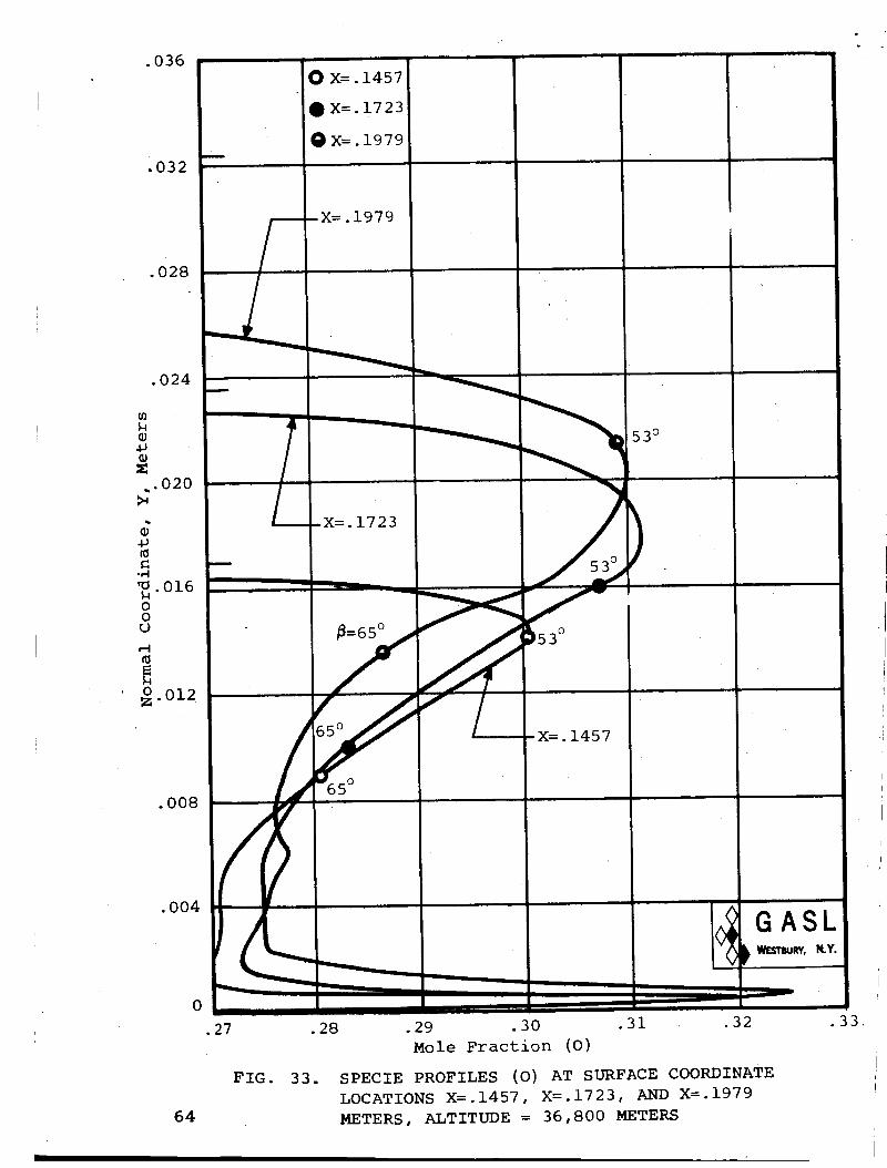
.036
.032
O X=. 1457
_X=.1723
Q X=. 1979
.028
.024
,.020
d
-,'-I'_ 016
00U
0 012Z"
.OO8
-X=.1979
-X=.1723
53 o
.004
o&64
.27 .28 .29 .30 .31
Mole Fraction (O)
FIG. 33. SPECIE PROFILES (O) AT SURFACE COORDINATE
LOCATIONS X=.1457, X=.1723, AND X=.1979
METERS, ALTITUDE = 36,800 METERS
GASLi,..,,.,.,,..o,,o_, .
.32 .33.

.16
.14
.12
.i04J
.o .08
00
•-4 .
0
.O4
.02
m
7
I0 X=. 3174
• x=.4144
i0 X=. 6060
_a x:.8361
_ X=. 6060
_X=. 3174
.24 .26
FIG. 34.
GASL
.28 .30 .32 .34
Mole Fraction (0)
SPECIES PROFILES (0) AT SURFACE COORDINATE
LOCATIONS X=.3174, X=.4144, X=.6060, AND
X=.8361 METERS, ALTITUDE = 36,800 METERS65

.4,-_
ooo
,--I
oZ
66
.24
.22
.20
•18
•16
•14
.12
.i0
•08
.06
•04
.02
O X=I. 036
Q X=I. 143
X=I. 309
X=l. 036
_ _"- X=I. 143
i- X=1.309
'__ 53o
g0.24 .26
FIG. 35.
.28 .30
Mole Fraction (O)
GASLWESTBURY,N.Y.
.32 .34 .36
SPECIE PROFILES (O) AT SURFACE COORDINATE
LOCATIONS X=i.036, X=i.143 AND X=1.309
METERS, ALTITUDE = 36,800 METERS
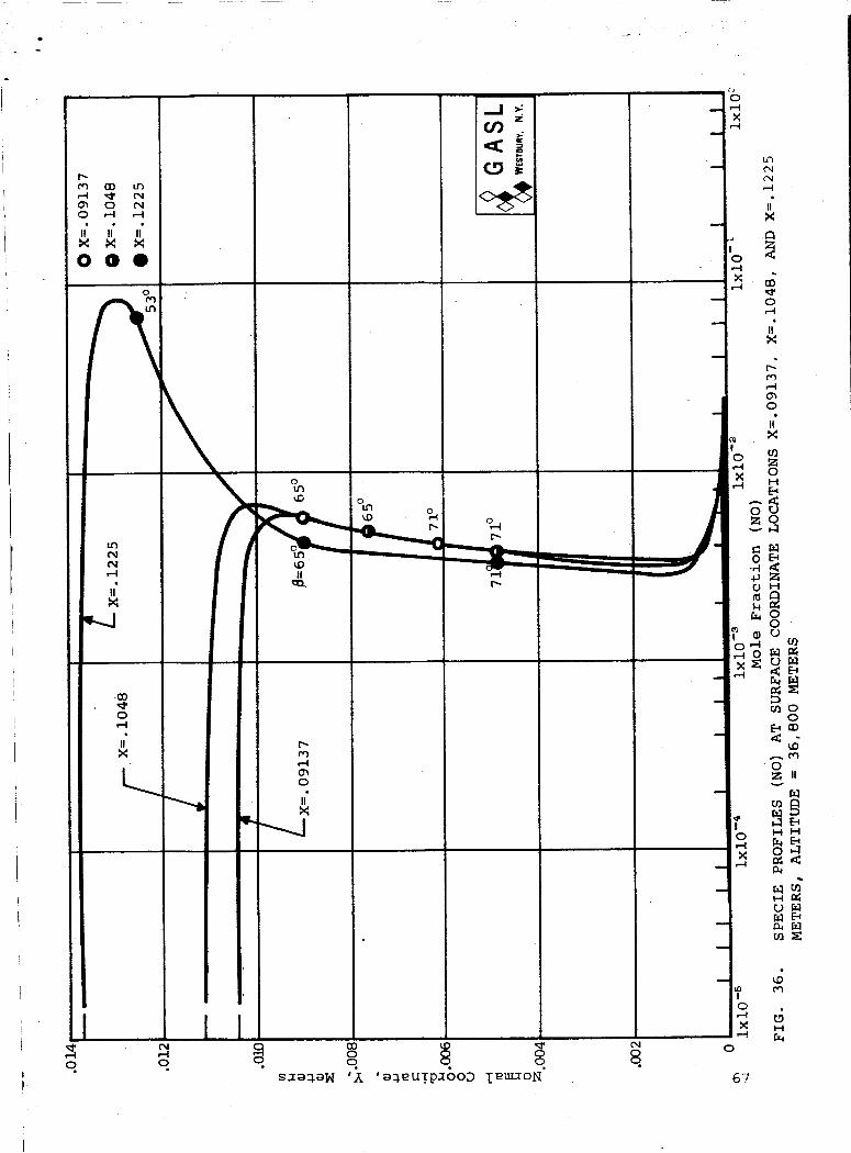
0
o.,..40
i
m
o
×
m
o o
sxa%eW 'A "a%euTpxooD leU_ON
cq
8
o
H
o
67

u%
68 q
u_ (-4
,-_ ,-4 ,_
ooe
\
r
z
oo
X,-t
o
,-t
o
o_ _ _ 0
q q o o qsleweW 'A 'e_uTpaOOD I_mXoN
--r-4
I
u0
I0
,-_X
o ,-4
ce)
i_--r-I
l.r)
II"
X
to
0I-I
t.)0
g
---o_0
0 o-,_ _ _0
_Ho__,
'H (J_ir..) ,-'1
m
6I--t

It
o
o_D
Ii° II
o o
69

P_
7O
_O
J
IIX
0_o
liX
O o
liN
o
U3II
O _ __ O O O
• I
s_a_W 'A '_EuTp_ooD IE_ON
o
of-4X
O_o
IIX
o
x,-.-II[N
,do
IIX
r/lz
oH
N U,--I _ O
O _Z
E-I
O-,-t H
u __ o_ o
IIJ r.r.1 _
X,-.-t r._ o
o
_ r¢)o
H H
O _,-4x _ad
m_
Io
M,--t
o
H
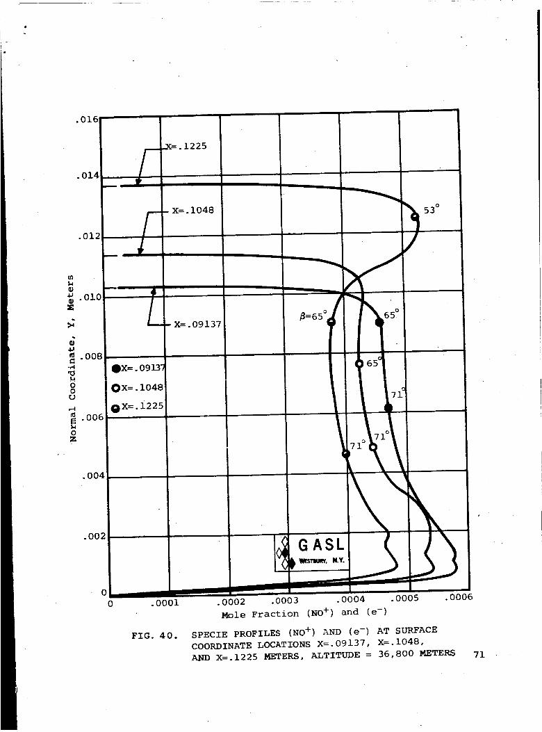
.016
.014
.012
010-
Z
G
.oo8-H
"0
00L)
006
oZ
• 004
.002
-X=. 1225
X=. 09137
OX=.0913_
OX=.I048
OX=.1225
650
o
71
53 °
q
7 c __
GASLII_s'rmu_, N.Y.
0
0 .0001
FIG. 40.
.0002 .0003 .0004 .0005 .0006
Mole Fraction (NO + ) and (e-)
SPECIE PROFILES (NO + ) AND (e-) AT SURFACE
COORDINATE LOCATIONS X=.09137, X=.I048,
AND X=.1225 METERS, ALTITUDE = 36,800 METERS 71

.040
.035
5oF-X=.I979
0
0 .0001 .0002 .0003 .0004
Mole Fraction (NO + ) and (e-)
SPECIE PROFILES (NO + ) AND (e-) AT SURFACE
COORDINATE LOCATIONS X=.1979, X=.1723, AND
X=.1457 METERS, ALTITUDE = 36,000 METERS
OK=. 1979
_(=. 1723
Ox=.1457
72
ASL_.smU_o N.Y.
.0005 .0006
FIG. 41.
] r

r.
X
.16
.14
.12
.I0
25
Ox=. 3174
E_X=.4144
QK:.6060
m
-,-4
.08
g _35 °
53a -x='3174
.02 _
J
0
0 .00002
FIG. 42.
.00004 .00006 .00008
Mole Fraction (NO + and e-)
SPECIE PROFILES (NO + AND e-)AT SURFACE
COORDINATE LOCATIONS X=. 3174, X=.4144,
AND X=.6060 METERS, ALTITUDE = 36,800
METERS
.00010 .00012
73

4J
oo
0z
• 24
.22
.20
•18
•16
•14
25 °.12
,25 °
OX=.8361
OX=l. 036
OX=I. 143
_X=I. 309
I
X=I. 036
X=.8361
X=i.143
74
_--65°.02
o0 .00002 .00004 .00006
FIG. 43.
•00008
Mole Fraction (NO + ) and (e-)
.00010 .00012
SPECIE PROFILES (NO + ) AND (e-) AT SURFACE
COORDINATE LOCATIONS X=.8361, X=I.036,
X=I.143, AND X=1.309 METERS,
ALTITUDE = 36,800 METERS

6,
a)
m
o6,
U
4
8
a_
- u,3
r_
,.D
C0
O
r:
r_
tJ
_4 z
.q o
f,l
_,_. _
_. _ .-, .-,,.,,-I
• ° ...... ° °
N_//e_ _ N&_NI(I_OOD _ON _I_OISN_IO-NON
d
o
o
75

oq
o
° ooo o
o oo
\o
ou_
o
6
r.. e_0
I
_._
U
o
o
Z
,.d
q
o
r_
8
o
r_
0
o
M
,.D
,4
o
un o o
gor'-
'.0 _ e.I 0 CO _O _' C',l 0 _lO _0 _ ¢',1 0 O0 '.O _1'
76 N_/_ 2 _ S._.VNI(]_OOD q%"_F_ON qVNOISN_4I(]-NON
o
co
_0
d
, oo

m

m
.032
.028
.024
ul
o
020-
= .016
o0U --"
,-4
E 012 "-.
o
•008
.004
FIGo 47.
78
OASL]K = . 1979
I I ,L
/
i
X=. 1723
X =. 1457
X=./225
. / / X =. i0/48
X =. 09137
/ ////', ///
4 8 12 16 20 24
Pressure, Newtons/Meter e x 10 -4
PRESSURE PROFILES AT SURFACE COORDINATE LOCATIONS
X=-09137, X=.I048, X=.1225, X=.1457, X=.1723, AND
X=.1979 METERS, ALTITUDE = 36,800 METERS

.16
.14
= .12
4J
- . 10Iii
-,.4
_ .oa,,-.t
0
.06
.O4
.O2
0
X=1.309r•X=I. 143
i X=I. 036X=.8361f
/.X=.6060
, ,| ,
X =. 4144
X=.3174
i
,i
G ASLi, ,,_,,,,,..,
0
FIG. 48.
1 2 3 4 5 6
Pressure, Newtons/Metez e x 10 -4
PRESSURE PROFILES AT SURFACE COORDINATE LOCATIONS
X=.3174, X=.4144, X=.6060, X=.8361, X=I.036, X=I.143
AND X=1.309 METERS, ALTITUDE = 36,800 METERS
79

NOMENCLATD-RE
ALTITUDE = 53,500 METERS
The shock locations for each profile are indicated bythe short solid lines drawn along the normal coordinate.Since the shock layer thickness increases with increasingsurface coordinate locations their identification is there-fore self-explanatory.
The data points indicate the results of streamline calcu-lations where the code utilized for each station is indicatedon each figure. The symbol _ indicates the post bow shockentry angle of the streamline considered.
The initial and final iterated streamline locations areindicated on the figures; where the squares indicate the initiallocations.
80

• 0O8
.007
OO6
005(D "
.004r
00
.003
0
.002
.001
0
0
FIG. 49.
|
O X =- 01623
• X =. 03677
I
ASL
sh
X=.03677----_
A
4---X=.01623
400 800 1200
Velocity, Meters/Sec
1600 2000 2400
VELOCITY AT SURFACE COORDINATE LOCATIONS X=.01623
AND X=.03677 METERS, ALTITUDE = 53,500 METERS
81

.016
.014
.012
,010
d .oo8
00
.006m
O
.004
.002
82
I i I i
00
FIG. 5 0.
J
65 °
O
77 °
nl
i000 2000 3000 4000
Velocity, Meters/Sec
VELOCITY AT SURFACE COORDINATE LOCATION
METERS, ALTITUDE = 53,500 METERS
s_=.i099
GAS.L_ Wl_r_mt. N.Y.
5000 6000
X = . 1099

ii"
I
,--IaO
000
E-,
ooo 0_cO 0_
ITM I_D ITM
,."4 _I _I'
OOO
, , -- q_ , g
o II- , " o X
C.'_
. • nn _'
o
r_
I11
o
III H
O -,.4O _ _,_ 0
..-,4.
1"4
ooo
0:0o
0o0
c,,l O CD _O,-'-4 ,--4 O O
I:o 0
sao_oN 'A 'a_uTpxooD T_m.xoN
oo
83
r.J9O_O_
t9<o_o
tel e,_
O_
H

oOr-4
84
0 I"
01oM
X
r_ _ o
OD u_ L_
It* I1'x
%%%_• I,
_.000,_ OOo')
o
II It II
Ir_
,Ic_,-4
s;[e_eW
0 0 0• , 0
a_ ,a_.TeuTp.,_ooD TEm.-co N
=.J >_
c/)
,.(.9
1
o
ooo00
ooop_
0oo
ooou_
ooo
ooom-)
0oo
ooo
o
o
O_0
II
0E)QO
II"
x
ii°
ul o
4-1
u'3
I'-t
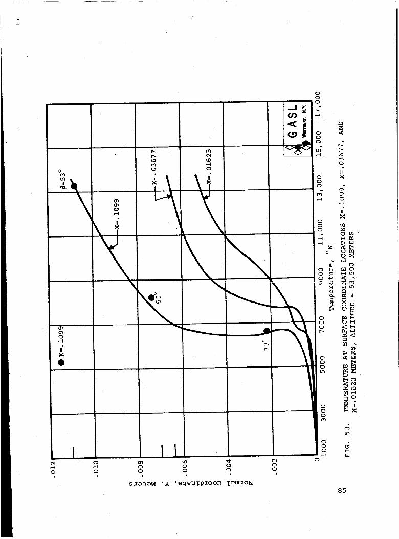
00
o
o
i II o _o H.... _
o _ _ _ _ o_ 0 o o o
0 0 0 o o o
8.5

p, r-,
II' 11' II°
II'X
00
II' ii°X
• 00o
<
o
o
II"X
o0
IIX
Zo o
I,-4 0 0 0
0
0 _ II'
0C_
u_
Io
000
0
H
sxeg, eW 'A 'eBeu_pxooD IeUL_ON
86

.18
.16
.14
.12
m.i0
40
O840 -m
.,4
oo{)
.06
oZ
. O4
.O2
i
!
0 X=. 6564
OX=.8807
"_X=I. 309
3_
35°I iI
-- X=I. 309
m X=.8807
X=. 6564
5_._ 5_ '
. 3 °
'__ G ASL
0
i000
FIG. 55.
2000 3000 4000 5000 6000 7000O
Temperature, K
TEMPERATURE AT SURFACE COORDINATE LOCATIONS X=.6564,
X=.8807, AND X=1.309 METERS, ALTITUDE = 53,500 METERS
87

O88 '
or--I
II"x
0
o
1 .-I
C/)
l
o,
o,
x
/ ilJ II :
o o 8. 0 0 0
s_e_eN 'A 'a%eu?p_boD TeUmON'
02
%
(D
.4
o
o
&
O4
,-4O
IIX
(3Z<
coo
II
8,
o_ ,.-4
O•,-4 H
_ O
_ H
OC O00
4..1O<r_ ul
o_o_tn
Zun
II
(.) H
,du'3
H

,-4
0 •
i °" X
If"
OD
o ,_ _
U
_4/ X._-_
0
/ _
m
co _o _ o_ o
_. _ o. o'A 'e:_uTp_ooD i_m_ON 89

r-I
9O
_o o 0u_ 00 oh
II' II II
o
,-.I

4_
44_m
-,4'0
00t5
,-4
0z
.016
•014
.012
•010
.OOB
.006
•004
.002
m
!
Ox=.01623
0X=.03677
OX=. i099
/
B=53 °
-X =. 1099
sh
"s_:-03677
. shX =. 01623
00
FIG. 59.
GASL_'mu_Y. N.Y.
.2 .4 .6 .8 .i0
Mole Fraction (Ne)
SPECIE PROFILES (N_) AT SURFACE COORDINATE
LOCATIONS X=.01623, X=.03677, AND X=.I099 METERS,
ALTITUDE = 53,500 METERS
.12
91

.16
.14
.12
.I0
d.o 08
i.looo
,-..t.06
O
.04
.02 --
0 _-
0
FIG. 60.
92
O X=.4799
QX=.2817
Qx=.1725
sh
--X=.4799
' 35 _35 °
_=53O sh
53°D i_
_-X=.2817
4_ . X=.1725
i
GASLWESmURY, N.Y.
.2 .4 .6 .8
Mole Fraction (N2)
SPECIE PROFILES (N2) AT SURFACE COORDINATE
LOCATIONS X=.4799, X=.2817, AND X=.1725 METERS,
ALTITUDE = 53,500 METERS
.12

m
4J
c
_o_4oorj
,--im
.24
.22
.2O
•18
.16
.14
.12
.i0
.08
•O6
.O4
.O2
0.3
FIG.
OX=.6564
O X=.8807
_X=1.309
53°_,
I X= I. 309 -
shJ,
:Il
X=.8807_._ p shsh
_=35° _ /
53°_ / /530_55°_
GASL
61.
.4 .5 .6 .7 .8 .9
Mole Fraction (N_)
SPECIE PROFILES (N2) AT SURFACE COORDINATE LOCATIONS
X=.6564, X=.8807, AND X=1.309 METERS,
ALTITUDE = 53,500 METERS93
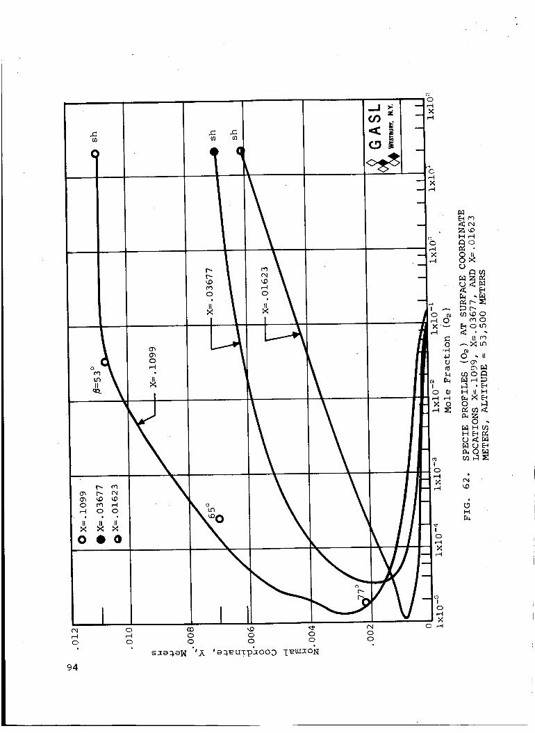
o
Ooo
0 E) O
o
o _ _ _o o o o
o o o o 0
s_e_a_ "A '_euIpaooD Te_oN
94
O_
o
,-4>¢
o eaO
X_
O
4au
_4
o
?o
To
>¢r-4
o,-4
Z<oH,-4
N _r,.) N
r_
m_Doe,._o
ii ¢,__Mm
o _. ii
t.r.1 ,-t _
H
o_Hd
NU_
m_
tD

95

o om
mAlJ* JlX X• 000
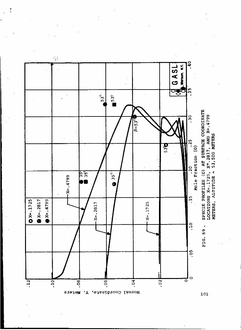
96
,--I ,-..4
h
O 0
ofel
O
O
-J_ o,-4 O
_ X
o.
0co
I. o o
N O
o
uh
OI ou3
01
otXl 0 CO _D _1',--I ,--I 0 0 0
I0 ¸,-I
_O
Io
' Xm
I
i
m I0,-_N
,-.I
E.t O
4
6H

.016
.014
.012
4_
:Z .010
4_
"_ 008-
oou
|w
o .006
.004
.002
O X=. I099
- X=. 1099
- X=. 03677
.
0 .i
FIG. 65.
.2 .3 .4 .5 .6
Mole Fraction (N)
SPECIE PROFILES (N) AT SURFACE COORDINATE
LOCATIONS X=.I099, X=.0367_, AND X=.01623 METERS,
ALTITUDE = 53,500 METERS 97

0 X=.4799
• x=.2817
• x=.1725
-X=. 4799
-X=. 2817
X=. 1725
98
0
0 .i
FIG. 66.
.2 .3 .4 .5
Mole Fraction (N)
SPECIE PROFILES (N) AT SURFACE COORDINATE
LOCATIONS X=.4799, X=.2817, AND X=.1725
METERS, ALTITUDE = 53,500 METERS
.6

X,-4
o
o0,-4X,-4
70,-4
x,-4
!0
Z
0
1.4P.4
0,-4o
,c0cO(D
II"
X
II"
x_
H O
8,;Om
_.1 I|
m [-4
_,1 ||_Nr_
Hr_
99

.016
.014
.012
4_
_ .010
.oo8
o
i .006
.004
i00
.002
i
O X =- I09S
X=.i099
ii i
- x=.01623 ___
0 _ __
.24 .25 .26 .27 .28 .29
Mole Fraction (0)
FIG. 68. SPECIE PROFILES (O) AT SURFACE COORDINATE
LOCATIONS X=.I099, X=.03677, AND X=.01623
METERS, ALTITUDE = 53,500 METERS
.30
i
b
•-4 O O• • • •
(2) z "
-,4
o_ _
I/3
p-
JlX
iio o
o
o
oo
0 . ii
r_
H
_Z
o d_H
_uEt
_ O_
6H
sxew_H 'A 'a_EuTpxooD I_XoN i01

•18
.16
•14
.12
0 35°
n
O X:. 656_
X.i0
D 35°• _ 35°
;_ .08
o --X=.8807
___=35°0 -X=.6564 . _53°C_53°
.06 __" ,,_a_ _53o
• O4
.O2
102
0 .05 .10 .15 .20 .25 .30 .35
Mole Fraction (O)
70. SPECIE PROFILES (O) AT SURFACE COORDINATE
LOCATIONS X=.6564, X=.8807, AND X=1.309
METERS, ALTITUDE = 53,500 METERS
FIG.

,-IO
m
w
O
L
Cr_0r-I
if °
",4
c_
II
0,-I0
0
I1"
X
0
O O OO O O
s_a_N "A '_u3p_ooD I_UL_ON
('W
OO
IO;-IX
,....Ix
;-.tX
AOZ
c:0
-,-I
U
,"4
'o,-4
IO,-IX
_ ,--4
!O,--I
X
O
',O
O
It"
X
<
,.2I".-
O
if"
X
O_O
ii °
X
ZOH
<uO
<ZH
L_
Dmo
o
._u3
0Z II
N_H H
_dH_U _
mN
H
103

u%eqr,-,-4
O
,-40
104
F--,-4co(',,i
I
O
0_o_r--
Q
o_o_r--
U__
,_ ,-4
o
,-.4
s_e_a_
¢N0 0 0
'A 'a_euTpa6oD lemaoN"
o
m
o
o,-4
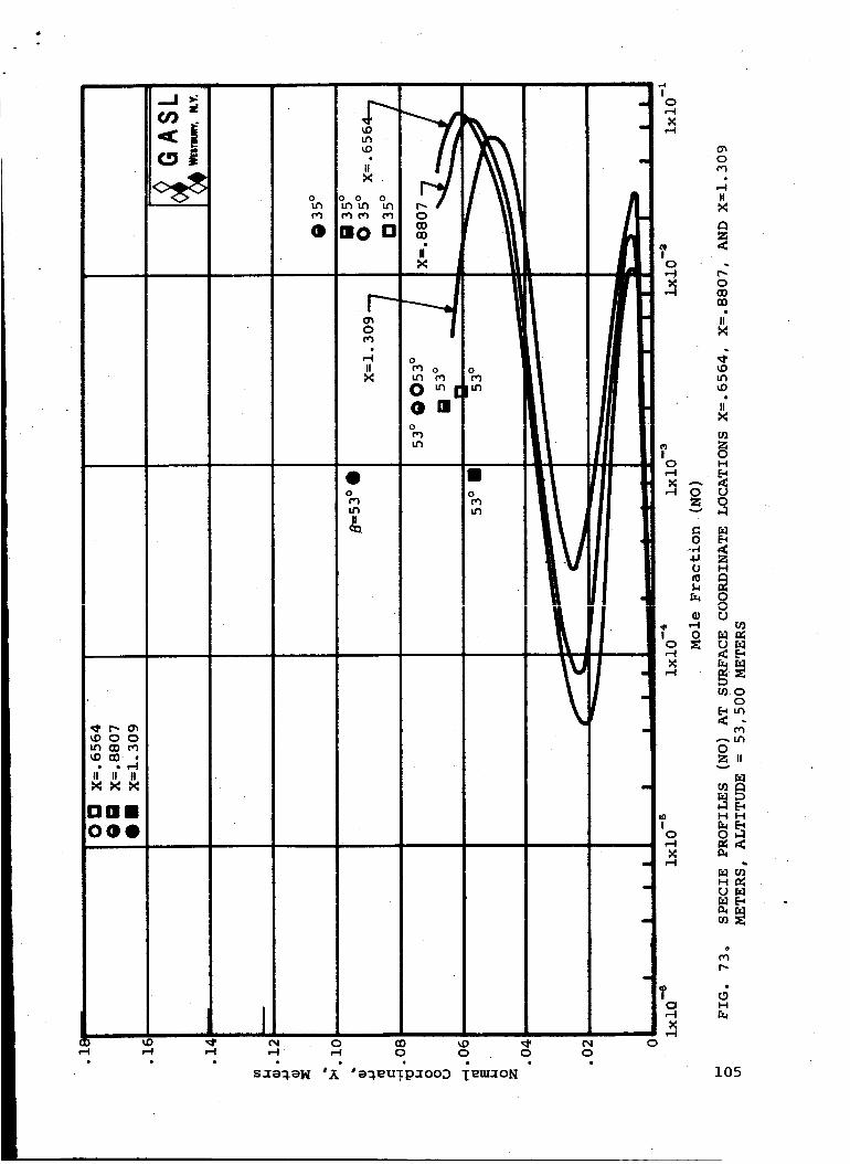
,_' r,,- o'_
II" I! IIXX_
DEll000
r-4 r_
omoD a)=i
N
F"-o
IIO
_ O O
0 _ £1_omo
• II0 iO
t/_ t.nII
,--4
I,-'1 f-I 0 0 0
• £ ip " "8.Z_N a aO_.eu. _[OOO "[RUL.'[ON
¢N0
.%,--IX
'= ,--I
m
tI
0
X,-j
c_
I0r-4
0
0.r4
Um
(1)
r-JI O
N• ,-.-t
o,,..4N
,-t
?O
X,,-t
O
o0el
IIX
1:1Z
o
_0
_D
t/3
M
O
[-4
H
O_m
O
H H
H_
Hr_
105

.016
.014
.012
0104J •
008-
0
,, •
--X=. 1099
o
006 _
--X='03677
.002
I _ --X = .01623
_oo_ / )
106
0
0 .0002 .0004 .0006 .0008 .0010 .0012
Mole Fraction (NO + & e-)
FIG. 74. SPECIE PROFILES (NO + ) AT SURFACE COORDINATE
LOCATIONS X=.I099, X=.03677, AND X=.01623 METERS,
ALTITUDE = 53,500 METERS
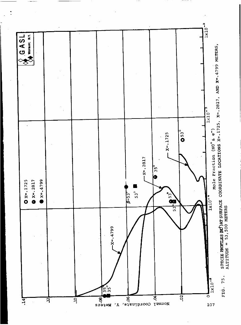
_DH_r..) H
o'_ o'1
sxe_eN 'A 'eWRuTpxOOD TenON
O
[-,.
_4
H
107
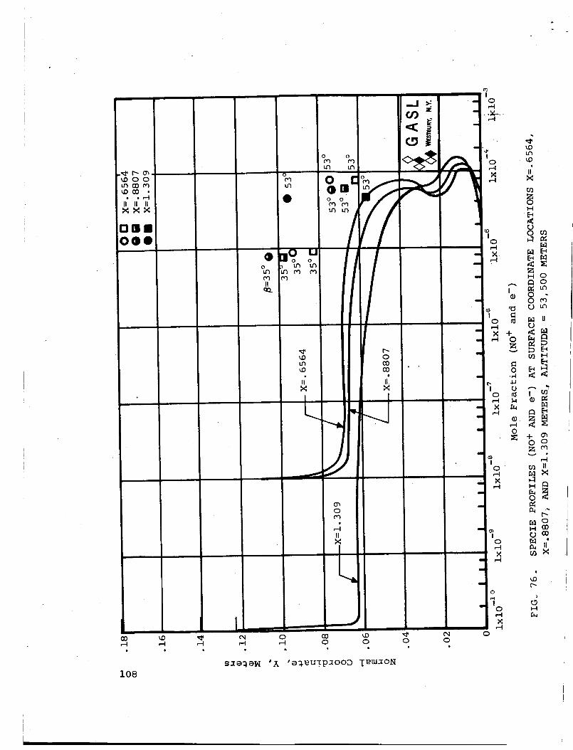
_oo
II° II II
xxx
,-I ,-I ,-,4• 0 •
108
o
AII
0 0


o
o _0
0
o_D
0
o
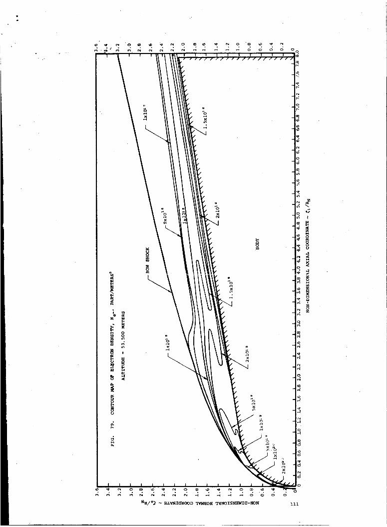
• • o • o
...., ° • .... • ° .

.,4
oorJ
,-I
•016
•014
.012
•010
•008
•006
m
i
X=. 1099
X='03677 I I X='01623
• 004
112
.002 ,
0
0 lO, 000
FIG. 80.
J20,000 30,000 40,000
Pressure, Newtons/Meter e
50,000 60,000
PRESSURE PROFILES AT SURFACE COORDINATE LOCATIONS
X=-01623, X=.03677, AND X=.I099 METERS,
ALTITUDE = 53,500 METERS

o
AJ
4J
--4
oo
.16
.12 --
.10
.O8
• O6
.O4
n
X=l. 309
X=. 8807
X=.6564
X .4799
fX =. 2817
//f
.O2
0
0 4000
FIG. 81.
X=.1725
GASLIn_mJ_o N.Y.
8000 12000 16000 20000
Pressure, Newtons/Meter _
PRESSURE PROFILES AT SURFACE COORDINATE LOCATIONS
X=.1725, X=.2817, X=.4799, X=.6564, X=.8807, AND
X=!.309 METERS, ALTITUDE = 53,50G METERS113
24000,
NOMENCLATURE
ALTITUDE = 71,000 METERS
These results have been included for completeness only.
The shock locations for each profile are indicated bytheshort
solid lines drawn along the normal coordinate• Since the shock
layer thickness increases with increasing surface coordinate
location, their identification is therefore self-explanatory.
The data pOints indicate the results of streamline calcu-
lations where the code utilized for each station is indicated
on each figure. The symbol _ indicates the post bow shock entry
angle of the streamline considered.
The solid lines on the enclosed curves represent the final
iterated boundary layer results. These profiles have been cut
off at the shock. The dashed lines represent profiles drawn
through the results of the inviscid calculations.
114
L

4J
4J
-r4
oo
rj
oIz-
.016
.014
.012
i
.010 !
I
.008
.006
.004
.002
OX=. 0168
OX=. 06126
] I
X=.01683--b
0 500 i000 1500
X=.06126--
FIG. 82.
2000
Velocity, Meters/Sec
VELOCITY AT SURFACE COORDINATE LOCATIONS
X=.01683 AND X=.06126 METERS,
ALTITUDE = 71,000 METERS
2500 3000
115

.032
.028
.024
.008
I0X=.I1338
_X=. 1621
• 004
116
0
0 i000 2000 3000 4000 5000
Velocity, Meterl/Sec
FI@. 83. VELOCITY AT SURFACE COORDINATE LOCATIONS
X-.I1338 AND X_.1621 METERS,
ALTITUDE . 71,000 METERS
6000

.32
.28
.24
.20
X
• d .164.1
00
_ .12
.O8
. O4
0
i
Ox=. 5119
Ox=i.0077
Ox=l. 309
X=l. 309 -
\m
xp,,5o°
'L'
12,0000 2000 4000 6000 8000 i0,000
Velocity, Meters/Sec
FIG. 84. VELOCITY AT SURFACE COORDINATE LOCATIONS
X=.5119, X=I.0077, AND X=1.309 METERS,
ALTITUDE = 71,000 METERS117

_D ,-I,-4 _D0 0
0 0
N
0
118
I0
0
I0 0 0O o o
s_e_eM 'X 'e_euTpxoo_ leu_oN
00
o0
4'

.032
.028
•024
m
X
. .020
-,.4
.016OOU
m
o_ .012
•008
.0O4
0
O X=. 1621
Ox=. i1338
i _ i
_ ! J_oo._____,,3,8
i .)/ ,
x_-._._,__ _,_ ._.__/
0 2000 4000 6000 8000 I0,000 12,000
Temperature (OK)
FIG. 86. TEMPERATURE AT SURFACE COORDINATE
LOCATIONS X=.1621 AND X=.I1338
METERS, ALTITUDE = 71,000 METERS
119

00
i i
I
0
0--
ooOD
000
6H
!
120.
. Io
'_Eu_. p:_ooD I_m-ZON
,¢o
o
o
-00
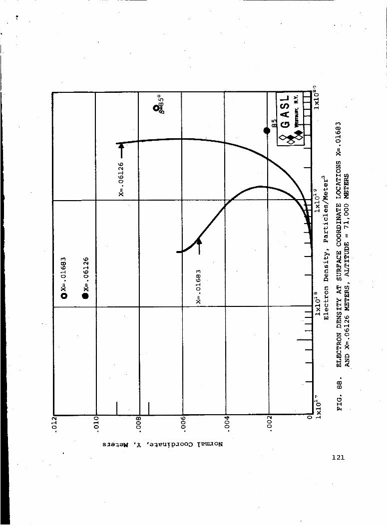
t
,-4O
(D%0,-4O
O
%Oc_
%0O
,-4%Oo
e
@
IO,-4o
sae_aN
I0o0o
o o oo o o
(D
o ,-4
'A 'e_eu_paooD IE_ON
121
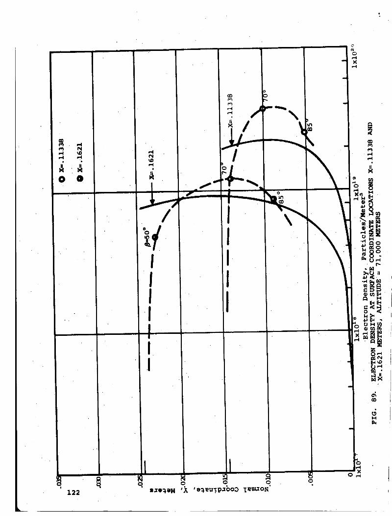
0
i 0
0
X
122
mmmmmmmm
0 0 0 0
a__0

r,-
,-i o o,-4 o
OO0
•Q u'_
'i', v l,, oII I _ _ OoOiI I
<.-7o_-r _ _,,
,I I o_.- _ _
I - _ _II I I _ _ _II I -, _ _
,,,II I _o ..
,I I -"_ii i -- _,
I I C_i _
"1 o1, - " _o°_I _ _ _
II T o
I I . '-
I! s0 _ 0 I.n 0,-'1t",i _iI ,-4 0
s_e_W 'A 'a_uTp_ooD I E[ua°N 123
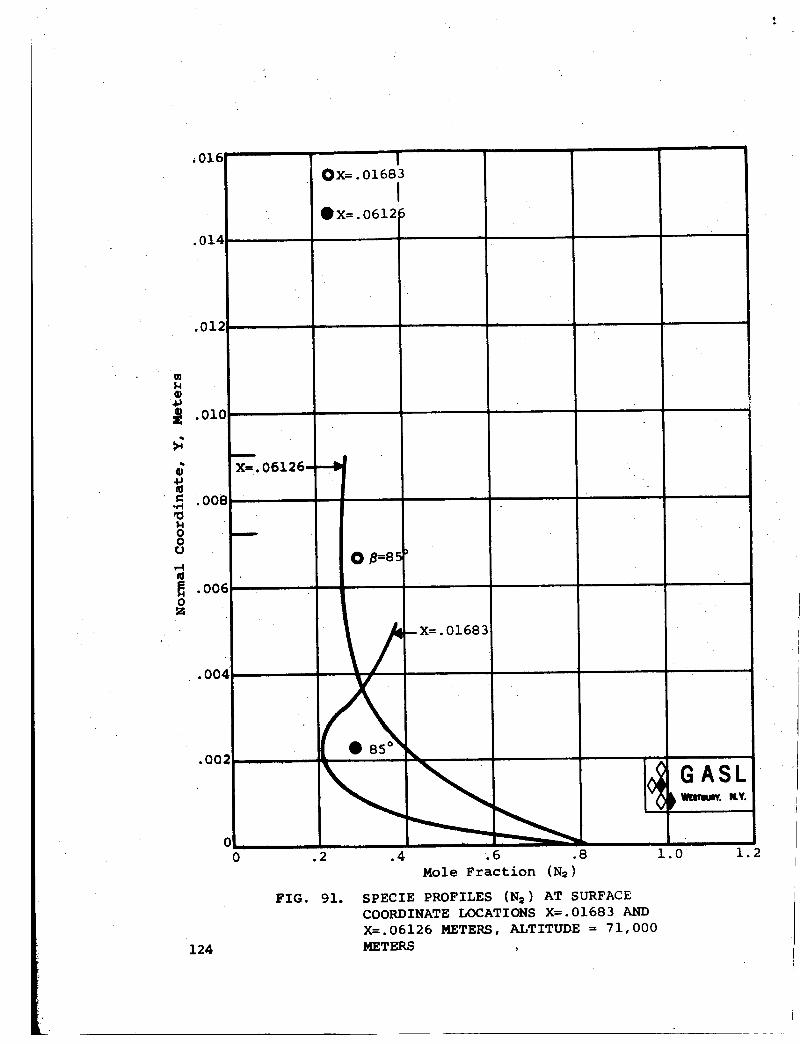
0
L
m
016
.014
.012
.010
.IJ
°_
oo
X_ • 06126-
IOX=. 01683
I
_X=.06121
0 B=85
i _/--X=.01683
.006 %
.004 _ ,, .
, \085°_
.oo= .... , G ASL
00 .2 .4 6 .8 1.0
Mole Fraction (N2)
FIG. 91. SPECIE PROFILES (N_) AT SURFACE
COORDINATE LOCATIONS X=.01683 AND
X=.06126 METERS, ALTITUDE = 71,000
METERS _124
1.2

00U
,-.I
.032
•028
.024
.020
IOX=.I1338
0X=.16211
/.016 /
__ W
Z/ o°_ p.o12
.008 _/85°
.004
/"/"
N H •
jJ
X=.1621
.3 .4 .5 .6 .7
Mole Fraction (N_)
FIG. 92. SPECIES PROFILES (N2) AT SURFACE
COORDINATE LOCATIONS X=.I1338 AND
X=.1621 METERS, ALTITUDE = 71,000 METERS
.8
125
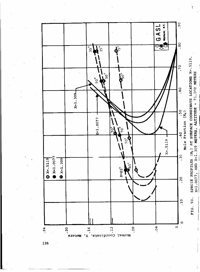
,-4 0 0_I 0I.CI °
,__O0 0
o
H
0
0
126


e,io
I
i
II
\
O
O
X_4
7o
Io
,-4M
o
u%04O
\\
I_1 _-I _ 00 0 0 0
/
o
c_
o_
,.q
I1"
_D
II"
H
O
ZH
OO
UI
mO
_O
O t"_
H £'4U H'_1 [-4
m<
t/3
H
s_a_ 'A 'a_Ru_pxooD IEU_ON128

0_.-4.,-4u',
IIX
0
o,-4
o,4
o_ ,-4
J
a
o
o
,-4IIX
Z0I-4E*
<ZI-4
"-" CJ
,-4
v
in
i-4
O
0.,
H
[.,.]a_
_n
oOO
r'-
tl
o_,-4
Oo
,.--4
_,Oo_
H
129

.01_
.o14
.012
.010
.OO2
00
130
• " m
O X=. 06126
0 X=. 0168
.06126
• 85 °
.1
11G. g7.
GASL
.2 .3 .4 .5
Mole Fraction (N)
SPECIE PROFILES (N) AT SURFACE COORDINATE
X_.06126 AND X-.01683 METERS,
ALTITUDE = 71,000 METERS
.6
i I ,
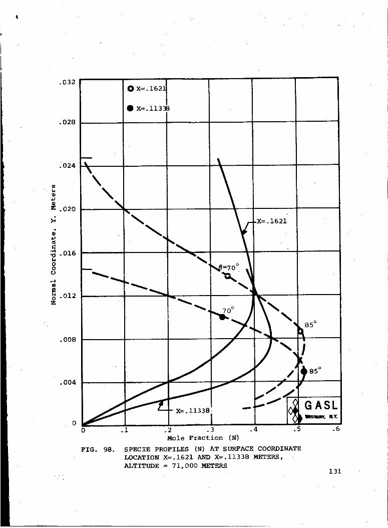
t
.032
.028
024
4_
=_ .020
4.1
" -r,I
.016
oou
,-4m
_ .012o
0 x=.162]
• x=.1133s
m
k , .
\\
"_"_ .x:.16_1
',,#:7o° _,!
.004 -- r
_ _'-t_ _x:.11338, -- G A SL0 _ wmmm¢. I1.%'.
0 .i .2 .3 .4 .5
Mole Fraction (N)
FIG. 98. SPECIE PROFILES (N) AT SURFACE COORDINATE
LOCATION X=. 1621 AND X=. 11338 METERS,
ALTITUDE = 71,000 METERS
.6
131

i._0'_ I_ 0_
0 0,-.I 0u_
0 00
132
o
o
s _'e_,es "A
oo u%u% 00GO
r,-
oG
,-4II
X
//
u% o
o
I!°II
'&_uTp=ooD _=o_
o o
0_
,-4i£'1
Co,-.4X
,--4
70,-4
0tIo
,-4
+o,.-4
,r
o
o,-IX
0
o •o
,.-.4
o+,-4ut_
IIX
Z0H
r_
i-4o
_o o
0.4 It,]II.o 0
mH
,-.4
_d
m_
H
O0
_ •
H
1'I

•018
•016
.014
.012
m
_.010
._ • 008
oou
_.006o
.004
.002
IO X=. 06126
IQ X=. 01683
I
X=.01683
X=.06126-
i
ii
0.18 .2O
FIG. i00.
.22 .24 .26 .28
Mole Fraction (O)
SPECIE PROFILE (0) AT SURFACE COORDINATE
LOCATION X=.06126 AND X=.01683 METERS,
ALTITUDE = 71,000 METERS
.30
133

.036
.032
.02E
OX=. 162]
OX=.I1338
l,
ii• ,m
w
.02G
d
c 016_J
0 __0
U
,--4
•012O
008,
•004
134
0_
.18 .20
FIG. 101.
X=. 1621 -- D
\
%
70 °
\\
, /85 °
-X=.I1338
I,
.22 .24 .26 .28
Mole Fraction (O)
SPECIE PROFILES (O) AT SURFACE COORDINATE
LOCATION X=.1621 AND X=. 11338 METERS,
ALTITUDE = 71,000 METERS
.30

.36
.32
.28
.24
®4J
(_=I. 007";
OK:. 5119
_:1.3o9
, ,,i
I
,I
.20
X=l. 0077-
_.16 .....
o== =,=,==. _=_
.12 i
.04 , =
_-X=. 5 i//_19
0
0 .05 .i0 .15 .20 .25 .30
Mole Fraction (O)
FIG. 102. SPECIE PROFILES (0) AT SURFACE
COORDINATE LOCATION X=I.0077, X=. 5119,
AND X=1.309 METERS, ALTITUDE = 71,000METERS 13-5

.018
.016
.014
012
.010
X
4.1
_ 008c °
8
,--4
, m . 006
o
.004
.002
136
_X=. 0168. _
_X=. 0612_
_X=. 11336
K=.I1338
- /.
/\
X=.06126
\\
\\
'Ii
//
/_" _ 85 °
70 °
J
--X=. 01682
0 .02 .04 .06 .08 .i0 .12
Mole Fraction (NO)
SPECIE PROFILES (NO) AT SURFACE COORDINATE
LOCATION X=.01683, X=.06126, AND X=.I1338
METERS, ALTITUDE = 71,000 METERS
FIG. I03.

.18
O x=.511s
• x=.1621
.16
.14
i
-- x=. 5119
.12 ,w
35 °
_.10 .
_ 08 '
' _ 06
o_ _
0 _ wa_u_,, N.y.
0 .02 .04 .06 .08 .i0 .12 .
Mole Fraction (NO)
FIG. 104. SPECIE PROFILES (NO) AT SURFACE COORDINATE
LOCATIONS X=.5119 AND X=.1621 METERS,
ALTITUDE = 71,000 METERS
137

.36
.32
.28
.24
.20
16
oou
_ .120
.08
• O4
0
138
5°
35 °
IO X=I. 0077
-X=I. 0077
i
!
• i _ X=I. 309
ill
)
[ ,!
0 .02
FIG. 105.
.04 .06• .08 .i0
Mole Fraction (NO)
SPECIE PROFILES (NO) AT SURFACE
COORDINATE LOCATION X=I.0077 AND
X=1.309 METERS, ALTITUDE = 71,000
METERS
•.12

,-Io
kD('_ a)
_D ,.-I0 0
IIx _0 Q
o
_0
.,.._
0
IIi
qr
I
0
u_{:9N
r_
GO_D
0
Yd
Io o 0o o o
sxe_eM 'A '_uTp_ooo I_U_ON
Io
1 _ ooo
_o_i
doo
139
"_'0
mc

%
.03_
.02E
r_
Z.020
4rd
._. 016
I.l00
,.-.4
_.012o
.O08
.004
140
O X=. 1621
OX=. i1338
t
B'=s
\.\
70 °
85 °
X=. 1621 _
X=. i1338
/ /
0 .0002
FIG. 107.
.0004 .0006 .0008 .0010
Mole Fraction (NO + ) and (e-)
SPECIE PROFILES (NO + ) AND (e-) AT SURFACE
COORDINATE LOCATION >[--.1621 AND >[--.11338
METERS, ALTITUDE = 71,000 METERS
.0012 .0014
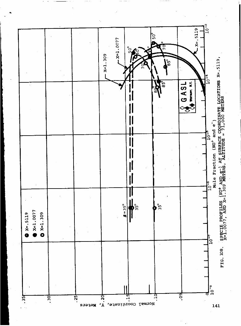
un
+
Oh _ O_r4 0 0
• _ _
OO0
I
141

, ° ° , ° ° ° • ° ° • . ° 0° °
0o
r_
_D
0m
%
B
o
0
0U
o.-.-I
M
_o
\
ooo
ou_
g• 0 0
'- o
_D
Go
,.4
o
,_ _ o co _ ,_. _ o _ _ _ _ o co _ ',_• • ° • • (_ 0• • • •
e_ _ r_ rn c_ c_ c_ c_ c_ _4 _ _ _ _ 0 0 0
142 NH/_ _ _ _q._.VNI(_HOOD q_WHON q_NOISN_41G-NON
Z
om
OO[J
o
O
o
c_
o
(13
,4
r,l
,-.i
o
o
d
c;
o
o

0
G
i'oo
II
rj
o
ooo
oooo
oooo
%oo
oooo
o
d
• , • • • ° o• °
N_/_ _ _I_M000 T4W_ON T4NOIS"N_I_-f_ON143

• , l • l , . _ _ : . , .
co
00
_o
Nun
o
_D
,.D
I-
X
oN
oU
0U
,-4,-4,...I
_ 0
N
Nt_
o
%
,-.4 _,
%
L_
• • . . • . o • •
N_/_ _.T._I(I_OOD '_P_O_ _OIS_3?_I(I-_O_
144
_o
o
co
_D
,So
co[.-i
00
4 _
4 _
r.,
_ o
o0
t_
_4
d
d
c,l
o
(13
,-4
tip
,-4
e-t
,-.-i
o
,.-4
0g
o
o
o
o
o

J
oo
0z
1.6
1.4
1.2
1.0
.8
.6
.4
00
X=I.0077, X=1.309
X=.5119
/
X=.1621 [
GASL
f" _i 338
X =.06126
I Ix='°_i000 2000 3000 4000 5000
Pressure, Newtons/Meter e
FIG. 112_ PRESSURE PROFILES AT SURFACE COORDINATE
LOCATIONS X=.01683, X=.06126, X=.11338,
X=.1621, X=.5119, X=I.0077, AND X=1.309
METERS, ALTITUDE = 71,000 METERS145