n w it h n o r m c o s t f u n c t io n scvgmt.sns.it/media/doc/paper/1303/sel.partmonge.pdf · a p...
TRANSCRIPT

AN EXISTENCE RESULT FOR THE MONGE PROBLEM IN n
WITH NORM COST FUNCTIONS
LAURA CARAVENNA
Abstract. We establish existence of solutions to the Monge problem in n with a norm cost function,assuming absolute continuity of the initial measure.
The loss in strict convexity of the unit ball implies that transport is possible along several directions.As in [4], we single out particular solutions to the Kantorovich relaxation with a secondary variationalproblem, which involves a strictly convex norm. We then define a map rearranging the mass within therays, by a Sudakov-type argument with the disintegration technique in [8, 10, 17].
In the secondary variational problem the cost is also infinite valued and in general there is no Kan-torovich potential. However, all the optimal transport plans share the same maximal transport rays.We derive also an expression for the transport density associated to these optimal plans.Remark: The construction presently given in the preprint needs the further technical assumption that,with the notation of Section 3.4, the set of points x ! Ts whose secondary transport ray belongs to therelative border of the convex envelope of {y : !(x) " !(y) = #y " x#} is µ-negligible.
Contents
1. Introduction 11.1. An account on the literature 21.2. Overview of the paper 42. The Secondary Transport Problem 72.1. A universal family of secondary transport rays 82.2. Statement of the disintegration w.r.t. secondary transport rays 112.3. Solutions to the Monge secondary transport problem 122.4. Determination of the transport density 153. The Disintegration w.r.t. Secondary Transport Rays 183.1. Partition of the secondary transport set into model sets 213.2. Negligibility of border points 223.3. Partition of the primary transport set into invariant sets 243.4. Construction of a local secondary potential 253.5. Approximation lemma and disintegration 284. Notations 31References 32
1. Introduction
Topic of this paper is the existence of solutions to the Monge problem in n when the cost function isgiven by a norm !·!, possibly asymmetric: given two Borel probability measures µ, ! " P( n), we studythe minimization of the functional
IM (t) =
!
n
!t(x)# x! dµ(x) (MP1)
Date: September 10, 2009.Key words and phrases. Monge problem, deterministic transference plans, disintegration of the Lebesgue measure,
transport rays, absolute continuity of the conditional measures, norm cost function, transport density, Kantorovich potential,Sudakov theoremMSC: 49J20 (49K40 49Q20), 28A50.
1
AN EXISTENCE RESULT FOR THE MONGE PROBLEM IN n WITH NORM COST FUNCTIONS 2
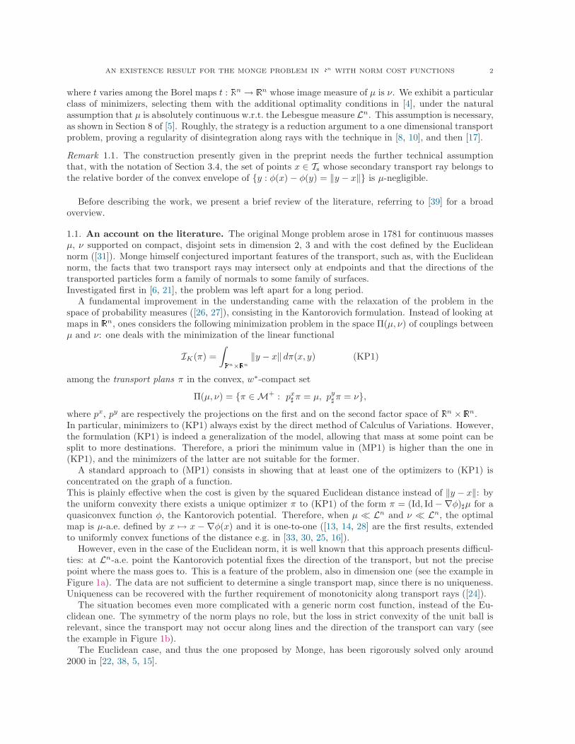
where t varies among the Borel maps t : n $ n whose image measure of µ is !. We exhibit a particularclass of minimizers, selecting them with the additional optimality conditions in [4], under the naturalassumption that µ is absolutely continuous w.r.t. the Lebesgue measure Ln. This assumption is necessary,as shown in Section 8 of [5]. Roughly, the strategy is a reduction argument to a one dimensional transportproblem, proving a regularity of disintegration along rays with the technique in [8, 10], and then [17].
Remark 1.1. The construction presently given in the preprint needs the further technical assumptionthat, with the notation of Section 3.4, the set of points x " Ts whose secondary transport ray belongs tothe relative border of the convex envelope of {y : "(x) # "(y) = !y # x!} is µ-negligible.
Before describing the work, we present a brief review of the literature, referring to [39] for a broadoverview.
1.1. An account on the literature. The original Monge problem arose in 1781 for continuous massesµ, ! supported on compact, disjoint sets in dimension 2, 3 and with the cost defined by the Euclideannorm ([31]). Monge himself conjectured important features of the transport, such as, with the Euclideannorm, the facts that two transport rays may intersect only at endpoints and that the directions of thetransported particles form a family of normals to some family of surfaces.Investigated first in [6, 21], the problem was left apart for a long period.
A fundamental improvement in the understanding came with the relaxation of the problem in thespace of probability measures ([26, 27]), consisting in the Kantorovich formulation. Instead of looking atmaps in n, ones considers the following minimization problem in the space !(µ, !) of couplings betweenµ and !: one deals with the minimization of the linear functional
IK(#) =
!
n! n
!y # x! d#(x, y) (KP1)
among the transport plans # in the convex, w"-compact set
!(µ, !) = {# "M+ : px! # = µ, py
!# = !},
where px, py are respectively the projections on the first and on the second factor space of n % n.In particular, minimizers to (KP1) always exist by the direct method of Calculus of Variations. However,the formulation (KP1) is indeed a generalization of the model, allowing that mass at some point can besplit to more destinations. Therefore, a priori the minimum value in (MP1) is higher than the one in(KP1), and the minimizers of the latter are not suitable for the former.
A standard approach to (MP1) consists in showing that at least one of the optimizers to (KP1) isconcentrated on the graph of a function.This is plainly e"ective when the cost is given by the squared Euclidean distance instead of !y # x!: bythe uniform convexity there exists a unique optimizer # to (KP1) of the form # = (Id, Id#&")!µ for aquasiconvex function ", the Kantorovich potential. Therefore, when µ ' Ln and ! ' Ln, the optimalmap is µ-a.e. defined by x ($ x #&"(x) and it is one-to-one ([13, 14, 28] are the first results, extendedto uniformly convex functions of the distance e.g. in [33, 30, 25, 16]).
However, even in the case of the Euclidean norm, it is well known that this approach presents di#cul-ties: at Ln-a.e. point the Kantorovich potential fixes the direction of the transport, but not the precisepoint where the mass goes to. This is a feature of the problem, also in dimension one (see the example inFigure 1a). The data are not su#cient to determine a single transport map, since there is no uniqueness.Uniqueness can be recovered with the further requirement of monotonicity along transport rays ([24]).
The situation becomes even more complicated with a generic norm cost function, instead of the Eu-clidean one. The symmetry of the norm plays no role, but the loss in strict convexity of the unit ball isrelevant, since the transport may not occur along lines and the direction of the transport can vary (seethe example in Figure 1b).
The Euclidean case, and thus the one proposed by Monge, has been rigorously solved only around2000 in [22, 38, 5, 15].

AN EXISTENCE RESULT FOR THE MONGE PROBLEM IN n WITH NORM COST FUNCTIONS 3
t1
t2
I1
I2
I2
I3
(a) One dimensional example. Let µ be the Lebesguemeasure on I1 $ I2 % and " the Lebesgue measure onI2 $ I3. Both the maps t1 translating I1 to I2, I2 toI3 and the map t2 translating I1 to I3 and leaving I2fixed are optimal. Moreover, any convex combinationof the two transport plans induced by t1, t2 is again aminimizer for (KP1), but clearly it is not induced by amap.
{!x! ) 1}
Q1 Q2
Q3
Q0
t1
t2
(b) Two dimensional example. The unit ball of #·# isgiven by the rhombus. Let µ be the Lebesgue measureQ0 $Q1 % 2 and " the Lebesgue measure on Q2 $Q3.Both the maps t1, t2 translating one of the first twosquares to one of the second to squares are optimal, andthey transport mass in di!erent directions.
Figure 1: Examples of non uniqueness of optimal transport maps with a generic norm.
Roughly, the approaches in the last three papers is at least partially based on a decomposition of thedomain into one dimensional invariant regions for the transport, called transport rays. Due to the strictconvexity of the unit ball, these regions are 1-dimensional convex sets. Due to regularity assumptions onthe unit ball and a clever countable partition of the ambient space, it is moreover possible to reduce tothe case where the directions of these segments is Lipschitz continuous. This, by Area or Coarea formula,allows to disintegrate the Lebesgue measure w.r.t. the partition in transport rays, obtaining absolutelycontinuous conditional probabilities on the one dimensional rays. In turn, this su#ces to perform areduction argument, that we also use in the present paper, which yields the thesis: indeed, one canfix within each ray an optimal transport map, uniquely defined imposing monotonicity within each ray.However, as in [10, 17, 18], we do not rely on any Lipschitz regularity of the vector field of directions.This kind of approach was introduced already in 1976 by Sudakov ([37]), in the more generality of apossibly asymmetric norm — which actually is the case we are considering. However, its argument remainsincomplete: a regularity property of the disintegration of the Lebesgue measure w.r.t. decompositions ofthe space into a#ne regions was not proved correctly, and, actually, stated in a form which does not hold([2]). Indeed, there exists a compact subset of the unit square having measure 1 and made of disjointsegments, with Borel direction, such that the disintegration of the Lebesgue measure w.r.t. the partitionin segments has atomic conditional measures ([29, 1]). The reduction argument described above requiresinstead absolutely continuous conditional measures, in order to solve then the one dimensional transportproblems, and therefore a regularity of the partition in transport rays must be proved.In the case of a strictly convex norm, where the a#ne regions reduce to lines, Sudakov argument wascompleted in [17]. In this paper we choose an alternative one dimensional decomposition selected by theadditional variational principles, instead of the a#ne one considered by Sudakov.

AN EXISTENCE RESULT FOR THE MONGE PROBLEM IN n WITH NORM COST FUNCTIONS 4
The method in [22] is based on PDEs and they introduce the concept of transport density, widelystudied since there — the very first works are [23, 2, 12, 24], in [34] one finds more references. Givena Kantorovich potential u for the transport problem between two absolutely continuous measures withcompactly supported and smooth densities f+, f#, they define as transport density a nonnegative functiona supported on the family of transport rays and satisfying
# div(a&u) = f+ # f#
in distributional sense. The above equation was present already in [7] with di"erent motivation. It allowsa generalization to measures, and an alternative definition introduced first in [11] for $ := aLn is givenby the Radon measure defined on A " B( n) as
(1.1) $(A) :=
!
n! n
H1 (A * !x, y") d#(x, y),
where # is an optimal transport plan.When the unit ball in not strictly convex, the results available are in the two-dimensional case, which
is completely solved, and for crystalline norms ([4]). The strategy is to fix both the direction of thetransport and the transport map by imposing additional optimality conditions, and then to carry out aSudakov-type argument on the selected transports.
We follow the same strategy, and the disintegration technique available from [10], whose adaptationhowever is not really straightforward, allows to find the result for a generic norm.
A di"erent proof of existence for general norms, which does not rely on disintegration of measuresand is more concerned with the regularity of the transport density, is contemporary presented in [20],improving their argument for strictly convex norms in [19].
1.2. Overview of the paper. We present below an overview of the paper, where we establish existenceof minimizers to the Monge problem in n with a norm cost function. We follow the selection argumentin [4] in order to perform a one dimensional Sudakov-type decomposition of the space. We deal withthe key di#culty of disintegrating the Lebesgue measure w.r.t. this decomposition, arising because of themore general norm, following the technique introduced in [8, 10] and then in [17] for this setting.
We state the problems and introduce some notations before summarizing the results.
Primary Transport Problem. Consider the Monge-Kantorovich optimal transport problem
(1.2) min"$!(µ,#)
IK(#),
where
IK(#) :=
!
!y # x! d#(x, y)
between two positive Radon measures µ, ! with the same total variation. We assume that µ ' Ln and,in order to avoid triviality, we suppose moreover that there exists a transport plan with finite cost.
Let the optimal primary transport plans be the family Op + !(µ, !) of minimizers to the primaryproblem. Let moreover " be a Kantorovich potential, which is a function n $ such that
"(x) # "(y) ) !y # x! ,(x, y) " n % n(1.3a)
"(x) # "(y) = !y # x! for #-a.e. (x, y) ,# " Op.(1.3b)
Define $p as the !·!-subdi"erential of ", which is the set %#" = {(x, y) : "(x) # "(y) = !y # x!}.
Secondary Transport Problem. Consider a strictly convex norm | · |. Study
(1.4) min"$Op
!
|y # x| d#(x, y) = min"$!(µ,#)
IsK
where
IsK(#) :=
!
cs(x, y) d#(x, y)

AN EXISTENCE RESULT FOR THE MONGE PROBLEM IN n WITH NORM COST FUNCTIONS 5
and where the secondary cost function cs is defined by
cs(x, y) := |y # x| "p(x, y).
Let the optimal secondary transport plans be the family Os + !(µ, !) of minimizers to (1.4).
We establish the following theorem concerning the existence of optimal transport maps for the sec-ondary transport problem, and thus for the primary one. The proof will be given in Section 2.
Theorem. The following statements concerning the primary and secondary transport problems hold.1: Monge Problem.
There exists a unique optimal secondary transport plan #s " Os induced by a map t monotone along rays.More precisely, it is induced by a Borel map t such that
- for all x " n the outgoing ray r+(x) := -n$ !x, tn(x)" is a segment;- for all x " n the map t !r+(x) is monotone;- the graph of t is &-compact.
Then, the graph of r+, of the secondary transport rays r := r+-(r+)#1 and of the vector field d vanishingwhere t(x) = x and pointing otherwise towards t(x)# x are &-compact.The optimal map t provides a solution to the primary Monge problem which may change with | · |.
2. Secondary Transport Problem.Every optimal secondary transport plan #s " Os is concentrated on the cs-monotone set Graph(r+).In particular, there exists a &-compact subset Q of countably many hyperplanes such that the family ofnon trivial oriented segments defined by {rq := r (q)}q$Q has the following properties:
- t(x) .= x for all x in Ts := -q$Qrq which is not a terminal point of some rq;- t(x) = x for all x in F = n \ Ts;- (µ + !)-a.e. fixed points of t are fixed points for every #s " Os;- for Hn#1-a.e. q " Q, rq is an invariant sets for every #s " Os.
3. Secondary Transport Density.The transport density (1.1) associated to any optimal secondary transport plan #s " Os is the uniquesolution $ = aLn, a " L1
loc(n), to the transport equations, for Z " B(Q) arbitrary open sets,
div( r (Z)d $) = r (Z)(µ# !) $ "M+loc
whose density vanishes moving on the rays towards initial points, and out of Ts. It may vary with | · |.
We give in (2.12) two formulas for the transport density, in terms of either the disintegrations of µand ! or the map t, following Section 8 of [10]. It satisfies a divergence formula on ‘regular’ subsets ofr (Z), for Z " B(Q).
The above theorem is derived as a corollary of the regularity of the disintegration w.r.t. transport rays,stated below, and of the dimensional reduction arguments present in the literature.
The basic idea is the following. If we had two regions invariant for the transport, and it were possibleto define an optimal transport map for the restricted measures within each region, then we would triviallyget an optimal transport map solving our problem.The same reasoning is applied to the continuous family of invariant sets {rq}q$Q by means of the dis-integration theorem. In order to solve the transport problem on each segment, one needs the absolutecontinuity of the initial measure to be transported on the segment. If that holds, the one dimensionalsolution is know and one shows that the maps on each segment provide together an optimal transportplan.
The issue of the following disintegration theorem is indeed to show that disintegrating the Lebesguemeasure on the secondary transport set Ts = -q$Qrq one obtains conditional measures absolutely contin-uous w.r.t. the Lebesgue measure on the segments.
We state here below the Disintegration Theorem by itself, starting from a cs-monotone set $ anddefining the transport rays related to $. In view of the application to the transport problem, we directlyassume w.l.o.g. $ &-compact and contained in {cs < +/}. Indeed, one obtains the statement of the

AN EXISTENCE RESULT FOR THE MONGE PROBLEM IN n WITH NORM COST FUNCTIONS 6
theorem above choosing $s as the graph of the multivalued function x $ r+" (x) in Definition 2.2, whenever$ is chosen as a cs-monotone, &-compact carriage for any optimal secondary transport plan # " Os
contained in {cs < +/}.The following construction of the transport rays is similar to the one in [4], and it is present in
several other papers in terms of the Kantorovich potential of the transport problem. The definition ofdisintegration is recalled in Definition 2.10, while the one of cs-monotone set in Definition 2.1.
Definition 1.2. Given a set $ + n % n, define the multivalued map r : n $ n having graph"
(x, y) : 0(x%, y%) " $s such that !x, y" 1 !x%, y%"
#
.
and the following equivalence relation in Graph(r ):
(x, w)s2(y, z) 34 r (x) * r (w) = r (y) * r (z).
The possible r.h.s. identify the equivalence classes, denote the family of those ones which are not singletonsas the family {rq}q$Q of transport rays relative to $.The relative transport set is the union of the transport rays: Ts = -q$Qrq.Define d as the multivalued vector field giving at each point x " Ts the unit direction from x to any pointin r (x), and vanishing elsewhere.
Theorem. Let $ be a &-compact, cs-monotone subset of {cs < +/}. Define the relative &-compacttransport set Ts and its covering by secondary transport rays {rq}q$Q and d as in Definition 1.2.
Then, the following strongly consistent disintegration w.r.t. the covering {rq}q$Q holds:
(1.5) Ln Ts =
!
Q
$
' H1rq
%
dHn#1(q)
where ' : n $ + \ 0 is a Borel function and Q is a &-compact subset of countably many hyperplanes.In particular, the set of endpoints E of the secondary transport rays {rq}q$Q is Ln-negligible and there-
fore {rq}q$Q is a partition of Ts, removing an Ln-negligible set.Moreover, a Green-Gauss-type divergence formula holds on special subsets of the transport set for the
vector field of secondary rays directions d .
The proof of the theorem will be given in Section 3, following [8, 10, 17].A di#culty consists in the fact that in this approach the disintegration technique naturally involves aHopf-Lax formula with a Kantorovich potential for the secondary transport problem, in order to definea more regular vector field of directions approximating the directions of the secondary transport rays —for which in our case no regularity is known more than Borel measurability.However, since cs is /-valued and only lower semicontinuous, in general there is no function "s such that$s is the cs-subdi"erential of "s, which would correspond to a Kantorovich potential for the secondarytransport problem — see Example 3.14.
The disintegration strategy consists basically in the following. One reduces the Lebesgue measure tospecial sets made of secondary rays transversal to an hyperplane H0, by a countable partition. Let Ht
denote an hyperplane at distance t from H0, on the side where terminal points of secondary rays lye ift > 0, on the other otherwise. The special sets Z have to be chosen so that the following approximationholds: if we consider the subset Z % of those secondary rays intersecting an hyperplane Ht, the restrictionof d to Z %*Ht is Hn#1-a.e. the pointwise limit of a sequence of vector fields each pointing towards finitelymany points of a dense sequence in Z % * Hs, for any Hs di"erent from Ht which is transversal to therays in Z % (see Figure 2). This approximation by cones provides quantitative estimates of the Hausdor"(n#1)-dimensional measure of the intersection Z *Ht between the hyperplane Ht parallel to H0 and thesecondary rays of Z. The transversality of the hyperplanes ensures that the membership to a secondarytransport ray establishes a bijective correspondence between the points of these parallel sections. Theestimates on the Hausdor" measure of Z *Ht yields that the Hn#1-measure on each section is absolutelycontinuous w.r.t. the push forward measure, by the map above defined by the membership to a same

AN EXISTENCE RESULT FOR THE MONGE PROBLEM IN n WITH NORM COST FUNCTIONS 7
Figure 2: Cone approximation.
secondary transport ray, of the Hausdor" measure on a fixed intermediate section, say Z0 := Z * H0.This leads to a justification of the following steps, with the notation of measure disintegrations
Ln(x) Z =
!
(Hn#1(x) Zt) dt by Fubini-Tonelli, where Zt = Z *Ht
x$Zt&q$Z0=
!"
((t, q)Hn#1(q) Z0
#
dt by the push forward estimates on the sections
=
!
Z0
(((t, q)H1(t)) dHn#1(q) by Fubini-Tonelli, since ( is regular enough
x=q+td (x)=
!
Z0
('(x)H1(x) rq) dHn#1(q).
The new part of the construction, in Section 3, amounts thus in exhibiting a countable partition of thesecondary transport set into model sets where one can prove the estimate on the push forward measure.
We first provide a secondary potential "s for a suitable restriction of the plan. Then, looking e.g. atthe sections Z0, Zt, we choose the following approximating vector field of directions restricted to Zt: thevector field defined by the correspondence
y ($ argminx$Z0
&
"(x) + )"s(x)'
+&
!y # x! + )|y # x|'
.
It substitutes the cone approximation described above, due to the fact that it is almost a potential w.r.t. astrictly convex norm and therefore it can in turn be approximated by cone functions.The secondary potential is exhibited on subsets of Ts such that, when partitioned into invariant sets forthe primary transport problem, any two points can be connected by a coordinate cycle with finite cost,we will be more precise in Subsection 3.4.
The second e"ort is in order to provide a countable partition of Ts which reduces the disintegrationproblem to the model sets, and which is based on a partition of T into invariant sets for the primaryproblem — useful for the construction of the ‘local’ secondary potential "s. We partition first a subsetof Ts, and we show then that the set left apart with the partition has zero Lebesgue measure.
2. The Secondary Transport Problem
The secondary transport problem is a Monge-Kantorovich problem
min"$!(µ,#)
!
cs(x, y) d#(x, y)
AN EXISTENCE RESULT FOR THE MONGE PROBLEM IN n WITH NORM COST FUNCTIONS 8
w.r.t. the secondary function
cs(x, y) = |y # x|*{(x,y): $(x)#$(y)=|y#x|}(x, y).
This problem on one hand is more di#cult than the primary one, since the secondary cost function isnot continuous and takes the value +/. The advantage is that the strict convexity on regions which areinvariant sets for the primary problem implies the known fact that any secondary optimal transport planmoves mass along rays.
We remind the following definition.
Definition 2.1. Given a cost function c : n % n $ +, a subset $ of n % n is c-monotone if for allfinite number of points {(xi, yi)}i=1,...,M belonging to $ one has the following inequality:
c(x0, y0) + · · · + c(xM , yM ) ) c(x0, y1) + · · · + c(xM#1, yM ) + c(xM , y0).
Any optimal plan # for a Monge-Kantorovich problem in Polish spaces with a positive, analytic costfunction c, and such that
(
c d# < /, is concentrated on a c-monotone set (Lemma 5.2 in [9]). Whenthe cost c is continuous, one is moreover allowed to take as this set the support of #. As a consequence,there exists a closed set $ + {c < +/} such that every optimal transport plan is supported on $: forany dense sequence {#k}k$ in the convex, w"-closed set of optimal transport plans and one can take as$ the support of the secondary optimal transport plan
)
k$ #k/2#k.This is no more true when the cost function is not continuous and possibly +/-valued, since the
closure of a c-monotone set in general is not c-monotone. However, all the secondary optimal transportplans for cs are concentrated on a common cs-monotone set, and therefore they share the same transportrays (Lemma 2.11).
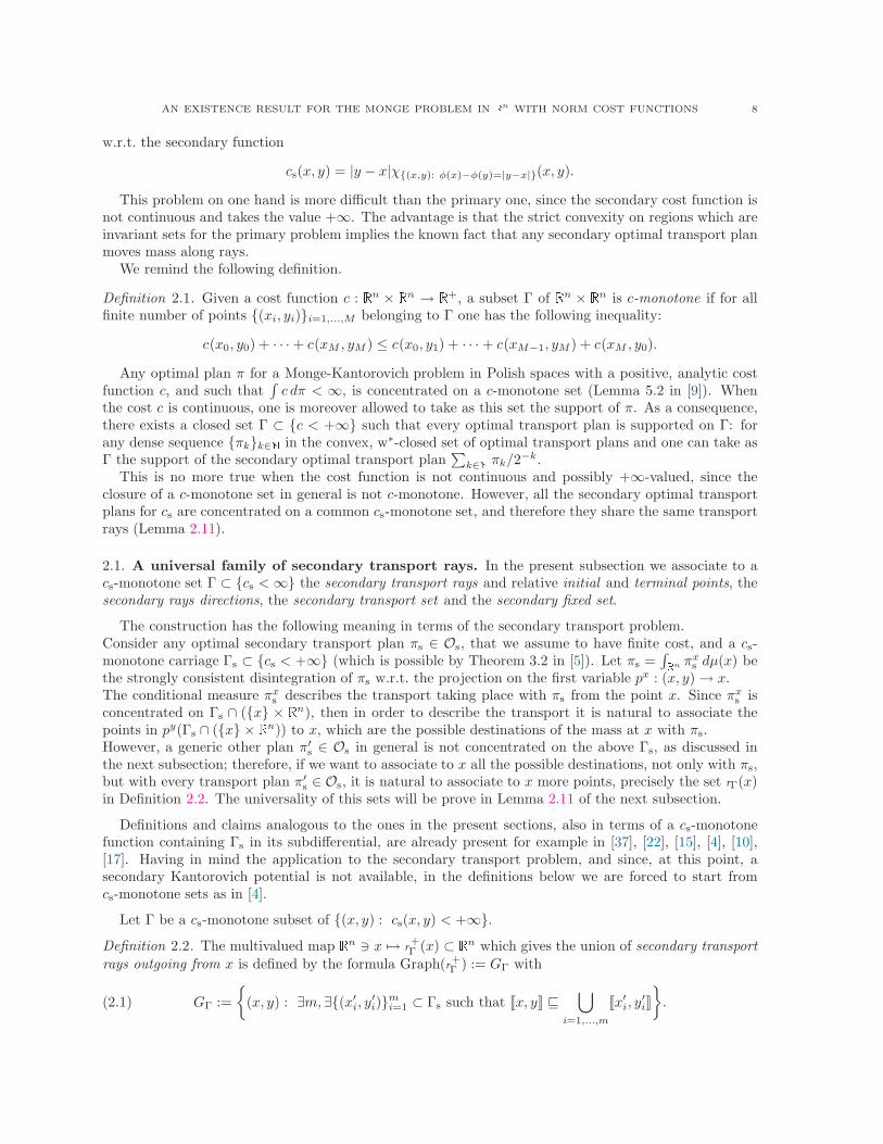
2.1. A universal family of secondary transport rays. In the present subsection we associate to acs-monotone set $ + {cs < /} the secondary transport rays and relative initial and terminal points, thesecondary rays directions, the secondary transport set and the secondary fixed set.
The construction has the following meaning in terms of the secondary transport problem.Consider any optimal secondary transport plan #s " Os, that we assume to have finite cost, and a cs-monotone carriage $s + {cs < +/} (which is possible by Theorem 3.2 in [5]). Let #s =
(
n #xs dµ(x) be
the strongly consistent disintegration of #s w.r.t. the projection on the first variable px : (x, y) $ x.The conditional measure #x
s describes the transport taking place with #s from the point x. Since #xs is
concentrated on $s * ({x} % n), then in order to describe the transport it is natural to associate thepoints in py($s * ({x} % n)) to x, which are the possible destinations of the mass at x with #s.However, a generic other plan #%
s " Os in general is not concentrated on the above $s, as discussed inthe next subsection; therefore, if we want to associate to x all the possible destinations, not only with #s,but with every transport plan #%
s " Os, it is natural to associate to x more points, precisely the set r"(x)in Definition 2.2. The universality of this sets will be prove in Lemma 2.11 of the next subsection.
Definitions and claims analogous to the ones in the present sections, also in terms of a cs-monotonefunction containing $s in its subdi"erential, are already present for example in [37], [22], [15], [4], [10],[17]. Having in mind the application to the secondary transport problem, and since, at this point, asecondary Kantorovich potential is not available, in the definitions below we are forced to start fromcs-monotone sets as in [4].
Let $ be a cs-monotone subset of {(x, y) : cs(x, y) < +/}.
Definition 2.2. The multivalued map n 5 x ($ r+" (x) + n which gives the union of secondary transport
rays outgoing from x is defined by the formula Graph(r+" ) := G" with
(2.1) G" :=
"
(x, y) : 0m, 0{(x%i, y
%i)}m
i=1 + $s such that !x, y" 6*
i=1,...,m
!x%i, y
%i"
#
.

AN EXISTENCE RESULT FOR THE MONGE PROBLEM IN n WITH NORM COST FUNCTIONS 9
The map r giving the secondary transport rays through x identified by the formula Graph(r ) = G"-(G")T ,where (G")T is the transpose of G".When specifying otherwise which is a set $ defining G", we will denote r" simply as r .
Remark 2.3. As quickly discussed above, the ones of Definition 2.2 should be called more properly themaximal secondary transport rays associated to $, while the secondary transport rays r %+" , r %" associatedto $ should be similarly defined from
(2.2) G%" :=
"
(x, y) : 0(x%, y%) " $s such that !x, y" 6 !x%, y%"
#
.
Since we are mainly interested in the maximal secondary transport rays, we put them in evidence andwe define the ones from (2.2) as the $-secondary transport rays.Notice that r+" (x) = -i$ (r %+)i(x), which is the set -i$ Ki with K0 := {x} and Ki := -r %+" (Ki#1).
Definition 2.4. We define the following equivalence relation in Graph(r ) (see Lemma 2.9 below):
(2.3) (x, w)s2(y, z) 34 r (x) * r (w) = r (y) * r (z).
The r.h.s. of (2.3) identifies the equivalence classes.Secondary transport rays . A (nontrivial) secondary transport rays is each element in the r.h.s. abovewhich do not reduce to a single point. We denote the family of secondary rays with {rq}Q.Endpoints . The endpoints of a ray rq are the points in its relative border. Let E be the set of endpointsof secondary transport rays.Initial and terminal points . The terminal and initial points of a ray rq are, when they exist, those a, b " rqsuch that, respectively, r+(b) = {b} and (r+)#1(a) = {a}. Denote with E# the set of initial points andwith E+ the set of terminal points of secondary transport rays.Secondary transport set . The secondary transport set is the union of secondary transport rays:
Ts =*
q$Q
rq = px(Graph(r")).
Fixed set . The fixed set is the complementary of the transport set.Rays direction. The direction of a ray rq is the unit vector pointing from the initial to the terminal pointof rq. The multivalued vector field d : n $ Sn#1 of rays directions gives at each point x " Ts thedirection of the rays through x and vanishes elsewhere.
Remark 2.5. The equivalence classes of (2.3) which do not reduce to point are of the form
rq % rq = (rq % n) *Graph(r ),
where one should remove the two points {(e, e)} for initial or terminal points e of rq which belong alsoto other secondary transport rays. Therefore, the partition induced on ((Ts \ E) % n) *Graph(r !Ts
) isprecisely
+
(rq % n) *Graph(r ),
q$Q.
Remark 2.6. Suppose $ is compact. Then also the set in (2.2) must be compact: indeed, for everysequence (xk, yk) " Graph(r %"), (x%
k, y%k) " $ with !xk, yk" 1 !x%
k, y%k", by compactness of $ up to subse-
quences {(x%k, y%
k)}k$ converges to some point (x%, y%) " $; therefore, {(xk, yk)}k$ must converge, up tosubsequences, to a point (x, y): !x, y" 1 !x%, y%", thus belonging to Graph(r %").In particular, the set in (2.1) must be &-compact, by Remark 2.3.
Clearly, a &-compact $ defines then &-compacts G", G%".
As a consequence, when $ is &-compact the multivalued functions r , d and the function associatingto each point in Ts the initial and terminal points of the relative secondary transport rays, in the com-pactification of n with points at /, are Borel. As well, the secondary transport set, the set of initialpoints the set of terminal points are Borel. For detailed proofs see Lemma 2.2, Lemma 2.9 in [17] (takenfrom [10]).In particular, in this case also the projection map q : Ts $ Q has a &-compact graph, by the explicit

AN EXISTENCE RESULT FOR THE MONGE PROBLEM IN n WITH NORM COST FUNCTIONS 10
construction that we will give of the quotient space, intersecting branches of rays with a transversalhyperplane.
Lemma 2.7. Let (x, y) be such that cs(x, y) < /. Then cs(x%, y%) < / for all !x%, y%" ! !x, y".Moreover, if (z, w) is such that cs(z, w) < / and !x, y"* !z, w" .= 7, then cs(x%, y%) < / for all !x%, y%" !
!x, y" - !z, w".
Proof. This is an immediate consequence of the inequality "(x) # "(y) ) !y # x! for all (x, y):
"(x) # "(x%) + "(x%)# "(y%) + "(y%)# "(y) = "(x)# "(y) = !x% # x!+ !y% # x%!+ !y # y%!
implies "(x) # "(x%) = !x% # x!, "(x%)# "(y%) = !y% # x%!, "(y%)# "(y) = !y # y%!.The second claim is instead a consequence of the convexity of the norm: if x% " !x, y" - !z, w"
"(x) # "(w) = "(x) # "(x%) + "(x%)# "(w) = !x% # x! + !w # x%! ) !w # x!,
and therefore, since the opposite inequality holds for all (x, w), equality yields cs(x, w) < /. Since!x, y" - !z, w" is or !x, y", or !z, w", or !x, w", the first claim proves the second one. "
Lemma 2.8. For any two points (x%, y%), (x%%, y%%) " $ and any x such that !x%, y%"* !x%%, y%%" 5 x, then orx = x% = x%% or x = y% = y%% or the two segments !x%, y%", !x%%, y%%" are aligned.
Proof. Consider any x and any two points (x%, y%), (x%%, y%%) " $ such that !x%, y%"* !x%%, y%%" 5 x. Then wehave
(2.4) |y% # x%| + |y%% # x%%| = |y% # x| + |x# x%| + |y%% # x| + |x# x%%|.
On the other hand, the cs-monotonicity inequality
|y% # x%| + |y%% # x%%| = cs(x%, y%) + cs(x
%%, y%%) ) cs(x%%, y%) + cs(x
%, y%%)
together with the strict convexity inequalities
cs(x%%, y%) ) cs(x
%%, x) + cs(x, y%) = |x# x%%| + |y% # x|cs(x
%, y%%) ) cs(x%, x) + cs(x, y%%) = |x# x%| + |y%% # x|
(2.5)
implies
(2.6) cs(x%, y%) + cs(x
%%, y%%) ) cs(x%%, x) + cs(x, y%) + cs(x
%, x) + cs(x, y%%).
Since equality must old by (2.4), equality must hold also in (2.5): by the strict convexity of | · | definingcs, if the segments #x%, y%$ and #x%%, y%%$ are not parallel then either x = x% = x%% or x = y% = y%%. "
Lemma 2.9. Let $ be a cs-monotone subset of {cs < /}.Then, the set Graph(r+) is a cs-monotone subset of {cs < /} and (2.3) is a partition of it.Each set r (x) is either a segment or a union of segments having x as a common either initial, or terminalpoint.
Proof. We separate the three claims in the statement.
Claim 1: Finite cost . By the first claim in Lemma 2.7, cs(x, y) < +/ for all (x, y) " Graph(r %) in (2.2).Moreover, since r+(x) = -i$ (r %+)i(x), the second claim in Lemma 2.7 proves that also Graph(r+) iscontained in cs < /Claim 2: Cyclical monotonicity. Consider any M points {(x%
i, y%i)}i " Graph(r %+) in order to test the
definition of cs-monotonicity. Let {(x%i, y
%i)}i be points of $ such that #xi, yi$ 6 #x%
i, y%i$. Then, since $ is
cs-monotone-
|y%i # x%
i| )-
cs(x%i+1, y
%i),
where x%M+1 = x%
1, and we set also xM+1 = x1. The triangular inequality yields
cs(x%i+1, y
%i) ) |y%
i # yi| + cs(xi+1, yi) + |xi+1 # x%i+1|.

AN EXISTENCE RESULT FOR THE MONGE PROBLEM IN n WITH NORM COST FUNCTIONS 11
Moreover, being x%i, xi, yi, y%
i all aligned, for fixed i " {1, . . . , M},|y%
i # yi| + |yi # xi| + |xi # x%i| = |y%
i # x%i|;
substituting the last two expressions in the one above, after cancellations one has-
|yi # xi| )-
cs(xi+1, yi).
Claim 3: Structure of the partition. It is almost immediate that (2.3) is an equivalence relation. Indeed,for every (x, w), (y, z), (p, r) " Graph(r )
- (x, w)s2(x, w), being trivially r (x) * r (w) = r (x) * r (w);
- (x, w)s2(y, z) implies (y, z)
s2(x, w), since r (x) * r (w) = r (y) * r (z) implies trivially r (y) * r (z) =r (x) * r (w);
- if (x, w)s2(y, z) and (y, z)
s2(p, r), then (x, w)s2(p, r), by r (x) * r (w) = r (y) * r (z) = r (p) * r (r).
By definition r %(x) is the union of those segments !x%, y%" containing x and such that (x%, y%) " $. ByLemma 2.8, therefore, whenever r %(x) .= {x}, then r %(x), and thus r %+, is either a segment, or union ofsegments intersecting at the common endpoint x.For every y " r %(x) the set r %(x)- r %(y) must again be a line or union of lines intersecting at the commonendpoint x. Indeed, by definition of r % there exist (x%, y%) " $ such that !x, y" + !x%, y%" and moreover,again by Lemma 2.8, for all (x%%, y%%) " $ such that y " !x%%, y%%", the segment !x%%, y%%" must elongate!x%, y%" + r %(x).Therefore, r (x) is just constructed elongating the lines already present in r %(x), showing the thesis. "
2.2. Statement of the disintegration w.r.t. secondary transport rays. For the rest of Section 2we temporarily assume some regularity of the disintegration of the Lebesgue measure on Ts w.r.t. thecovering by secondary transport rays: in the next subsections we will present some applications.
We remind first the definition of disintegration.
Definition 2.10. A disintegration of a measure + " M+loc(X) on a Polish space X consistent with a
partition, up to +-negligible sets, {X%}%$A of X : it is a family {+%}%$A of probability measures on Xand a measure m on A such that
1. ,E " %, ( ($ +%(E) is m-measurable;(2.7a)
2. + =
!
+% dm, i.e.
+(E * p#1(F )) =
!
F+%(E) dm((), ,E " %, F m-measurable.(2.7b)
The disintegration is unique if the measures +% are uniquely determined for m-a.e. ( " A.The disintegration is strongly consistent if +%(X\X%) = 0 for m-a.e. ( " A.The measures +% are also called conditional measures of + w.r.t. m.
With an abuse of notation, we denote as disintegration + =(
+% dm also any family with the propertiesin (2.7) even w.r.t. a covering {X%}%$A of X which is not a partition.
Existence and uniqueness results are classical, a presentation is in [9]. The issue in the present workis a regularity property of the disintegration of the Lebesgue measure w.r.t. the partition into transportrays: in Section 3, Theorem 2.13, we will prove the following statement.
Theorem. Let $ be a &-compact, cs-monotone subset of {cs < +/}. Define the relative &-compacttransport set Ts and its covering by secondary transport rays {rq}q$Q as in Definition 2.4.
Then, the following disintegration holds:
(2.8) Ln Ts =
!
Q
$
' H1rq
%
dHn#1(q)
where ' : n $ + \ 0 is a Borel function and Q is a &-compact subset of countably many hyperplanes.In particular, the set of endpoints E of the secondary transport rays {rq}q$Q is Ln-negligible.

AN EXISTENCE RESULT FOR THE MONGE PROBLEM IN n WITH NORM COST FUNCTIONS 12
2.3. Solutions to the Monge secondary transport problem. We present here the main applicationof the regularity of the disintegration developed the next section.
We show that for any optimal secondary transport plan # " Os with finite cost and for any cs-monotoneset $s which carries #s, the set G"s
= Graph(r+"s) defined in Section 2.1 must carry all the optimal sec-
ondary transport plans. This is basically the fact that every optimal secondary transport plan mustmove the mass within the same (maximal) transport rays, and there exists a maximal transport set. Thetransport set in unique, up to µ-negligible sets.We solve then the secondary transport problem, and thus the primary one, by a reduction argument todimension one, reducing more precisely to transport problems on the secondary transport rays (Theo-rem 2.13).
Lemma 2.11. Let f : n $ be a Borel function such that µ = fLn.Fix any optimal secondary transport plan # " Os and a cs-monotone carriage $ for #.
Claim 1 . The disintegration (2.8) induces the following disintegration of µ Ts, ! Ts w.r.t. the Ln-partition of Ts into secondary transport rays {rq}q$Q of Definition 2.4
(2.9a) µ Ts =
!
Q
(f'H1rq) dHn#1(q) ! Ts =
!
Q
!q dHn#1(q)
where
- ! (Ts \ E) =(
Q!q (Ts \ E) dHn#1(q) is a disintegration of ! w.r.t. the partition {rq \ E}q$Q;
- when b is a terminal point of a secondary transport ray rq, then !q({b}) = µq(rq)# !q(ri(rq));- when a is an initial point of any secondary transport ray rq, then !q({a}) = 0.
Claim 2 . For every # " Os, the disintegration (2.8) induces the following disintegration of # (Ts % Ts)w.r.t. the (Ln % !)-partition {rq % n}q$Q introduced in (2.3):
(2.9b) # (Ts % n) =
!
Q
#q dHn#1(q)
with #q " !(µq = f'H1rq, !q) optimal transport plan w.r.t. c(x, y) = |y # x|.
Claim 3 . Each plan # " Os leaves each point of F fixed.
Claim 4 . Every # " Os is concentrated on the cs-monotone set G" = Graph(r+) in (2.2).
Remark 2.12. Every map # " Os leaves µ-a.e. point of F fixed. However, if (µ 8 !) Ts .= 0 it may leaveother points, belonging to the transport set Ts, fixed (consider the previous example in Figure 1a).
Proof. By the inner regularity of Radon measures, and since we are assuming that(
cs d# < +/, we candirectly fix w.l.o.g. that $ is a &-compact subset of {cs < /}. Indeed, shrinking $ the thesis becomesstronger.
Step 1: Disintegration of µ. It is an immediate consequence of (2.8) and µ = f!.
Step 2: Disintegration of #. Since µ is the first marginal of # and the partition is of the form {(px)#1(rq)}q$Q,we can endow the quotient space, which is still Q, with the same Borel &-algebra and the same measureHn#1, obtaining then the strongly consistent disintegration
# =
!
Q
#q Hn#1(q).
For all A " B(Ts) and B " B(Q), denoting with q : Ts $ Q the quotient projection,!
Aµq(B) dHn#1(q) = µ(B * q#1(A)) = #((B * q#1(A)) % n) =
!
A#q(B % n) dHn#1(q).
Then, for Hn#1-a.e. q we have that px! (#q) = µq.

AN EXISTENCE RESULT FOR THE MONGE PROBLEM IN n WITH NORM COST FUNCTIONS 13
Step 3: Disintegration of !. Let !q := py#q. Since for all A " B(Ts) and B " B(Q)
!(B * p#1(A)) = #( n % (B * p#1(A))) =
!
A#q(
n %B) dHn#1(q) =
!
A!q(B) dHn#1(q),
we have that(
Q!q dHn(q) is a disintegration of ! Ts w.r.t. the covering {rq}q$Q.
In particular, ! (Ts \ E) =(
Q!q (Ts \ E) dHn#1(q) must be a disintegration of ! (Ts \ E) w.r.t. the
partition of Ts \ E into {rq}q$Q.Moreover, having an absolutely continuous first marginal no mass can arrive to initial points. Indeed,
whenever (x, a) " $ necessarily x = a and therefore!
Q
!q(E#) dHn(q) = !(E#) = #( n % E#) ) #({(a, a)}a$E!) ) µ(E#) = 0,
which yields !q(E#) = 0 for Hn#1-a.e. q.Finally, the mass which arrives to a terminal point is the source mass on the rays ending there which
has not been delivered to points within the rays. Indeed, for every compact K + E , denoting withp : Ts $ Q the multivalued projection onto the quotient,
µ(r (K)) = #(r (K)% r (K)) = #(r (K)% (r (K) \ K)) + #(r (K)%K) = !(r (K) \ K) + !(K),
which implies!
Q
!q(K) dHn#1(q) = !(K) = µ(r (K))# !(r (K)) =
!
Q
(!q(r (K))# µq(r (K))) dHn#1(q).
By the strong consistency, moreover, the first and the last side of the above equation can be rewritten as!
Q'p(K)!q(bq) dHn#1(q) =
!
Q'p(K)(!q(rq)# µq(rq)) dHn#1(q),
which proves that for Hn#1-a.e. q we have !q(bq) = !q(rq)# µq(rq) for the terminal point bq of rq.
Step 4: Optimality of the 1-dimensional transports {#q}q$Q and normalization. By strong consistency ofthe disintegration, for Hn#1-a.e. q " Q the transport #q " !(µq, !q) is concentrated on $ * (rq % rq) — inparticular it is | · |-monotone. Since c(x, y) = |y # x| is a continuous and real cost function, then # mustbe optimal ([32], [35]).One can then adjust the disintegration suitably replacing those #q, !q which do not satisfy the propertiesin the statement without a"ecting the disintegration, since the exchange is made on a Hn#1-negligibleset of q.
Step 5: A universal cs-monotone carriage. Let #1 " Os and let $1 be any cs-monotone carriage of #1. Wewant to show that any other secondary optimal transport plan #2 is concentrated on G"1
, where G"1is
the graph of a multivalued function r+1 in Definition 2.2. By the arbitrariness of #1, #2 in Os, this showsthat the family of transport rays associated to any secondary optimal transport plan is universal, andthat there exists a universal cs-monotone carriage for all optimal secondary transport plans.Substep 5.1: Reduction to dimension 1. Suppose the plan # considered above is the secondary optimaltransport plan # := (#1 + #2)/2. In particular, we have #1($c) = #2($c) ) #($c) = 0 and then #1 and#2 must be concentrated on $. Taking the intersection with $ we directly assume w.l.o.g. that $1 is a&-compact subset of $: the set Graph"1
(r 1) becomes possibly smaller.By the previous steps we can disintegrate #1 and #2 w.r.t. the common carriage $:
µ =
!
Q
µq dHn#1(q), ! =
!
Q
!q dHn#1(q), #1 =
!
Q
#1q dHn#1(q), #2 =
!
Q
#2q dHn#1(q),
finding that #1q ,#
2q " !(µq, !q) are optimal transports on rq w.r.t. c(x, y) = |y # x|.
The thesis reduces thus in showing that #1q , #
2q have basically the same family of transport rays. More
precisely, we show that #2q (rq % n) is concentrated on Graph(r 1+ !rq) = Graph"1'(rq! n)(r
1+q ): this

AN EXISTENCE RESULT FOR THE MONGE PROBLEM IN n WITH NORM COST FUNCTIONS 14
implies
#2(G"1) =
!
Q
#2q (G"1
) dHn#1(q) =
!
Q
#2q (Graph(r 1+q )) dHn#1(q) =
!
Q
|#2q | dHn#1(q) = |#2|.
We are therefore left with showing the thesis when the transports #1, #2 are 1-dimensional.Substep 5.2: Solution of the 1-dimensional problem. Fix any two transport rays r 1(x) + r(x) and assumew.l.o.g. that # transports mass on r(x) from left to right. By Lemma 2.9 this is possible and also #1, #2
must transport mass from/to points of r in the same direction. Denote these two particular rays just asr1, r . The thesis amounts in showing that #2 (r 1 % n) is concentrated on r 1 % r 1.
Define ,#, ,+ as the connected components of \ r 1, respectively on the left and on the right of r 1.Observe that, again by the fact that rays, in this case of r 1, may intersect only at points that are for botheither terminal or initial (Lemma 2.9), ,#, r and ,+ are invariant sets for #1:
µ ,+ = px! (#1 (,+ % ,+)) py
! (#1 (,+ % ,+)) = ! ,# |µ ,+| = |! ,#|µ r
1 = px! (#1 (r 1 % r 1)) py
! (#1 (r 1 % r 1)) =: !r 1
|µ r1| = |!r 1 |
µ ,# = px! (#1 (,# % ,#) py
! (#1 (,# % clos(,#))) =: !& |µ ,#| = |!&|.
The plan #2 can’t transport mass neither from ,+ to (,+)c, nor from r to ,#, because this would contradictthe direction of the transport on r . Therefore, the mass ! ,# can arrive only from ,# itself, and thereforenecessarily #2 transports µ ,# to ! ,+. As a consequence, the mass !r 1 can arrive only from r 1:therefore #2 (r 1 % n) " !(µ r
1, !r 1) and it is concentrated on r 1 % r 1.We have incidentally shown that the transport set is an invariant set for all optimal secondary transport
plans, being so each single secondary transport ray. Therefore, also the set of fixed points F is fixed forall secondary transport plans. Since the transport (Id, Id)!(µ F) has zero cost, µ-a.e. point of F mustbe fixed for all optimal secondary transport plan.
Step 6: Disintegration of a generic # " Os. Consider now any other # " Os. In Step 5 we have shown that#(G") = 1, for the $ in the statement. As a consequence, we can disintegrate # exactly as we did in Step2 for # and the disintegration will then enjoy the consequent marginal and optimality properties. "
A second corollary of Lemma 2.11 is the solution to the secondary transport problem.
Theorem 2.13. There exists a transport map solving the secondary problem.Each optimal secondary transport plan moves mass along the same lines, since there exists a cs-monotoneset $ such that #s($) = 1 for all #s " Os.If we require that the transport is monotone along each ray, then the optimal transport map t is uniquelydefined up to an Ln-negligible set.
Proof. By Lemma 2.11, each optimal transport plan # " Os is of the form
# =
!
Q
#q dHn#1(q) + (Id, Id)!(µ F)
with #q " !(f'H1rq), !q) optimal transport plan w.r.t. the cost function c(x, y) = |y # x|.
We are left with 1-dimensional transport problems with absolutely continuous initial measure, on thesecondary transport rays. Then, there exists a unique optimal monotone map tq solving this 1-dimensionaltransport problem. A global map can be obtained placing these map side by side:
t !rq := tq.
To be more precise, tq is uniquely defined only out of countably many points while t is not well definedat the common initial points of multiple secondary rays, but this is irrelevant since the set is µ-negligible.The Lebesgue measurability can be found in the analogue Th. 3.4 of [17], and it is based on the changeof the change of variables which leads to the disintegration.

AN EXISTENCE RESULT FOR THE MONGE PROBLEM IN n WITH NORM COST FUNCTIONS 15
By the disintegration and the optimality of both #s and each tq, the secondary cost of the transportwith ts is the optimal one:
!
2n
cs(x, y) d#s(x, y) =
!
Q
"!
rq! n
cs(x, y) d#q(x, y)
#
dHn#1(q)
=
!
Q
"!
rq
cs(x, t(x))f(x) d+q(x)
#
dHn#1(q) =
!
n
|t(x) # x| dµ.
"
Definition 2.14. We call t#1 the surjective multivalued function, monotone along each ray, whose graphcontains the transpose of the graph of t. The Borel measurability can be deduced by observing that inTheorem 2.13 one can choose a representative of t with &-compact graph, by the inner regularity of theRadon measure (Id, t)!(µ).Let t#1 be the single valued function whose graph is contained in the graph of t#1 and which is leftcontinuous (and monotone nondeacreasing) on secondary transport rays.Then !(#a (x), x$) = µ(#a (x), t#1(x)$) and !(#a (x), x") = µ(#a (x), t#1(x)$), where a (x) denotes formallythe first endpoint of r (x).
As explained in [5], [4], the above uniqueness theorem of the cs-monotone and monotone along rayssolution to (KP1) implies the following stability result.
The requirement of monotonicity along secondary transport rays in Theorem 2.13 is equivalent toimpose the third additional optimality condition
(2.10) (Id, t)!µ = argmin"$Os
! |y # x|2
1 + |y # x| d#(x, y),
and the theorem states that (Id, t)!µ is the unique minimizer.One can approximate (KP1) with the Monge-Kantorovich problem of the optimal transportation be-
tween µ, ! with the cost function
c'(x, y) := !y # x!+ )|x# y| + )2 |y # x|21 + |y # x| .
By the strict convexity of c', there exists a unique optimal transport plan #' and moreover it is inducedby a transport map t'. As ) $ 0, by the general theory of $-convergence applied to the Kantorovichrelaxation of the Monge functionals, the optimal plans #' = (Id, t')!µ weakly converge to the solution of(KP1) defined in 2.10. As a consequence, one finds that t' $ t in measure.
2.4. Determination of the transport density. As a further application of the disintegration theorem,we derive the expression of the transport density relative to optimal secondary transport plans #s in termsof the conditional measures of µ, ! on Ts w.r.t. the Ln-partition of Ts into secondary transport rays. Inparticular, one can see its absolute continuity. Moreover, even in this non-smooth setting, the densityfunction w.r.t. Ln Ts vanishes approaching initial points along secondary transport rays. As know, thesame property does not hold for the terminal points — see Example 2.17 below taken from [24]. Noticethat the transport density depends on the choice of | · | — see Example 2.18.
Theorem 2.15. Fix the notations in the statement of Lemma 2.11: let Ts be a universal transport set,let f, ' : n $ be Borel functions and let
µ Ts =
!
Q
µq dHn#1(q) =
!
Q
(f'H1rq) dHn#1(q) ! Ts =
!
Q
!q dHn#1(q).
Denote formally the ray r (x) as #a (x), b (x)$, where a , b are Hn-a.e. uniquely defined on Ts and possiblyat infinity and let q : Ts $ Q be the Borel multivalued projection onto the quotient. Set d = 0 where d ismultivalued.

AN EXISTENCE RESULT FOR THE MONGE PROBLEM IN n WITH NORM COST FUNCTIONS 16
Then, a particular solution $ "M+loc(
n) to the transport equation
(2.11) div(d $) = µ# !
is given by the transport density associated to any optimal secondary transport plan #s " Os.Considering the Borel map t#1 : Ts $ Ts in Definition 2.14, this transport density can be written as
(2.12) $(x) =(µq(x) # !q(x))(#a (x), x$)
'(x)Ln(x) Ts =
.
Ts(x)
'(x)
!
!t!1(x),x"f' dH1
/
Ln(x).
Proof. The basic reasoning follows Section 8 in [10].
Step 1: Construction. Consider any measure + " Mloc( n). Since in (2.11) there is the coe#cient dvanishing out of Ts, we directly normalize + requiring +( n \ Ts) = 0.
Equation (2.11) implies the absolute continuity of + w.r.t. µ# !: for any S " B( n) with Ln(S) = 0one has
!
S"
&- · d d+ = 0 ,S% " B(S), ,- " C(c ( n);
however, one can partition S% into countably many sets {S%j}j such that there exists -j such that&-j ·d >
0 on S%j , contradicting the above equality.
As a consequence, one can fix the disintegration + =(
Q+q dHn#1(q) of + w.r.t. the covering {rq}q$Q of Ts
into universal secondary transport rays.If one applies the disintegration w.r.t. {rq}q$Q to the integral form of the transport equation
(2.13) #!
Ts
&-(x) · d (x) d+(x) =
!
Ts
-(x) d[µ(x) # !(x)] ,- " C(c ( n),
one can see that if the following equality holds for Hn#1-a.e. q in Q,
(2.14) #!
rq
(&- · d ) d+q =
!
rq
- d[µq # !q] ,- " C(c ( n)
then + must be a solution to the transport equation (2.11). This condition is equivalent to require that+ solves the transport equations
div( r (Z)d $) = r (Z)(µ# !) ,open set Z " B(Q)
Notice that the function &- · d is the derivative of - in the direction of rq and moreover, if we considerthe line ,q containing rq being - " C(
c ( n), all the test functions - " C(c (,q) are allowed. Equation (2.14)
is than equivalent to the fact that the measure (µq# !q) on ,q is the distributional derivative of +q on ,q:therefore, since µq and !q have the same mass, +q is absolutely continuous w.r.t. H1
rq with a BVloc(rq)density function given by
c#(q) + (µq # !q)(#a (x), x$)
where q ($ c#(q) must satisfy div(c#(q(x)d (x)Ln(x)) = 0. The constant c#(q) is the limit value, on rq,of the density of +q towards the initial point of the ray rq. In particular, the expression of such a + is
+(x) =
!
q
"
$
c#(q) + (µq # !q)(#a (x), x$)%
H1(x) rq
#
dHn#1(q).
It makes no di"erence if we choose above (µq # !q)(!a (x), x"), since µq is absolutely continuous and onecan have !q({x}) > 0 only for countably many points {x}; therefore, di"ering on a H1-negligible set, thetwo functions identify the same measure +q.

AN EXISTENCE RESULT FOR THE MONGE PROBLEM IN n WITH NORM COST FUNCTIONS 17
Step 2: Existence. Consider the map
g(x) =(µq(x) # !q(x))(#a (x), x$)
'(x)Ts
(x) =
(
f' dH1 #t#1(x), x$
'(x),
which is pointwise unambiguously defined when x is not an endpoint of a secondary ray, therefore, asshown in Corollary 3.18 as a consequence of the disintegration in the next section, at Ln-a.e. x.
Define the multivalued function , : x $ !x, t(x)", which has &-compact graph.By the disintegration theorem stated in Section 2.2, a disintegration of (µ 9 Ln) Graph(,) w.r.t. the(µ9 Ln)-partition given by {(rq, y)}q$Q,y$ n is provided by
(µ9 Ln(x, y)) Graph(,) =
!
Q
dHn#1(q)
"
f(x)'(x) (dH1 9 Ln(x, y)) (Graph(, !rq))
#
=
!
Q
dHn#1(q)
!
n
dLn(y)
"
f' dH1 (rq * ,#1(y)
#
.
Therefore, we get the (Hn#1 9 Ln)-measurability of
u : (q, y) ($!
&!1(y)f' dHn#1
rq.
Since g is just a rewriting of the composite map
x ($ (q(x), x) ($!
&!1(x)f' dHn#1
rq(x) ($(
&!1(x) f' dHn#1rq(x)
'(x),
we proved the Lebesgue measurability of g.Define the nonnegative measure $ := gLn. The classical Disintegration Theorem yields the disintegra-
tion
$ = gLn =
!
Q
"
(µq(x) # !q(x))(#a (x), x$)H1(x) rq
#
dHn(q).
Therefore, one can see that the nonnegative function g is locally integrable and the fact that $ is indeeda distributional solution of (2.11) follows from Step 1.
Step 3: Identification with the transport density. We show now that the measure $ in (2.12) is preciselythe transport density relative to any optimal secondary transport plan #s " Os. Indeed,
$(A) :=
!
n! n
H1 (A * !x, y") d#s(x, y)
=
!
"s
H1 (A * !x, y") d#s(x, y)
=
!
Q
"!
rq!rq
H1 (A * !x, y") d#q(x, y)
#
dHn#1(q).
The inner integral can be rewritten as!
rq!rq!rqA(w) #x,y$(w) dH1(w)9 #q(x, y)
=
!
rq!rq!rqA(w) (#a(w),w$!#w,b(x)$)(x, y) dH1(w) 9 #q(x, y)
=
!
rq'A#q((!a(w), w" % !w, b(w)")) dH1(w)
=
!
rq'A
$
µq # !q%
(!a(w), w") dH1(w).

AN EXISTENCE RESULT FOR THE MONGE PROBLEM IN n WITH NORM COST FUNCTIONS 18
Therefore, continuing from above we get
$(A) =
!
Q
"!
rq!rq
H1 (A * !x, y") d#q(x, y)
#
dHn#1(q)
=
!
Q
"!
rq'A
$
µq # !q%
(!a(w), w") dH1(w)
#
dHn#1(q)
=
!
Ts'A
$
µq # !q%
(!a(x), x")
'(x)dLn(x).
"
Remark 2.16. We anticipate from the next section that condition (2.14) is equivalent to the requirementthat the divergence formula (3.11) holds for all K suitable in Corollary 3.19.
Example 2.17 (Taken from [24]). Consider in 2 the measures µ = 2L2 B1 and ! = 12|x|3/2L2B1, where
| · | here denotes the Euclidean norm. A Kantorovich potential is provided by |x|. The transport densityis $ = (|x|# 1
2 # |x|)L2 B1. While vanishing towards %B1, the density of $ blows up towards the origin.Concentrating ! at the origin, the density would be instead $ = #|x|2 B1.
Example 2.18. Consider in 2 the norm !(x, y)! = |x| + |y| and the measures µ = L2 ((Q + (1, 1)) -(Q + (#1,#1)), ! = L2 ((Q + (#1, 1)) - (Q + (1,#1)), where Q is the square with diameter 1. Themaps translating the squares horizontally and vertically have di"erent transport density and they can beselected choosing di"erent strictly convex norms | · |.
3. The Disintegration w.r.t. Secondary Transport Rays
In the present section we focus on the secondary transport set Ts associated to a cs-monotone set $s
lying in the !·!-subdi"erential of the primary potential ". We set
Ts =+
z " !x, y" : (x, y) " $s
,
, cs(x, y) = |y # x|*{$(x)#$(y)=)y#x)}(x, y).
We want to determine the disintegration of Ln Ts w.r.t. the covering by secondary rays {rq}q$Q defined inSection 2.1. We are directly supposing, by Lemma 2.9 w.l.o.g. ,that $s coincides with G"s
in Definition 2.2,so that maximal transport rays (2.1) and transport rays (2.2) coincide.
We have recalled in Lemma 2.9 that each rq is a convex 1-dimensional set, since the strict triangularinequality holds for the cost cs, and we defined from $s the multivalued function r which associates tox " Ts the union of those rays rq containing x — see Definition 2.4.
We will follow basically the disintegration strategy presented in [10]. Before adapting the problem-dependent steps of the technique to this setting, we explain that strategy. We skip some technicalcomputations, referring to the precise statements in [17].
Preliminary simplification of the setting . Since our aim is to derive a disintegration of the Lebesguemeasure on Ts, w.l.o.g. we can directly make the following assumptions.1: Remove an Ln-negligible set . Cut o" from Ts itself a Lebesgue negligible set, in particular the Borelset of points where the Lipschitz primary potential " is not di"erentiable.Since whenever the primary potential " is di"erentiable at two points belonging to a same primary ray,then " is di"erentiable also on their convex combinations (see Lemma 3.8), this corresponds to shorteningthe rays {rq}q$Q and neglecting some of them, but without a"ecting the Lebesgue measure on their unionTs.2: Restrict to a compact set . Restrict the attention to each element of a countable covering of compacttransport sets {T j
s }j$ such that Ln T js increases to the original Ln
s Ts. Again, each secondary ray ofthe transport sets constituting the partition is part of a secondary ray of the original transpor set, andwe can require that two distinct secondary ray of T j
s come from distinct rays of Ts.

AN EXISTENCE RESULT FOR THE MONGE PROBLEM IN n WITH NORM COST FUNCTIONS 19
3: Notation. We are allowed to think such new compact T %s defined by the new compact set
$%s = {(x, y) " T %
s % T %s : x
s2 y} = Graph(r ) * T %s % T %
s .
In the following, we directly rename $%s, T %
s and the new r %, {r %q"$Q"} corresponding to $%s as $s, Ts, r ,
{rq}q$Q.
Study on model sets. 1: Definition. Consider first the problem of disintegrating the Lebesgue measureon a model set Z made of secondary rays transversal to a fixed hyperplane and intersecting it in a pointin their relative interior. If we fix, up to an a#ne change of variables, the hyperplane H0 = {x · e = 0},then
Z =*
0
rq : 0 " ri(#*e+(rq))1
.
We call sets of this kind sheaf sets.2: Parameterization providing the isomorphism. The rays constituting Z can be parameterized by theirintersection with H0, denote this set by Z0 := Z *H0. More generally, each point x " Z is determinedby its projection t = x · e on e and by any point z " Z0 where any secondary ray through x intersectsH0; if x is not an endpoint, then z is uniquely determined.As a consequence, the set Z is the image of the map (t, z) ($ &(t, z) which moves the point z within itsray up to the point with projection t on e,
&(t, z) = z + td (z) = r (z) *Ht where Ht := {x · e = t},
and which is defined on the compact subset of n
Z =
"
(t, z) : z " Z0, t " #*e+(r (z))
#
.
As a consequence of the area estimate below, we will derive as an essential step toward the disintegrationthe fact that & provides an isomorphism between (Z, L (Z)) and (Z, L (Z)).3: Area estimate. Suppose one can control the push forward of the Hausdor" measure on the sectionsorthogonal to e with the estimates
Hn#1(&(t, S)) ).
t# h#
s# h#
/n#1
Hn#1(&(s, S)) for h# < s ) t ) h+: [h#e, h+e] + S + Z(3.1a)
Hn#1(&(s, S)) ).
h+ # t
h+ # s
/n#1
Hn#1(&(t, S)) for h# ) s ) t < h+: [h#e, h+e] + S + Z.(3.1b)
Notice that these, with equality, are the estimates one would have if the secondary rays were rays of acone with center on Hh! for (3.1a) and on Hh+ for (3.1b); this is the key of their derivation, that wediscuss later.4: Density function. Then, considering either s or t equal to 0, (3.1a) or (3.1b) depending on whether t ispositive or negative ensures that the measure Hn &(t, Z0) is absolutely continuous w.r.t. &t
!(Hn Z0):let
.(t, z) : Z $ +
be the function which at each time t gives the Radon-Nicodym derivative .(t, ·) of Hn &(t, Z0) w.r.t.&t
!(Hn Z0). Considering also the other estimate in (3.1) one finds that .(t, z) is strictly positive andadmits a representative which is Lipschitz continuous w.r.t. t, measurable in (t, z) and, together, onefinds also estimates on . and %t./., which are locally integrable (see Corollary 2.19 in [17]).5: Disintegration. As a consequence of the above absolute continuity estimate on the sections, the measureLn Z is absolutely continuous w.r.t. the push forward measure &!(Ln Z) and the Radon-Nicodymderivative is precisely .(t, z). Indeed, extending . as 0 on (:e; + Z0) \ Z, for each function - : Z $

AN EXISTENCE RESULT FOR THE MONGE PROBLEM IN n WITH NORM COST FUNCTIONS 20
either positive or integrable one has!
Z-(x) dHn(x) =
! +(
#(
"!
((t,Z0)-(y) dHn#1(y)
#
dt by Fubini, slicing with {Ht}t$
=
! +(
#(
"!
Z0
-(&(t, z)).(t, z) dHn#1(z)
#
dt by definition of ..
Since .(t, x) > 0 whenever &(t, z) " Z, if - is the indicator function of a Ln-negligible set N + Z theequality above vanishes and tells that Hn#1(&(t, N *H0)) = 0 for H1-a.e. t.
Therefore, & carries Lebesgue measurable functions on Z back to Lebesgue measurable functions onZ: & is an isomorphism between the measure spaces (Z, L (Z)) and (Z, L (Z)).
The last integral is then the integral of the function (t, z) ($ -(&(t, z)).(t, z) on the product space:!
*e++Z0
-(&(t, z)).(t, z) dt9 dHn#1(z).
One can finally apply Fubini-Tonelli theorem in order to get the disintegration of Ln Z w.r.t. thecovering defined by the membership to secondary rays: defining out of the endpoints the density function'(x) = .((x)) Z (x)
!
Z-(x) dHn(x) =
!
Z
-(&(t, z)).(t, z) dt9 dHn#1(z)
=
!
Z0
"!
r (z)-(x).(x · e, z)dH1(x)
#
dHn#1(z)
=
!
Z0
"!
r (z)-(x)'(x) dH1(x)
#
dHn#1(z).
Global result . 1: Disintegration. Come back now to the original set Ts, which is the increasing unionof the compacts {T m
s }m$ , up to an Ln-negligible set that we suppose w.l.o.g. to be empty.One covers Ts with a countable family of sheaf sets {Z&}&$ whose elements possibly overlap on a set
having H1-negligible intersection with every secondary ray, i.e. we require
H1rq(N) = 0 for all q " Q and all i .= j
for N = -i,=jZi * Zj (the construction is similar to Lemma 2.6 in [17]). Since we have an increasingsequence of transport sets, we can choose the covering in such a way that {Zm
& := Z& * T ms }m$ is a
sequence of compact sheaf sets increasing with m. Clearly, {Zm& }&$ covers T m
s .By construction then there exists an hyperplane H& orthogonal to e& and transversal to the relativeinterior of secondary rays in Zm
& , for all m. Let Z& := H& * Z&. By Lemma 2.9 the family {Z&}&$ isdisjoint family in bijective correspondence with {rq}q$Q. We identify then Q with -&Z&.
We show now that, if one achieves the disintegration on each Zm& , one obtains then a disintegration
of Ln Ts. Indeed, if 'm& is the density function relative to Zm
& defined above, and extended as 0 whenx /" Z&, by subadditivity of the measures
Ln T ms )
-
&$
Ln Zm& =
-
&$
!
Z!
.
'm& H1
rq
/
dHn#1(q)
=
!
Q=-!# Z!
.
-
&$
'm& H1
rq
/
dHn#1(q).
(3.2)
However, being 'm& H1
rq(N) = 0 for all ,, by the disintegration on Zm& one has Ln Zm
& (N) = 0 for all, and therefore the inequality in (3.2) is indeed an equality.By the monotone convergence theorem, already use to exchange integral and series in the last step, we

AN EXISTENCE RESULT FOR THE MONGE PROBLEM IN n WITH NORM COST FUNCTIONS 21
can take the limit as m increases obtaining
Ln Ts(x) =
!
Q=-!# Z!
.
'(x)H1rq(x)
/
dHn#1(q),
where ' = limm.()
& 'm& = supm,& '
m& . This proves the disintegration in secondary transport rays.
What is left is therefore to exhibit a covering of Ts, up to an Ln-negligible set, into countably manysheaf sets {Z&}&$ containing distinct secondary rays and such that (3.1) holds, and this is the problem-dependent part of the technique. This is what we outline here and we develop in the present section.
Actual reduction to the model case. 1: Derivation of the estimate (3.1). This is a di#culty of thisproblem, since the natural way from [10] is to prove (3.1) on any sheaf set by a Hopf-Lax formula involvingthe Kantorovich potential for the secondary transport problem. However, this point requires care, beingthe secondary cost also infinite valued.2: Construction of a partition in model sets. We avoid the problem choosing a partition into special sheafsets W where we are able to exhibit a secondary Kantorovich potential. This relies both on a partitionof T into invariant sets and the requirement the within each invariant set $s *W % n two points areconnected by a cycle with finite secondary cost, as already considered in [9].
Outline of the section . The plan of the present section is the following:
• Subsection 3.1: we partition Ts into sheaf sets {W&}&, and a residual set N .• Subsection 3.3: we partition each model set W into invariant sets for the transport.• Subsection 3.4: we construct a secondary Kantorovich potential on each model set W .• Subsection 3.5: we disintegrate Ln W w.r.t. the membership to secondary transport rays.• Subsection 3.2: we prove that the residual set N is Ln-negligible.
3.1. Partition of the secondary transport set into model sets. In this section we define sets wherewe will construct a secondary potential. We give then a partition of the secondary transport set Ts intomodel sets, up to a residual set N which will turn out to be Ln-negligible (see Subsection 3.2).
Definition 3.1 (Model Set Wk). Let V k be a k-dimensional vector space of n, q " n and $ > 0. Definethe model set
Wkq+B",V k =
*
x
r (x)
where x varies among the points in Ts with the following properties:
• r (x) * (q + B)) .= 7;• dim(convR(x)) = k;• #V k(q + B)) + #V k(R(x)).
Definition 3.2. Let N be the set of points x " Ts whose secondary transport ray r (x) belongs to therelative border of the convex envelope of R(x).
We recall from Section 2 thats2 is indeed an equivalence relation on Ts out of the endpoints and the
Borel regularity of T , Ts and of the maps r (x), d (x), related to the secondary transport set, and R(x),D(x), of primary rays and directions.
Lemma 3.3. The functions r , R, D are Borel multivalued functions. The functions d are Borel. Theprimary and secondary transport sets T , Ts and the set of endpoints E#, E+ are Borel. The functionassociating the initial and terminal points of the relative rays are also Bore.
Proof. One can see that the graphs of R and D are &-compact exactly as in Lemma 2.2 of [17] (takenfrom [10]). A similar argument holds for r , since $s is &-compact, and for d . For a , b one can thereforerepeat the construction for Lemma 2.9 in [17]. "

AN EXISTENCE RESULT FOR THE MONGE PROBLEM IN n WITH NORM COST FUNCTIONS 22
Lemma 3.4. Each model set is Borel. Moreover, there is a partition of Ts \ N into countably manymodel sets {Wk
q+B",V k}q,),V k .
Proof. One can identify k regions T k in T , according to the dimension of the convex envelope of R(x).It is not di#cult to see that the family of points x such that the orthogonal projection of conv(R(x)) ona fixed k-plane contains a ball is closed. Moreover, if conv(R(x)) is k-dimensional, and {V&}& is a densesequence in G(k, n), then the projection of conv(R(x)) on some {V&}& must contain a ball. Therefore,one can see that each one of these regions is Borel.The first condition defining the model set Wk
q+B",V correspond in selecting those x which belong to
r#1(q + B)): this set is Borel, since so is r (Lemma 3.3).
The third condition instead selects those x in the intersection of R#1(##1V (qk)) when qk varies in a
sequence dense in q + %B): this set is Borel, since so is R (Lemma 3.3).This proves that each model set is Borel.
Consider now a sequence {qh}h dense in n, {$i}i dense in {$ > 0} and {V kj }j dense in G(k, n). Then
the sequence {Wkqh+B"i ,V k
j}hijk is a countable covering of Ts \ N . Indeed, suppose the relative interior
of a secondary transport ray r (x) belongs to the relative interior of conv(R(x)), which we assume to bek-dimensional; let V k
j be such that Lk(#V kj
(conv(R(x)))) > 0. There is a ball qh + B)i of n containing
x and whose intersection with conv(R(x)) lies in the relative interior of conv(R(x)) itself: this impliesthat x "Wqh+B"i ,V k
j.
One can finally refine this covering and extract a countable partition, in a standard way. "
3.2. Negligibility of border points. In this section we show by a density argument that the set Nleft apart by the partition of Subsection 3.1 is Ln-negligible.The basic idea is that when moving points from N to suitable primary direction, one falls in the comple-mentary of N , because of how N is defined. Therefore, showing an upper bound for those point movedin the complementary of N , one ends in finding that N itself must be negligible.
In order to find those directions, let us focus on the structure of N\E ; indeed, proving the disintegrationtheorem we will show that Hn(E) = 0. Since at each point x " N \ E there exists a primary ray goingthrough x, the convexity of the norm implies that whenever dim(convR(x)) = k then there is a convexk-dimensional subset of R(x) itself which contains x in the relative border. Notice that we are left withthe case k > 1.
As a consequence, arguing as in Lemma 3.4 one can cover N by countably many Borel subsets Akq+B",V k
where
- dim(convR(x)) = k- #V k(x + q + B)) + #V k(R(x))- infd$D(x)!#V k(d)! < 1/
=2
with parameters q " n, $ > 0, V k " G(k, n) varying in a dense, countable family.Therefore, by subadditivity of the measures and performing an a#ne change of variables, the thesisreduces w.l.o.g. to show that Ln(A) = 0 for the Borel set A of those x " N satisfying
dim(convR(x)) = k(3.3a)
#V (x + 2e + B1) + #V (R(x))(3.3b)
infd$D(x)
!#V (d)! < 1/=
2(3.3c)
Lemma 3.5. The set A is Lebesgue negligible.
Proof. Let us assume Ln(A) > 0, contradicting the thesis, and consider a Lebesgue point of A, supposew.l.o.g. the origin.

AN EXISTENCE RESULT FOR THE MONGE PROBLEM IN n WITH NORM COST FUNCTIONS 23
Fix any ) > 0 small enough. Since 0 is a density point, for every 0 < r < r()) < 1 there exists a setT + [0, re] with H1(T ) > (1# ))r and such that
(3.4) Hn#1$
A * ##1*e+(t) * [0, r]n
%
< (1# ))rn#1 for all t " T .
One can then choose two points t " T , s := t + +re " T with 0 ) + ) ).Define the possibly multivalued map
x ($ /he(x) := x + h(:D(x); * ##1V (e))
which moves each point x " A along primary transport rays having projects on V parallel to e.By condition (3.3b), for all 0 ) h ) 3 and x " A this map is well defined and moreover /he(x) belongsto the relative interior of a k-dimensional convex subset of R(x), which implies, as dim(conv(R(x)) = kby (3.3a), that /he(x) belongs to the relative interior of conv(R(/he(x))) itself.Then, by Definition 3.2 of N for all 0 < h ) 3 the set /he(A) is in the complementary of N .
Moreover, for all 0 ) h ) 3 we now prove the push forward estimate
(3.5) Hn#1$
/he$
S%%
<.
3# h
3
/n#k
Hn#1$
S%
,S + A * ##1*e+(t).
Slicing with the (n # k + 1)-planes parallel to ##1V (:e;), by Fubini theorem it is enough to prove the
inequality for S + A * ##1V (t) and for the outer measure Hn#k.
Choose now dense sequence of points {bj}j$ + /3e(S) and consider the cones defining
"i(x) = minj=1,...,i
0
"(bj) + !x# bj!1
;
they establish a correspondence between x " S and those bj such that
"i(x) = "(bj) + !x# bj!.
Where more {bj} correspond to an x, associate to x the first yi in our ordering {yi} and neglect the raysfrom the other yi di"erent from yi. Define the possibly multivalued function D i associating to each x " Sthe directions, normalized by the requirement that they have projection on V equal to e, towards therelative bj . Being the union of finitely many cone directions whose overlapping has been removed, and
therefore are disjoint, one has the estimate on the approximation Hn#k$
/hD i$
S%%
<$
3#h3
%n#kHn#1$
S%
,and by the u.s.c. of the Haudor" measure on compact sets one can pass to the limit as in Lemma 3.16,as the limit of D i(S) is contained in D(S).
In particular, (3.5) implies that
(3.6) Hn#1
.
/*re(A * ##1V (t) * [0, r]n
/
<.
3# +
3
/n#k
Hn#1
.
A * ##1V (t) * [0, r]n
/
.
Furthermore, condition (3.3c) implies that !x + 2)re # / t+2're(x)!) +r for each x " A. Movingpoints from ##1
V (t) * [0, r]n by means of the map / t+*re , they can therefore reach only the square##1
V (s) * [#+r, (1 + +)r]n. Notice that for ) small, since our proof is needed for n < 3 and k < 1,
Hn#k([#+r, (1 + +)r]n) \ [0, r]n) = (1 + 2+)n#krn#k # rn#k ) 2(n# k)+rn#k + o(+) < n2n)rn#k.
As a consequence, the portion which exceeds ##1V (s) * [0, r]n can be estimated as follows:
Hn#k$
/*re$
A * ##1V (t) * [0, r]n
%
* [0, r]n%
<Hn#k$
/*re$
A * ##1V (t) * [0, r]n
%%
# n2n)rn#k
(3.6)<
.
3# +
3
/n#k
Hn#1
.
A * ##1V (t) * [0, r]n
/
# n2n)rn#k.
As the argument of the l.h.s. is in the complementary of A, being in /*re(A), the last inequality showsthe impossibility that both t and s = t + +re belong to T , providing the absurd. "

AN EXISTENCE RESULT FOR THE MONGE PROBLEM IN n WITH NORM COST FUNCTIONS 24
3.3. Partition of the primary transport set into invariant sets. In this subsection we focus onsome properties of the primary transport set T , neglecting the singular points S of the primary potential". We partition T \ S into invariant sets for the transport, meaning that every transport plan moves themass from any point x to other points which must belong to the same class as x, if not to S. With astrictly convex norm, this would be the familiar partition in transport rays.
Lemma 3.6. The following relation holds in T \ S: #&"(x) "2
d$D(x) 0"(d).
Proof. By assumption, at each x " T \S there is at least a direction d " D(x) where " decreases linearly.Therefore, the derivative of " along d must be in #0(d): from the Lipschitz condition, for small t > 0
,, : !,! = 1 "(x)# "(x + t,) ) t + o(t) 34 #&"(x) · , ) 1,
and moreover"(x) # "(x + td) = t + o(t) 34 #&"(x) · d = 1.
By definition this means that #&"(x) " 0"(d).In the same way, one can see that #%+"(x) 1 0"(d) if d is an outgoing direction from x, while #%#"(y) 10"(d) if d is an incoming direction to y. "
Corollary 3.7. Associate at each point of T \ S the face F(x) = 0(#&"(x)). Then D(x) + F(x).
In general, D(x) is smaller than F(x). Moreover,2
d$D(x) 0"(d) in general is not single valued. Nev-
ertheless, given two points of di"erentiability on a same ray, the gradient of " must coincide.
Lemma 3.8. Consider x, y " T such that "(x) # "(y) = !y # x!. Then
%#"(y) 1 %#"(x) and %+"(y) > %+"(x).
In particular, if x, y " T \ S then &"(x) = &"(y) and the whole segment !x, y" is contained in T \ S.
Proof. Denote with v any direction with !v! = 1. Then, for all ," " %#"(y) and small t > 0
o(t) < "(y + tv)# "(y)# t," · v since ," " %#"(y)
< "(x + tv)# !x# y! # "(y)# t," · v 1-Lipschitz condition
= "(x + tv)# "(x) # t," · v since y " R(x)
By the arbitrariness of v, this means exactly that ," " %#"(x). The inverse inclusion for %+" is similar.Therefore, if both %#"(x) = %+"(x) and %#"(y) = %+"(x), they must coincide. Finally, for everyw " #x, y$ the inclusions %#"(y) 1 %#"(w) 1 %#"(x) and %+"(x) 1 %+"(w) 1 %+"(y) show thedi"erentiability at w. "
Consider the following partition of the transport set T \ S. Two points x, y are equivalent, x 2 y, if
(3.7)
"
y " x + :F(x);, "(y) = "(x) +&"(x) · (y # x), &"(y) = &"(x)
#
where F(x) denotes the face 0(#&"(x)) and :·; denotes the linear span.
Lemma 3.9. Equation 3.7 defines a partition of T \ S.
Proof. Clearly x 2 x. Suppose x 2 y. Then &"(y) = &"(x), therefore F(y) = 0(#&"(y)) =0(#&"(x)) = F(x). As a consequence,
x " y # :F(y); = y + :F(y);, "(x) = "(y)#&"(x) · (y # x) = "(y) +&"(x) · (x# y).
Therefore y 2 x. Consider now x 2 y, y 2 z. Then, as above one has &"(x) = &"(y) = &"(z), thusF(x) = F(y) = F(z) and, by linearity,
z " y + :F (y); = x + :F (x);, "(z) = "(y) +&"(y) · (z # y) = "(x) +&"(x) · (z # x).
Therefore x 2 z. "

AN EXISTENCE RESULT FOR THE MONGE PROBLEM IN n WITH NORM COST FUNCTIONS 25
The quotient space can be parameterized by a subset of %B" % % A(N), where A(N) denotes thefamily of a#ne subspaces of n; the distance between two a#ne subspaces is the distance of the relativeorthogonal projection onto them, as linear operators. The quotient map is given by
p : x #$ , = #&"(x), ( = "(x) + , · x, A = x + :0$
,%
;.
In particular, it is a subset of a Polish space.
Lemma 3.10. The graph of the projection p onto the quotient is Borel measurable.
Proof. Consider the sub-di"erential of the convex function ". In particular, it is an upper semicontinuousfunction (Theorem 1.1, [3]). Therefore, the counterimage of the &-compact set of , such that dim 0(,) = kis a &-compact set, for k = 1, . . . , N . Remove the set S of points where the Lipschitz potential " is notdi"erentiable, Ln-negligible and Borel, and consider the remaining part of one of these sets where dimF(x)is constant. Here, the sub-di"erential is exactly the di"erential.
Consider a sequence zn $ z, with zn, z belonging to it. Then #,n := &"(zn) $ &"(z) =: #,,and therefore also (n := "(zn) # , · zn $ "(z) # , · z =: (. Finally, by upper semicontinuity, :0(,); +limn:0(,n); — but equality holds since we fixed a set where they have the same dimension. Therefore,A(zn) := zn + :0(,n); $ z + :0(,); =: A(z). This proves the continuity of p on each of these sets. "
Lemma 3.11. Each primary ray lies in at most one equivalence class.
Proof. The classes partition T \ S. Suppose than there is a ray from x to y, with x, y " T \ S: bydefinition "(x) = "(y) + !y # x!. In Lemma 3.8 we have shown that &"(x) = &"(y). Therefore, bydefinition F(x) = F(y). Since y # x " :F(x); (Corollary 3.7), this shows that x 2 y, being !y # x! =&"(x) · (y # x). "
Assume that both the measures are absolutely continuous. Then Lemma 3.11 ensures that we have apartition in invariant sets. When ! is singular, instead, some mass can be transported to S. We choseto remove it for the following reason: consider a point x of non di"erentiability which belongs to twoprimary rays. In general, each of these rays can have points, di"erent from x where " di"erentiable.However, in general the points of the two rays do not belong to the same equivalence class, and thereforex would belong to two classes.
Remark 3.12. The primary potential " is a#ne on each equivalence class. Indeed, consider x 2 y, withprojection q = (,,(, A). If A is k-dimensional, then y = x+ t1d1 + · · ·+ tkdk with di " 0(,). The equality"(y) + , · y = ( = "(x) + , · x implies
(3.8) "(x) = "(y) + , ·$
y # x%
= "(y) + t1 + · · · + tk.
For x, y " T \ S, one has
"(x) = "(y) + !y # x! 34 x 2 y, y # x " +F(x),(3.9)
where F(x) = 0(,), if p(x) = (,,(, A) = q.Implication 3 is a direct consequence of (3.8), let us show converse. Since " is di"erentiable at both x,y by assumption, the existence of a primary ray from x to y implies &"(x) = &"(y) = #, (Lemma 3.8),y # x " 0(,) (Corollary 3.7) and x 2 y (Lemma 3.11).
3.4. Construction of a local secondary potential. In this subsection we give a function "s such that$s *W2 is in the cs-subdi"erential of "s, where W is a model set as in Definition 3.1,
cs(x, y) =
3
|y # x| if "(x) # "(y) = !y # x!+/ if "(x) # "(y) < !y # x!
and $s is a compact, cs monotone subset of {cs < /} such that whenever (x, y) " $s, then " is di"eren-tiable at both x and y.

AN EXISTENCE RESULT FOR THE MONGE PROBLEM IN n WITH NORM COST FUNCTIONS 26
Before the proof, we sketch the construction.The restriction of $s to each invariant class, $s*(p#1(q)%p#1(q)) is cq-monotone w.r.t. the cost function
cq(x, y) =
3
|y # x| y # x " +0(,)
+/ otherwisewhere q = (,,(, A).
This is basically a consequence of Remark 3.12.If we restrict moreover to points on the model set, and we eventually add to $s the points which are inrelation by the membership to a secondary ray, then each two points in $s* (W *p#1(q))% (W *p#1(q))are joined by a coordinate cycle with finite cq-cost, meaning that for each two points (x, y), (x%, y%) inGraph(r ) * ((W * p#1(q)) % (W * p#1(q))) there exists a finite number of points (xi, yi) " Graph(r ) *((W * p#1(q))% (W * p#1(q))), two of which coinciding with (x, y), (x%, y%), such that
M-
i=1
cs(xi+1, yi) < /.
Therefore we show that for each q there exists a function "q, # diam($) ) "q ) 0, whose cq-subdi"erentialcontains the cq-monotone set $s * (W * p#1(q))2.Finally, the crosswise structure
$s * p#1(q)2 = $s * (p#1(q)% n) = $s * ( n % p#1(q))
ensures that the analytic function " : px($s) - py($s) $ # defined by
"s = infq
"
"q *"s'W2'p!1(q)2
#
contains in its cs-subdi"erential precisely the cq-subdi"erentials of the functions "q, and thus $s*W%W.
In the proof of Lemma 3.13 below, the above argument is presented in a single step, giving directly "s.We show before the easy fact that enlarging $s in order to contain the points in relation by the membershipto secondary rays we obtain still a cs-monotone set. We recall that the graph of the multivalued functionr is a cs-monotone subsets of 2n, and that cs-monotonicity is not a"ected by the union of points on thediagonal.
Lemma 3.13. Consider a model set W as in Definition 3.1. Then, the function
(3.10) "Ws (x) := inf
Minf
xi,yi$Wyi$r
+(xi), xM+1:=x
" M-
i=1
&
cs(xi+1, yi)# |yi # xi|'
#
is analytic and # diam($s) ) "s ) 0. Its cs-subdi!erential contains Graph(r ) * (W %W).
Proof. The coAnalyticity follows by the general theory of analytic functions ([36], Chap. 4).An upper bound for "s is quite trivial: for each x " W , by choosing x1 = y1 = x we estimate from
above "s(x) ) 0. The lower bound is more involved, and is achieved on each single class.Consider any admissible choice of M points (xi, yi) for evaluating "(x). We can assume that cs(xi+1, yi)is finite, since we are interested in the infimum. Therefore, being
"(xi+1) = "(yi) + !yi # xi+1!,Remark 3.12 ensures that xi+1 2 yi: since moreover xi 2 yi, we deduce that all the points xi, yi mustbelong to the same class as x. By definition of the model set (Definition 3.1), one can choose a pointy in B and on the secondary ray from x: we will have, again by Definition 3.1 and Corollary 3.7, thaty # x1 " 0(#&"(x1)). Moreover, y 2 x 2 x1: Remark 3.12 ensures then that cs(x1, y) < /. SinceGraph(r+) is cs-monotone, the cs-monotonicity of {(x1, y1), . . . , (xn, yn), (x, y)} (Lemma 2.9) implies
M-
i=1
&
cs(xi+1, yi)# |yi # xi|'
+ cs(x1, y)# |y # x| < 0,

AN EXISTENCE RESULT FOR THE MONGE PROBLEM IN n WITH NORM COST FUNCTIONS 27
from which one deduces the lower bound "(x) < |y # x|# diam($s).We want to establish now that "s is really a secondary potential. Evaluate "s(x) with paths arriving
at y, and extended with the other point (y, y): taking the infimum among these paths
"s(x) ) "s(y) + cs(x, y).
Finally, consider (x, y) " Graph(r )*W2. Evaluating "s(y) with paths having as the last point (xM , yM ) =(x, y), and taking the infimum among these paths, one finds
"s(y) ) "s(x) # |y # x| 34 "s(x)# "s(y) < |y # x|.This shows that "s(x) # "s(y) = |y # x| whenever there is a secondary ray from x "W to y "W . "
The following example shows that the above definition of secondary potential does not work on a wholeclass: therefore it was important to reduce the construction on special sets.
Example 3.14. Consider the optimal transport problem in 2 with the cost function given by
(x, y) = ((x1, y1), (x2, y2)) ($ c(x, y) = |y # x| {y2/y1,x2/x1}
and between the finite measures (see Figure 3)
µ =(-
i=1
4/hi-
j=0
L2 Bhi/12(wij) + L2 B1/24(w() ! =(-
i=1
4/hi-
j=0
L2 Bhi/12(zij) + L2 B1/24(z()
where hi = 2#i#1, w( = (#1.5, 0), z( = (#1.5, 1) and4
5
6
5
7
w10 = (0, 0)
wi0 = (#)i#1
k=1 2hk, 0)
wij = wi0 + (#hi, jhi/4) j = 0, . . . , 4/hi
3
zi0 = wi0 + (0, 1)
zij = wij + (hi/2, 0) j = 0, . . . , 4/hi.
The only plan # with finite cost translates each wik to zik, and therefore it is the optimal one.However, no c-monotone carriage $ of # is contained in the c-subdi"erential of a c-monotone function ",which by definition would satisfy
"(x) # "(y) ) c(x, y) ,(x, y) " n and "(x) # "(y) = c(x, y) ,(x, y) " $.
Indeed, suppose the contrary. Then, applying repeatedly the maximal growth equality and the Lips-chitz inequality, we find
"(w(i+1)0) ) "(wi0)# 1 +hi
2+
hi
2
.
=5
2# 1
/
· 4
hi+
3hi
2
= "(wi0) +=
5# 3 + 2hi.
We find therefore that "(w(i+1)0) $ #/ for i $/, as well as every other "(w(i+1)j). This implies thatevery potential " which is finite on Bh1/12(w10) must be #/ on B1/24(w(): for all i, j
"(w() ) "(w(i+1)j) + |"(w(i+1)j)# "(w()|,which implies "(w() = #/.
Remark 3.15 (Figure 3b). Consider 2 and let the square with endpoints at the points {(±1,±1)} bethe unit ball of !·!. Then Example 3.14 above can be modified in order to show that there exists nosecondary Kantorovich potential, for every choice (that will be unique up to constants) of the primarypotential ".Indeed, replace as follows the old regions with new ones, on which we put a suitable multiple of theLebesgue measure for leaving the total mass of µ ! constant after each replacement:
- the ball at wi,0, for i " , with the rectangle Ri0 having edges
(#)i#1
k=1 2hk, 0), (#)i#1
k=1 2hk, hi/12), (#)i#1
k=1 2hk # hi/2, 0), (#)i#1
k=1 2hk # hi/2, hi/12),- the ball at zi,0, for i " , with Ri0 + (0, 1# hi/12),
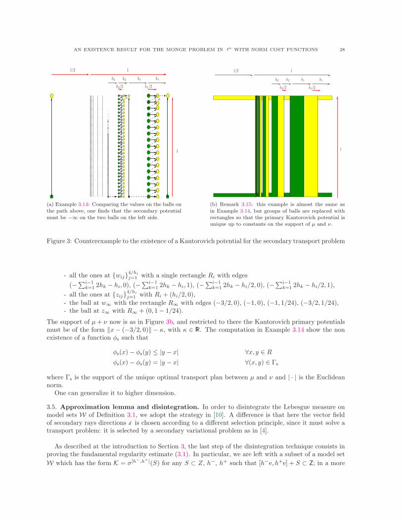
AN EXISTENCE RESULT FOR THE MONGE PROBLEM IN n WITH NORM COST FUNCTIONS 28
1/2 1
1
h1h1h2 h2
h1/2h2/2
( (
(a) Example 3.14: Comparing the values on the balls onthe path above, one finds that the secondary potentialmust be "& on the two balls on the left side.
1/2 1
1
h1h1h2 h2
h1/2h2/2
(b) Remark 3.15: this example is almost the same asin Example 3.14, but groups of balls are replaced withrectangles so that the primary Kantorovich potential isunique up to constants on the support of µ and ".
Figure 3: Counterexample to the existence of a Kantorovich potential for the secondary transport problem
- all the ones at {wij}4/hi
j=1 with a single rectangle Ri with edges
(#)i#1
k=1 2hk # hi, 0), (#)i#1
k=1 2hk # hi, 1), (#)i#1
k=1 2hk # hi/2, 0), (#)i#1
k=1 2hk # hi/2, 1),
- all the ones at {zij}4/hi
j=1 with Ri + (hi/2, 0),- the ball at w( with the rectangle R( with edges (#3/2, 0), (#1, 0), (#1, 1/24), (#3/2, 1/24),- the ball at z( with R( + (0, 1# 1/24).
The support of µ + ! now is as in Figure 3b, and restricted to there the Kantorovich primary potentialsmust be of the form !x# (#3/2, 0)! # 1, with 1 " . The computation in Example 3.14 show the nonexistence of a function "s such that
"s(x) # "s(y) ) |y # x| ,x, y " R
"s(x) # "s(y) = |y # x| ,(x, y) " $s
where $s is the support of the unique optimal transport plan between µ and ! and | · | is the Euclideannorm.
One can generalize it to higher dimension.
3.5. Approximation lemma and disintegration. In order to disintegrate the Lebesgue measure onmodel sets W of Definition 3.1, we adopt the strategy in [10]. A di"erence is that here the vector fieldof secondary rays directions d is chosen according to a di"erent selection principle, since it must solve atransport problem: it is selected by a secondary variational problem as in [4].
As described at the introduction to Section 3, the last step of the disintegration technique consists inproving the fundamental regularity estimate (3.1). In particular, we are left with a subset of a model set
W which has the form K = &[h!,h+](S) for any S + Z, h#, h+ such that [h#e, h+e] + S + Z; in a more

AN EXISTENCE RESULT FOR THE MONGE PROBLEM IN n WITH NORM COST FUNCTIONS 29
explicit way,
K =+
&t(z) : z " S, t " [h#, h+],
, &t(z) = z + td (z)
d (z) · ewhere S is a subset of {x · e = 0} such that r (z) · e ? [h#, h+].We have to show the push forward inequality
Hn#1(&t(S)) ).
t# h#
s# h#
/n#1
Hn#1(&s(S)) for h# < s ) t ) h+.
The estimate corresponding to the above one in [10] is proven is proven in Lemma 4.7, for the strictlyconvex case, and then in Lemma 5.7 for the general case. We follow here a similar limiting argument,providing on &s(S) a suitable approximation by vector fields d' which satisfy the regularity estimate andconverge pointwise to d !(s(S). Due to the di"erent limit, the vector field approximating d should bechosen di"erently from [10].Here comes the role of the secondary potential: it detects the secondary rays through a Hopf-Lax for-mula, and it consequently allows to view the vector field of secondary directions as pointwise limit ofapproximating directions which satisfy the regularity estimate.
The approximation lemma is the following.
Lemma 3.16. Fix h# < s ) t ) h+. Then there exist a sequence of vector fields {d'}' on Zt =K * {x · e = t} such that
- they converge pointwise to d on Zt;- they satisfy the push forward regularity estimate: for all compact St + Zt
Hn#1(St) ).
t# h#
s# h#
/N#1
Hn#1(&s#td#
St).
In a symmetric way, there exists a similar vector field on Zs = K * {x · e = s}, if h# ) s ) t < h+.
Proof. For y in Zt denote by x(y) the points on Zh! = K * {x · e1 = h#} belonging to the secondaryray through y; in particular, if y is an endpoint, then x can be multivalued. Let "s be the secondarypotential constructed in 3.13, which is by definition continuous on secondary transport rays of K. Sincewe are working up to countable partitions in compact sets, by Lusin theorem one can assume that "s iscontinuous on K.
Defining the functions
f(x, y) := "(y) # "(x) + !y # x!,
f %(x, y) :=
3
"s(y)# "s(x) + |y # x| if "(x) # "(y) = !y # x!+/ otherwise
thenx(y) = arg min
x$Zh!
f %(x, y) + arg minx$Zh!
f(x, y),
Consider moreover the functionals
f'(x, y) := "(y)# "(x) + !y # x! + )&
"s(y)# "s(x) + |y # x|'
,
f %'(x, y) :=
"(y) + !y # x! # "(x)
)+ "s(y)# "s(x) + |y # x|,
and define an approximating vector field of unit directions {d'}' from y to x'(y) by the formula
x'(y) := argminx$clos(Zh! )
f'(x, y).
Being on a bounded set, it is not di#cult to observe that for all fixed y " Zt
f(·, y) = $# lim'.0
f'(·, y) f %(·, y) = $# lim'.0
f %'(·, y).

AN EXISTENCE RESULT FOR THE MONGE PROBLEM IN n WITH NORM COST FUNCTIONS 30
Indeed, f'(x, y)# f(x, y) = )("s(y)# "s(x) + |y # x|) is uniformly bounded by 2 diam($s), while f %'(·, y)
increases pointwise to the continuous function f %(·, y).Then, from basic facts about $-convergence (see precisely recalls in Section 4 of [5]),
lim sup'.0
x'(y) = lim sup'.0
arg minx$Zh!
f'(x, y) 1 argminx$Zh!
f %(x, y) = x(y).
This proves that on Zh! any pointwise limit of the vector field {d'(y)}' belongs d (y).Call "'(y) := "(y) + )"s(y), and !·!' := !·!+ )| · |. Notice that !·!' is a strictly convex norm, and
x'(y) = arg min ("'(y)# "'(x) + !y # x!').
Then the approximation with countably many disjoint cones of Example 2.12 of [17] (already presentin [10]) shows that d' !K satisfies the push forward regularity estimate, following the argument ofLemma 2.13 itself, and by compactness of the sections one can pass to the limit, up to subsequences, bythe upper semicontinuity of the Hausdor" measure.
In a symmetric way, replace minimums with maximums and subtract, instead of adding, the norms tothe potentials. One finds then a vector field {d'(x)} on Zs converging to d (x) as ) $ 0, satisfying
Hn#1(Ss) ).
s# h#
t# h#
/n#1
Hn#1(&t#sd#
Ss) for all compact St + Zt. "
With the new approximation provided by Lemma 3.16, one can now follow the strategy explained inthe introduction of the section, at Page 18, and the accurate analogous computations are given fromLemma 2.13 to Lemma 2.21 in [17].
One arrives then at the following disintegration result.
Theorem 3.17. The following disintegration of Ln Ts strongly consistent with the covering {rq}q$Qholds:
Ln Ts =
!
Q
(' dH1rq) dHn#1(q)
where ' : n $ is strictly positive and Q is identified with a &-compact subset of countably manyhyperplanes. Moreover, ' !r q is locally Lipschitz continuous.
Corollary 3.18. The set of endpoints E is Ln-negligible.
Proof. If one applies the disintegration formula to the Borel set E , it is an immediate consequence ofH1(rq * E) = H1(rb(rq)) = 0. "
The Disintegration Theorm 3.17 and the estimates in Lemma 3.16 yield moreover a regularity propertyfor the divergence of the vector field of rays directions, as stated in Corollary 3.19 below.One can find di"erent proofs in Section 2.4 of [17] and Section 5.1 of [18]. The first argument waspresented in [10].
Corollary 3.19. Consider the notations defined in the introduction to the present section, Pages 18-21,
and define de = d (z)d (z)·ei
on the sets {Zi}i$ of a covering of the secondary transport set.
The divergence of the vector field dei of rays direction is a series of Radon measures. On sets K of theform
K =+
&t(z) : z " Si, t " [h#, h+],
where &t(z) = z + tdei(z)
the following divergence formula holds: for every - " C1c ( n)
:div dei ,-; =
!
K-(x)(div dei)a.c.(x) dLn(x) #
!
dK-(x) dei(x) · n(x) dHn#1(x),(3.11)

AN EXISTENCE RESULT FOR THE MONGE PROBLEM IN n WITH NORM COST FUNCTIONS 31
where dK, the border of K transversal to dei , is defined as K *Hh+ -K *Hh! , n(x) is the vector field ofunit directions normal to Hh+ -Hh! in the outer direction and
(div dei)a.c.(x) =%t.(t = #*ei+(x), x # x · ei dei(x))
.(#*ei+(x), x # x · ei dei(x)).
4. Notations
We group here some symbols one can find in the text. Standard ones are on the left, on the right the ones wedefined.
!·! a norm on n
| · | a norm on n whose unit ball is strictly convexBr(x) {x " n : |x| ) r}#a, b$ the segment from a to b without endpoints!a, b" the segment from a to b without endpointsrb(,) the relative boundary of a segment , consists in
the endpointsri(,) the relative interior of a segment , is , \ rb(,)1 the set inclusion6 the inclusion preserving the orientationX any subset of n
(X)c the complementary of Xclos(X) the closure of X in n
px the map px : n % n 5 (x, y) ($ x " n
py the map px : n % n 5 (x, y) ($ y " n
*X *X(x) = 1 if x " X , +/ otherwise
X X(x) = 1 if x " X , 0 otherwiseB(X) Borel &-algebra of XL (X) Lebesgue &-algebra of XM+
loc(X) positive and finite Radon measures on XM+(X) measures in M+
loc(X) with finite total variationP(X) Borel probability measures on XLn(X) Lebesgue (outer) measure of XHk(X) k-dimensional Hausdor" (outer) measure of X2 ' 3 if 2, 3 " M+
loc(X), 2 is absolutely continuousw.r.t. 3 if ,S " B(X) 3(S) = 0 implies 2(S) = 0
g! push forward with a map g%# subdi"erential%+ superdi"erential%#
c - {(x, y) : -(x) # -(y) = c(x, y)}
µ, ! µ, ! "M+( n) fixed, with µ ' Ln
!(µ, !) {# "M+( n % n) : px! (#) = µ, py
! (#) = !}Op see Page 4Os see Page 4" primary Kantorovich potential, (1.3)T primary transport set:
-{!x, y" : "(x) # "(y) = !y # x!}cs secondary cost function:
cs(x, y) = |y # x| {$(x)#$(y)=)y#x)}(x, y)G" see Definition 2.2 at Page 8r+" see Definition 2.2 at Page 8r" see Definition 2.2 at Page 8G%
" see (2.2) at Page 9r%+" see (2.2) at Page 9r%" see Remark 2.3rq, q, Q see Definition 2.4, Section 2.2, Lemma 2.11d see Definition 2.4, Section 2.2, Lemma 2.11Ts see Definition 2.4, Section 2.2, Lemma 2.11E# see Definition 2.4, Section 2.2E+ see Definition 2.4, Section 2.2E see Definition 2.4, Section 2.2F see Definition 2.4, Lemma 2.11$s a cs-monotone set, usually &-compact and con-
tained in {cs < +/}"s local secondary potential (Subsection 3.4)Z see Page 19Z see Page 19(, ., ' see Page 19, 19W see Section 3.1$ transport density, see (2.12)
Acknowledgements
The present work arises and has been developed thanks to many discussions, in first place with Prof. Ste-fano Bianchini. The author wishes to thank him for his help and the insights he gave into the problem,as well as for the constant support and availability.
She wishes moreover to thank Prof. Luigi Amrosio and Prof. Alessio Figalli for important suggestionsand several discussions when the author was visiting Scuola Normale and Centro De Giorgi. The workhas been finished while studying the related problem [18] with Sara Daneri.
All the mistakes are clearly introduced by me.

AN EXISTENCE RESULT FOR THE MONGE PROBLEM IN n WITH NORM COST FUNCTIONS 32
References
[1] G. Alberti, B. Kirchheim, and D. Preiss. Personal communication in [4].[2] L. Ambrosio. Lecture notes on optimal transport problems. In Mathematical aspects of evolving interfaces (Funchal,
2000), volume 1812 of Lecture Notes in Math., pages 1–52. Springer, Berlin, 2003.[3] L. Ambrosio, P. Cannarsa, and H. M. Soner. On the propagation of singularities of semi-convex functions. Annali della
scuola normale superiore di Pisa, 20(4):597–616, 1993.[4] L. Ambrosio, B. Kircheim, and A. Pratelli. Existence of optimal transport maps for crystalline norms. Duke Math. J.,
125(2):207–241, 2004.[5] L. Ambrosio and A. Pratelli. Existence and stability results in the L1 theory of optimal transportation. In Optimal
transportation and applications (Martina Franca, 2001), volume 1813 of Lecture Notes in Math., pages 123–160.Springer, Berlin, 2003.
[6] P. Appell. Memoire sur les deblais et les remblais des systemes continus ou discontinus. Memoires preesentes par diversSavants a l’Academie des Sciences de l’Institut de France, 29:1–208, 1887.
[7] M. Beckmann. A continuous model of transportation. Econometrica, 20:643–660, 1952.[8] S. Bianchini. On the Euler-Lagrange equation for a variational problem. Discrete Contin. Dyn. Syst., 17(3):449–480,
2007.[9] S. Bianchini and L. Caravenna. Su"cient conditions for optimality of c-cyclically monotone transference plans. In
preparation.[10] S. Bianchini and M. Gloyer. On the Euler Lagrange equation for a variational problem: the general case II. Preprint,
2007.[11] G. Bouchitte and G. Buttazzo. Characterization of optimal shapes and masses through Monge-Kantorovich equation.
J. Eur. Math. Soc. (JEMS), 3(2):139–168, 2001.[12] G. Bouchitte, G. Buttazzo, and Pierre Seppecher. Shape optimization solutions via Monge-Kantorovich equation. C.
R. Acad. Sci. Paris Ser. I Math., 324(10):1185–1191, 1997.[13] Y. Brenier. Decomposition polaire et rearrangement monotone des champs de vecteurs. C. R. Acad. Sci. Paris Ser. I
Math., 305(19):805–808, 1987.[14] Y. Brenier. Polar factorization and monotone rearrangement of vector-valued functions. Comm. Pure Appl. Math.,
44(4):375–417, 1991.[15] L. Ca!arelli, M. Feldman, and R. McCann. Constructing optimal mass for Monge’s transport problem as a limit of
strictly convex costs. J. Amer. Math. Soc., (15):1–26, 2002.[16] L. A. Ca!arelli. Boundary regularity of maps with convex potentials. II. Ann. of Math. (2), 144(3):453–496, 1996.[17] L. Caravenna. A proof of Sudakov theorem with strictly convex norms. Preprint, 2008.[18] L. Caravenna and S. Daneri. The disintegration of the lebesgue measure on the faces of a convex function. Preprint,
2009.[19] T. Champion and L. De Pascale. The Monge problem for strictly convex norms in d. to appear on Journ. of the Eur.
Math. Soc. in 2009.[20] T. Champion and L. De Pascale. The monge problem in d. Preprint, 2009.[21] C. Dupin. Applications de la geometrie et de la mecanique. 1822. re-edition by Bachelier, Paris.[22] L. C. Evans and W. Gangbo. Di!erential equations methods for the Monge-Kantorovich mass transfer problem. Current
Developments in Mathematics, pages 65–126, 1997.[23] M. Feldman and R. McCann. Monge’s transport problem on a Riemannian manifold. Trans. Amer. Math. Soc.,
(354):1667–1697, 2002.[24] M. Feldman and R. J. McCann. Uniqueness and transport density in Monge’s mass transportation problem. Calc. Var.
Partial Di!erential Equations, 15(1):81–113, 2002.[25] W. Gangbo. An elementary proof of the polar factorization of vector-valued functions. Arch. Rational Mech. Anal.,
128(4):381–399, 1994.[26] L. V. Kantorovich. On the transfer of masses. Docl. Akad. Nauk. SSSR, 37:227–229, 1942.[27] L. V. Kantorovich. On a problem of Monge. Uskpekhi Mat. Nauk., 3:225–226, 1948.[28] M. Knott and C. Smith. On the optimal mapping of distributions. J. Optim. Theory Appl., 43(1):39–49, 1984.[29] D. G. Larman. A compact set of disjoint line segments in 3 whose end set has positive measure. Mathematika,
18:112–125, 1971.[30] R. J. McCann. Existence and uniqueness of monotone measure-preserving maps. Duke Math. J., 80(2):309–323, 1995.[31] G. Monge. Memoire sur la Theorie des Deblais et des Remblais. Histoire de l’Acad. de Sciences de Paris, pages 666–704,
1781.[32] A. Pratelli. On the su"ciency of c-cyclically monotonicity for optimality of transport plans. Math. Z., 2007.[33] L. Ruschendorf and S. T. Rachev. A characterization of random variables with minimum L2-distance. J. Multivariate
Anal., 32(1):48–54, 1990.[34] F. Santambrogio. Absolute continuity and summability of transport densities: simpler proofs and new estimates. To
appear on Calc. Var. Par. Di!. Eq., 2008.[35] W. Schachermayer and J. Teichmann. Characterization of optimal Transport Plans for the Monge-Kantorovich-
Problem. Proceedings of the A.M.S., 2007. to appear.

AN EXISTENCE RESULT FOR THE MONGE PROBLEM IN n WITH NORM COST FUNCTIONS 33
[36] S. M. Srivastava. A course on Borel sets. Graduate texts in mathematics. New York Springer-Verlag, 1998.[37] V. N. Sudakov. Geometric problems in the theory of infinite-dimensional probability distributions. Proc. Steklov Inst.
Math., 2:1–178, 1979. Number in Russian series statements: t. 141 (1976).[38] N. S. Trudinger and X. J. Wang. On the Monge mass transfer problem. Calc. Var. PDE, (13):19–31, 2001.[39] C. Villani. Optimal Transport: Old and New, volume 338 of Grundlehren der mathematischen Wissenschaften.
Springer, 2009.
E-mail address: [email protected]
Laura Caravenna c/o SISSA, via Beirut 2-4, 34151 Trieste (TS), ITALY