n u m e r i c a l s t u d y - upcommonsupcommons.upc.edu/bitstream/handle/2117/86260/memoria.pdfy...
TRANSCRIPT

N U M E R I C A L S T U D Yand
O P T I M I Z A T I O Nof a GT Car Rear-Wing Aerodynamics
by
Masoud Arianezhad
Diploma Thesis for Degree
Master in Aerospace Science and Technology
at
Universitat Politecnica de Catalunya
Advisor:FERNANDO P. MELLIBOVSKY ELSTEIN
B a r c e l o n a , M a r c h 2 0 1 5

Dedicated to my motherThe most beautiful woman I have ever seen in my life.She is, to me, my rock.She is by far the strongest woman I have ever known.

Abstract
Race car performance significantly depends on elements such as the engine, tires, suspension, road,aerodynamics, and of course the driver. Although human factors are frequently publicized as thereason behind the success or failure of one racing team or another, engine power, tire adhesion,chassis design, and, aerodynamics probably play a more important role in winning the technologyrace. In recent years, however, vehicle aerodynamics gained increased attention, mainly due tothe utilization of the negative lift (downforce) principle, yielding several important performanceimprovements. Various methods exist to generate downforce such as inverted wings, diffusers, andvortex generators. Some cars like McLaren P1 are able to produce 600kg of downforce at well belowmaximum speed (257 km/h=161 mph) in Race mode, which is considerably higher than most otherhigh performance supercars, and more in line with the levels of downforce generated by a GT3 racingcar. This downforce improves the car s cornering ability, especially in high speed corners. Balance,agility and controllability are all outstanding.This work briefly explains the significance of the aerodynamic downforce by using multi-elementairfoils. After a short introduction, the philosophies behind the high-lift airfoils design are discussedand finally the CFD simulation of multi-element is performed and the resultant data is comparedand investigated.The first idea for this work was to design a new airfoil or optimize an available high-lift airfoilaccording to our requirements but since it needed to have a powerful inverse airfoil design softwarelike Profoil, which is not easy to access, and in addition the user should have a deep knowledge ofaerodynamics, we decided to choose some high-lift airfoils as the base and use their combinationfor CFD simulations. Unfortunately CFD simulations are so time consuming, for this reason manyresearchers try to simulate the multi-element airfoils in codes like MSES which is a numericalairfoil development system. It includes capabilities to analyze, modify and optimize single andmulti-element airfoils. But since we could not afford buying this relatively software, we tried to godirectly through CFD simulation of multi-element airfoils. Unfortunately, it is hard to find empiricaldata about rear wing of race cars because normally they are confidential piece of information of bigcar companies. On the other hand it is so rare to find a similar wind tunnel or CFD simulationof the same selected multi-element airfoils and what can be found is almost always empirical dataof single element airfoils. All these things make it hard to have a reliable CFD results as long asthere is no evaluation of results with the real world information. It would be interesting that in thefuture someone use information of this work as a reference to compare with wind tunnel or CFDsimulations.


Contents
1 Introduction 9
1.1 Aerodynamic Downforce . . . . . . . . . . . . . . . . . . . . . . . . . 9
1.2 Airfoil Force and Moment Coefficients . . . . . . . . . . . . . . . . . 11
1.2.1 Types of Drag . . . . . . . . . . . . . . . . . . . . . . . . . . 12
1.3 Technical Regulations for Grand Touring Cars . . . . . . . . . . . . 13
1.4 Structure of the Thesis . . . . . . . . . . . . . . . . . . . . . . . . . . 13
2 Design Methodology 15
2.1 High Lift Design Philosophy . . . . . . . . . . . . . . . . . . . . . . . 16
2.2 S1223 High Lift Section . . . . . . . . . . . . . . . . . . . . . . . . . 18
2.3 Eppler E420 airfoil . . . . . . . . . . . . . . . . . . . . . . . . . . . . 19
2.4 Blunt or Flatback Trailing Edge . . . . . . . . . . . . . . . . . . . . 20
2.5 S1223 (with blunt trailing edge) Performance . . . . . . . . . . . . . 20
2.6 Multi-element Airfoils . . . . . . . . . . . . . . . . . . . . . . . . . . 21
2.6.1 The Flap Effect . . . . . . . . . . . . . . . . . . . . . . . . . . 23
2.6.2 Fresh Boundary-Layer Effect . . . . . . . . . . . . . . . . . . 24
2.7 Boundary-Layer Separation . . . . . . . . . . . . . . . . . . . . . . . 25
3 Computational Fluid Dynamics (CFD) Modeling 27
3.1 Geometry . . . . . . . . . . . . . . . . . . . . . . . . . . . . . . . . . 27
3.2 Turbulence Model . . . . . . . . . . . . . . . . . . . . . . . . . . . . 28
3.2.1 SST k-ω Model . . . . . . . . . . . . . . . . . . . . . . . . . . 30
3.3 Grid Generation . . . . . . . . . . . . . . . . . . . . . . . . . . . . . 31
3.3.1 Structured or Unstructured Grids? . . . . . . . . . . . . . . . 31
3.3.2 Boundary Layer and Estimation of First Cell Height for cor-rect y+ (Wall Unit) . . . . . . . . . . . . . . . . . . . . . . . 32
3.3.3 Grid Resolution for RANS Models . . . . . . . . . . . . . . . 34
3.3.4 Domain Boundaries and Grids . . . . . . . . . . . . . . . . . 35
3.3.5 Near-wall Mesh Generation . . . . . . . . . . . . . . . . . . . 36
3.4 Multi-Element Airfoil Configuration . . . . . . . . . . . . . . . . . . 38
3.5 Set up the solver (Ansys Fluent) and physical models . . . . . . . . 40

ii CONTENTS
3.5.1 The Pressure-Based Segregated Algorithm . . . . . . . . . . . 413.5.2 Transient Solution . . . . . . . . . . . . . . . . . . . . . . . . 42
4 CFD Simulation Results 454.1 2D Single Airfoil . . . . . . . . . . . . . . . . . . . . . . . . . . . . . 46
4.1.1 Boundary Conditions . . . . . . . . . . . . . . . . . . . . . . 464.1.2 Results . . . . . . . . . . . . . . . . . . . . . . . . . . . . . . 464.1.3 Grid Independence Study . . . . . . . . . . . . . . . . . . . . 47
4.2 2D Multi-element Airfoil . . . . . . . . . . . . . . . . . . . . . . . . . 494.2.1 Flap Deflection αf = 40o: . . . . . . . . . . . . . . . . . . . . 494.2.2 Flap Deflection αf = 35o: . . . . . . . . . . . . . . . . . . . . 49
4.3 Discussion . . . . . . . . . . . . . . . . . . . . . . . . . . . . . . . . . 524.3.1 Effect of Turbulence Models on the Results . . . . . . . . . . 584.3.2 Separation Bubbles . . . . . . . . . . . . . . . . . . . . . . . . 594.3.3 Variation of Angle of Attack and Multi-element Airfoil Perfor-
mance . . . . . . . . . . . . . . . . . . . . . . . . . . . . . . . 624.3.4 Karman vortex street . . . . . . . . . . . . . . . . . . . . . . 654.3.5 Effect of Variation of Sportscar Speed . . . . . . . . . . . . . 65
5 Conclusions 695.1 Future works . . . . . . . . . . . . . . . . . . . . . . . . . . . . . . . 71
5.1.1 3D Wing Simulation . . . . . . . . . . . . . . . . . . . . . . . 715.1.2 Analysis of Twisted Wing . . . . . . . . . . . . . . . . . . . . 72
Conclusions 69
A Some Aerodynamics Definitions 73

Acknowledgments
I would like to thank my family and specially my beloved mother for their constantsupport. Without their help it would impossible to continue my study here in Spainand overcome a challenging student s life in a foreign country on a limited budgetand many other emotional and social difficulties. Nobody would understand thetoughness of living abroad until they try it.
Unfortunately my father is not among us anymore. I also like to thank him forbringing me up like a strong man. May God bless his soul and rest him in peace
I would also like to appreciate all kind helps of my supervisor FERNANDO MEL-LIBOVSKY ELSTEIN. Without his supervision and great recommendations thisproject could go to a wrong direction.
I would also like to thank my friends for their support during my staying in Spain.They help me to feel like I am in my own country.


List of Figures
1.1 Variation of the one-lap record speed at the Indianapolis Speedway.[1] 9
2.1 A graph demonstrates the Interrelation between boundary layer con-trol efforts and consequences. . . . . . . . . . . . . . . . . . . . . . . 17
2.2 Pressure distribution vectors computed from XFOIL for α = 5o showairfoil loading. Note that the vectors with arrows pointed outwardcorrespond to relatively negative pressure. . . . . . . . . . . . . . . . 18
2.3 Trends in low Reynolds number airfoil characteristics as functionsof the pitching moment and type of upper-surface pressure recoverydistributions. (adopted from [2]) . . . . . . . . . . . . . . . . . . . . 19
2.4 Plot comparing modified T.E airfoil with original S1223 airfoil. . . . 21
2.5 A Comparison between lift coefficient of original S1223 airfoil andS1223 with trailing edge gap of 0.5% of the chord length.(The viscous
analysis has been done in XFOIL for Re=800,000) . . . . . . . . . . . . . . . 22
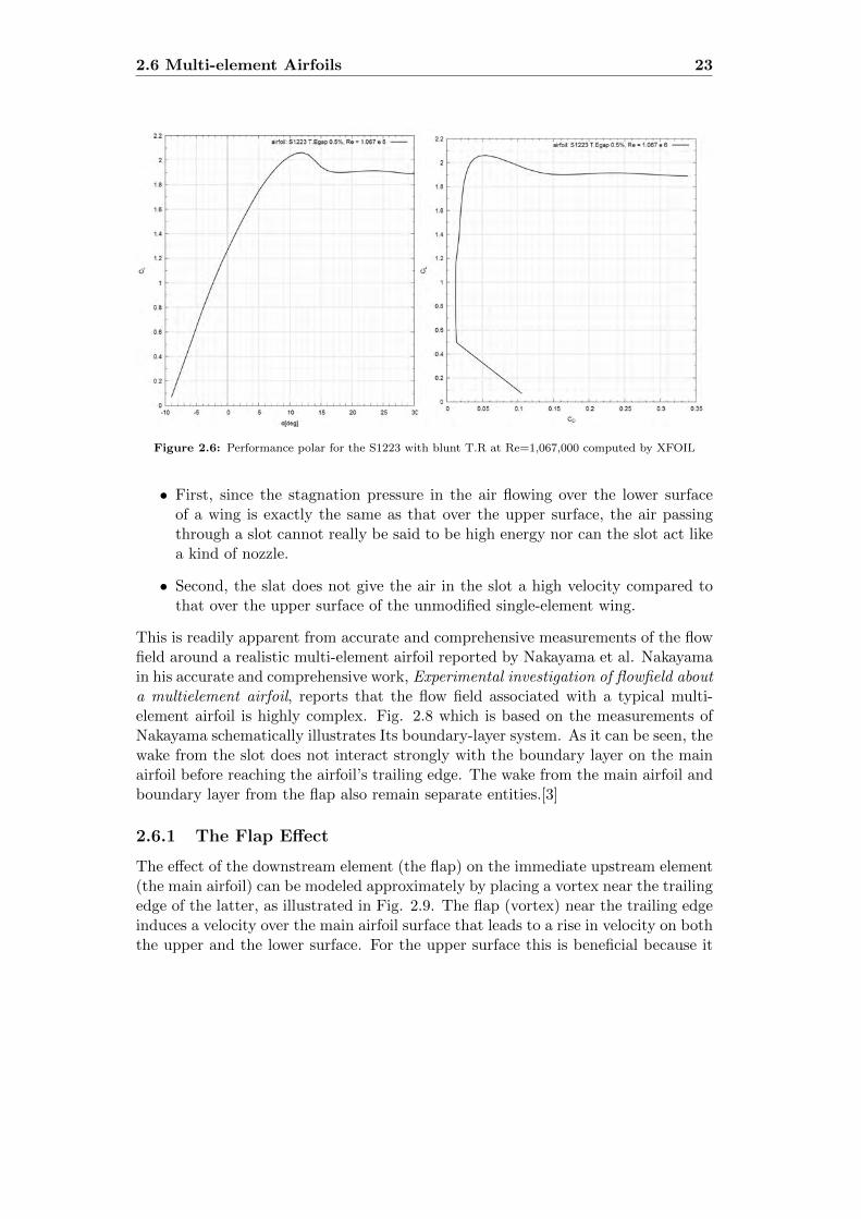
2.6 Performance polar for the S1223 with blunt T.R at Re=1,067,000computed by XFOIL . . . . . . . . . . . . . . . . . . . . . . . . . . . 23
2.7 Performance comparison in different Reynolds numbers computed byXFOIL . . . . . . . . . . . . . . . . . . . . . . . . . . . . . . . . . . . 24
2.8 Typical boundary-layer behavior for a three-element airfoil.[3] . . . . 25
2.9 Flap effect (modeled by a vortex) on the velocity distribution over themain wing. . . . . . . . . . . . . . . . . . . . . . . . . . . . . . . . . 26
2.10 Boundary layer developing around an airfoil. . . . . . . . . . . . . . 26
3.1 A Screen shot from XFOIL of Mark Drela showing its root menu . . 29
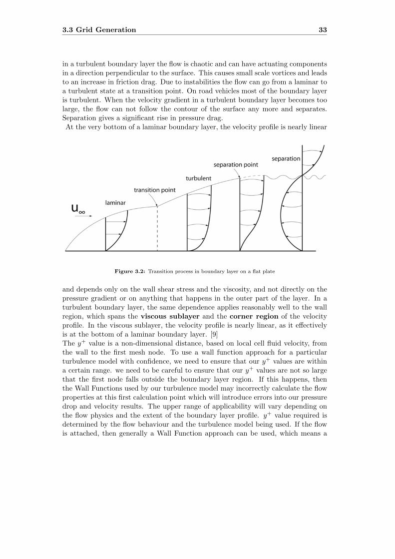
3.2 Transition process in boundary layer on a flat plate . . . . . . . . . 33
3.3 Domain boundary distances were chosen as 16.5× (total Chord Length)for the inlet and 30× (total Chord Length) for the outlet . . . . . . . 36
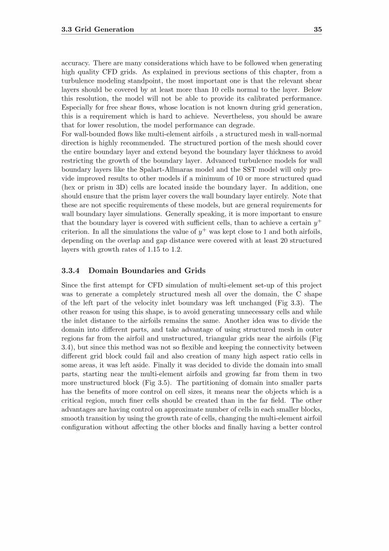
3.4 Hybrid mesh used as the first attempt for creating grids in which themajority of it (except close to multi-element airfoil) contains struc-tured mesh, however finally a completely unstructured mesh was chosen. 37
3.5 Division of domain into smaller parts. . . . . . . . . . . . . . . . . . 38
2 LIST OF FIGURES
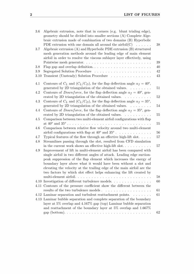
3.6 Algebraic extrusion, note that in corners (e.g. blunt trialing edge),geometry should be divided into smaller sections (A) Complete Alge-braic extrusion made of combination of two domains (B) HyperbolicPDE extrusion with one domain all around the airfoil(C) . . . . . . 38
3.7 Algebraic extrusion (A) and Hyperbolic PDE extrusion (B) structuredmesh generation methods around the leading edge of main elementairfoil in order to resolve the viscous sublayer layer effectively, usingPointwise mesh generator. . . . . . . . . . . . . . . . . . . . . . . . . 39
3.8 Flap gap and overlap definition. . . . . . . . . . . . . . . . . . . . . . 40
3.9 Segregated Solution Procedure . . . . . . . . . . . . . . . . . . . . . 42
3.10 Transient (Unsteady) Solution Procedure . . . . . . . . . . . . . . . 43
4.1 Contours of CL and (CL/CD), for the flap deflection angle αf = 40o,generated by 2D triangulation of the obtained values. . . . . . . . . 51
4.2 Contours of Downforce, for the flap deflection angle αf = 40o, gen-erated by 2D triangulation of the obtained values. . . . . . . . . . . 52
4.3 Contours of CL and (CL/CD), for the flap deflection angle αf = 35o,generated by 2D triangulation of the obtained values. . . . . . . . . 54
4.4 Contours of Downforce, for the flap deflection angle αf = 35o, gen-erated by 2D triangulation of the obtained values. . . . . . . . . . . 55
4.5 Comparison between two multi-element airfoil configurations with flapat 40o and 35o . . . . . . . . . . . . . . . . . . . . . . . . . . . . . . . 55
4.6 Comparison between relative flow velocity around two multi-elementairfoil configurations with flap at 40o and 35o . . . . . . . . . . . . . 56
4.7 Typical features of the flow through an effective high-lift slot. . . . . 57
4.8 Streamlines passing through the slot, resulted from CFD simulationin the current work shows an effective high-lift slot. . . . . . . . . . . 57
4.9 Improvement of lift in multi-element airfoil has been compared withsingle airfoil in two different angles of attack. Leading edge suction-peak suppression of the flap element which increases the energy ofboundary layer above what it would have been without a slot andelevating the velocity at the trailing edge of the main airfoil are thetwo factors by which slot effect helps enhancing the lift created bymulti-element airfoil. . . . . . . . . . . . . . . . . . . . . . . . . . . . 58
4.10 Investigation of different turbulence models. . . . . . . . . . . . . . . 60
4.11 Contours of the pressure coefficient show the different between theresults of the two turbulence models . . . . . . . . . . . . . . . . . . 61
4.12 Laminar separation and turbulent reattachment points. . . . . . . . 61
4.13 Laminar bubble separation and complete separation of the boundarylayer at 5% overlap and 4.167% gap (top) Laminar bubble separationand reattachment of the boundary layer at 5% overlap and 1.667%gap (bottom). . . . . . . . . . . . . . . . . . . . . . . . . . . . . . . . 62

LIST OF FIGURES 3
4.14 Comparison between the resultant pressure coefficient plot at (5%overlap and 4.167% gap) and t (5% overlap and 1.667% gap). . . . . 63
4.15 Variation of the angle of attack for αf = 40o multielement configura-tion. . . . . . . . . . . . . . . . . . . . . . . . . . . . . . . . . . . . 67
4.16 Formation of Karman vortex street in wake of the multi-element airfoilin αf = 35o configuration. . . . . . . . . . . . . . . . . . . . . . . . . 68
5.1 3D mesh around 25% of the wing including the endplate. . . . . . . 715.2 3D domain around 25% of the wing including the endplate. . . . . . 72
A.1 Airfoil (wing section) geometry and definitions. . . . . . . . . . . . . 73A.2 Typical pressure distributions on an airfoil section. . . . . . . . . . . 74A.3 Pressure Distribution over NACA 4410 airfoil at α = 2◦ . . . . . . . 75


List of Tables
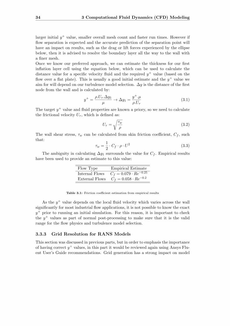
3.1 Friction coefficient estimation from empirical results . . . . . . . . . 34
4.1 Main airfoil simulations (Single Element S1223) at 0o and 5o andRe=1.1×10⁶ . . . . . . . . . . . . . . . . . . . . . . . . . . . . . . . . 47
4.2 CFD simulation results of Multi-element airfoil. The main airfoilis Selig S1223 that has chord length of 240mm. The flap airfoil,Eppler E420 with chord length of 84mm, was kept at fixed αf =40o. Both airfoils have 0.5% gap at their trailing edges. Turbu-lence model in all simulations is the two-equation model, SST K-ω.Highlighted areas are correspondent for the CL,max. , (CL/CD)max.and max. Downforce. O.L = ( overlap distance
main airfoil chord length)% and Gap =
( Gap distancemain airfoil chord length)%. . . . . . . . . . . . . . . . . . . . . . . . 50
4.3 CFD simulation results of Multi-element airfoil. The main airfoilis Selig S1223 that has chord length of 240mm. The flap airfoil,Eppler E420 with chord length of 84mm, was kept at fixed αf =35o. Both airfoils have 0.5% gap at their trailing edges. Turbu-lence model in all simulations is the two-equation model, SST K-ω.Highlighted areas are correspondent for the CL,max. , (CL/CD)max.and max. Downforce. O.L = ( overlap distance
main airfoil chord length)% and Gap =
( Gap distancemain airfoil chord length)%. . . . . . . . . . . . . . . . . . . . . . . . 53
4.4 Grid Independence Study for Multi-Element airfoil . . . . . . . . . . 534.5 CFD simulation results of Multi-element airfoil with flap position at
αf = 40o, in different aoa while both airfoils are rotated around theleading edge of the main element airfoil . . . . . . . . . . . . . . . . 64
4.6 CFD simulation results of Multi-element airfoil with flap position atαf = 35o, in different aoa while both airfoils are rotated around theleading edge of the main element airfoil . . . . . . . . . . . . . . . . 64
4.7 CFD simulation results of Multi-element airfoil with flap position atαf = 40o, in different aoa while both airfoils are rotated around theleading edge of the main element airfoil . . . . . . . . . . . . . . . . 66


Nomenclature
CD airfoil section drag coefficientCL airfoil section lift coefficientCf airfoil section skin friction coefficientα angle of attackaoa or AOA angle of attackαf flap deflection of multi-element airfoilCL wing lift coefficientClmax maximum airfoil lift coefficientm.c main airfoil chord lengthO.L multi-element airfoil overlappingRe Reynolds Numberν kinematic viscosity (µ/ρ)∞ undisturbed flowV∞ freestream velocityCFD computational fluid dynamicsSST k − ω Two-equation, Menter s Shear Stress Transport k-omega Turbulence ModelSST k − ε k-epsilon Turbulence Model


Chapter 1
Introduction
1.1 Aerodynamic Downforce
Since the early days of the automobile and of motor racing, engine, tire, and suspen-sion technology have gradually developed. In most of these disciplines the advanceswere reasonably gradual, leading to increased race car performance, higher speeds,and lower lap times. This trend is demonstrated by Fig 1.1 , which shows the his-tory of the one-lap record speed at the Indianapolis Speedway. As can be seen, thebiggest jump in speed occurred in 1972 with the first efficient use of front and rearwings.[1]
Figure 1.1: Variation of the one-lap record speed at the Indianapolis Speedway.[1]
In addition to improved cornering speeds, aerodynamics have dramatically im-proved vehicle stability and high-speed braking as well, which again lead to faster
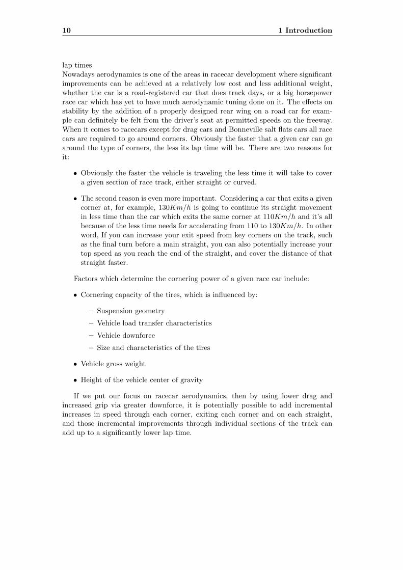
10 1 Introduction
lap times.Nowadays aerodynamics is one of the areas in racecar development where significantimprovements can be achieved at a relatively low cost and less additional weight,whether the car is a road-registered car that does track days, or a big horsepowerrace car which has yet to have much aerodynamic tuning done on it. The effects onstability by the addition of a properly designed rear wing on a road car for exam-ple can definitely be felt from the driver’s seat at permitted speeds on the freeway.When it comes to racecars except for drag cars and Bonneville salt flats cars all racecars are required to go around corners. Obviously the faster that a given car can goaround the type of corners, the less its lap time will be. There are two reasons forit:
• Obviously the faster the vehicle is traveling the less time it will take to covera given section of race track, either straight or curved.
• The second reason is even more important. Considering a car that exits a givencorner at, for example, 130Km/h is going to continue its straight movementin less time than the car which exits the same corner at 110Km/h and it’s allbecause of the less time needs for accelerating from 110 to 130Km/h. In otherword, If you can increase your exit speed from key corners on the track, suchas the final turn before a main straight, you can also potentially increase yourtop speed as you reach the end of the straight, and cover the distance of thatstraight faster.
Factors which determine the cornering power of a given race car include:
• Cornering capacity of the tires, which is influenced by:
– Suspension geometry
– Vehicle load transfer characteristics
– Vehicle downforce
– Size and characteristics of the tires
• Vehicle gross weight
• Height of the vehicle center of gravity
If we put our focus on racecar aerodynamics, then by using lower drag andincreased grip via greater downforce, it is potentially possible to add incrementalincreases in speed through each corner, exiting each corner and on each straight,and those incremental improvements through individual sections of the track canadd up to a significantly lower lap time.

1.2 Airfoil Force and Moment Coefficients 11
The first and most obvious approach to create downforce is to use invertedairplane-like wings to create downforce instead of lift. Such inverted wings can befound throughout the whole spectrum of automobile racing. While various compo-nents of an aerodynamic package contribute differently to the downforce levels andresulting flow fields, only the front and rear airfoils and wings lend themselves totheoretical aerodynamic analysis methods and techniques for design. Other compo-nents and body shape designs still rely on experimental and numerical data at thedesign stage.
1.2 Airfoil Force and Moment Coefficients
A discussion on wings traditionally starts with a discussion on the wing section shape,the airfoil. Following this approach and first demonstrate the aerodynamic signifi-cance of the airfoil geometry and its effect on lift and drag. A three-dimensional wingconsists of airfoil sections, but the shape of the wing planform in terms of sweep,taper, twist, and other geometrical parameters affects the overall performance aswell. In another definition an airfoil is the two-dimensional cross section of a three-dimensional wing.The nondimensional quantity called a force coefficient, F/(V 2S) where F is an aero-dynamic force and S is an area. is similar to the type often developed and usedin aerodynamics. It is not, however, used in precisely this form. In place of ρV 2
it is conventional for incompressible flow to use 12ρV
2, the dynamic pressure of thefree-stream flow. The actual physical area of the body, such as the planform areaof the wing is usually used for S. Thus the aerodynamic force coefficient is usuallydefined as follows:
CF =F
12ρV
2S(1.1)
The two most important force coefficients are lift and drag, defined by:
Lift Coefficient CL =Lift
12ρV
2S(1.2)
Drag Coefficient CD =Drag
12ρV
2S(1.3)
When the body in question is a wing, the area S is almost invariably the planform.Airfoil Moment: The aerodynamic lift and drag are the result of integrating thesurface pressure distribution. It is possible to represent the resultant force due tothis pressure distribution by a single force F . One of the more interesting conclusionsfrom basic airfoil theory is that this force acts at the quarter chord of a symmetricairfoil and points in the lift direction. Consequently, this point, called the center ofpressure. For cambered wings the center of pressure can be in a different location

12 1 Introduction
and may vary with angle of attack, whereas the aerodynamic center will be near thequarter chord.For race car applications the location of the aerodynamic center is less significant,while the location of the center of pressure is more important; a small backwardshift of the center of pressure on the rear wing of a race car can visibly influenceperformance.
1.2.1 Types of Drag
Total DragTotal drag is formally defined as the force corresponding to the rate of decrease inmomentum in the direction of the undisturbed external flow around the body. Thisdecrease is calculated between stations at infinite distances upstream and down-stream of the body, so it is the total force or drag in the direction of the undisturbedflow. It is also the total force resisting the motion of the body through the surround-ing fluid. There are a number of separate contributions to total drag. As a first stepit may be divided by physical effect into pressure drag and skin-friction drag.
Skin-Friction Drag (or Surface-Friction Drag:) Skin-friction drag is gen-erated by the resolved components of the traction due to shear stresses acting onthe body surface. This traction is due directly to viscosity and acts tangentially atall points on the body surface. At each point it has a component aligned with butopposing the undisturbed flow (i.e., opposite to the direction of flight). The totaleffect of these components, integrated over the entire exposed surface of the body,is the skin-friction drag. Skin-friction drag cannot exist in an invisicid flow.Pressure Drag: Pressure drag is generated by the resolved components of theforces due to pressure acting normal to the surface at all points. It is computed asthe integral of the flight-path direction component of the pressure forces acting onall points on the body. Pressure distribution, and thus pressure drag, has severaldistinct contributions:
• Induced drag (sometimes known as drag due to lift or vortex drag).
• Wave drag, when there exists a supersonic region in the flow regardless of theflight Mach number being less than or greater than 1.
• Form drag (sometimes known as boundary-layer pressure drag).
The Wake: Behind any body moving in air is a wake. Although the wake in airis not normally visible, it may be felt, as when, for example, a bus passes by. Thetotal drag of a body appears as a loss of momentum and an increase of energy in thewake. The loss of momentum appears as a reduction of average flow speed, while theincrease of energy is seen as violent eddying (or vorticity). The size and intensity ofthe wake is therefore an indication of the profile drag of body.

1.3 Technical Regulations for Grand Touring Cars 13
1.3 Technical Regulations for Grand Touring Cars
While the benefits of inverted rear and front wings were understood by racers andmany racing-sanctioning organizations recognized the strong influence of aerody-namics on lap-speed they attempted to create regulations based on placing limitson the use and size of aerodynamic devices such as inverted wings. Similarly, theACO ( Automobile Club de l’Ouest) has defined limits and requirements for theaerodynamic devices of LM GTE (Le Mans Grand Touring Endurance) category areas below:
• A wing made from one element only is permitted on top of the bodyworkprovided that: It replaces the original rear wing if one is fitted on the car;
• It fits, including end plates and angle bracket, into a volume the dimensions ofwhich are 45 cm (horizontal) x 15 cm (vertical) x 91% of the maximum widthof the road car homologated (ACO Homologation Form);
• The chord of the wing section not to exceed 30 cm;
• It is set forward by 5 cm in relation to the rearmost point of the bodywork.Any bodywork modification or extension the purpose of which is to move thewing backward is prohibited;
• It is set 10 cm lower than the highest point of the roof.[4]
Despite the above mentioned rules, there are many other categories of GT racecarswhich have less restrictions and designers are allowed to use multi-element (mostlydual element) wings and different endplate shapes. In this project we try to ignoreLe Mans restricted rules for using single-element wing and instead we will design adual element wing, however the dimensional restrictions will be applied as mandatedby ACO.
1.4 Structure of the Thesis
In the next chapter firstly the design available philosophies of high-lift airfoil willbe discussed and then the two airfoils which are selected as main and flap airfoilsfor this project will be introduced and compared with other famous high-lift airfoils.In continue of the next chapter the benefit of the blunt trailing edge (T.E) will beexplained and the resultant simulation in XFOIL will be discussed. Then, at theend of Chapter 2 we become familiar with multi-element airfoils and the role of slotwhich is known as slot effect will be explained. Finally we will be introduced to ashort explanation about separation of flow on airfoils.Chapter 3 mostly deals with the fundamental works of CFD simulation, however thebeginning of this chapter will be the explanation of how the geometries of airfoils

14 1 Introduction
were imported to the computer, modified, initially simulated and finally prepared formesh generator software and CFD solver. Later the most important part of a CFDwork which is mesh generation will be discussed and we will realized the advantageand disadvantages of different commonly used meshes (grids) in CFD. After thispart which is an introduction to meshing techniques, the method used in this workis explained. Because in this work it is assumed that the freestream is completelyturbulent, selection of the turbulence model is of great importance; for this reasonthe selected turbulence model will be introduced and compared to others. Finallythe set-up af the CFD solver and solution method will be described.Chapter 4 which is the most important part of this work, is the result of the CFDsimulations. First we see the CFD results of the single element to have a rough guessabout the accuracy of the solution, number of cells, solver st-up etc.. Next we startsimulation of the multi element airfoil in two different flap deflections, αf = 35o andαf = 40o. When the optimum points of each configuration is obtained, these twopoint will be compared. In addition accuracy of the simulation will be explainedand the method is described. Because of changing in speed of the car and aoa of theupcoming air, rearwing should be able to operate perfectly in different conditions,for this reason, various simulations in different speeds and aoa were performed.Last chapter is the conclusion of the thesis and brief explanation of what has beendone in this work. Finally the future works will be suggested.

Chapter 2
Design Methodology
However in this project the goal is not to design a high-lift airfoil used in race cars,but it is important to have the knowledge of its design so the candidate airfoils will bechosen precisely. Airfoil design methodologies that satisfying complex requirementsof racecars wings are confidential pieces of information that teams and other tech-nical organizations rarely publish their precious secrets and experiments in booksor journals and as a consequence the wing design in this field is based on theory,experimental data and sometimes guesses. Like most of airfoil design problem, thecommon goal of a race car wing is to generate as much lift Clmax (actually down-force) as possible within the physical constraints of the permissible dimensions of thewing.[5] While achieving this goal, various other criteria can be taken into accountin the design process to guarantee proper functioning of the high downforce systemunder available constraints associated with motorsports applications.The process is involving of choosing the pressure distribution, particularly that onthe upper wing surface, to maximize lift is the base of the high-lift airfoils design.Even when a completely satisfactory answer is found to this rather difficult issue, itstill remains to determine the appropriate shape of the airfoil to produce the spec-ified pressure distribution. This second step in the process is the so-called inverseproblem of airfoil design. It is much more demanding than the direct problem ofdetermining the pressure distribution for a given airfoil shape.[3] Nevertheless, sat-isfactory inverse design methods are available, although they will not be discussedhere. In broad terms the maximum lift achievable is limited by two factors:
• Boundary-layer separation
• The onset of supersonic flow
As long as here we are only interested in subsonic flow, the second factor will not bediscussed.In two-dimensional flow, boundary-layer separation is governed by:
• The severity and quality of the adverse pressure gradient
16 2 Design Methodology
• The kinetic-energy defect in the boundary layer at the start of the adversepressure gradient
In the next part the practical affect of the quality of adverse pressure and its impor-tance in a good high-lift design philosophy will be discussed more.
2.1 High Lift Design Philosophy
The different design philosophies in the low to moderate Reynolds number regimeinclude the approaches used by Liebeck, Eppler, Wortmann and Selig. To study andimplement the applicability of aft loading to motorsports applications, it is necessaryto understand the interdependence of various airfoil characteristics upon one another.A graphic representation of the various flow boundary layer transition regimes andthe performance consequences is demonstrated in Fig 2.1.It is well known that as pitching moment increases, maximum lift coefficient in-creases along with the pressure recovery becoming convex (Fig 2.3). Other observ-able trends from the same figure indicate that as an airfoil tends towards a moreconcave loading, high lift is achievable along with an increase in the rapidity withwhich stall is reached. Liebeck airfoils are a good example of the first type wherea large rooftop/suction level is employed followed by a Stratford pressure recovery(or concave pressure recovery). This leads to hard stall characteristics and high liftwith low pitching moment.The second approach is that reflected by some of the Wortmann airfoils where thereliance on a suction peak is reduced and more emphasis is placed on aft loading(convex pressure recovery) in order to provide softer stall characteristics.A third, middle ground, methodology is reflected by the Selig and Eppler high liftairfoils where a combination of the aforementioned design philosophies are utilizedin combination to provide high lift at low Reynolds number.The Liebeck airfoils rely on a Stratford boundary-layer inverse solution whereby apressure recovery distribution can be found that continuously avoids separation ofthe turbulent boundary layer. It is meant to recover the maximum possible pressurerise in the shortest possible distance. The Stratford recovery also represents theoptimum distribution for low profile drag and this leads to some of the highest liftto drag ratios for these class of airfoils. But this makes the boundary layer on theupper surface very sensitive to surface imperfections that may trip the flow.Motorsport applications often have wings positioned close to the ground. Even rearwings have surfaces that are constantly closer to the ground than typically found inaeronautical applications and this makes their surfaces susceptible to various bits oftrack and tire debris. These particles can potentially act as trips and, in the case ofairfoils reliant on Stratford recoveries, may influence the potential to generate highdownforce.Eppler argued that the sensitivity of the turbulent boundary layer in a Stratford
2.1 High Lift Design Philosophy 17
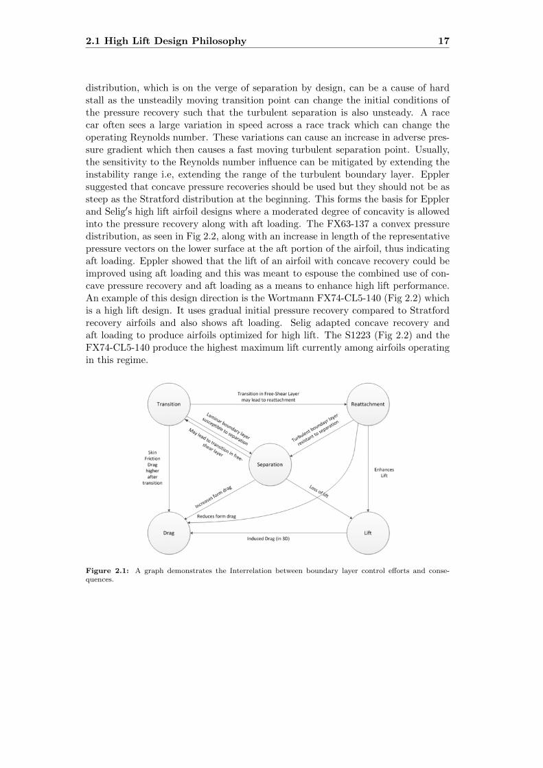
distribution, which is on the verge of separation by design, can be a cause of hardstall as the unsteadily moving transition point can change the initial conditions ofthe pressure recovery such that the turbulent separation is also unsteady. A racecar often sees a large variation in speed across a race track which can change theoperating Reynolds number. These variations can cause an increase in adverse pres-sure gradient which then causes a fast moving turbulent separation point. Usually,the sensitivity to the Reynolds number influence can be mitigated by extending theinstability range i.e, extending the range of the turbulent boundary layer. Epplersuggested that concave pressure recoveries should be used but they should not be assteep as the Stratford distribution at the beginning. This forms the basis for Epplerand Selig′s high lift airfoil designs where a moderated degree of concavity is allowedinto the pressure recovery along with aft loading. The FX63-137 a convex pressuredistribution, as seen in Fig 2.2, along with an increase in length of the representativepressure vectors on the lower surface at the aft portion of the airfoil, thus indicatingaft loading. Eppler showed that the lift of an airfoil with concave recovery could beimproved using aft loading and this was meant to espouse the combined use of con-cave pressure recovery and aft loading as a means to enhance high lift performance.An example of this design direction is the Wortmann FX74-CL5-140 (Fig 2.2) whichis a high lift design. It uses gradual initial pressure recovery compared to Stratfordrecovery airfoils and also shows aft loading. Selig adapted concave recovery andaft loading to produce airfoils optimized for high lift. The S1223 (Fig 2.2) and theFX74-CL5-140 produce the highest maximum lift currently among airfoils operatingin this regime.
Figure 2.1: A graph demonstrates the Interrelation between boundary layer control efforts and conse-quences.

18 2 Design Methodology
Figure 2.2: Pressure distribution vectors computed from XFOIL for α = 5o show airfoil loading. Note thatthe vectors with arrows pointed outward correspond to relatively negative pressure.
2.2 S1223 High Lift Section
Based on an analysis of several high lift sections, Fig 2.3 shows the pitching momentcharacteristics vs. the type of upper-surface pressure recovery for several airfoils. TheFX 63-137 with its relatively high (negative) pitching moment and convex pressurerecovery appears towards the upper left corner. In contrast, airfoils with a Stratford-like concave pressure recoveries and low pitching moments, such as the Miley M06-13-128 airfoil, appear on the lower right. It should be noted that the figure is used toonly illustrate the trends and qualitative ideas. Thus, it is not intended to be whollyaccurate with respect to the placement of the airfoils. For instance, two airfoils canhave the same pitching moment and similar recovery distributions and hence occupythe same point on the plot, yet these two airfoils could exhibit different camber,Clmax and stall characteristics. In the figure, the airfoils are placed most accuratelywith respect to the Clmax and shape of the recovery distribution. The WortmannFX74-Cl5-140 and the Selig S1223 show very similar behavior. They have bothbeen designed on similar principles, although historically, the Wortmann airfoil wasdesigned for higher Reynolds number close to 1000000 and the S1223 was designedfor an operating Reynolds number range between 200,000 to about 800,000 howeverit still works satisfactorily for Reynolds numbers near 1,200,000. This wide range ofReynolds numbers makes S1223 airfoil a good candidate for rear wing of sportcars dueto the variation of speed of the car on track , and of course, variation in Reynolds

2.3 Eppler E420 airfoil 19
number. One trend depicted in Fig 2.3 is that an airfoil typically becomes more
Figure 2.3: Trends in low Reynolds number airfoil characteristics as functions of the pitching moment andtype of upper-surface pressure recovery distributions. (adopted from [2])
cambered when the pitching moment increases and/or when the recovery becomesless concave and more convex. Another trend is that the trailing-edge stall becomesmore abrupt as the pressure recovery becomes less convex and more concave. Stallrate, as denoted in Fig 2.3, refers to the shape of the lift curve at stall.
2.3 Eppler E420 airfoil
This airfoil which was designed by professor Richard Eppler, is categorized amonghigh-lift airfoils. High lift can generally be achieved by increasing all α∗ values onthe upper and lower surfaces of a given airfoil during conformal design procedure inhis own airfoil design code. But this also increases the aft loading and the momentcoefficient. Therefore, the this airfoil have pressure recoveries only on the uppersurface. In his book, Airfoil Design, he mentions that this airfoil has the highestα∗ values among all the high-lift airfoils designed by his code and since the pressurerecovery on the upper surface is so high that this airfoil is better to be applied for

20 2 Design Methodology
Re ≥ 106. However the first decision for the selection of flap airfoil was a similarairfoil like the main airfoil, but after searching in forums for designing rear wings,I noticed that many amateur designers recommend this airfoil to be used as flap,rather than the main airfoil. Maybe the reason for this choice is not so concrete but,we will see in the next chapter, that the CFD results are quite satisfactory and bothairfoils show a good behavior in imposed conditions.
2.4 Blunt or Flatback Trailing Edge
Most regulatory authorities for motorsports mandate a blunt or rounded trailingedge wings. In fact there is no perfectly sharp trailing edge airfoil. Flatback airfoilsprovide several structural and aerodynamic performance advantages. Structurally,the flatback increases the sectional area and sectional moment of inertia for a givenairfoil maximum thickness. Aerodynamically, the flatback increases the sectionalmaximum lift coefficient and lift curve slope and reduces the well-documented sen-sitivity of the lift characteristics of thick airfoils to surface soiling The bluntness isgenerally specified in terms of chord unit of the airfoil. edge.The bluntness is gener-ally specified in terms of length units, whereby some minimum measure of length isenforced for the width at the trailing edge.Figure 2.4 shows the change in geometry of the original airfoil comparing with themodified one and figure 2.5 illustrates the effect of trailing edge bluntness with 0.5%of the chord length on S1223 airfoil in Re=800,000. As we can see, the characteristicsof both airfoils until 6◦ AoA are more or less similar, and after that the airfoil withT.E gap has a little bit lower Cl values comparing to the original airfoil. Despitethe performance penalty arising from the inclusion of a trailing edge gap, it is shownthat the airfoil with T.E gap can still deliver high downforce values.
2.5 S1223 (with blunt trailing edge) Performance
As seen in Figure 2.6, the CL,max is 2.0615 at α = 12o. Beyond this, there is a regionof decreasing CL right up to 30o. This is exhibitive of very soft stall and the CL at30o is still around 1.9. The airfoil has a large range of high lift values beginning fromα = −1o and CL = 1.1608 to α = 30o with CL = 1.888. However this airfoil is ableto generate high pitching moments but pitching moment is not a factor for race carwing downforce, although it does help to extract large amounts of downforce fromearly ranges of α .
An important issue that should be considered in design process of racecars wingsis their relative insensitivity to changes in speed or changes in Reynolds numberbehavior. In other words, across a wide range of low-Reynolds numbers, the airfoilneeds to demonstrate the same characteristics and maintain almost similar perfor-mance. This is essential from the vehicle dynamics point of view as the stability of

2.6 Multi-element Airfoils 21
Figure 2.4: Plot comparing modified T.E airfoil with original S1223 airfoil.
an aerodynamic set-up is very important when various speed regimes are consideredfor the overall vehicle set-up.Figure 2.7 shows the performance of this airfoil in multiple Reynolds numbers. As
we can see, except for Re=1,200,000 and Re=800,000, other Reynolds numbers havean almost identical performance which is a proof for wide range of stable performancein different speeds.
2.6 Multi-element Airfoils
Handley Page in Britain and Lachmann in Germany were the first people who startedworking on the basic concept of multi-element airfoils. Their work dates back to theearly days of aviation. In the field of racecars aerodynamics, It’s almost four decades

22 2 Design Methodology
Figure 2.5: A Comparison between lift coefficient of original S1223 airfoil and S1223 with trailing edge gapof 0.5% of the chord length.(The viscous analysis has been done in XFOIL for Re=800,000)
that low-aspect ratio wings, which have been using high-lift multi-element airfoils,have found application in race car rear and front wings to generate high aerodynamicdown force. Airfoils for such applications must not only generate maximum lift inorder to maximize the down force, but also must satisfy several geometric constraintsimposed by the race rules as it was mentioned in chapter one.
The conventional explanation of how do multi-element airfoils increase lift with-out suffering the adverse effects of boundary-layer separation is that, since a slotconnects the high-pressure region on the wing’s lower surface to the relatively lowpressure region on the top surface, it acts as a blowing type of boundary-layer con-trol. This explanation that is one of the most widespread misconceptions is to befound in a large number of technical reports and textbooks, and it also can be findin aerodynamics work of fluid mechanics pioneer, Ludwig Prandtl. He believed thatthe air which is coming out of a slot, blows into the boundary layer on the top ofthe wing and imparts fresh momentum to the particles in it, which have been sloweddown by the viscosity action. Owing to this help the particles are able to reach thesharp rear edge without breaking away.[3]. However there are two reasons that thisconventional view of how slots work is mistaken for:
2.6 Multi-element Airfoils 23
Figure 2.6: Performance polar for the S1223 with blunt T.R at Re=1,067,000 computed by XFOIL
• First, since the stagnation pressure in the air flowing over the lower surfaceof a wing is exactly the same as that over the upper surface, the air passingthrough a slot cannot really be said to be high energy nor can the slot act likea kind of nozzle.
• Second, the slat does not give the air in the slot a high velocity compared tothat over the upper surface of the unmodified single-element wing.
This is readily apparent from accurate and comprehensive measurements of the flowfield around a realistic multi-element airfoil reported by Nakayama et al. Nakayamain his accurate and comprehensive work, Experimental investigation of flowfield abouta multielement airfoil, reports that the flow field associated with a typical multi-element airfoil is highly complex. Fig. 2.8 which is based on the measurements ofNakayama schematically illustrates Its boundary-layer system. As it can be seen, thewake from the slot does not interact strongly with the boundary layer on the mainairfoil before reaching the airfoil’s trailing edge. The wake from the main airfoil andboundary layer from the flap also remain separate entities.[3]
2.6.1 The Flap Effect
The effect of the downstream element (the flap) on the immediate upstream element(the main airfoil) can be modeled approximately by placing a vortex near the trailingedge of the latter, as illustrated in Fig. 2.9. The flap (vortex) near the trailing edgeinduces a velocity over the main airfoil surface that leads to a rise in velocity on boththe upper and the lower surface. For the upper surface this is beneficial because it

24 2 Design Methodology
Figure 2.7: Performance comparison in different Reynolds numbers computed by XFOIL
raises the velocity at the trailing edge, thereby reducing the severity of the adversepressure gradient.The flap has a second beneficial effect, which can be understood from the figureinset. Note that, owing to the velocity induced by the flap at the trailing edge,the effective angle of attack has been increased. If matters were left unchanged,the streamline would not leave smoothly from the trailing edge of the main airfoil,violating the Kutta condition. What must happen is that viscous effects generateadditional circulation, so that the Kutta condition is satisfied once again. Thus thepresence of the flap leads to enhanced circulation and therefore higher lift.
2.6.2 Fresh Boundary-Layer Effect
It is evident from Fig. 2.8 that the boundary layer on each element develops largelyindependently from the boundary layers on the other airfoil elements. This ensuresa fresh thin boundary layer, and therefore a small kinetic-energy defect, at the start

2.7 Boundary-Layer Separation 25
Figure 2.8: Typical boundary-layer behavior for a three-element airfoil.[3]
of the adverse pressure gradient on each element. The length of pressure rise thatthe boundary layer on each element can withstand before separating is thereby max-imized.
2.7 Boundary-Layer Separation
In chapter 4 we will see that an important thing that effects the production of liftand drag in and airfoil is the separation of the flow. Before the evaluation of CFDresults, it is important to know how separation occurs.For explanation of separation process in airfoils and other bodies with rounded lead-ing edges we consider the exaggerated boundary layer over an airfoil in Fig.2.10. Thestagnation flow field gives the initial boundary-layer velocity profile in the vicinityof x = 0. The velocity Ue along the edge of the boundary layer increases rapidlyaway from the fore stagnation point F. At some point, Ue reaches a maximum at thepoint of minimum pressure. From this point onward, the pressure gradient along thesurface changes sign to become adverse and begins to slow the boundary-layer flow.A point of inflexion (P2) develops in the velocity profile that moves toward the wallas x increases. Eventually, the inflexion point reaches the wall itself, the shear stressat the wall falls to zero, reverse flow occurs, and the boundary layer separates fromthe airfoil surface at point S.[3]

26 2 Design Methodology
Figure 2.9: Flap effect (modeled by a vortex) on the velocity distribution over the main wing.
Figure 2.10: Boundary layer developing around an airfoil.

Chapter 3
Computational Fluid Dynamics(CFD) Modeling
This chapter explains the practical approaches for a CFD simulation used in thisproject, which started by the geometry creation of candidate airfoils and ended upwith CFD post-processing of the simulation results.
3.1 Geometry
Before starting the CFD modeling of airfoils, it is necessary to generate the airfoilgeometries and, if available, it would be a good idea to have a fast and reliable simu-lation by using meshless computer programs, namely XFOIL for single airfoil designand simulation or MSES for high-lift multi-element airfoil design and optimization orPROFOIL that is a code for inverse design of airfoils. Unfortunately the two latterones were not used in this project; MSES was not used because of the unaffordableprice of the software and in case of PROFOIL because its full version is not availablein market or on the internet. For this reason only XFOIL was used as primary soft-ware to test and modify candidate airfoils. Below line is a brief explanation aboutthis software.
XFOIL:The XFOIL code solves the panel method equations coupled to an integral boundary-layer formulation using a global Newton iteration scheme. The transition modelused in XFOIL has been known to be reliable in predicting various airfoil relatedflow phenomena such as LSB (Laminar Separation Bubble) formations and transi-tion locations accurately. XFOIL has also been used to validate wind tunnel resultsfor other high lift airfoils, NLF airfoils and multiple flap configurations and showsgood comparisons. However, it is also known to over predict Cl and L/D at poststall values. No grid generation is necessary and the entire solution set is obtained
28 3 Computational Fluid Dynamics (CFD) Modeling
in a few seconds even on a desktop computer. XFOIL, an interactive program forthe design and analysis of subsonic isolated airfoils written by Mark Drela fromMIT University. It consists of collections of menu-driven routines which performvarious useful functions for airfoil redesign by interactive modification of geometricparameters such as:
• max thickness and camber, highpoint position
• LE radius, TE thickness
• camber line via geometry specification
• camber line via loading change specification
• Blending of airfoils
• Writing and reading of airfoil coordinates and polar save files
One of the many capabilities of XFOIL is to increase the paneling number that isthe amount of points by which the coordinate of an airfoil are determined and canresult in a smooth and precise airfoil coordinate that is an important factor in CADdesign. As long as the airfoils used in this project have a blunt trailing edge, all thetrailing edges should be modified in XFOIL. In addition to generating and modifyingairfoil geometry, XFOIL was also used as a fast and reliable software to evaluate andcompare different candidate airfoils. In the next chapter the simulation, results andcomparison between airfoils which performed by XFOIL will be presented. Figure:3.1shows the environment of XFOIL.
The mesh generator of this project (Pointwise) is not able to read airfoil coordi-nate by importing Excel or DATA files directly. Therefore, after geometry modifi-cation in XFOIL, the airfoil is ready to be saved again as a new airfoil and then byperforming some basic Office Excel tasks, it will be be imported to CAD software.In this project SolidWorks from Dassault Systemes was used as CAD program. Asexplained before, the reason of using CAD program is, unlike ICEM CFD, the lackof ability of Pointwise (grid generator program) in reading coordinates data file like*.dat. The generated geometry in Solidworks can be exported in different recog-nizable formats ( *.iges, *.igs, *.step, *.stp, *.stl, *.sldprt etc. ) forPointwise and many other mesh generator programs.
3.2 Turbulence Model
There is a crucial difference when modeling the physical phenomena between laminarand turbulent flow. For the latter, the appearance of turbulence eddies occurs over awide range of length scales so before starting the critical process of mesh generation,it is important to have a good understanding of turbulence and different models used

3.2 Turbulence Model 29
Figure 3.1: A Screen shot from XFOIL of Mark Drela showing its root menu
in CFD codes. Knowing pros and cons of each turbulence model and respecting theirrequirements in choosing a right mesh type and grid resolution especially near thewall is of great importance. The reason why this section is located here, is its closeconnection with mesh generation process and physics of the problem. The belowlines will explain the most widely used turbulence model in industrial and educa-tional fields and then the choice of the best turbulence model among them will bediscussed.Aerodynamic flows are usually complex flows characterized by their various Reynoldsnumbers which are sometimes at the order of million and different range of Machnumbers from subsonic condition. However, in case of motorsports we have to dealwith low to moderate Reynolds numbers and flow is almost always subsonic, butits complexity still exists because the flow is either attached or separates at somespecific part of airfoil. When the angle of attack is increased large-scale separa-tion or unsteadiness often appear in the flow. In addition to it, CFD modeling ofmulti-element airfoils is more challenging since the flow field around such airfoil ele-ments is characterized by unsteadiness, regions of separated flow and the confluenceof the boundary layer of the downstream element with the wake of the upstreamelement[6].These phenomena pose significant challenges to CFD simulations.

30 3 Computational Fluid Dynamics (CFD) Modeling
The majority of CFD studies would employ Reynolds-Averaged Navier-Stokes (RANS)models. More CPU demanding methods, such as the Unsteady Reynolds-AveragedNavier-Stokes (URANS), Large Eddy Simulation (LES) and Detached Eddy Simu-lation (DES) have been employed in recent years to model aeronautical flows amongmany others.[7]RANS models offer the most economic approach for computing complex turbulentindustrial flows.Typical examples of such models are the K-ε the K-ω models intheir different forms. These models simplify the problem to the solution of two ad-ditional transport equations and introduce an Eddy-Viscosity (turbulent viscosity)to compute the Reynolds Stresses.[8]
3.2.1 SST k-ω Model
The draw-back of some k-ε models is their insensitivity to adverse pressure gradientsand boundary layer separation. They typically predict a delayed and reduced separa-tion relative to observations. This can result in overly optimistic design evaluationsfor flows which separate from smooth surfaces (aerodynamic bodies, diffusers, etc.).The k-ε model is therefore not widely used in external aerodynamics.[8]In all the simulations done in this project the turbulence model used is SST k-ω.TheSST k-ω turbulence model [Menter 1993] is a two-equation eddy-viscosity modelwhich has become very popular. The Shear Stress Transport (SST) formulationcombines the best of two worlds. Below lines is an explanation about this model andthe reason of using it as the dominant turbulence model in this thesis project.
The ω-equation offers several advantages relative to the ε-equation. The most promi-nent one is that the equation can be integrated without additional terms throughthe viscous sublayer. This makes the formulation of robust y+-insensitive EnhancedWall Treatment (EWT) relatively straightforward. Furthermore, k-ω models aretypically better in predicting adverse pressure gradient boundary layer flows andseparation. The downside of the standard ω-equation is a relatively strong sensi-tivity of the solution depending on the freestream values of k- and ω- outside theshear layer. The use of the standard k-ω model is, for this reason, not generallyrecommended in ANSYS FLUENT. The SST k-ω model has been designed to avoidthe freestream sensitivity of the standard k-ω model, by combining elements of theω-equation and the ε- equation. In addition, the SST model has been calibrated toaccurately compute flow separation from smooth surfaces. Within the k-ω modelfamily, it is therefore recommended to use the SST model. The SST model is one ofthe most widely used models for aerodynamic flows. It is typically somewhat moreaccurate in predicting the details of the wall boundary layer characteristics than theSpalart-Allmaras model. The SST model (as all ω-equation based models) uses theenhanced wall treatment as default.[8]For the k-ω models, so-called low Reynolds number terms (low Re) have been pro-

3.3 Grid Generation 31
posed by Wilcox. These are available in ANSYS FLUENT as an option. It isimportant to point out that these terms are not required for integrating the equa-tions through the viscous sublayer. Their main influence lies in mimicking laminar-turbulent transition processes. According to Ansys Fluent recommendation usage ofthe low-Re terms is not encouraged.
3.3 Grid Generation
Grid generation is the most time consuming and difficult part of the CFD analysisprocess. Grid generation often consumes up to 80 percent of the labor hours for aCFD project and is the largest controllable influence on the accuracy of the analysis.Specialized software programs have been developed for the purpose of mesh and gridgeneration, and access to a good software package and expertise in using this softwareare vital to the success of a modeling effort. Among all commercial/noncommercialgrid generator codes ANSYS ICEM CFD, BETA CAE Systems S.A., Numeca Int.,Cambridge Flow Solutions, Ltd., Pointwise, Inc. etc. are the most famous ones.For this project mesh generator of Pointwise Inc. has been used. Some reasons ofchoosing this software are user-friendliness, precision and easy and fast ways to createhi quality grids both structured and unstructured and then examine the quality ofthe generated grid by different accepted factors and also repairing bad cells with asingle click of mouse. The other fantastic ability of this software is the extrusionof domain from 2D to 3d and creating blocks in different ways like following paths,rotating etc. Another interesting point of it is the possibility to export the generatedmesh, connector or database to numerous CAD or CFD programs. In the followingsections of this chapter, the grid generation approaches used in the current projectwill be explained.
3.3.1 Structured or Unstructured Grids?
Structured grids can be considered as most natural for flow problems as the flow isgenerally aligned with the solid bodies and we can imagine the grid lines to followin some sense the streamlines, at least conceptually, when not possible realistically.It has to be emphasized that structured grids will, compared to unstructured grids,often be more efficient from CFD point of view, in terms of accuracy, CPU timeand memory requirement. The reason behind the development of unstructured CFDcodes is essentially connected to the time required to generate good quality block-structured grids on complex geometries. This task, with the best available softwaretools, can easily take weeks or months of engineering time and the associated engi-neering costs are considered as prohibitive industrially. Hence, the requirement forautomatic grid generation tools has become essential for the further development ofindustrial CFD. Another drawback of structured grids is a form of stiffness connectedto the fact that adding a point locally implies adding lines of each family through

32 3 Computational Fluid Dynamics (CFD) Modeling
that point, which will therefore affect the whole domain. In complex geometries, thiscan be very detrimental and render the grid generation process quite cumbersome.Unstructured meshes are certainly well suited for handling arbitrary shape geome-tries, especially for domains having high curvature boundaries. Despite its manyadvantages, CFD users should also be aware of the disadvantages of employing anunstructured mesh for CFD simulations:
• In comparison to a structured mesh, the points of an elemental cell for anunstructured mesh generally cannot be simply treated or addressed by doubleindices (i,j) in two dimensions or triple indices (i,j,k) in three dimensions. Anelemental cell may have an arbitrary number of neighboring cells attaching toit, making the data treatment and connection arduously complicated.
• Triangular (two-dimensional) or tetrahedral (three-dimensional) cells, in com-parison to quadrilateral (two-dimensional) or hexahedral (three-dimensional)cells, are usually ineffective for resolving wall boundary layers. In most cases,the grid yields very long, thin, triangular or tetrahedral cells adjacent to thewall boundaries, thereby creating major problems in the approximation of thediffusive fluxes.
• Another disadvantage in connection with data treatment and connectivity ofelemental cells is the requirement for more complex solution algorithms to solvethe flow field variables. This may result in increased computational times inobtaining a solution and may erode the gains in computational efficiency.[?]
For single element airfoil it is an almost easy task to create hi-quality C-Type orO-Type structured grids using Pointwise Inc. mesh generator, however in case ofmulti-element airfoils it could take several days to generate a high quality structuredmesh which makes the CFD convergence much faster than unstructured grid. Asresult, despite all the disadvantages of unstructured mesh mentioned in above lines,to facilitate and increase the mesh generation process, unstructured mesh was chosenfor the whole domain except for the boundary layer of airfoils, which are nearly 30to 50 layers of structured mesh
3.3.2 Boundary Layer and Estimation of First Cell Height for cor-rect y+ (Wall Unit)
The small layer between solid objects surfaces and the free stream flow represents theboundary layer. The velocity gradient can be visualized as a velocity profile that ismainly governed by friction forces between the shear layers of different velocities. Theboundary layer thickness increases with surface roughness and length. Two generaltypes of boundary layers exist as can be seen in Figure 3.2; laminar and turbulentboundary layers. In a laminar boundary layer the flow shows layered behavior, while
3.3 Grid Generation 33
in a turbulent boundary layer the flow is chaotic and can have actuating componentsin a direction perpendicular to the surface. This causes small scale vortices and leadsto an increase in friction drag. Due to instabilities the flow can go from a laminar toa turbulent state at a transition point. On road vehicles most of the boundary layeris turbulent. When the velocity gradient in a turbulent boundary layer becomes toolarge, the flow can not follow the contour of the surface any more and separates.Separation gives a significant rise in pressure drag.At the very bottom of a laminar boundary layer, the velocity profile is nearly linear
Figure 3.2: Transition process in boundary layer on a flat plate
and depends only on the wall shear stress and the viscosity, and not directly on thepressure gradient or on anything that happens in the outer part of the layer. In aturbulent boundary layer, the same dependence applies reasonably well to the wallregion, which spans the viscous sublayer and the corner region of the velocityprofile. In the viscous sublayer, the velocity profile is nearly linear, as it effectivelyis at the bottom of a laminar boundary layer. [9]The y+ value is a non-dimensional distance, based on local cell fluid velocity, fromthe wall to the first mesh node. To use a wall function approach for a particularturbulence model with confidence, we need to ensure that our y+ values are withina certain range. we need to be careful to ensure that our y+ values are not so largethat the first node falls outside the boundary layer region. If this happens, thenthe Wall Functions used by our turbulence model may incorrectly calculate the flowproperties at this first calculation point which will introduce errors into our pressuredrop and velocity results. The upper range of applicability will vary depending onthe flow physics and the extent of the boundary layer profile. y+ value required isdetermined by the flow behaviour and the turbulence model being used. If the flowis attached, then generally a Wall Function approach can be used, which means a
34 3 Computational Fluid Dynamics (CFD) Modeling
larger initial y+ value, smaller overall mesh count and faster run times. However ifflow separation is expected and the accurate prediction of the separation point willhave an impact on results, such as the drag or lift forces experienced by the ellipsebelow, then it is advised to resolve the boundary layer all the way to the wall witha finer mesh.Once we know our preferred approach, we can estimate the thickness for our firstinflation layer cell using the equation below, which can be used to calculate thedistance value for a specific velocity fluid and the required y+ value (based on theflow over a flat plate). This is usually a good initial estimate and the y+ value weaim for will depend on our turbulence model selection. ∆y is the distance of the firstnode from the wall and is calculated by:
y+ =ρ.Uτ .∆y1
µ→ ∆y1 =
y+.µ
ρ.Uτ(3.1)
The target y+ value and fluid properties are known a priory, so we need to calculatethe frictional velocity Uτ , which is defined as:
Uτ =
√τwρ
(3.2)
The wall shear stress, τw can be calculated from skin friction coefficient, Cf , suchthat:
τw =1
2· Cf · ρ · U2 (3.3)
The ambiguity in calculating ∆y1 surrounds the value for Cf . Empirical resultshave been used to provide an estimate to this value:
Flow Type Empirical Estimate
Internal Flows Cf = 0.079 ·Re−0.25
External Flows Cf = 0.058 ·Re−0.2
Table 3.1: Friction coefficient estimation from empirical results
As the y+ value depends on the local fluid velocity which varies across the wallsignificantly for most industrial flow applications, it is not possible to know the exacty+ prior to running an initial simulation. For this reason, it is important to checkthe y+ values as part of normal post-processing to make sure that it is the validrange for the flow physics and turbulence model selection.
3.3.3 Grid Resolution for RANS Models
This section was discussed in previous parts, but in order to emphasis the importanceof having correct y+ values, in this part it would be reviewed again using Ansys Flu-ent User’s Guide recommendations. Grid generation has a strong impact on model
3.3 Grid Generation 35
accuracy. There are many considerations which have to be followed when generatinghigh quality CFD grids. As explained in previous sections of this chapter, from aturbulence modeling standpoint, the most important one is that the relevant shearlayers should be covered by at least more than 10 cells normal to the layer. Belowthis resolution, the model will not be able to provide its calibrated performance.Especially for free shear flows, whose location is not known during grid generation,this is a requirement which is hard to achieve. Nevertheless, you should be awarethat for lower resolution, the model performance can degrade.For wall-bounded flows like multi-element airfoils , a structured mesh in wall-normaldirection is highly recommended. The structured portion of the mesh should coverthe entire boundary layer and extend beyond the boundary layer thickness to avoidrestricting the growth of the boundary layer. Advanced turbulence models for wallboundary layers like the Spalart-Allmaras model and the SST model will only pro-vide improved results to other models if a minimum of 10 or more structured quad(hex or prism in 3D) cells are located inside the boundary layer. In addition, oneshould ensure that the prism layer covers the wall boundary layer entirely. Note thatthese are not specific requirements of these models, but are general requirements forwall boundary layer simulations. Generally speaking, it is more important to ensurethat the boundary layer is covered with sufficient cells, than to achieve a certain y+
criterion. In all the simulations the value of y+ was kept close to 1 and both airfoils,depending on the overlap and gap distance were covered with at least 20 structuredlayers with growth rates of 1.15 to 1.2.
3.3.4 Domain Boundaries and Grids
Since the first attempt for CFD simulation of multi-element set-up of this projectwas to generate a completely structured mesh all over the domain, the C shapeof the left part of the velocity inlet boundary was left unchanged (Fig 3.3). Theother reason for using this shape, is to avoid generating unnecessary cells and whilethe inlet distance to the airfoils remains the same. Another idea was to divide thedomain into different parts, and take advantage of using structured mesh in outerregions far from the airfoil and unstructured, triangular grids near the airfoils (Fig3.4), but since this method was not so flexible and keeping the connectivity betweendifferent grid block could fail and also creation of many high aspect ratio cells insome areas, it was left aside. Finally it was decided to divide the domain into smallparts, starting near the multi-element airfoils and growing far from them in twomore unstructured block (Fig 3.5). The partitioning of domain into smaller partshas the benefits of more control on cell sizes, it means near the objects which is acritical region, much finer cells should be created than in the far field. The otheradvantages are having control on approximate number of cells in each smaller blocks,smooth transition by using the growth rate of cells, changing the multi-element airfoilconfiguration without affecting the other blocks and finally having a better control

36 3 Computational Fluid Dynamics (CFD) Modeling
on mesh quality metrics and correcting bad meshes.
Figure 3.3: Domain boundary distances were chosen as 16.5× (total Chord Length) for the inlet and 30×(total Chord Length) for the outlet .
3.3.5 Near-wall Mesh Generation
As explained in previous section in order to resolve the viscous flow around the air-foils, structured mesh should be generated around them. Pointwise has two methodsof structured mesh extrusion: Hyperbolic and Algebraic.
• Algebraic Extrusion: Using a set of simple algebraic equations, a grid is createdby sweeping a lower order grid along a line, along a vector, or around anaxis.These methods can be used to create complex shapes.
• Hyperbolic PDE Extrusion: In this method the grid generation equations arerecast as hyperbolic PDE and a solution is obtained by marching outward fromthe initial grid.
In this work depending on the overlapping distance or the gap between two airfoilsboth methods have been used. Hyperbolic extrusion has the benefit of mesh gener-ation with one attempt without necessity of dividing the airfoil into different partsfor extrusion. The drawback is that the wall distances for the first cells next to theairfoil wall vary a little bit from each other in different points and for this reason itwas necessary to reduce the first cell distance more than what calculated for y+ ≈ 1,
3.3 Grid Generation 37
Figure 3.4: Hybrid mesh used as the first attempt for creating grids in which the majority of it (exceptclose to multi-element airfoil) contains structured mesh, however finally a completely unstructured mesh waschosen.
in order to keep the y+ less than 1 all around the airfoil or play carefully with cellgrowth rate to achieve it . The algebraic extrusion method has also the drawback oflack of ability to automatically generate good structured mesh around the cornerslike the blunt trailing edge of airfoil and therefore the airfoil should be divided intosome sections and the mesh generation is done manually (Fig. 3.6). Figure 3.7 showsthese two method used on leading edge of main element of the multi-element airfoil.
By using Eq. 3.1 and empirical values for Cf in external flow, In order to havey+ ≈ 1 around airfoil walls (which is obliged by the turbulent model, SST K-ω), having the air dynamic viscosity value of 1.7894 × 10−05 (kg/ms), free streamspeed of 66.67 m/s and airfoils chord length for main airfoil equal to 240 mm and84 mm as for the flap airfoil we can obtain the ∆y1 values for each airfoil, 0.0052mm and 0.0048 mm respectively. The growth rate is recommended to be less than1.2 and it is important to have at least 15 inflation layers, however in regions thatthere are high gradients it is a good practice to increase this number. However asdiscussed before, after running the simulation for some iterations and checking they+ values it is probable that they are not in the permissible range. Now there aretwo ways to resolve this issue: First method is using Ansys Fluent wall distanceadaptation in which, after choosing the range of desired y+ values, the softwaregenerates anisotropic grids in problematic cells; The other method is to return to

38 3 Computational Fluid Dynamics (CFD) Modeling
Figure 3.5: Division of domain into smaller parts.
Figure 3.6: Algebraic extrusion, note that in corners (e.g. blunt trialing edge), geometry should be dividedinto smaller sections (A) Complete Algebraic extrusion made of combination of two domains (B) HyperbolicPDE extrusion with one domain all around the airfoil(C)
mesh generator program and by decreasing the distance of first cell correct the totaly+.
3.4 Multi-Element Airfoil Configuration
A series of tests were performed in order to find the flap location at which the max-imum down-force is produced for a constant flap deflection.The gap and the overlapwere manually varied in steps of 2∼3 mm (0.833%∼1.25%×main airfoil chord) andwhen there was some points in them down-force and also airfoil efficiency (CLCD ) higherthan its previous points, the increments of flap movement were decreased to 1 mm

3.4 Multi-Element Airfoil Configuration 39
Figure 3.7: Algebraic extrusion (A) and Hyperbolic PDE extrusion (B) structured mesh generation methodsaround the leading edge of main element airfoil in order to resolve the viscous sublayer layer effectively, usingPointwise mesh generator.
in order to find the exact point. The overlap was defined as the horizontal distancebetween the furthermost point of the trailing edge of the main element and the lead-ing edge of the flap, with a positive overlap for the flap leading edge upstream of themain element trailing edge. The gap was defined as the vertical distance between thelowermost trailing edge point of the main element and the lowest point on the flapsuction surface which is the radius of an imaginary circle shown in Fig 3.8. In thisproject only two flap deflection (35o and 40o)were selected for multi-element set-up,and more than 20 simulations (except for grid independence studies) were performed.In the next chapter the results of the CFD simulations will be demonstrated andfinally the optimum configuration will be selected and reasons of deterioration orimprovement of the results will be investigated in the other chapter.

40 3 Computational Fluid Dynamics (CFD) Modeling
Figure 3.8: Flap gap and overlap definition.
3.5 Set up the solver (Ansys Fluent) and physical mod-els
The CFD solver of this work was Ansys Fluent, a software contains the broad physicalmodeling capabilities needed to model flow, turbulence, heat transfer, and reactionsfor industrial applications. In order to obtain correct and reliable results, it is im-portant to set-up the solver correctly. Selecting a wrong options even if the problemcould converge, would give beautiful but wrong colorful results in post-cfd or in worstcase the convergence difficulty or error messages would be probable. The next partwill be a brief explanation about each choice was made in this work.
Once the geometries and suitable mesh are generated and the boundary condi-tions are defined, the grids ready to be exported as fluid computational domain file*.cas to be recognized by Ansys Fluent. For a given problem the next step is toopen the case file by Fluent. The whole set up procedure is as follow:
• Import and check the mesh.
• Select the numerical solver (for example, density based, pressure based, un-steady, and so on).
• Select appropriate physical models.
• Turbulence, combustion, multiphase, and so on.
• Define material properties:
3.5 Set up the solver (Ansys Fluent) and physical models 41
– Fluid, Solid or Mixture
• Prescribe operating conditions.
• Prescribe boundary conditions at all boundary zones.
• Provide an initial solution.
• Set up solver controls.
• Set up convergence monitors.
• Initialize the flow field.
3.5.1 The Pressure-Based Segregated Algorithm
ANSYS FLUENT allows users to choose one of the two numerical methods:
• pressure-based solver
• density-based solver
Historically speaking, the pressure-based approach was developed for low-speed in-compressible flows, while the density-based approach was mainly used for high-speedcompressible flows. However, recently both methods have been extended and refor-mulated to solve and operate for a wide range of flow conditions beyond their tra-ditional or original intent. Since in this project all the simulations have been solvedby using the Pressure-Based Segregated Algorithm, the following section will focuson this algorithm.The pressure-based solver employs an algorithm which belongs to a general class ofmethods called the projection method. In the projection method, wherein the con-straint of mass conservation (continuity) of the velocity field is achieved by solving apressure (or pressure correction) equation.Two pressure-based solver algorithms areavailable in ANSYS FLUENT:
• segregated algorithm
• coupled algorithm
The pressure-based solver uses a solution algorithm where the governing equationsare solved sequentially (that is, segregated from one another). Because the governingequations are non-linear and coupled, the solution loop must be carried out itera-tively in order to obtain a converged numerical solution.The segregated solution method is the default method in most commercial finitevolume codes. It is best suited for incompressible flows or compressible flows at lowMach number. In the segregated algorithm, the individual governing equations for

42 3 Computational Fluid Dynamics (CFD) Modeling
the solution variables (for example u, ν, w, p, T, k, ε etc.) are solved one after another.Each governing equation, while being solved, is decoupled or segregated from otherequations, hence its name. The segregated algorithm is memory-efficient, since thediscretized equations need only be stored in the memory one at a time. However,the solution convergence is relatively slow, inasmuch as the equations are solved ina decoupled manner. Figure 3.9 illustrates the segregated solution procedure.
Unlike the segregated algorithm described above, the pressure-based coupled al-
Figure 3.9: Segregated Solution Procedure
gorithm solves a coupled system of equations comprising the momentum equationsand the pressure-based continuity equation. Since the momentum and continuityequations are solved in a closely coupled manner, the rate of solution convergencesignificantly improves when compared to the segregated algorithm. However, thememory requirement increases by 1.5 to 2 times that of the segregated algorithmsince the discrete system of all momentum and pressure-based continuity equationsmust be stored in the memory when solving for the velocity and pressure fields(rather than just a single equation, as is the case with the segregated algorithm).[8]
3.5.2 Transient Solution
Nearly all flows in nature are transient. Steady-state assumption is possible if weignore transient fluctuations or employ ensemble/time-averaging to remove unsteadi-ness (this is what is done in averaging to remove unsteadiness (this is what is donein modeling turbulence). In CFD, steady-state methods are preferred because oflower computational cost and easier to post-process and analyze, however many ap-plications like aerodynamics (aircraft, land vehicles, etc.), vortex shedding, rotatingmachinery (rotor/stator interaction, stall, surge), multiphase flows , free surfaces,bubble dynamics etc. require resolution of transient flow. Time step (∆t) must besmall enough to resolve time-dependent features; make sure convergence is reached

3.5 Set up the solver (Ansys Fluent) and physical models 43
within the number of Max Iterations per Time Step. Time step size estimate canbe chosen so that the transient characteristics of the flow can be resolved (e.g. flowwithin a known period of fluctuations) in other word convergence at every time stepmay not be necessary. Unsteady solution has the same procedure for segregated andcoupled solvers (Fig 3.10).
Figure 3.10: Transient (Unsteady) Solution Procedure

Chapter 4
CFD Simulation Results
In this chapter the final results of all the 2D CFD simulations done in this projectswill be demonstrated and eventually the optimum point or region for each multi-element configuration will be selected. As mentioned before, unfortunately thereis no experimental work similar to this project, so the only way to evaluate theresults is to first make sure that the turbulent model and its requirements namelyy+ have been chosen and designed precisely. Then it should be investigated that thesolution is grid independent, it means that with increasing the number of cells andcreating finer meshes, the results would not change significantly and the differencebetween results of each mesh refinement and the previous one are in an acceptablerange. The last part that probably gives us a feeling that results are almost near toreality would be 3D simulation of the multi-element wing in its optimum point(s) ofoperation. In this project, since all the works were done on a laptop with Intel Core2Duo CPU P8400 2.26GHz and only 2 GB RAM available and 3D simulations of thissize need at least 5,000,000 cells in order to get a satisfactory result, unfortunatelythe 3D simulation was not successful and it just postponed to the other time whena powerful computer resource is available. Commercial CFD codes like ANSYS-FLUENT incorporates impressive visualization tools within their user-friendly GUIsto allow users to graphically view the results of a CFD calculation at the end ofa computational simulation. However, there are also many excellent stand-aloneapplications of independent computer graphics software packages that the users mayopt to utilize for CFD applications. In this work a popular and versatile computergraphics software package, called TECPLOT has been used. Some abilities of thissoftware are X-Y Plots, Vector Plots, Contour Plots, streamlines, triangulation ofdata, etc. However there are some open sources software like GNUplot but thefeatures used in TECplot are much more powerful than GNUplot.
46 4 CFD Simulation Results
4.1 2D Single Airfoil
At the very beginning of this project in order to visualize the flow around the mainelement airfoil (S1223) and to get a rough idea about the flow around it and alsoto study the grid dependency of the results, different series of tests were performed.The chord length of the single element is exactly the same as the main airfoil (m.c)in multi-element airfoil (240 mm). The algorithm for the solution of the Navier-Stokes equations utilized an implicit segregated velocity-pressure formulation, suchas the SIMPLE or PISO scheme (Pressure Implicit with Splitting of Operators)which proposed by Issa (1986). This pressure-velocity calculation procedure wasoriginally developed for non-iterative computation of unsteady compressible flows.Nevertheless, it has been adapted successfully for the iterative solution of steady-state problems. PISO is simply an extension of SIMPLE with an additional correctorstep that involves an additional pressure correction equation to enhance the conver-gence. Progress toward a converged solution can be greatly assisted by the carefulselection of various under-relaxation factors in order to increase the stability of thenumerical procedure and to ensure the convergence of the iterative process. Thereason for using the under-relaxation factors into the system of algebraic equationsthat govern the fluid flow is that they significantly moderate the iteration process bylimiting the change in each of the transport variables from one iterative step to thenext. However here are no straightforward guidelines for pertinent choices of thesefactors and it is mostly based on experience.
4.1.1 Boundary Conditions
At the inlet, Dirichlet conditions were used for all variables. The inlet velocitybased on the free-stream velocity Uref was taken as constant, with values of inletflow velocity was assumed to be 66.67 m/s which corresponds for 240 km/h andconsidered as the maximum possible cornering speed of a GT car, or even when itgoes through a straight road. The air dynamic viscosity at 288.16oK is 1.7894e−05
and its density equals 1.225kg/m3. Reynolds number based on the inlet velocities andthe main airfoil chord length is Remainairfoil ' 1.1×10⁶. At the outlet, zero-gradientconditions were applied for all the transported variables. No-slip wall boundaryconditions were applied to the airfoil.As we know on the so-called no-slip condition,the boundary condition on a solid surface assumes zero relative velocity between thesurface and the fluid immediately at the surface. Because the turbulence model isSST K-ω it is necessary to have a y+ = 1 so the first cell distance next to the airfoilwall should be almost 5× 10⁻³mm.
4.1.2 Results
Because the main goal of this series of simulations was only visualization of the flowin the same angle of attack that this airfoil is going to be mounted as primarily

4.1 2D Single Airfoil 47
configuration set-up in multi-element airfoil, the angle of attack was remained con-stant at (aoa=0o and 5o). The domain, as explained before was divided into fourunstructured smaller domains, starting close to the airfoil ending up at the inlet andoutlet boundaries in addition to one structured domain for capturing viscous layeraround the airfoil wall. The turbulent intensity was assumed to be 1% and turbulentviscosity ratio 10 for both velocity inlet and pressure outlet boundary conditions. Asummary of the results and corresponding amount of cells is shown in Table 4.1.
Airfoil= S1223 (0.5% T.E gap), Chord=240 mm, V∞ = 66.67m/s, Re = 1.1× 10⁶
Turbulent Intensity= 1%, Turbulent Viscosity Ratio=10
SolverTotal
Cells
Refinement
RatioAoA CL
CLdifference%
CDCD
difference%Iterations
Fluent 135,037 NA 0o 1.1409 NA 0.018643 NA 3605
Fluent 191,445 1.42 0o 1.1561 1.3235% 0.018143 2.7184% 9362
Fluent 297,572 1.554 0o 1.1561 0% 0.018071 0.3976% 6383
XFOIL NA NA 0o 1.2868 NA 0.01271 NA NA
Fluent 135,037 NA 5o 1.63 NA 0.024947 NA 2329
Fluent 520,941 3.85 5o 1.6479 1.0922% 0.024685 1.0558% 3135
Table 4.1: Main airfoil simulations (Single Element S1223) at 0o and 5o and Re=1.1×10⁶
Refinement ratio is defined asNi+1
Niin which Ni is the total numbers of cells in each
simulation. Difference ratio of CL and CD was calculated applying simple percentagedifference equation:
(| V1 − V2 |
(V1+V2)2
)× 100 (4.1)
4.1.3 Grid Independence Study
To assess the accuracy of CFD problems for a particular algorithm on a finite-gridone method is to apply it to a related but simplified problem. It means the one thatpossesses an exact solution. However, accuracy is usually problem-dependent; analgorithm that is accurate for one model problem may not necessarily be as accuratefor another, more complicated problem. Another way to assess accuracy is to obtainsolutions on successively refined grids (grid convergence) and to check that, withsuccessive refinements, the solution is not changing and is therefore satisfying somepredetermined accuracy. This technique assumes that the approximate solutionswill converge to the exact solution as the finite quantities diminish, and then theapproximate solution on the finest grid can be used in place of the exact solution; agrid-independent solution is thus achieved. Assuming that the accuracy of this ap-proximate solution can be assessed, it is important to consider the related questionof how accuracy may be improved. At a specific level, the use of high-order approx-imation or grid refinement would be expected to produce more accurate solutions.Nevertheless, such choices are meaningful only if they are considered in conjunctionwith execution time and computational efficiency. It is also important to be aware
48 4 CFD Simulation Results
that a converged solution does not necessarily mean an accurate solution. It is desir-able that a grid (mesh) independence study is performed to analyze the suitabilityof the mesh and to yield an estimate of the numerical errors in the solution. Inaddition, such a study is used to determine the minimum mesh resolution requiredto generate a solution that is independent of the mesh size used. This is ususallyinvolves monitoring a fluid flow parameter that is of interest of study and how itchanges under successive grid refinements. The level of accuracy required from aCFD analysis depends on the desired use of the results. The examination of thespatial convergence of a simulation is a straight-forward method for determining theordered discretization error in a CFD simulation. The method involves performingthe simulation on two or more successively finer grids. The term grid convergencestudy is equivalent to the commonly used term grid refinement study.As a common practice, before starting any simulation, the values of interest shouldbe defined, and make sure that these values are monitored to ensure that they reacha steady state. It is also much more important to insure that the Residual RMSerror values are at least 10(−4). Finally, we need to ensure that the overall imbalancein the domain is less than 1% for all variables.But the outlined approach will result in a single solution for the given mesh that wehave used. Although the solution has converged based on RMS Error values, moni-tor points and imbalances, it is of greatest important to make sure that the solutionis also independent of the mesh resolution. Skipping this task and not checking it,is a common cause of erroneous results in CFD, and this process should at least becarried out once for each type of problem, It also helps to have an understanding ofthe mesh sizing for similar problems in the future.For this reason the simulation firstly is performed using a coarse mesh and the solu-tion is monitored until the convergence achieved. Then the mesh would be globallyrefined. This refinement rate is normally around 1.3 to 2. It means that the new gridhas 1.3 to 2 times more cells that the previous mesh. Again the calculation is rununtil the signs of convergence appear. Then the computed values are compared. Iftheir difference is big, it means that the grid needs more refinement and the solutionis not grid independent. So the next refinement would be done and previous stepsare repeated. This procedure continues until the results will not change and theirin acceptable range. In this step we check the previous results from the point theystarted to remain unchanged and the smaller mesh will be chosen for the simulationin order to save CPU times.
Considering the table 4.1, by comparing the results it is obvious that with gridrefinements, the CL and CD values would not change significantly. It means thatby using a domain with around 130,000 cells the results would be reliable and thesimulation time would be faster.

4.2 2D Multi-element Airfoil 49
4.2 2D Multi-element Airfoil
In previous chapter the procedure of simulation was explained in details. As it wasmentioned, two general configurations were selected in which the deflection angleof the flap element (Eppler E420) airfoil that its chord length is 35% of the mainairfoil (84 mm) was kept fixed at αf = 35o and αf = 40o (relative to main airfoil)while the aoa of the main airfoil was kept at αm = 0o. Then the relative gap andoverlap between two elements were changed in increments of 1% to 2% of the mainairfoil chord length. As soon as the results started to improve and the values of CL,downforce and especially CL/CD increased, the increments became shorter in orderto find the optimized point. Like previous simulation, characteristics of the inlet andoutlet boundaries were remained unchanged. In all simulations it was assumed thatthe angle of attack of the incoming air from the car is 0o however after obtainingthe optimum point the angle of attack was changed in order to investigate operativerange of the multi-element airfoil.
4.2.1 Flap Deflection αf = 40o:
Table 4.3 is a summary of simulations. The values for CL,max. , (CL/CD)max. andDownforcemax are highlighted in the table. As it could be guessed, the optimumoperating condition of the multi-element airfoil is located in a region between O.L =7.08% ∼ 10% and the Gap = 1.67% ∼ 2.08%. With manual optimization of theairfoil and having CPU limitation, it is so difficult to find a point in which there isan optimum of aerodynamics coefficients. Also In reality the flow condition aroundthe multi-element airfoil is more complicated that the optimum point would varyevery moment, but it is obvious that in a certain region, as pointed before, themulti-element has its best performance for this configuration.In order to have a sense of how the values are distributed in 2D surface an automatictriangulation of obtained values were performed. Figures 4.1 and 4.2 illustrate thecontour plots of desired aerodynamics values. From these plots also we can visualizethat the optimum operation condition of the multi-element airfoil is located in anarea highlighted by pale pink color.
4.2.2 Flap Deflection αf = 35o:
In the next configuration, in order to investigate the effect of relative angle of flap onperformance of multi-element airfoil, the deflection angle of flap airfoil was changedto αf = 35o, relatively to the main airfoil. All the characteristics of the boundaryconditions and average number of cells remained constant. This time by havingmore experience from the previous simulations, the overlapping and gap distancerespectively started at 4.17% and 1.25%. In each fixed overlap, the gap distancewas increased and the model was simulated again. This process was continued until

50 4 CFD Simulation Results
[S1223 (0.5% T.E gap), Cm=240 mm] , [E420 (0.5% T.E gap), Cf=84 mm, αf = 40o]
V∞ = 66.67m/s, ReM ' 1.37× 10⁶ ,Turbulent Intensity= 1%, Turbulent Viscosity Ratio=10
O.L% Gap% αM CL CD CL/CD
Downforce
(N)
Drag
(N)
0.00 4.82 0o 2.33 0.0664 34.993 1968.753 56.260.00 3.56 0o 2.34 0.0649 36.144 1985.191 54.920.00 2.31 0o 2.32 0.0640 36.290 1964.828 54.141.25 4.82 0o 2.33 0.0664 34.993 1968.753 56.261.25 3.56 0o 2.34 0.0649 36.144 1985.191 54.921.25 2.31 0o 2.32 0.0640 36.290 1964.828 54.142.50 4.99 0o 2.42 0.0633 38.251 2020.809 52.832.50 3.74 0o 2.46 0.0614 40.114 2051.987 51.152.50 2.50 0o 2.55 0.0580 43.982 2120.670 48.223.75 4.50 0o 2.48 0.0617 40.156 2047.440 50.993.75 3.75 0o 2.52 0.0603 41.875 2080.583 49.693.75 2.50 0o 2.55 0.0583 43.816 2101.042 47.955.00 4.98 0o 2.50 0.0618 40.453 2044.594 50.545.00 3.74 0o 2.56 0.0602 42.498 2088.085 49.135.00 2.50 0o 2.64 0.0565 46.662 2148.816 46.056.25 2.47 0o 2.70 0.0556 48.503 2174.399 44.837.08 1.25 0o 2.95 0.0523 56.413 2334.545 41.387.08 1.67 0o 3.01 0.0522 57.712 2383.771 41.307.08 2.08 0o 3.02 0.0524 57.667 2392.021 41.487.50 0.83 0o 2.86 0.0530 53.949 2249.397 41.707.50 1.25 0o 2.96 0.0523 56.614 2330.092 41.167.50 1.67 0o 3.00 0.0512 58.520 2387.964 40.817.50 2.47 0o 2.69 0.0559 48.220 2150.303 44.598.25 0.83 0o 2.82 0.0555 50.845 2223.005 43.728.25 1.25 0o 2.93 0.0549 53.338 2306.543 43.248.25 1.67 0o 3.01 0.0519 58.050 2375.308 40.928.25 2.08 0o 2.81 0.0553 50.753 2213.870 43.628.25 2.42 0o 2.77 0.0548 50.584 2186.422 43.228.25 2.50 0o 2.73 0.0557 48.904 2151.513 43.9910.00 0.83 0o 2.83 0.0544 52.017 2202.700 42.3510.00 1.25 0o 2.91 0.0542 53.729 2268.434 42.2210.00 2.50 0o 2.72 0.0558 48.807 2124.924 43.5411.25 0.83 0o 2.24 0.0897 24.962 1723.042 69.0311.25 1.25 0o 2.80 0.0590 47.524 2159.679 45.4411.25 1.67 0o 2.92 0.0558 52.409 2253.859 43.0111.25 2.08 0o 2.83 0.0562 50.592 2175.740 43.01.
Table 4.2: CFD simulation results of Multi-element airfoil. The main airfoil is Selig S1223 that has chordlength of 240mm. The flap airfoil, Eppler E420 with chord length of 84mm, was kept at fixed αf = 40o.Both airfoils have 0.5% gap at their trailing edges. Turbulence model in all simulations is the two-equationmodel, SST K-ω. Highlighted areas are correspondent for the CL,max. , (CL/CD)max. and max. Downforce.
O.L = ( overlap distancemain airfoil chord length
)% and Gap = ( Gap distancemain airfoil chord length
)%.

4.2 2D Multi-element Airfoil 51
Figure 4.1: Contours of CL and (CL/CD), for the flap deflection angle αf = 40o, generated by 2Dtriangulation of the obtained values.
at a certain point the results started to deteriorate. Then the overlapping distanceincreased and the same process was repeated until the results were getting worse byfurther increase in overlapping.
In this series of simulation, like the single element airfoil simulation, grid in-dependence study was performed. However this the first idea was to perform analmost new method, called G.C.I or Grid Convergence Index which uses Richardsonextrapolation and was developed by P. J. Roache. But It seems that this methodneeds a systematic increase of cells in x,y directions in case of 2D and x,y,z in caseof 3D. Of course difficulty of understanding this method was another reason to stickto the traditional method, similar to what performed for the single element airfoil.As we can see from the table4.4, the aerodynamic coefficients remain constant after

52 4 CFD Simulation Results
Figure 4.2: Contours of Downforce, for the flap deflection angle αf = 40o, generated by 2D triangulationof the obtained values.
increasing the cells to 143000 cells. For this reason this grid was chosen for the restof simulation. However when the gap between two airfoils was so small, we tried toincrease the concentration of cells in that region in order to capture the gradients ofthe flow more precisely.
4.3 Discussion
By comparing the results of two flap deflection (αf = 40o and αf = 35o)we can seethat CL,max. has a reduction about 1.5987% when the flap is in αf = 35o whichwas predictable due to reduction of total camber of the multi-element. The totaldownforce has 2.5772% reduction from 2392.021 N to 2331.1575 N. While CL/CD hasincreased 16.052% due to reduction of drag which is a good sign and means that thesecond configuration of multi-element airfoil (αf = 35o) has a better performance.Fig.4.5 is a comparison between pressure coefficient of these two cases. Obviously theupper side of main element in 40o flap configuration has more negative suction peak,comparing with the 35o configuration, following by less severe pressure rise. Againnear the trailing edge, pressure is relatively more negative which helps the boundarylayer to be attached in a longer chord length. . Figure 4.6 is a comparison betweenthe two airfoils by demonstrating the relative velocity around them. It is clear fromthe photo that the flow for the flap at αf = 40o both on the main airfoil and theflap is separated much closer to the trailing edge comparing with the αf = 35o one,however the wake behind the αf = 40o configuration is larger and has contributedto increase in total drag.
If we look precisely at the results, in some cases despite of having larger CL

4.3 Discussion 53
[S1223 (0.5% T.E gap), Cm=240 mm] , [E420 (0.5% T.E gap), Cf=84 mm, αf = 35o]
V∞ = 66.67m/s, ReM ' 1.37× 10⁶ ,Turbulent Intensity= 1%, Turbulent Viscosity Ratio=10
O.L% Gap% αM CL CD CL/CD
Downforce
(N)
Drag
(N)
4.17 1.250 0o 2.71 0.0424 63.89 2240.53 35.074.17 1.667 0o 2.78 0.0428 64.95 2302.65 35.454.17 2.500 0o 2.70 0.0474 57.00 2238.10 39.274.17 3.333 0o 2.53 0.0522 48.51 2100.67 43.305.00 1.250 0o 2.73 0.0426 64.21 2248.62 35.025.00 1.667 0o 2.83 0.0418 67.73 2331.16 34.425.00 2.083 0o 2.87 0.0437 65.55 2358.81 35.995.00 2.500 0o 2.77 0.0423 65.44 2279.76 34.845.00 4.167 0o 2.71 0.0476 56.93 2238.13 39.315.83 1.250 0o 2.83 0.0427 66.29 2310.06 34.855.83 1.667 0o 2.84 0.0434 65.41 2318.72 35.455.83 2.500 0o 2.81 0.0472 59.49 2299.40 38.655.83 4.167 0o 2.52 0.0533 47.26 2066.21 43.726.67 1.250 0o 2.83 0.0432 65.61 2298.57 35.046.67 1.667 0o 2.86 0.0436 65.56 2319.99 35.396.67 2.083 0o 2.78 0.0452 61.50 2256.37 36.696.67 4.167 0o 2.56 0.0526 48.71 2086.53 42.847.50 1.250 0o 2.83 0.0445 63.61 2257.14 35.487.50 1.667 0o 2.88 0.0444 64.84 2299.11 35.467.50 2.083 0o 2.84 0.0445 63.81 2293.37 35.947.50 3.333 0o 2.64 0.0483 54.74 2137.86 39.068.75 1.667 0o 2.85 0.0448 63.59 2274.91 35.778.75 2.083 0o 2.86 0.0449 63.66 2279.66 35.818.75 2.500 0o 2.81 0.0456 61.59 2241.05 36.3910.00 1.667 0o 2.76 0.0513 53.77 2177.07 40.4910.00 2.500 0o 2.81 0.0504 55.68 2219.45 39.8610.00 3.333 0o 2.80 0.0495 56.59 2218.16 39.2010.00 4.167 0o 2.66 0.0512 51.95 2108.82 40.59.
Table 4.3: CFD simulation results of Multi-element airfoil. The main airfoil is Selig S1223 that has chordlength of 240mm. The flap airfoil, Eppler E420 with chord length of 84mm, was kept at fixed αf = 35o.Both airfoils have 0.5% gap at their trailing edges. Turbulence model in all simulations is the two-equationmodel, SST K-ω. Highlighted areas are correspondent for the CL,max. , (CL/CD)max. and max. Downforce.
O.L = ( overlap distancemain airfoil chord length
)% and Gap = ( Gap distancemain airfoil chord length
)%.
Grid Independence Study for Multi-element airfoil
Cells CL CD109607 2.57 0.047259024142773 2.55 0.04821734216321 2.536 0.048373952460335 2.5445 0.048617376.
Table 4.4: Grid Independence Study for Multi-Element airfoil

54 4 CFD Simulation Results
Figure 4.3: Contours of CL and (CL/CD), for the flap deflection angle αf = 35o, generated by 2Dtriangulation of the obtained values.
the downforce has a smaller value, the reason for this difference is, when insertingreference values in Ansys FLUENT, for 2D model, user should calculate the areaof the wing unit, which means chord length multiplied by 1, that is the imaginaryspan of the wing in z direction. In case of single element, the calculation of chordis easy and it is normally projection of the airfoil chord on horizon (let say x axis),however for multi-element airfoil, this simple calculations become a little confusing.Many CFD users suggest that the best choice for the reference chord is length of theline that connects the leading edge of the main airfoil to the trailing edge of the flapairfoil. In this project, this method was used. Also some people suggest that, itsbetter to leave the box to default value, 1, and just looking for the force vectors.As it could be expected, results of the simulations show that maximum-lift capability

4.3 Discussion 55
Figure 4.4: Contours of Downforce, for the flap deflection angle αf = 35o, generated by 2D triangulationof the obtained values.
Figure 4.5: Comparison between two multi-element airfoil configurations with flap at 40o and 35o .
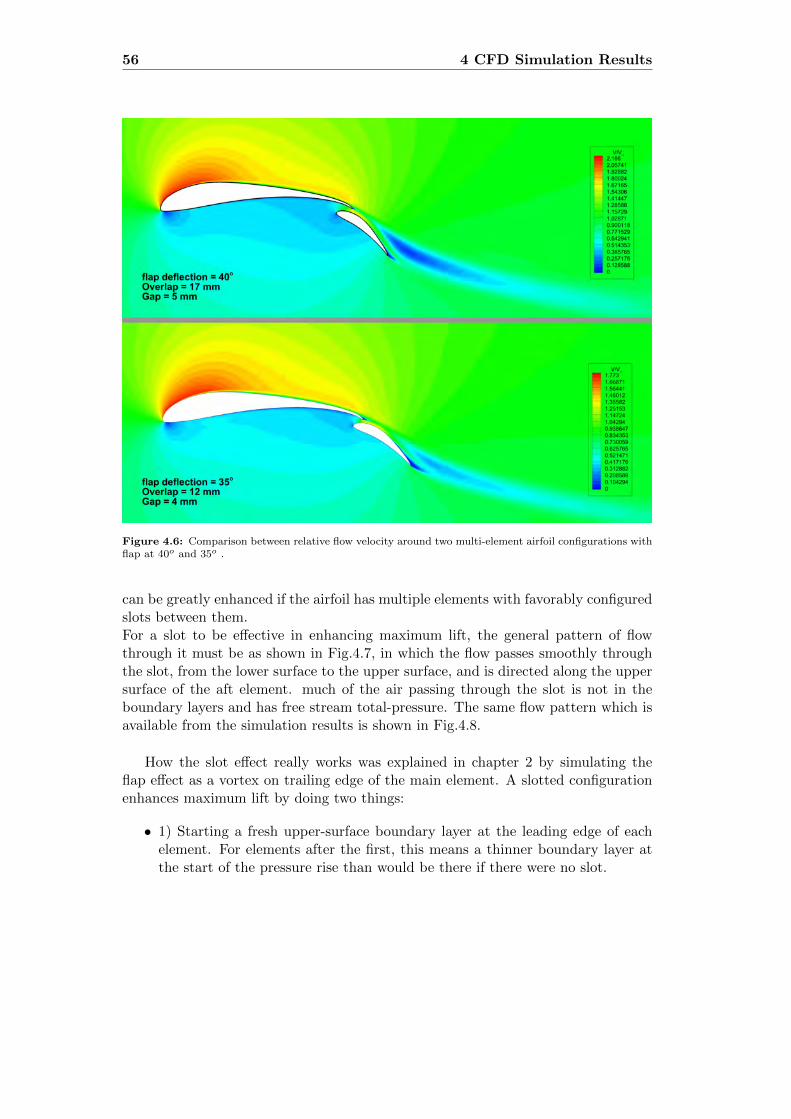
56 4 CFD Simulation Results
Figure 4.6: Comparison between relative flow velocity around two multi-element airfoil configurations withflap at 40o and 35o .
can be greatly enhanced if the airfoil has multiple elements with favorably configuredslots between them.For a slot to be effective in enhancing maximum lift, the general pattern of flowthrough it must be as shown in Fig.4.7, in which the flow passes smoothly throughthe slot, from the lower surface to the upper surface, and is directed along the uppersurface of the aft element. much of the air passing through the slot is not in theboundary layers and has free stream total-pressure. The same flow pattern which isavailable from the simulation results is shown in Fig.4.8.
How the slot effect really works was explained in chapter 2 by simulating theflap effect as a vortex on trailing edge of the main element. A slotted configurationenhances maximum lift by doing two things:
• 1) Starting a fresh upper-surface boundary layer at the leading edge of eachelement. For elements after the first, this means a thinner boundary layer atthe start of the pressure rise than would be there if there were no slot.

4.3 Discussion 57
Figure 4.7: Typical features of the flow through an effective high-lift slot.
Figure 4.8: Streamlines passing through the slot, resulted from CFD simulation in the current work showsan effective high-lift slot.
• 2) Slot can provide leading edge suction-peak suppression or trailing-edgedumping-velocity elevation. Slots do this in either of two ways, or both si-multaneously, depending on the situation of the given airfoil element.
– Leading edge suction-peak suppression: When there is an element aheadessentially by providing some flow turning ahead of the leading edge ofthe current element, so that the flow does not rush around the leadingedge as fast as it otherwise would.
– The dumping effect: In this case trailing edge of the forward element(in this project, main airfoil) is placed in a high velocity region near theleading edge of the trailing element (flap airfoil). It results in reducing thevelocity at the leading edge of an element and elevating the velocity atthe trailing edge of the main airfoil which both reduce the total velocitydrop the boundary layer is subjected to.[9] This phenomena can be seen in
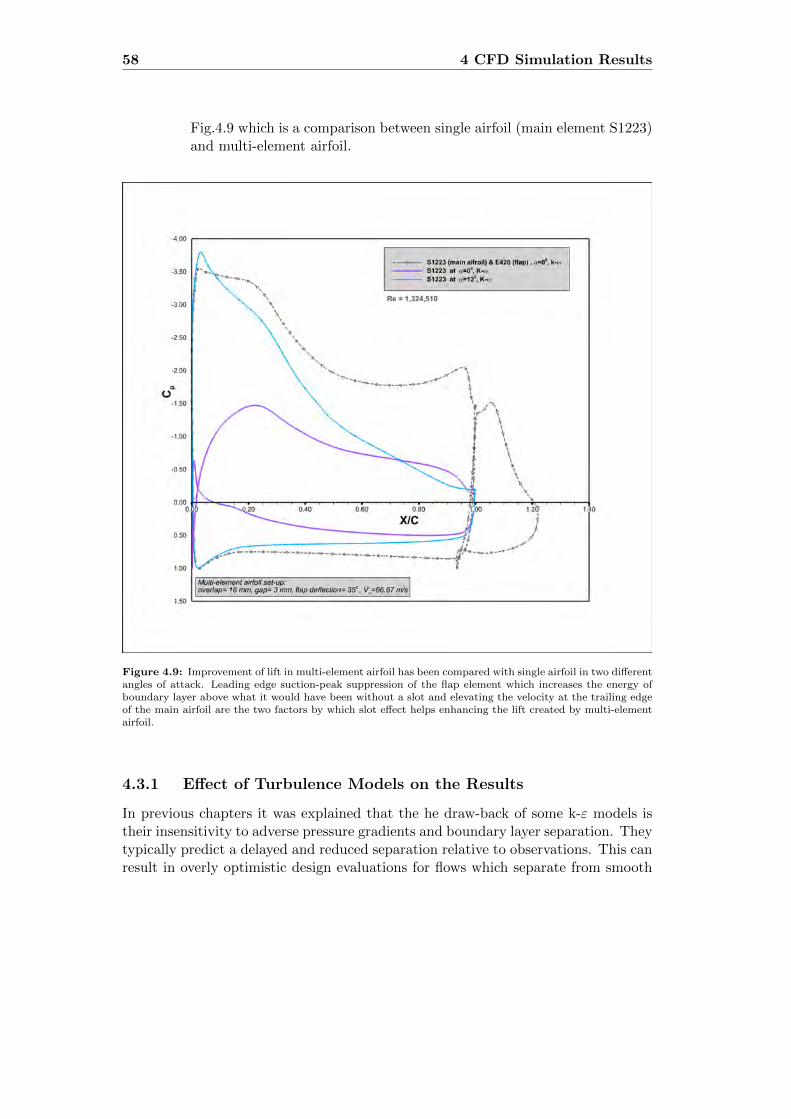
58 4 CFD Simulation Results
Fig.4.9 which is a comparison between single airfoil (main element S1223)and multi-element airfoil.
Figure 4.9: Improvement of lift in multi-element airfoil has been compared with single airfoil in two differentangles of attack. Leading edge suction-peak suppression of the flap element which increases the energy ofboundary layer above what it would have been without a slot and elevating the velocity at the trailing edgeof the main airfoil are the two factors by which slot effect helps enhancing the lift created by multi-elementairfoil.
4.3.1 Effect of Turbulence Models on the Results
In previous chapters it was explained that the he draw-back of some k-ε models istheir insensitivity to adverse pressure gradients and boundary layer separation. Theytypically predict a delayed and reduced separation relative to observations. This canresult in overly optimistic design evaluations for flows which separate from smooth

4.3 Discussion 59
surfaces. The k-ε model is therefore not widely used in external aerodynamics.[8]The SST k-ω model has been designed to avoid the freestream sensitivity of thestandard k-ω model, by combining elements of the ω-equation and the ε- equation.In addition, the SST model has been calibrated to accurately compute flow separationfrom smooth surfaces. Within the k-ω model family, it is therefore recommendedto use the SST model. The SST model is one of the most widely used modelsfor aerodynamic flows. It is typically somewhat more accurate in predicting thedetails of the wall boundary layer characteristics than the Spalart-Allmaras model.In order to investigate the difference between these models several simulations weredone. Among the models Realizable k-ε, Spalart-Allmaras and SST k-ω which wasselected as the default turbulence model for this work were used. Results of thesimulations are briefly plotted in Fig.4.10 and Fig.4.11 show the difference betweenthe resultant pressure coefficient for a specific multi-element configuration. As itcould be predicted there is a close similarity between Spalart-Allmaras and SST k-ω.The main difference between them can be visualized in critical points of the airfoilwhich are near the leading-edge and trailing-edge. Obviously realizable k-ε showsan unreliable result for the simulation.
4.3.2 Separation Bubbles
Another interesting phenomenon which may affect race car aerodynamics is a lam-inar bubble in the boundary layer. The boundary layer that starts at the airfoil’sleading edge is laminar initially but, typically, for Re > 0.2 × 10⁶ a transition toturbulent boundary layers occurs along the upper surface (suction side). On manyairfoils with relatively large upper-surface curvatures, high local curvature over theforward part of the chord may initiate a laminar separation when the airfoil is ata moderate angle of incidence. But the increased thickness of the boundary layerresults in a transition to a turbulent boundary layer, which is less sensitive to stall.Consequently, the flow reattaches, creating a bubble with an enclosed area of re-circulating flow. Small disturbances grow much more readily and at low Reynoldsnumbers in separated, as compared to attached, boundary layers. Consequently, theseparated laminar boundary layer may undergo transition to turbulence with charac-teristic rapid thickening. This thickening may be sufficient for the lower edge of thenow turbulent shear layer to come back into contact with the surface and reattach asa turbulent boundary layer on the surface. In this way, a bubble of fluid is trappedunder the separated shear layer between the separation and reattachment points.Within the bubble, the boundary of which is usually the streamline that leaves thesurface at the separation point, two regimes exist. In the upstream region, a pocketof stagnant fluid at constant pressure extends back some way; behind this, a circu-latory motion develops, as shown in Fig.4.13, with the pressure in this latter regionincreasing rapidly towards the reattachment point.
• A short bubble of the order of 1% of the chord in length that exerts negligible
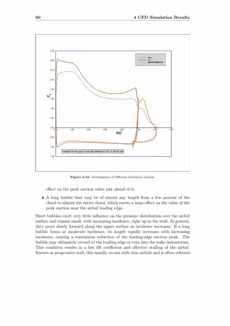
60 4 CFD Simulation Results
Figure 4.10: Investigation of different turbulence models.
effect on the peak suction value just ahead of it.
• A long bubble that may be of almost any length from a few percent of thechord to almost the entire chord, which exerts a large effect on the value of thepeak suction near the airfoil leading edge.
Short bubbles exert very little influence on the pressure distribution over the airfoilsurface and remain small, with increasing incidence, right up to the stall. In general,they move slowly forward along the upper surface as incidence increases. If a longbubble forms at moderate incidence, its length rapidly increases with increasingincidence, causing a continuous reduction of the leading-edge suction peak. Thebubble may ultimately extend to the trailing edge or even into the wake downstream.This condition results in a low lift coefficient and effective stalling of the airfoil.Known as progressive stall, this usually occurs with thin airfoils and is often referred

4.3 Discussion 61
Figure 4.11: Contours of the pressure coefficient show the different between the results of the two turbulencemodels .
Figure 4.12: Laminar separation and turbulent reattachment points.
to as thin-airfoil stall.Fig.4.13 illustrates this phenomena for 35o flap deflection while the overlap and gapare respectively 5% and 4.167% of the main element chord. It results in generation ofa big wake aft of the multi-element airfoil and a performance (CL/CD) reduction of17.33% comparing to the optimum performance point which is located at 5% overlapand 1.667% gap. Fig.4.14 is a comparison of pressure coefficient plot of these twocases.

62 4 CFD Simulation Results
Figure 4.13: Laminar bubble separation and complete separation of the boundary layer at 5% overlap and4.167% gap (top) Laminar bubble separation and reattachment of the boundary layer at 5% overlap and1.667% gap (bottom).
4.3.3 Variation of Angle of Attack and Multi-element Airfoil Per-formance
Even though a motorsports wing does not see large changes in angle of attack duringforward motion, it is necessary to have as wide an operating range as possible in orderto give the aerodynamicist and the vehicle dynamicist enough options when it comesto car setup. The rear wing is often used to balance the car after the front wing setuphas been completed to compensate for any possible undesirable characteristics of thecar endowed to it by pre-existing handling traits. Due to the very low aspect ratiosof race car wings, the primary source of drag comes from the induced componentof overall drag. Therefore the chief concern in motorsports airfoil design is not oneof profile drag reduction. Instead it is a maximization of downforce and the abilityof the designed airfoil to sustain the highest possible levels of downforce across awide range of physical and aerodynamic adversities. This way he possibility of slightchanges in direction of the upcoming air and the effect of passing cars are taking

4.3 Discussion 63
Figure 4.14: Comparison between the resultant pressure coefficient plot at (5% overlap and 4.167% gap)and t (5% overlap and 1.667% gap).
to account, at least in 2D simulation; In 3D simulation this phenomena is morecomplicated. In this project for both configurations the multi element airfoils wererotated around the leading edge of the main airfoil and the simulation was performedfor different aoa increments. The results can be seen in the table 4.5 and table 4.6.Obviously with increase in angle of incidence the drag and lift both will increase, butthis increase for lift is not continuously and in some point it starts going down andthe airfoil is losing its performance significantly. The main reason of this behavioris the same thing that happens in single element airfoils and it is the moving ofseparation point toward the leading edge of the airfoil and finally stall of the airfoil.Fig.4.15 shows the turbulent intensity counters combined by streamlines around theairfoil in αf = 40o at different aoa. the flow separating from a body carries vorticityand a deficit in total-pressure, and that downstream of the tail of the body thisvortical flow becomes the wake. Wakes take on a wide variety of forms. The wakebehind a lifting body in 3D carries strong streamwise vorticity and is called a vortexwake. Wake flow not associated with lift in 3D is referred to as a viscous wake, notbecause the rest of the flow is not viscous, but because the wake is the part that hasfelt significant direct effects of viscosity. Vortex and viscous wakes are overlappingcategories, and there is no rigorous way to assign a given wake to one or the other.

64 4 CFD Simulation Results
The total drag of a body appears as a loss of momentum and an increase of energyin the wake. The loss of momentum appears as a reduction of average flow speed,while the increase of energy is seen as violent eddying (or vorticity). The size andintensity of the wake is therefore an indication of the body s profile drag. The wakeof the multielement is growing and becomes more turbulent as the angle of attackincreases. This is the main reason of more drag force and losing the performance. Ifthe airfoil incidence is sufficiently large, separation takes place not far downstreamof the maximum suction point, and a very large wake develops. This causes such amarked redistribution of the flow over the airfoil that the large area of low pressurenear the upper-surface leading edge is seriously reduced, with the result that thelift force is also greatly reduced. This condition is referred to as stall.However aswe can see the performance of the multi element airfoil is still good and reliable.Clearly the αf = 40o configuration shows a better performance by increasing theaoa, however the αf = 35o configuration has also good downforce in different aoa.Since the αf = 35o configuration was of the most interest, more simulations wereperformed to see its behavior in larger angles of incidence. Results of these series ofsimulations will be discussed in the next section.
αf = 40o O.L=7.5% Gap=1.67%
V∞ = 66.67m/s, ReM ' 1.37× 10⁶ ,Turbulent Intensity= 1%, Turbulent Viscosity Ratio=10
αmultielement CL CD
Downforce
(N)
Drag
(N)CL/CD
0o 2.998 0.0512 2387.960 40.81 58.52
2o 3.076 0.058 2449.454 46.51 65.55
4o 3.10 0.0708 2466.180 56.29 66.29
5o 3.073 0.0755 2439.55 40.70 65.41.
Table 4.5: CFD simulation results of Multi-element airfoil with flap position at αf = 40o, in different aoawhile both airfoils are rotated around the leading edge of the main element airfoil
αf = 35o O.L=5% Gap=1.67%
V∞ = 66.67m/s, ReM ' 1.37× 10⁶ ,Turbulent Intensity= 1%, Turbulent Viscosity Ratio=10
αmultielement CL CD
Downforce
(N)
Drag
(N)CL/CD
0o 2.833 0.042 2331.16 34.42 67.73
2o 2.95 0.0478 2420.44 39.24 61.68
4o 3.025 0.055 2483.96 45.182 54.98
6o 3.054 0.0643 2506.72 52.79 47.48
8o 3.026 0.0803 2463.63 65.39 37.68.
Table 4.6: CFD simulation results of Multi-element airfoil with flap position at αf = 35o, in different aoawhile both airfoils are rotated around the leading edge of the main element airfoil

4.3 Discussion 65
4.3.4 Karman vortex street
In previous section the results of simulations of the multielement airfoil in bothconfigurations were introduced and discussed. An interesting result of increasing theangle of incidence for the αf = 35o configuration occurs at αmultielement = 10o andit is similar to what is called Karman vortex street or Von Karman vortex sheetbehind a cylinder or sphere which is a repeating pattern of swirling vortices causedby the unsteady separation of flow of a fluid around blunt bodies. The vortices aregenerated periodically on alternate sides of the horizontal axis through the wake,and in this way a row of vortices is formed. The row persists a very considerabledistance downstream. This phenomenon was first explained theoretically by VonKarman in the first decade of the twentieth century. A vortex is generated in theregion behind the separation point on one side, and a corresponding vortex on theother side breaks away from the airfoil and moves downstream in the wake. When theattached vortex reaches a particular strength, it in turn breaks away and a new vortexbegins to develop, again on the second side, and so on. The wake thus consists of aprocession of equal-strength vortices, equally spaced but alternating in sign. Duringthe formation of any single vortex while it is bound to the airfoil, an increasingcirculation exists about the airfoil and generates a transverse (lift) force. With thedevelopment of each successive vortex. That is the main reason for oscillation ofaerodynamic coefficients during the CFD simulation. This force changes sign, givingrise to an alternating transverse force on the airfoil at the same frequency as that ofthe vortex shedding. If the frequency happens to coincide with the natural frequencyof the wing s oscillation, however it may be supported, appreciable vibration mayresult.[3] As mentioned in above lines the most important signs for detection of thisbehavior in CFD are oscillation in aerodynamic coefficients and not convergence ofthe problem after the long time.
4.3.5 Effect of Variation of Sportscar Speed
Like other vehicles and even more critically, racecars have to operate in differentspeeds and as a result the rearwing must show a stable and satisfactory performancein these varying conditions. New luxury sport cars benefit from the smart comput-erized control variable rearwings however according to competition rules of GT carsusage of this type of wing is still prohibited. In this work in order to observe theperformance of the multi-element airfoil, three series of simulation were done in threedifferent speeds: 66.67m/s, 55.56m/s and 44.67m/s for the αf = 35o configurationat its optimum point . The results can be seen in table4.7. By visualizing the resultswe can understand that in spite of the proportional reduction in downforce and dragwith reduction in speed, the aerodynamic coefficients and performance of the airfoilhave remained unchanged which is a good news for this multi-element configuration.

66 4 CFD Simulation Results
αf = 35o O.L=5% Gap=1.67%
Speed(m/s) CL CD
Downforce
(N)
Drag
(N)CL/CD
66.67 2.83 0.0418 2331.1575 34.417 67.73
55.56 2.826 0.0435 1614.3364 24.85 64.96
41.67 2.80 0.04424 896.36679 14.22 63.048.
Table 4.7: CFD simulation results of Multi-element airfoil with flap position at αf = 40o, in different aoawhile both airfoils are rotated around the leading edge of the main element airfoil

4.3 Discussion 67
Figure4.15:
Vari
ati
on
of
the
an
gle
of
att
ack
forαf
=40o
mu
ltie
lem
ent
con
figu
rati
on
.
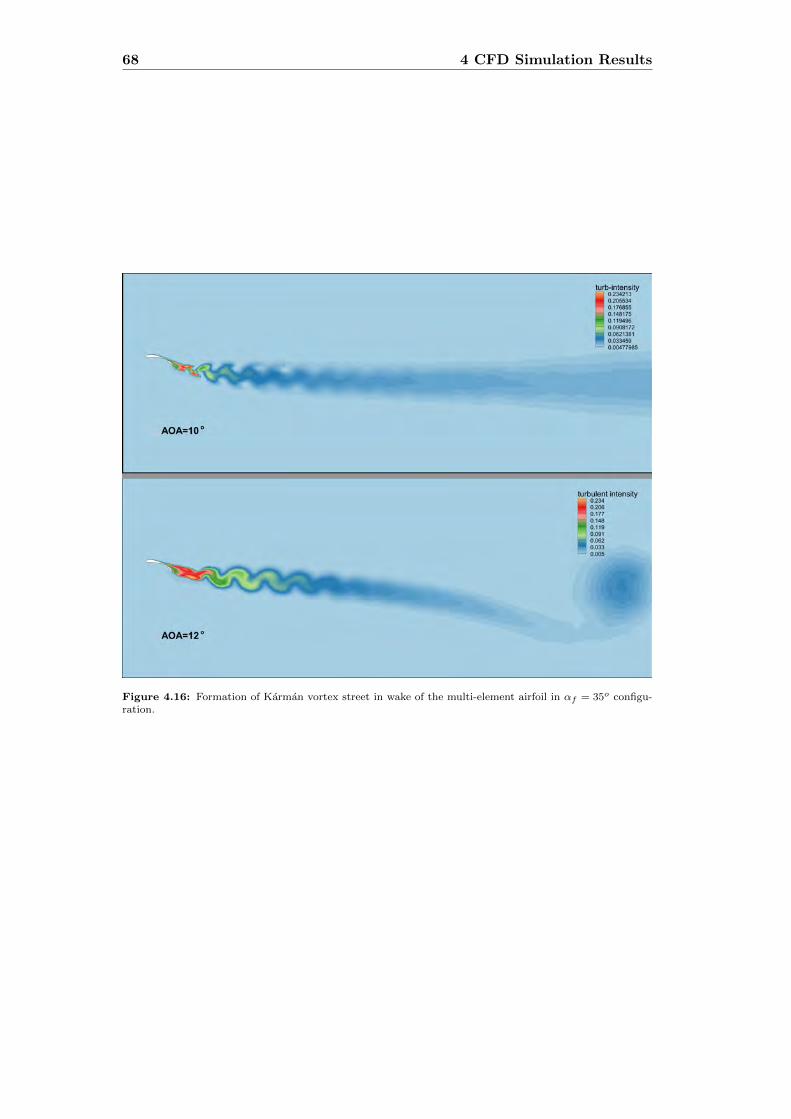
68 4 CFD Simulation Results
Figure 4.16: Formation of Karman vortex street in wake of the multi-element airfoil in αf = 35o configu-ration.
Chapter 5
Conclusions
CFD simulation of multi-element airfoils is a complicated task. The sophisticatedbehavior of flow around each airfoil and lack of ability to predict the performance ofmulti-element airfoil and the combination of different airfoils together make it evenmore harder. Even for aerodynamics, It is almost impossible to say which combina-tion of airfoils will perform better than the other before doing CFD or wind tunnelsimulations. In spite of the tremendous progress of these design tools (due to bet-ter instrumentation, communication, and computational power), the fluid dynamicphenomenon is still highly nonlinear, and predicting the effect of a particular mod-ification is not always trouble free. In this project two of the most famous high liftairfoils S1223 and E420 were used, the first one for the main element airfoil and theother one as the flap. Some geometrical modifications was performed in the trailingedge of airfoils in order to create blunt trailing edge, using XFOIL, and make thesimulation more realistic to the real airfoils. Before starting the CFD simulation inAnsys Flunet, a basic study on each single element airfoils was done in XFOIL to seehow these two airfoils, especially the main airfoil, S1223, performs in different angleof attack and different Reynolds numbers, however from the beginning of this projectwe assumed that the aoa of the main element is not going to be changed significantly.
After XFOIL simulations, the CFD simulations were performed. The main dif-ficulty in the beginning was to chose a good mesh generator software. At first wetried to used the built-in ICEM CFD in the Ansys Workbench, but lack of flexibilityof this software forced us to look for an alternative mesh generator. Finally we chosePointwise mesh generator which is a really powerful software in the market. Theabilities of this software to create hybrid meshes with a click of mouse and differentmesh examining tools designed in it, have made a unique and user-friendly meshgenerator among others.
At first CFD simulation of main element was done and the results were compared

70 5 Conclusions
to those obtained from XFOIL which were a little different since in our simulationwe considered the free stream to be completely turbulent from the beginning, Inaddition XFOIL is famous for over predicting of coefficient of lift. The main concernfor us was the type of mesh we were going to use. Obviously the best mesh couldbe a completely structured mesh, however it might be a big challenge when it comesto CFD simulation of multi-element airfoils. Changing the flap position means thewhole domain should be remeshed and if it is a structured mesh, another meaningis that working days and days to reconstruct the mesh. So finally the unstructured,triangular mesh was selected.
In the next step, CFD simulation of multi-element airfoil was done. Two con-figurations were chosen. one with flap deflection of αf = 40o and other αf = 35o.The freestream velocity was kept constant during the simulation and each flap con-figuration, gap and overlap of the flap was changed. Overlap and gap are definedaccording to O.L = ( overlap distance
main airfoil chord length)% and Gap = ( Gap distancemain airfoil chord length)%.
Each time the results were recorded and compared to the previous configuration andfinally the point, in which the best performance and enough downforce were achieved,was selected as the optimum point. The schematic of this points and distributionof their aerodynamic coefficient was plotted by automatic triangulation of the CFDdata using post-processing software Tecplot. for the αf = 40o configuration theO.L=8.25% and Gap=1.67% which creates 2375 N downforce and it performanceis 58.050 was selected as the optimum point. In the other configuration, αf = 35o
the O.L=5% and Gap=1.67% which creates 2331 N downforce and it performanceis 67.73 seemed to be the optimum point. Both configurations create great down-force and good performance. however the αf = 35o has a better performance thanαf = 40o but its generated downforce is slightly smaller. In order to be sure aboutthe accuracy of simulation, grid independence study was performed. In addition toinvestigate the behavior of multielement airfoil in different angle of attack of theupcoming freestream, several simulations were done. Fortunately the multielementis able to work perfectly in a wide range of aoa. However it might loose its perfor-mance but it still creates significant downforce. A dangerous zone for this set-up islocated at aoa = 10o and after that when the wake of the airfoil becomes to behavelike Karman vortex street which may result in vibration in the wing. However moreinvestigations should be done on this region.
As long as the rearwing should perform well in different speed and it meansdifferent Reynolnd s Numbers, two other speeds, 55.5556 m/s and 44.67 m/s, wereconsidered for the simulation. However the reduction of speed resulted in less down-force but it also caused lower drag. So in general, as it could be guessed, the changein speed does not have a significant effect on the aerodynamic coefficients and per-formance of the airfoil.
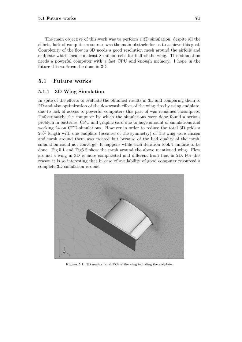
5.1 Future works 71
The main objective of this work was to perform a 3D simulation, despite all theefforts, lack of computer resources was the main obstacle for us to achieve this goal.Complexity of the flow in 3D needs a good resolution mesh around the airfoils andendplate which means at least 8 million cells for half of the wing. This simulationneeds a powerful computer with a fast CPU and enough memory. I hope in thefuture this work can be done in 3D.
5.1 Future works
5.1.1 3D Wing Simulation
In spite of the efforts to evaluate the obtained results in 3D and comparing them to2D and also optimization of the downwash effect of the wing tips by using endplate,due to lack of access to powerful computers this part of was remained incomplete.Unfortunately the computer by which the simulations were done found a seriousproblem in batteries, CPU and graphic card due to huge amount of simulations andworking 24 on CFD simulations. However in order to reduce the total 3D grids a25% length with one endplate (because of the symmetry) of the wing were chosenand mesh around them was created but because of the bad quality of the mesh,simulation could not converge. It happens while each iteration took 1 minute to bedone. Fig.5.1 and Fig5.2 show the mesh around the above mentioned wing. Flowaround a wing in 3D is more complicated and different from that in 2D. For thisreason it is so interesting that in case of availability of good computer resourced acomplete 3D simulation is done.
Figure 5.1: 3D mesh around 25% of the wing including the endplate.

72 5 Conclusions
Figure 5.2: 3D domain around 25% of the wing including the endplate.
5.1.2 Analysis of Twisted Wing
Due to the shape of the roof-line, the airflow over the center of the car will hit thewing at a steeper angle of attack than the airflow to the outer ends of the wing. Theairflow over the center of the car flows over the roof then turns downward towardsthe boot lid or trunk. The airflow to the left and right ends of the wing is at anangle closer to horizontal than the airflow to the center of the wing.
A twisted element wing allows for the varying angles of attack of the airflow ona racecar, as the air flows over the roof-line and over the sides of the car. So if astraight element wing is run at an angle of attack where you are close to the stallangle at the left and right ends of the wing, then center of the wing is seeing agreater relative angle of attack, which can prematurely stall the center of the wing.However according to the racecar aerodynamicist pioneer, Simon McBeath, what thistwist at the center of the wing also does is to reduce the wing’s downforce potentialat more moderate angles. The center section of the wing on a closed car alreadygenerates less downforce than the outer sections, because the air that encounters thecenter part of the wing has had to do some work in passing over the car’s uppersurface, and it loses energy during this passage. The wing cannot therefore developthe same magnitude of low pressure on its central underside, or indeed magnitudeof raised pressure on its central upper surface, as the relatively undisturbed air thatencounters the wing’s outer sections. In spite of this, it would be interesting to studypros and cons of twisted wing in 3D CFD environment.

Appendix A
Some Aerodynamics Definitions
This appendix presents some of the common words and expressions used in thiswork. The reason of putting them in appendix section is to reduce the amount ofunnecessary texts in the main sections of the thesis and focus on the main items, soif the reader is interested to become familiar with some theories or technical wordsmight refer to this part.
• Airfoil Geometry: If a horizontal wing is cut by a vertical plane parallel tothe centerline, the shape of the resulting section is usually like that Fig. A.2.This is an airfoil section, which for subsonic use almost always has a roundedleading edge
Figure A.1: Airfoil (wing section) geometry and definitions.
• Two-Dimensional Flow: Consider flow in two dimensions only. It is thesame as that between two planes set parallel and a little distance apart. The

74 A Some Aerodynamics Definitions
fluid can then flow in any direction between and parallel to the planes but notat right angles to them. This means that in the subsequent mathematics thereare only two space variables: x and y in Cartesian (or rectangular) coordinatesor r and θ in polar coordinates. For convenience, a unit length of the flow fieldis assumed in the z direction perpendicular to x and y. This simplifies thetreatment of two-dimensional flow problems.
• Pressure Distribution on an Airfoil: The pressure on the surface of anairfoil in flight is not uniform. Fig. shows typical pressure distributions for agiven section at various angles of attack. It is easier to deal with nondimen-sional pressure differences using p∞, the pressure far upstream, as the datum.Thus the coefficient of pressure is introduced as Looking at the sketch for zeroincidence (α = 0), we see that there are small regions at the nose and tailwhere Cp is positive but that over most of the section it is negative. At thetrailing edge the pressure coefficient comes close to +1 but does not actuallyreach it. The reduced pressure on the upper surface is tending to draw thesection upward while that on the lower surface has the opposite effect. Withthe pressure distribution as sketched, the effect on the upper surface is larger,and there is a resultant upward force on the section, that is, the lift.
Figure A.2: Typical pressure distributions on an airfoil section.
• Suction Peak: There is a decrease in pressure as we move away from thestagnation point of attachment near the leading edge, and a minimum pressurecalled the suction peak, which can be very close to the leading edge or fartherback, depending on the airfoil shape and the angle of attack. (Figure A.3)
• Pressure Recovery: The suction peak is followed by an increase in pressure,

75
or pressure recovery from the suction peak to the trailing edge.The recoveryregion is where the pressure gradient is adverse.In general, a streamlined bodywith thickness in attached flow must have a recovery region at the rear. (FigureA.3) [9]
Figure A.3: Pressure Distribution over NACA 4410 airfoil at α = 2◦
• Canonical Pressure Coefficient (Cp): In his classic Wright Brothers lec-ture on high-lift aerodynamics, Smith (1975) suggested that plotting recoverypressure distributions in what he called canonical form, in terms of a pressurecoefficient relative to the suction-peak pressure and normalized by the peakdynamic pressure, reduces the variation in ∆Cp between the suction peak andseparation and makes the separation trends easier to see. The canonical pres-sure coefficient Cp is thus defined and related to conventional Cp by:
Cp ≡P − P0
1
2ρu0
2
= 1− (ueu0
)2 = (u∞u0
)2(Cp − 1) + 1 =Cp − Cp01− Cp0
(A.1)
where the subscript o denotes conditions at the suction peak, which we willtake as the start of the recovery. Note that Cp at the suction peak is zero bydefinition, and it takes on only positive values in the recovery. Separation of aturbulent boundary layer generally occurs at Cp values between 0.4 and 0.9, amuch smaller range than we would see in terms of conventional ∆Cp.
• Rooftop: Rooftop is part of the pressure distribution of upper part of anairfoil ahead of the pressure recovery point. Rooftop pressure distribution

76 A Some Aerodynamics Definitions
have a gradually changing or approximately constant upper surface pressureover the forward part of the section.

Bibliography
[1] Joseph Katz, Race Car Aerodynamics, Designing for Speed. Bently Publishers,1995.
[2] Michael S. Selig and James J. Guglielmo, “High-lift low reynolds number airfoildesign,” journal of Aircract, vol. 34, 1997.
[3] Houghton E. L., Carpenter P. W. , Steven H. Collicott, Daniel T. Valentine,Aerodynamics for Engineering Students, 6th Edition. Elsevier, 2013.
[4] LE MANS GRAND TOURISME ENDURANCE 2014, Technical Regulations forGrand Touring Cars. FIA Sports, 2013.
[5] Liebeck, R. H., “Subsonic airfoil design,” Progress in Astronautics and Aeronau-tics: Applied Computational Aerodynamics AIAA, vol. 125, pp. 133–165, 1990.edited by P. A. Henne.
[6] van Dam, C. P., “The aerodynamic design of multi-element high-lift systems fortransport airplanes,” journal of Progress in Aerospace Sciences, vol. 38, pp. 101–144.
[7] B. Zhong , F. Scheurich, V. Titarev and D. Drikakis , “Turbulent flow simulationsaround a multi-element airfoil using URANS, DES and ILES approaches,” 19thAIAA, 22-25 June 2009.
[8] ANSYS FLUENT USER’S GUIDE, “Ansys 14.5 help.”.
[9] Doug McLean, Understanding Aerodynamics (ARGUING FROM THE REAL
PHYSICS). Wiley, 2013.