lable at ScienceDirect

Renewable Energy 87 (2016) 307e316

Contents lists avai

Renewable Energy

journal homepage: www.elsevier .com/locate/renene

A methodology for designing Francis runner blade to find minimumsediment erosion using CFD

Krishna Khanal a, *, Hari P. Neopane b, Shikhar Rai a, Manoj Thapa a, Subendu Bhatt a,Rajendra Shrestha a

a Tribhuvan University, Nepalb Kathmandu University, Nepal

a r t i c l e i n f o

Article history:Received 23 June 2015Received in revised form15 October 2015Accepted 15 October 2015Available online xxx

Keywords:Francis turbineErosionEfficiencyb-distribution

* Corresponding author.E-mail address: krishnakhanal2048@gmail.com (K

http://dx.doi.org/10.1016/j.renene.2015.10.0230960-1481/© 2015 Elsevier Ltd. All rights reserved.

a b s t r a c t

Sediment particles, especially quartz which has very high hardness factor, flowing along with watererodes turbo machinery parts such as guide vanes, runner, draft tube etc. Among them runner is verycrucial part, so its design should be optimum for minimum erosion by maintaining the highest possibleefficiency.

This paper reports on methodology for designing Francis runner blade. This involves finding bestoutlet angle (b2) and blade angle distribution (b-distribution) causing minimum possible erosion forgiven volume flow rate (Q ¼ 14.34 m3/s), head (H ¼ 40 m), rpm (N ¼ 333.33 rpm) and eroding particleflow rate (0.08 kg/s). At first, the outlet angle b2 (designing parameter) was varied from 14� to 32� usinglinear blade angle distribution for all models. Then these models were simulated to find b2. In second,with that b2, blade angle distribution was varied and simulated to find the best blade angle distributionhaving minimum erosion rate with considerable efficiency. By using hydrodynamic theory for given Qand H, main dimensions were found out and 3D model was generated using b-distribution. Relation ofdesigning parameters with erosion and efficiency was made. Optimum blade was obtained from pro-posed methodology and was compared with the reference blade in terms of erosion and efficiency.

© 2015 Elsevier Ltd. All rights reserved.

1. Introduction

The hydroelectric projects in the Himalayan range of Nepal isfacing severe silt erosion problem in turbines, which over aperiod of time significantly reduce the overall efficiency of hy-dropower. Erosion is complex process which depends upon thenumber of factors such as particle hardness, size, shape, con-centration, velocity of water, base material of turbine, etc. [1].Erosion in run-of-river is more challenging than that of reservoirtype. Rivers contain very high sediment concentration, especiallyquartz, during the monsoon season. Quartz is one of theextremely hard particle which causes mechanical wear on theturbo components due to dynamic action of particles flowingalong water [2].

Studying the dynamics of a Francis turbine has been a chal-lenging and costly job. As Francis turbine is a reaction turbine, its

. Khanal).

runner is completely dipped in water and covered by variousmechanical parts like wicket gates, guide vanes and spiral casing.This makes the visualization of the flow very difficult in therunner and very special arrangements and experimental setup isrequired to study the flow inside the Francis turbine. However,with the advent of CFD techniques the studies of the flow insidesuch complex structure have been made easy. CFD has beenwidely used in the field of turbo-machineries and hydraulicturbines. CFD tools specially for solving turbo-machineries'problems have been developed and lots of researches related tohydraulic turbines and turbo-machineries have been done withCFD.

Francis turbine is widely used in many hydropower of Nepaland some researchers have studied the erosion problem in un-derwater turbo machines and suggested the recommendation onreducing erosion. Thapa et al. summarizes the standard pro-cedures used for design of high head turbines and explained theeffect of design parameters on sediment erosion in Francis run-ner [3]. Shrestha et al. presents the alternative new way inFrancis turbine design with less erosion impact by incorporating

Nomenclature

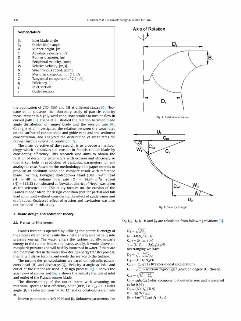
b1 Inlet blade angleb2 Outlet blade angleB Runner height, [m]C Absolute velocity, [m/s]D Runner diameter, [m]U Peripheral velocity, [m/s]W Relative velocity, [m/s]N Synchronous speed, [rpm]Cm Meridian component of C, [m/s]Cu Tangential component of C, [m/s]h Efficiency, [-]1 Inlet section2 Outlet section

Fig. 1. Axial view of runner.

Fig. 2. Velocity triangle.

K. Khanal et al. / Renewable Energy 87 (2016) 307e316308

the application of CFD, FEM and FSI at different stages [4]. Neo-pane et al. presents the laboratory study of particle velocitymeasurement in highly swirl conditions similar to turbine flow incurved path [5]. Thapa et al. studied the relation between bladeangle distribution of runner blade and the erosion rate [6].Gaungjie et al. investigated the relation between the wear rateson the surface of runner blade and guide vane and the sedimentconcentration, and analyzed the distribution of wear rates fornormal turbine operating condition [7].

The main objective of the research is to propose a method-ology which minimizes the erosion in Francis runner blade byconsidering efficiency. This research also aims to obtain therelation of designing parameters with erosion and efficiency sothat it can help in prediction of designing parameters for anyanalogous case. Based on the methodology, this paper intends topropose an optimum blade and compare result with referenceblade. For this, Devighat Hydropower Plant (DHP) with head(H) ¼ 40 m, volume flow rate (Q) ¼ 14.34 m3/s, speed(N) ¼ 333.33 rpm situated at Nuwakot district of Nepal was takenas the reference site. This study focuses on the erosion of theFrancis runner blade for design condition (not for partial and fullload condition) without considering the effect of guide vanes anddraft tubes. Coalesced effect of erosion and cavitation was alsonot included in this study.

2. Blade design and sediment theory

2.1. Francis turbine design

Francis turbine is operated by utilizing the potential energy ofthe storage water partially into the kinetic energy and partially intopressure energy. The water enters the turbine radially, impartsenergy to the runner blades and leaves axially. It works above at-mospheric pressure andwill be fully immersed inwater. If there aresediment particles in thewater flowduring energy transfer process,then it will strike turbine and erode the surface to the turbine.

The turbine design calculations are based on hydraulic param-eters head (H) and discharge (Q). Velocity triangle at inlet andoutlet of the runner are used in design process. Fig. 1 shows theaxial view of runner and Fig. 2 shows the velocity triangle at inletand outlet of the Francis runner blade.

The dimensioning of the outlet starts with assuming norotational speed at best efficiency point (BEP) i.e. Cu2 ¼ 0. Outletangle (b2) is selected from 14� to 32� and calculations were madeas:

Knownparameters are Q, N, H and b2. Unknownparameters like

D2, U2, U1, D1, B and b1 are calculated from following relations [3].

D2 ¼ffiffiffiffiffiffiffiffiffiffi4:Q

P:Cm2

qN ¼ 60.U2/(P.D2)Cm2¼U2.tan (b2)h ¼ (U1Cu1�U2Cu2)/(gH)Rearranging we have

D2 ¼ffiffiffiffiffiffiffiffiffiffiffiffiffiffiffiffiffiffiffiffiffi

240:Qp2:N:tanðb2Þ

3q

U2 ¼ (P.D2.N)/60Cm1 ¼ Cm2/1.1 (10% meridional acceleration)C1 ¼

ffiffiffiffiffiffiffiffiffiffiffiffiffiffiffiffiffiffiffiffiffiffiffiffiffiffiffiffiffiffiffiffiffiffiffiffiffiffiffiffiffiffiffiffiffiffiffiffiffiffiffiffiffiffiffið1� reaction degreeÞ:2gH

p(reaction degree 0.5 chosen)

Cu1 ¼ffiffiffiffiffiffiffiffiffiffiffiffiffiffiffiffiffiffiffiffiC21 � C2

m1

qU1 ¼ hgH/Cu1 (whirl component at outlet is zero and h assumedto be 0.96)D1 ¼ (60.U1)/(PN)B ¼ Q/(PDCm1)b1 ¼ tan�1(Cm1/(U1� Cu1))

K. Khanal et al. / Renewable Energy 87 (2016) 307e316 309

2.2. Wear mechanism and erosion model

Damages in hydro power turbines are mainly caused by cavi-tation problems, sand erosion, material defects and fatigue. Ingeneral, wear mechanisms can be classified in three categories;mechanical, chemical and thermal actions. In hydraulic turbinemechanical wear of main concern.

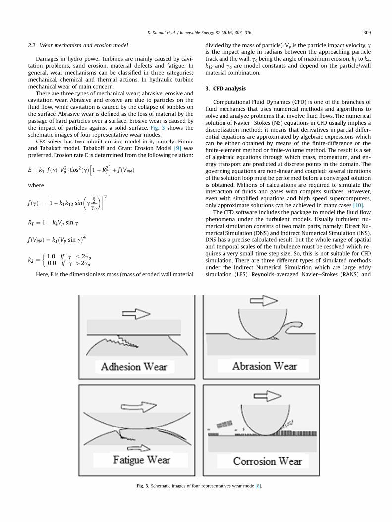
There are three types of mechanical wear; abrasive, erosive andcavitation wear. Abrasive and erosive are due to particles on thefluid flow, while cavitation is caused by the collapse of bubbles onthe surface. Abrasive wear is defined as the loss of material by thepassage of hard particles over a surface. Erosive wear is caused bythe impact of particles against a solid surface. Fig. 3 shows theschematic images of four representative wear modes.

CFX solver has two inbuilt erosion model in it, namely: Finnieand Tabakoff model. Tabakoff and Grant Erosion Model [9] waspreferred. Erosion rate E is determined from the following relation:

E ¼ k1$f ðgÞ$V2p $Cos

2ðgÞh1� R2T

iþ f ðVPNÞ

where

f ðgÞ ¼�1þ k1k12 sin

�g

p2go

��2

RT ¼ 1� k4Vp sin g

f ðVPNÞ ¼ k3�Vp sin g

�4

k2 ¼1:0 if g � 2go0:0 if g >2go

Here, E is the dimensionless mass (mass of eroded wall material

Fig. 3. Schematic images of four re

divided by the mass of particle), Vp is the particle impact velocity, gis the impact angle in radians between the approaching particletrack and the wall, go being the angle of maximum erosion, k1 to k4,k12 and go are model constants and depend on the particle/wallmaterial combination.

3. CFD analysis

Computational Fluid Dynamics (CFD) is one of the branches offluid mechanics that uses numerical methods and algorithms tosolve and analyze problems that involve fluid flows. The numericalsolution of NaviereStokes (NS) equations in CFD usually implies adiscretization method: it means that derivatives in partial differ-ential equations are approximated by algebraic expressions whichcan be either obtained by means of the finite-difference or thefinite-element method or finite-volume method. The result is a setof algebraic equations through which mass, momentum, and en-ergy transport are predicted at discrete points in the domain. Thegoverning equations are non-linear and coupled; several iterationsof the solution loopmust be performed before a converged solutionis obtained. Millions of calculations are required to simulate theinteraction of fluids and gases with complex surfaces. However,even with simplified equations and high speed supercomputers,only approximate solutions can be achieved in many cases [10].

The CFD software includes the package to model the fluid flowphenomena under the turbulent models. Usually turbulent nu-merical simulation consists of two main parts, namely: Direct Nu-merical Simulation (DNS) and Indirect Numerical Simulation (INS).DNS has a precise calculated result, but the whole range of spatialand temporal scales of the turbulence must be resolved which re-quires a very small time step size. So, this is not suitable for CFDsimulation. There are three different types of simulated methodsunder the Indirect Numerical Simulation which are large eddysimulation (LES), Reynolds-averaged NaviereStokes (RANS) and

presentatives wear mode [8].

Fig. 4. Head versus mesh elements.

Table 1Rate of erosion.

SN Test duration (min) Rate of erosion (mg/gm/min)

1 40 0.282 80 0.213 125 0.274 170 0.245 215 0.326 260 0.307 305 0.268 350 0.35Average 0.28

K. Khanal et al. / Renewable Energy 87 (2016) 307e316310

detached eddy simulation (DES). RANS is the oldest and mostcommon approach to turbulence modeling. The equation ofReynolds-averaged NaviereStokes (RANS) is defined as:

rDUi

Dt¼ vP

vXiþ v

vXj

"m

vUi

vxjþ vUj

vxi

!� ru0iu

0j

#

The left hand side of the equation describes the change in meanmomentum of fluid element and the right hand side of the equationis the assumption of mean body force and divergence stress. ru;iu

;j is

an unknown term and called Reynolds stresses. Due to the aver-aging procedure information is lost, which is then feed back intothe equations by turbulence model [9].

The shear-stress transport (SST) k-umodel [9] was developed byMenter to effectively blend the robust and accurate formulation ofthe k-u model in the near-wall region with the free-stream inde-pendence of the k-ε model in the far field. To achieve this, Baseline(BSL) k-w model, which combines advantages of Wilcox k-w and k-εmodel, is provided with the proper transport behavior to limit theover prediction of eddy viscosity. The equations are:

BSL model:

Fig: 5. (a) Test specimen before test. (b) Test specimen after 3

vðrkÞvt

þ v

vxj

�rUjk

� ¼ v

vxj

"�mþ mt

sk3

�vkvxj

#þ Pk � b

0rkuþ Pkb

vðruÞvt

þ v

vxj

�rUju

� ¼ v

vxj

"�mþ mt

su3

�vu

vxj

#

þ ð1� F1Þ2r1

su2u

vkvxj

vu

vxjþ a3

u

kPk

� b3ru2 þ Pub

The proper transport behavior can be obtained by a limiter tothe formulation of eddy-viscosity:

vt ¼ a1kmaxða1u; SF2Þ

where

vt ¼ mt=r

3.1. Mesh independent test

Since the results would be numerical approximation using CFXsolver, the numerical analysis was done to check the numericalstability and accuracy of the simulation.

Mesh independence test was done for the selection of number

50 min. (c) Result of CFD analysis d) Runner of JHC [12].

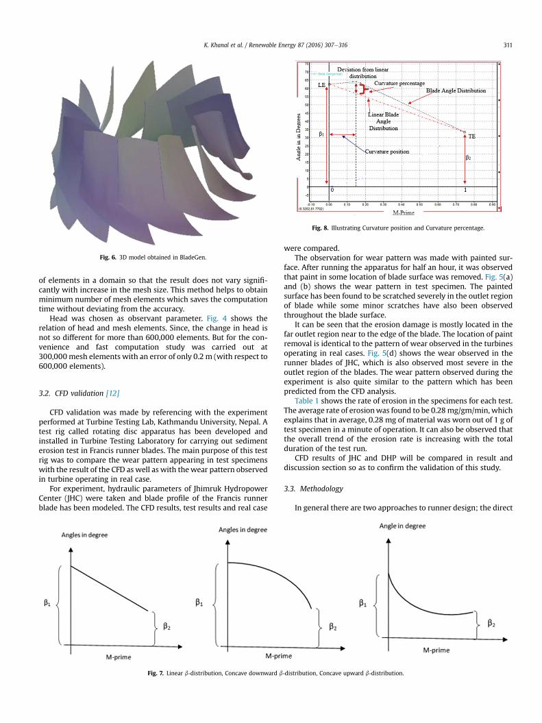
Fig. 6. 3D model obtained in BladeGen.

Fig. 8. Illustrating Curvature position and Curvature percentage.

K. Khanal et al. / Renewable Energy 87 (2016) 307e316 311

of elements in a domain so that the result does not vary signifi-cantly with increase in the mesh size. This method helps to obtainminimum number of mesh elements which saves the computationtime without deviating from the accuracy.

Head was chosen as observant parameter. Fig. 4 shows therelation of head and mesh elements. Since, the change in head isnot so different for more than 600,000 elements. But for the con-venience and fast computation study was carried out at300,000mesh elements with an error of only 0.2 m (with respect to600,000 elements).

3.2. CFD validation [12]

CFD validation was made by referencing with the experimentperformed at Turbine Testing Lab, Kathmandu University, Nepal. Atest rig called rotating disc apparatus has been developed andinstalled in Turbine Testing Laboratory for carrying out sedimenterosion test in Francis runner blades. The main purpose of this testrig was to compare the wear pattern appearing in test specimenswith the result of the CFD as well as with thewear pattern observedin turbine operating in real case.

For experiment, hydraulic parameters of Jhimruk HydropowerCenter (JHC) were taken and blade profile of the Francis runnerblade has been modeled. The CFD results, test results and real case

Fig. 7. Linear b-distribution, Concave downward b

were compared.The observation for wear pattern was made with painted sur-

face. After running the apparatus for half an hour, it was observedthat paint in some location of blade surface was removed. Fig. 5(a)and (b) shows the wear pattern in test specimen. The paintedsurface has been found to be scratched severely in the outlet regionof blade while some minor scratches have also been observedthroughout the blade surface.

It can be seen that the erosion damage is mostly located in thefar outlet region near to the edge of the blade. The location of paintremoval is identical to the pattern of wear observed in the turbinesoperating in real cases. Fig. 5(d) shows the wear observed in therunner blades of JHC, which is also observed most severe in theoutlet region of the blades. The wear pattern observed during theexperiment is also quite similar to the pattern which has beenpredicted from the CFD analysis.

Table 1 shows the rate of erosion in the specimens for each test.The average rate of erosionwas found to be 0.28mg/gm/min, whichexplains that in average, 0.28 mg of material was worn out of 1 g oftest specimen in a minute of operation. It can also be observed thatthe overall trend of the erosion rate is increasing with the totalduration of the test run.

CFD results of JHC and DHP will be compared in result anddiscussion section so as to confirm the validation of this study.

3.3. Methodology

In general there are two approaches to runner design; the direct

-distribution, Concave upward b-distribution.

K. Khanal et al. / Renewable Energy 87 (2016) 307e316312

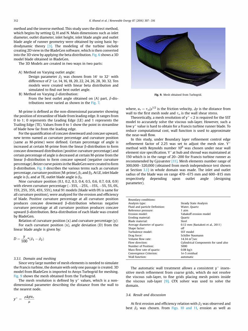
method and the inverse method. This study uses the direct method,which begins by setting Q, H and N. Main dimensions such as inletdiameter, outlet diameter, inlet height, inlet blade angle and outletblade angle of runner geometry were obtained by using basic hy-drodynamic theory [3]. The modeling of the turbine includecreating 2D view in the BladeGen software, which is then convertedinto the 3D view by applying the beta distribution. Fig. 6 shows a 3Dmodel blade obtained in BladeGen.

The 3D Models are created in two ways in two parts:

A) Method on Varying outlet angle:

Design parameter b2 was chosen from 14� to 32� withdifference of 2� i.e. 14, 16, 18, 20, 22, 24, 26, 28, 30, 32. Tenmodels were created with linear beta distribution andsimulated to find out best outlet angle.

Fig. 9. Mesh obtained from Turbogrid.

B) Method on Varying b-distribution: From the best outlet angle obtained on (A) part, b-dis-tributions were varied as shown in the Fig. 7.

Boundary conditions:Analysis type: Steady State AnalysisFluid and particle Definition: Water, QuartzReference pressure: 1 atmErosion model: Tabakoff erosion modelEroding material: QuartzBlade material: SteelAverage diameter of quartz: 0.12 mm (Bastakoti et al., 2011)Shape factor: offTurbulence model: SST modelDrag force: Schiller NaumannVolume flow rate: 14.34 m3/secFlow direction: Cylindrical Components for sand alsoNumber of Position: 5000Mass flow rate of quartz: 0.08 kg/sConvergence Criterion: 1e-5 residualWall function: automatic

M-prime is defined as the non-dimensional parameter showingthe position of streamline of blade from leading edge. It ranges from0 to 1; 0 represents the Leading Edge (LE) and 1 represents theTrailing Edge (TE). Values from 0 to 1 show the point in streamlineof blade how far from the leading edge.

For the quantification of concave downward and concave upward,new terms named as curvature percentage and curvature position(same as M-prime) were defined. Certain percentage of angle isincreased at certain M-prime from the linear b-distribution to formconcave downward distribution (positive curvature percentage) andcertain percentage of angle is decreased at certainM-prime from thelinear b-distribution to form concave upward (negative curvaturepercentage). Beizercurvepoints in theBladeGenwerecreated to formb-distribution. Fig. 8 describes the various terms such as curvaturepercentage, curvature position (M-prime),b1 andb2. At LE, inlet bladeangle is b1 and at TE, outlet blade angle is b2.

Nine curvature position (0.1, 0.2, 0.3, 0.4, 0.5, 0.6, 0.7, 0.8, 0.9)with eleven curvature percentage (�35%, �25%, �15%, �5%, 5%, 0%,15%, 25%, 35%, 45%, 55%), total 91 models (blade with 0% is same forall curvature position), were analyzed for the erosion and efficiencyof blade. Positive curvature percentage at all curvature positionproduces concave downward b-distribution whereas negativecurvature percentage at all curvature position produces concaveupward b-distribution. Beta-distribution of each blade was createdby BladeGen.

Relation of curvature position (x) and curvature percentage (y):For each curvature position (x), angle deviation (D) from the

linear blade angle is given by:

D ¼ y100

*ðb1 � b2Þ

3.3.1. Domain and meshingSince very large number of mesh elements is needed to simulate

the Francis turbine, the domainwith only one passage is created. 3Dmodel from BladeGen is imported to Ansys Turbogrid for meshing.Fig. 9 shows the mesh obtained from the Turbogrid.

The mesh resolution is defined by yþ values, which is a non-dimensional parameter describing the distance from the wall tothe nearest node.

yþ ¼ rDyutm

where, ut ¼ tu/r1/2 is the friction velocity, Dy is the distance fromwall to the first mesh node and tu is the wall shear stress.

Theoretically, a mesh resolution of yþ< 2 is required for the SSTmodel to accurately solve the viscous sub-layer. However, such alow yþ value is hard to obtain for a Francis turbine runner blade. Toreduce computational cost, wall function is used to approximatethe near-wall flow.

In this study, under Boundary layer refinement control edgerefinement factor of 2.25 was set to adjust the mesh size. Yþ

method with Reynolds number 106 was chosen under near wallelement size specification. Yþ at hub and shroud was maintained at150 which is in the range of 20e200 for Francis turbine runner asrecommended by Gjfsæster [11]. Mesh elements number range of300,000e320,000 (obtained from mesh independence test shownat Section 3.1) in whole domain was made. The inlet and outletradius of the blade was on range 470e675 mm and 600e815 mmrespectively depending upon outlet angle (designingparameter).

The automatic wall treatment allows a consistent yþ insen-sitive mesh refinement from coarse grids, which do not resolvethe viscous sub-layer, to fine grids placing mesh points insidethe viscous sub-layer [9]. CFX solver was used to solve thedomain.

3.4. Result and discussion

At first erosion and efficiency relation with b2 was observed andbest b2 was chosen. From Figs. 10 and 11, erosion as well as

Fig. 10. Erosion vs b2.

Fig. 11. Efficiency Vs b2.

Table 2Detail of runner inlet.

Position Hub Mean Shroud

Circumferential speed (m/sec) 22.2 23.64 26.08Circumferential component of the

absolute velocity (m/sec)18.7 18.7 18.7

Blade angle b1 (degree) 63.04 54.4 43.05

Table 3Detail of runner outlet without swirl.

Position Hub Mean Shroud

Circumferential speed (m/sec) 12.18 17.46 27.06Blade angle b2 (degree) 31.94 23.52 15.68

K. Khanal et al. / Renewable Energy 87 (2016) 307e316 313

efficiency of b2 ¼ 14� and b2 ¼ 16� were nearly same and were bestthan others. It can be noticed from the graph that erosion tends toincrease as outlet angle increases and efficiency tends to decreasewith increase in outlet angle with some irregularities. By consid-ering the manufacturing complexity, b2 ¼ 14� is relatively difficultto manufacture than b2 ¼ 16�. So b2 ¼ 16� was selected as best b2whose corresponding b1 ¼ 43�.

Different blade profile of selected outlet angle (b2 ¼ 16�) wasproduced and then the result was plotted. Fig. 12 shows meridionalview of Francis runner including the main dimension of the bladeused in the simulation.

Fig. 12. Meridional view of runner blade showing main dimensions of b2 ¼ 16o.

The hub and shroud curve were chosen arbitrarily and also theleading edge and trailing edge of blade were made as shown inFig. 12. Each of the stream line has different inlet blade angle b1 anddifferent outlet blade angle b2. Table 2 and Table 3 summarize theinlet and outlet blade angle at hub, mean and shroud of the blade.

All the dimension of geometry such as leading edge, trailingedge, hub, shroud, b1 and b2 were kept same but blade angle dis-tribution (b-distribution) from leading to trailing edge were varied.Such variation was done to produce 91 blade models.

91 models were simulated and their erosion and efficiencypattern was observed. Erosion was not the absolute measurementbut only the relative one. The relation of erosion and efficiency withblade profiles was obtained from these simulations. Also the opti-mum blade having minimum erosion relative to other bladeswithout compromising the efficiency was selected and was thencompared to the reference one.

Fig. 13 shows the relation between erosion and curvature per-centage for all curvature position. As maximum erosion take placeat single dot point on the blade and contribute more than 60% oftotal erosion, so, y-axis is set as total erosion minus maximumerosion and this compares the blade models effectively. The figurereveals that erosion is relatively high at �35% curvature and highervalues of curvature position also has higher erosion. For example,0.9 curvature position has highest erosion at �35%, 55% curvatures.Although there is no exact regular pattern of erosion according tocurvature percentage, it can be seen that the trend of erosion de-creases as we shift from negative curvature to zero curvature butpositive curvatures has almost same value of erosion with smallfluctuation for all curvature position. It was observed that theerosion increased with the increase of curvature towards thetrailing edge; that is at 0.9, 0.85, 0.8 have generally higher erosionthan other curvature positions.

Fig. 14 shows the representative graph for the erosion versescurvature position. The plot shows that erosion increases as thecurvature is shifted towards trailing edge. It can also be seen thatlarger area is eroded when the curvature position is shifted towardtrailing edge as the value of total minus maximum erosion is largerwhen the curvature is near trailing edge.

It is necessary to observe the efficiency of the models to deter-mine the appropriate blade for specific hydro site. Fig. 15 shows theefficiency verses curvature percentage for all curvature positions.The graph shows that efficiency at negative curvatures is almostconstant with small deviation but there is significant variation to-ward positive curvatures. Blade models with curvature positiongreater than 0.45 have regular decrease in efficiency as curvaturepercentage increases from zero but other curvature position showsome irregularity in efficiency as curvature percentage increasesfrom zero. The notable point is that the efficiency is higher attrailing edge (near 0.9 position) for negative curvature percentage

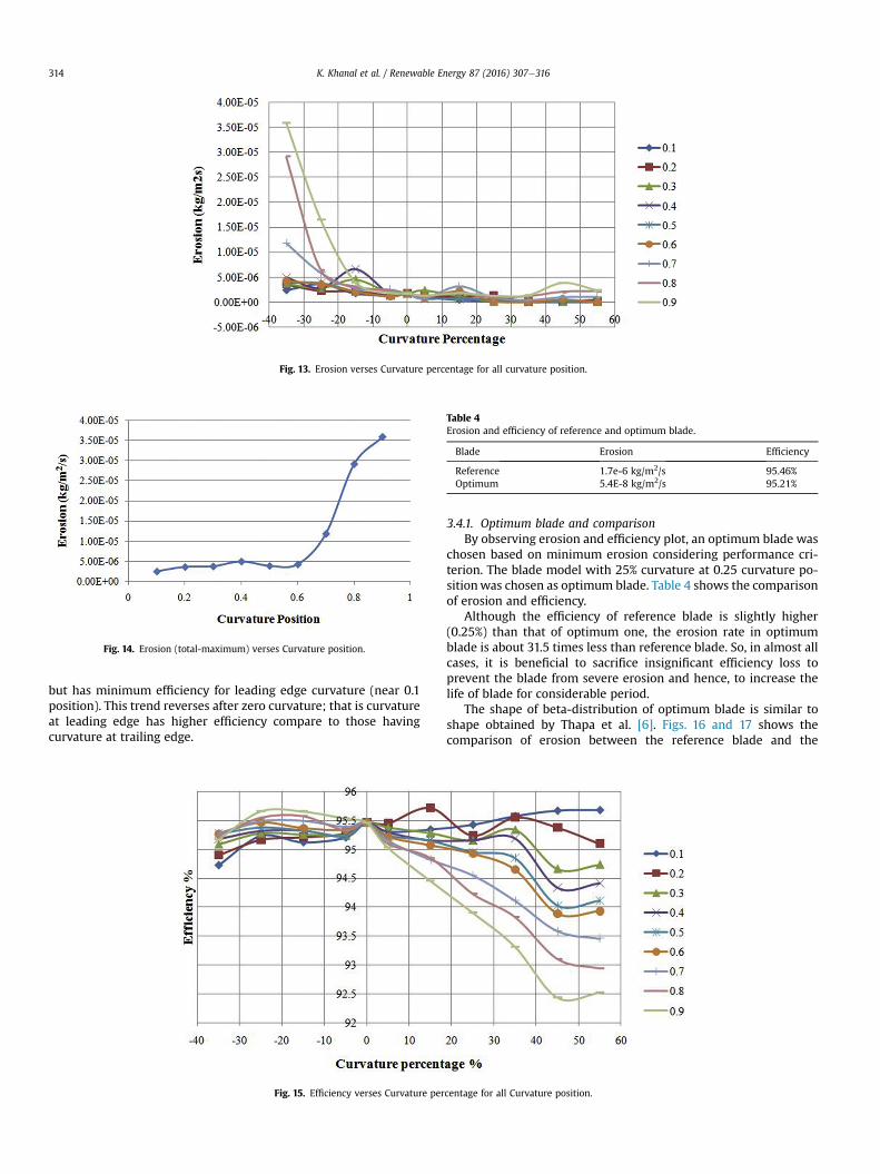
Fig. 13. Erosion verses Curvature percentage for all curvature position.

Fig. 14. Erosion (total-maximum) verses Curvature position.

Table 4Erosion and efficiency of reference and optimum blade.

Blade Erosion Efficiency

Reference 1.7e-6 kg/m2/s 95.46%Optimum 5.4E-8 kg/m2/s 95.21%

K. Khanal et al. / Renewable Energy 87 (2016) 307e316314

but has minimum efficiency for leading edge curvature (near 0.1position). This trend reverses after zero curvature; that is curvatureat leading edge has higher efficiency compare to those havingcurvature at trailing edge.

Fig. 15. Efficiency verses Curvature per

3.4.1. Optimum blade and comparisonBy observing erosion and efficiency plot, an optimum blade was

chosen based on minimum erosion considering performance cri-terion. The blade model with 25% curvature at 0.25 curvature po-sitionwas chosen as optimum blade. Table 4 shows the comparisonof erosion and efficiency.

Although the efficiency of reference blade is slightly higher(0.25%) than that of optimum one, the erosion rate in optimumblade is about 31.5 times less than reference blade. So, in almost allcases, it is beneficial to sacrifice insignificant efficiency loss toprevent the blade from severe erosion and hence, to increase thelife of blade for considerable period.

The shape of beta-distribution of optimum blade is similar toshape obtained by Thapa et al. [6]. Figs. 16 and 17 shows thecomparison of erosion between the reference blade and the

centage for all Curvature position.

Fig. 16. Erosion on the pressure and suction side of reference blade respectively.

Fig. 17. Erosion on the pressure and suction side of optimum blade respectively.

K. Khanal et al. / Renewable Energy 87 (2016) 307e316 315

optimum one respectively. Red color shows the eroded area on theblade. The figures clearly shows that erosion is significantly less inoptimized blade compare to the reference one. In optimized blade,pressure side has only some small dots of erosion and has no moreerosion in the suction side.

3.4.2. Blade profile comparisonFig. 18 shows blade profile comparison of optimum and refer-

ence blade. Red color profile is the optimized blade where as blackcolor profile is the reference blade.

Fig. 18. Blade profile comparison of optimum and reference blade.

3.4.3. Comparison of DHP and JHC [3].CFD results of this study (DHP) were compared to the referenced

JHC results.Tables 5e7 shows the comparison table of DHP blade (reference

blade) and JHC blade. Although there are some difference in theinput parameters (like shape factors, flow rate), these do notchanges the result pattern significantly. So, it can be said that therotating disc apparatus experiment performed for JHC blade can betaken as a reference material for DHP blade to confirm CFD results.

4. Conclusion and recommendation

This study has showed a methodology for designing Francisrunner blade from starting point by taking flow rate, head and rpmas designing parameter to optimized blade having minimumerosion. From the results, it is concluded that blade profile having25% curvature percentage at 0.25 curvature position is considered asoptimum blade. Although this optimized blade has 0.25% less effi-ciency than reference one, significant decrease in erosion rate hasbeen observed; numerically, erosion rate is 31.5 times less than thereference blade with considerable reduction in erosion area. Thus, ithas been proved that significant improvement can be made tominimize erosion while maintaining efficiency by changing therunner blade profile and hence, increase the life of runner blade.From the charts shown, it can also be deduced that increasing outletangle above 200, in general, increases the erosion and decreasesefficiency. Even if there are some irregularities, erosion is relativelyhigher at negative curvature (concave upward) than positive

Table 5General parameters for CFX-Pre.

Parameter DHP JHC

Turbulence SST SSTFlow state Steady SteadyFlow type Inviscid InviscidErosion model Tabakoff Tabakoff

Table 6Parameters for CFX-pre sediment data.

Data DHP JHC

Material Quartz QuartzDiameter 0.12 mm 0.1 mmShape factor Off 1Flow rate 0.08 kg/s 0.07 kg/s

Table 7Result from CFX-post erosion analysis.

Parameter DHP JHC

Sediment erosion 1.7E-6 kg/m2/s 3.0E-7 kg/m2/sEfficiency 95.46% 95.05%

K. Khanal et al. / Renewable Energy 87 (2016) 307e316316

curvature (concave downward) and curvature towards the trailingedge causes more erosion than that in the leading edge for bothnegative and positive curvatures. Also, it has been revealed that ef-ficiency would be better if the curvature is made near the leadingedge. Therefore, it can be concluded that it is better to design bladeprofile by making positive curvature near leading edges.

This methodology can be used for most of hydro-sites to find outoptimum Francis runner blade by minimizing erosion. However,even more precise study could be made by producing beta distri-bution with different shapes for each outlet angle and analysiscould be made on wide range of models to have better under-standing of erosion and efficiency pattern. Moreover, more so-phisticated experimental study could be made to validate theresults obtained from simulation so that it will be helpful to predictand then to reduce erosion effectively in practical application.

References

[1] Biraj Singh Thapa, Bhola Thapa, Ole G. Dahlhaug, Empirical Modelling ofSediment Erosion in Francis Turbines, Energy, SciVerse ScienceDirect, Kath-mandu. Nepal, 2012.

[2] Pankaj P. Gohil, R.P. Saini, Coalesced effect of cavitation and silt erosion inhydro turbinesda review, Renew. Sustain. Energy Rev. Sci. (2014). India,280e289.

[3] Biraj Singh Thapa, Mette Eltvik, Kristine Gjosaeter, Ole G. Dahlhaug,Bhola Thapa, Chiang Mai, Design optimization of francis runner for sedimenthandling, Int. J. Hydropower Dams (2012). Thailand, 1e9.

[4] Krishna Prasad Shrestha, Bhola Thapa, Ole Gunnar Dahlhaug, Hari P. Neopane,Biraj Singh Thapa, Innovative design of Francis turbine for sediment ladenwater, in: TIM International Conference, 2012. KU, Nepal.

[5] Hari Prasad Neopane, Bhola Thapa, Ole Gunnar Dahlhaug, Particle velocitymeasurement in swirl flow, laboratory studies, Kathmandu Univ. J. Sci. Eng.Technol. 8 (2012). KU, Nepal.

[6] Biraj Singh Thapa, Amod Panthee, Hari Prasad Neopane, Some application ofcomputational tools for R&D of hydraulic turbines, Renew. Nepal (2011). KU,Nepal, 1e5.

[7] Peng Guangjie, Wang Zhengwei, Xiao Yexiang, Luo Yongyao, Abrasion pre-dictions for Francis turbines based on liquidesolid two-phase fluid simula-tions, Eng. Fail. Anal. Sci. (2013). China, 327e335.

[8] Koji Kato, Koshi Adachi, Wear Mechanisms, 2001.[9] Ansys 14.5 CFX Solver Theory Guide, 2009.

[10] S. Khanna, CFD Analysis of Supercritical Airfoil over Simple Airfoil, 2011.Dehradun: s.n.

[11] Gjoaester, Kristine, Hydraulic Design of Francis Turbine Exposed to SedimentErosion, 2011. Trondheim: s.n.

[12] H.P. Neopane, B. Rajkarnikar, B.S. Thapa, Development of rotating disc appa-ratus for test of sediment-induced erosion in Francis runner blades, Wear,ScienceDirect (2013) s.l. 119e125.

Bibliography

[13] ANSYS 11.0 Turbo Grid User Guide, 2006.[14] D. Bastakoti, H.K. Karn, Cavitation and Sediment Erosion Analysis in Francis

Turbine, 2011. Khadka.[15] K.D. Naidu, Developing Silt Consciousness in the Minds of Hydro Power

Engineers' Silting Problems in Hydro Power Plants, 1999. New Delhi, India:s.n.

[16] H.P. Neopane, Sediment Erosion in Hydro Turbine, Norwegian University ofScience and Technology (NTNU), Trondheim, 2010.

[17] B. Regmi, D. Shah, A. Nepal, A Steady-state Computational Fluid Dynam-ics(CFD) Analysis of S809 Airfoil, Institute of Engineering, Tribhuwan Uni-versity, Kathmandu, Nepal, 2013. BE thesis.

[18] R.P. Saini, Kumar, Study of cavitations in hydro turbines- a review, Renew.Sustain. Energy Rev. 14 (2010).

[19] D. Sh, M. A., Optimization of GAMM Francis Turbine Runner, World Academyof Science, Engineering and Technology, 2011.

[20] D.H.M. Shrestha, Cadastre of Potential Water Power Resources of LessStudied High Mountaneous Regions with Special Reference to Nepal, Mos-cow Power Institute, USSR, 1966 s.l.

[21] K.B. Sodari, S. Pandit, R.C. Humagain, Cavitation Based Erosion Analysis inFrancis Turbine with Modelling and Simulation, Department of MechanicalEnginneering, Central Campus Pulchowk, IOE. TU, Lalitpur, Nepal, 2012.

[22] B. Thapa, Sand Erosion in Hydraulic Machinery, Norwegian University ofScience and technology, Faculty of Engineering Science and Tehnology,De-partment of Energy and Process Engineering, Trondheim, Norway, 2004. PhdThesis.

[23] Umut Aradag, et al., Hydroturbine runner design and manufacturing, Int. J.Mater. Mech. Manuf. 1 (May 2013).

[24] Hydraulic Design of Francis Turbine Exposed to Sediment Erosion, P. J. Nor-wegian University of Science and Technology, Gogstad, 2012 s.n.

[25] Kaewnai Suthep, Wongwises Somchai, Improvement of the runner design ofFrancis turbine using computational fluid dynamics. Am. J. Eng. Appl. Sci.(2011). Bankok, Thailand, 540e547, ISSN: 1941-7020.