mve165/mmg630, applied optimization lecture 2 convexity; basic

MVE165/MMG630, Applied OptimizationLecture 2

Convexity; basic feasible solutions; thesimplex method

Ann-Brith Stromberg

2012–03–15

Lecture 2 Applied Optimization

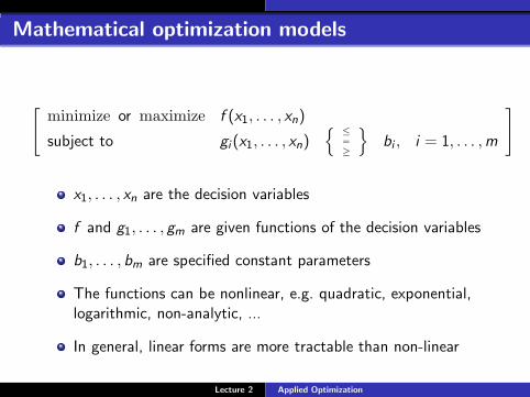
Mathematical optimization models

[

minimize or maximize f (x1, . . . , xn)

subject to gi (x1, . . . , xn){

≤

=≥

}

bi , i = 1, . . . ,m

]

x1, . . . , xn are the decision variables

f and g1, . . . , gm are given functions of the decision variables

b1, . . . , bm are specified constant parameters

The functions can be nonlinear, e.g. quadratic, exponential,logarithmic, non-analytic, ...

In general, linear forms are more tractable than non-linear


Linear optimization models (programs)

The production inventory model is a linear program (LP), i.e.,all relations are described by linear forms

A general linear program:

min or max c1x1 + . . . + cnxn

subject to ai1x1 + . . . + ainxn

{

≤

=≥

}

bi , i = 1, . . . ,m

xj ≥ 0, j = 1, . . . , n

The non-negativity constraints on xj , j = 1, . . . , n are notnecessary, but usually assumed (reformulation always possible)


Discrete/integer/binary modelling

A variable is called discrete if it can take only a countable setof values, e.g.,

Continuous variable: x ∈ [0, 8] ⇐⇒ 0 ≤ x ≤ 8Discrete variable: x ∈ {0, 4.4, 5.2, 8.0}Integer variable: x ∈ {0, 1, 4, 5, 8}

A binary variable can only take the values 0 or 1, i.e., all ornothing

E.g., a wind-mill can produce electricity only if it is built

Let y = 1 if the mill is built, otherwise y = 0Capacity of a mill: C

Production x ≤ Cy (also limited by wind force etc.)

In general, models with only continuous variables are moretractable than models with integrality/discrete requirementson the variables, but exceptions exist! More about this later.


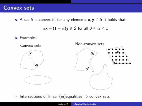
Convex sets

A set S is convex if, for any elements x, y ∈ S it holds that

αx + (1 − α)y ∈ S for all 0 ≤ α ≤ 1

Examples:

xx

x

yy

y

Convex sets Non-convex sets

⇒ Intersections of linear (in)equalities ⇒ convex sets


Convex and concave functions

A function f is convex on the set S if, for any elementsx, y ∈ S it holds that

f (αx + (1 − α)y) ≤ αf (x) + (1 − α)f (y) for all 0 ≤ α ≤ 1

A function f is concave on the set S if, for any elementsx, y ∈ S it holds that

f (αx + (1 − α)y) ≥ αf (x) + (1 − α)f (y) for all 0 ≤ α ≤ 1

⇒ Linear functions are convex (and concave)

x xy yαx + (1 − α)y αx + (1 − α)y

f (x)f (x)

f (y)

f (y)

αf (x) + (1 − α)f (y)

αf (x) + (1 − α)f (y)

f (αx + (1 − α)y)

f (αx + (1 − α)y)

Convex function Non-convex function


Global solutions of convex and linear optimizationproblem

[Theorem 11.3] Let x∗ be a local minimizer of a convex

function over a convex set. Then x∗ is also a global minimizer.

⇒ Every local optimum of a linear optimization problem is aglobal optimum

If a linear optimization problem has any optimal solutions, atleast one optimal solution is at an extreme point of thefeasible set

⇒ Search for optimal extreme point(s)

Next lecture: Linear optimization problems and the simplexmethod


A general linear program – notation

minimize or maximize c1x1 + . . . + cnxn

subject to ai1x1 + . . . + ainxn

≤=

≥

bi , i = 1, . . . , m

xj

≤ 0

unrestricted in sign

≥ 0

, j = 1, . . . , n

cj , aij , and bi are constant parameters for i = 1, . . . ,m andj = 1, . . . , n


The standard form and the simplex method forlinear programs

Every linear program can be reformulated such that:

all constraints are expressed as equalities with non-negativeright hand sidesall variables are restricted to be non-negative

Referred to as the standard form

These requirements streamline the calculations of the simplex

method

Software solvers (e.g., Cplex, GLPK, Clp) can handle alsoinequality constraints and unrestricted variables – thereformulations are made automatically


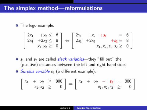
The simplex method—reformulations

The lego example:

2x1 +x2 ≤ 62x1 +2x2 ≤ 8

x1, x2 ≥ 0

⇔

2x1 +x2 +s1 = 62x1 +2x2 +s2 = 8

x1, x2, s1, s2 ≥ 0

s1 and s2 are called slack variables—they ”fill out” the(positive) distances between the left and right hand sides

Surplus variable s3 (a different example):

[

x1 + x2 ≥ 800x1, x2 ≥ 0

]

⇔

[

x1 + x2 − s3 = 800x1, x2, s3 ≥ 0

]


The simplex method—reformulations, cont.

Non-negative right hand side:

[

x1 − x2 ≤ −23x1, x2 ≥ 0

]

⇔

[

−x1 + x2 ≥ 23x1, x2 ≥ 0

]

⇔

[

−x1 + x2 − s4 = 23x1, x2, s4 ≥ 0

]

Sign-restricted (non-negative) variables:

[

x1 + x2 ≤ 10x1 ≥ 0

]

⇔

[

x1 + x12 − x2

2 ≤ 10x1, x

12 , x2

2 ≥ 0

]

⇔

[

x1 + x12 − x2

2 + s5 = 10x1, x

12 , x2

2 , s5 ≥ 0

]


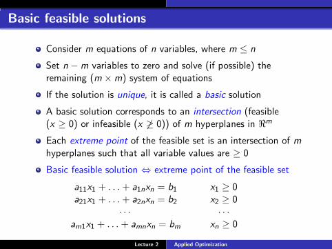
Basic feasible solutions

Consider m equations of n variables, where m ≤ n

Set n − m variables to zero and solve (if possible) theremaining (m × m) system of equations

If the solution is unique, it is called a basic solution

A basic solution corresponds to an intersection (feasible(x ≥ 0) or infeasible (x 6≥ 0)) of m hyperplanes in ℜm

Each extreme point of the feasible set is an intersection of m

hyperplanes such that all variable values are ≥ 0

Basic feasible solution ⇔ extreme point of the feasible set

a11x1 + . . . + a1nxn = b1 x1 ≥ 0a21x1 + . . . + a2nxn = b2 x2 ≥ 0

· · · · · ·am1x1 + . . . + amnxn = bm xn ≥ 0


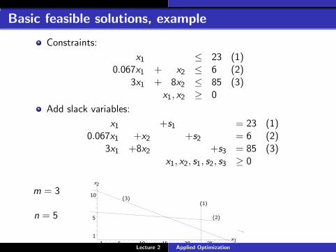
Basic feasible solutions, example

Constraints:

x1 ≤ 23 (1)0.067x1 + x2 ≤ 6 (2)

3x1 + 8x2 ≤ 85 (3)x1, x2 ≥ 0

Add slack variables:

x1 +s1 = 23 (1)0.067x1 +x2 +s2 = 6 (2)

3x1 +8x2 +s3 = 85 (3)x1, x2, s1, s2, s3 ≥ 0

x1

x2

1

1

5

5

10

10 15 20 25

n = 5

m = 3(1)

(2)

(3)


Basic and non-basic variables and solutions

basic basic solution non-basic point feasible?variables variables (0, 0)

s1, s2, s3 23 6 85 x1, x2 A yess1, s2, x1 −5 1

34 1

928 1

3s3, x2 H no

s1, s2, x2 23 −4 58

10 58

x1, s3 C nos1, x1, s3 −67 90 −185 s2, x2 I nos1, x2, s3 23 6 37 s2, x1 B yesx1, s2, s3 23 4 7

1516 s1, x2 G yes

x2, s2, s3 - - - s1, x1 - -x1, x2, s1 15 5 8 s2, s3 D yesx1, x2, s2 23 2 2 7

15s1, s3 F yes

x1, x2, s3 23 4 715

−19 1115

s1, s2 E no

x1

x2

1

1

5

5

10

10 15 20 25

A

B

C

DE

F

G HI

(1)

(2)

(3)


Basic feasible solutions correspond to solutions tothe system of equations that fulfil non-negativity

x1

x2

11

5

5

10

10 15 20 25A

B D

FG

(1)

(2)

(3)

x1 +s1 = 230.067x1 +x2 +s2 = 6

3x1 +8x2 +s3 = 85

A: x1 = x2 = 0 ⇒2

4

s1 = 23s2 = 6

s3 = 85

3

5

B: x1 = s2 = 0 ⇒2

4

s1 = 23x2 = 6

8x2 +s3 = 85

3

5

D: s3 = s2 = 0 ⇒2

4

x1 +s1 = 230.067x1 +x2 = 6

3x1 +8x2 = 85

3

5

F: s3 = s1 = 0 ⇒2

4

x1 = 230.067x1 +x2 +s2 = 6

3x1 +8x2 = 85

3

5

G: x2 = s1 = 0 ⇒2

4

x1 = 230.067x1 +s2 = 6

3x1 +s3 = 85

3

5


Basic infeasible solutions corresp. to solutions to thesystem of equations with one or more variables < 0

x1

x2

11

5

5

10

10 15 20 25

C

E

HI

(1)

(2)

(3)

x1 +s1 = 230.067x1 +x2 +s2 = 6

3x1 +8x2 +s3 = 85

H: x2 = s3 = 0 ⇒2

4

x1 +s1 = 230.067x1 +s2 = 6

3x1 = 85

3

5

C: x1 = s3 = 0 ⇒2

4

s1 = 23x2 +s2 = 6

8x2 = 85

3

5

I: s2 = x2 = 0 ⇒2

4

x1 +s1 = 230.067x1 = 6

3x1 +s3 = 85

3

5

-: s1 = x1 = 0 ⇒2

4

0 = 23x2 +s2 = 6

8x2 +s3 = 85

3

5

E: s1 = s2 = 0 ⇒2

4

x1 = 230.067x1 +x2 = 6

3x1 +8x2 +s3 = 85

3

5


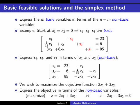
Basic feasible solutions and the simplex method

Express the m basic variables in terms of the n − m non-basic

variables

Example: Start at x1 = x2 = 0 ⇒ s1, s2, s3 are basic

x1 +s1 = 23115x1 +x2 +s2 = 63x1 +8x2 +s3 = 85

Express s1, s2, and s3 in terms of x1 and x2 (non-basic):

s1 = 23 −x1

s2 = 6 − 115x1 −x2

s3 = 85 −3x1 −8x2

We wish to maximize the objective function 2x1 + 3x2

Express the objective in terms of the non-basic variables:(maximize) z = 2x1 + 3x2 ⇔ z − 2x1 − 3x2 = 0


Basic feasible solutions and the simplex method

The first basic solution can be represented as−z +2x1 +3x2 = 0 (0)

x1 +s1 = 23 (1)115x1 + x2 + s2 = 6 (2)3x1 + 8x2 + s3 = 85 (3)

Marginal values for increasing the non-basic variables x1 andx2 from zero: 2 and 3, resp.

⇒ Choose x2 — let x2 enter the basis Draw graph!!

One basic variable (s1, s2, or s3) must leave the basis. Which?

The value of x2 can increase until some basic variable reachesthe value 0:

(2) : s2 = 6 − x2 ≥ 0 ⇒ x2 ≤ 6(3) : s3 = 85 − 8x2 ≥ 0 ⇒ x2 ≤ 105

8

}

⇒s2 = 0 when

x2 = 6(and s3 = 37)

s2 will leave the basis


Change basis through row operations

Eliminate s2 from the basis, let x2 enter the basis using rowoperations:−z +2x1 +3x2 = 0 (0)

x1 +s1 = 23 (1)115x1 +x2 +s2 = 6 (2)3x1 +8x2 +s3 = 85 (3)

−z + 95x1 −3s2 = −18 (0) −3·(2)x1 +s1 = 23 (1)−0·(2)

115x1 +x2 +s2 = 6 (2)3715x1 −8s2 +s3 = 37 (3)−8·(2)

Corresponding basic solution: s1 = 23, x2 = 6, s3 = 37.

Nonbasic variables: x1 = s2 = 0

The marginal value of x1 is 95 > 0. Let x1 enter the basis

Which one should leave? s1, x2, or s3?


Change basis ...

−z +95x1 −3s2 = −18 (0)x1 +s1 = 23 (1)

115x1 +x2 +s2 = 6 (2)3715x1 −8s2 +s3 = 37 (3)

The value of x1 can increase until some basic variable reachesthe value 0:(1) : s1 = 23 − x1 ≥ 0 ⇒ x1 ≤ 23(2) : x2 = 6 − 1

15x1 ≥ 0 ⇒ x1 ≤ 90(3) : s3 = 37 − 37

15x1 ≥ 0 ⇒ x1 ≤ 15

⇒s3 = 0 when

x1 = 15

x1 enters the basis and s3 leaves the basis

Perform row operations:−z +2.84s2 −0.73s3 = −45 (0)−(3)· 1537 ·

95

s1 +3.24s2 −0.41s3 = 8 (1)−(3) · 1537

x2 +1.22s2 −0.03s3 = 5 (2)−(3) · 1537 · 1

15x1 −3.24s2 +0.41s3 = 15 (3)·1537


Change basis ...

−z +2.84s2 −0.73s3 = −45 (0)s1 +3.24s2 −0.41s3 = 8 (1)

x2 +1.22s2 −0.03s3 = 5 (2)x1 −3.24s2 +0.41s3 = 15 (3)

Let s2 enter the basis (marginal value > 0)

The value of s2 can increase until some basic variable = 0:

(1) : s1 = 8 − 3.24s2 ≥ 0 ⇒ s2 ≤ 2.47(2) : x2 = 5 − 1.22s2 ≥ 0 ⇒ s2 ≤ 4.10(3) : x1 = 15 + 3.24s2 ≥ 0 ⇒ s2 ≥ −4.63

⇒s1 = 0 whens2 = 2.47

s2 enters the basis and s1 will leave the basis

Perform row operations:−z −0.87s1 −0.37s3 = −52 (0)−(1) · 2.84

3.240.31s1 +s2 −0.12s3 = 2.47 (1)· 1

3.24x2 −0.37s1 +0.12s3 = 2 (2)−(1) · 1.22

3.24x1 +s1 = 23 (3)+(1)


Optimal basic solution

−z −0.87s1 −0.37s3 = −520.31s1 +s2 −0.12s3 = 2.47

x2 −0.37s1 +0.12s3 = 2x1 +s1 = 23

No marginal value is positive. No improvement can be made

The optimal basis is given by s2 = 2.47, x2 = 2, and x1 = 23

Non-basic variables: s1 = s3 = 0

Optimal value: z = 52

x

y

1

1

5

5 10 15 20 25


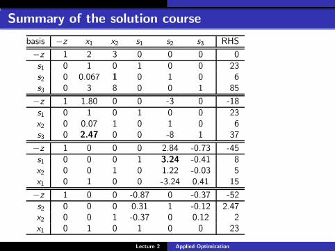
Summary of the solution course

basis −z x1 x2 s1 s2 s3 RHS

−z 1 2 3 0 0 0 0s1 0 1 0 1 0 0 23s2 0 0.067 1 0 1 0 6s3 0 3 8 0 0 1 85

−z 1 1.80 0 0 -3 0 -18s1 0 1 0 1 0 0 23x2 0 0.07 1 0 1 0 6s3 0 2.47 0 0 -8 1 37

−z 1 0 0 0 2.84 -0.73 -45s1 0 0 0 1 3.24 -0.41 8x2 0 0 1 0 1.22 -0.03 5x1 0 1 0 0 -3.24 0.41 15

−z 1 0 0 -0.87 0 -0.37 -52s2 0 0 0 0.31 1 -0.12 2.47x2 0 0 1 -0.37 0 0.12 2x1 0 1 0 1 0 0 23


Solve the lego problem using the simplex method!

maximize z = 1600x1 + 1000x2

subject to 2x1 + x2 ≤ 62x1 + 2x2 ≤ 8

x1, x2 ≥ 0

Homework!!


mve165/mmg630, applied optimization lecture 2 convexity; basic

Documents