mutual fund style drift and market conditions
TRANSCRIPT

Mutual Fund Style Drift and Market Conditions 2000 - 2015
Robert Holland, Hongyuan Wang,
Peiyi Zhang & Quentin Robert
ABSTRACT
Much work has been done on identifying style drift in mutual funds but there appears to be
a lack of evidence regarding how style drift changes as market conditions change. Using a
method which uses 12 and 24 month rolling regressions we examine R-squared values for
funds against their reported category and against the other 8 Morningstar style categories
using a range of constrains. We find that there have been significant periods of style drift
over parts of the sample period but were unable to find evidence of shift direction and could
not match many of the variations in style drift to changes in market condition. The most
significant drifts occur around the time of the 2008 financial crisis, and since this time we
show there that has been a dramatic reduction in the amount of style drift across all fund
styles. Over the whole period, funds which are core in their style appear to drift more than
other fund types. We conclude that style drift has changed over the period and that since
2008 there has been significantly less drift in mutual funds.

I Introduction
Style drift, is defined as the evolution in investment strategies over time. In the past it has been most
commonly measured by running return-based analysis to obtain resulting Style Drift Score.1 There are
many reasons why fund managers consciously diverge from stated investment strategies, one of which
is to chase outperforming rankings among their peers. In doing so, fund managers expose investors to
different risk factors than advertised, potentially impairing their ability to efficiently construct well
diversified portfolios. As we will discuss further in this paper this is a topic that has been vastly studied
in the past. However, none of the studies we have read have tried to link U.S. mutual funds style drifts
with overall market performance. For example, do mutual funds tend to drift more or less during Bearish
and Bullish market and if so what types of mutual funds drift more and where do they drift to?
Motivated by these issues, we examined the relationship between U.S. mutual funds style drift and
different market conditions based on monthly data ranging from June 2000 to December 2015. We
attempt to answer the following questions:
1. Do mutual funds’ style drift significantly during the period covered?
2. Do certain styles drift more than others?
3. Where do funds from the same category tend to drift?
4. Is there a significant relationship between market conditions and style drift?
We anticipated that certain types of funds would have a tendency of drifting more frequently during
specific market conditions. For example, Small-Cap funds were expected to drift more frequently
during Bearish markets and Large-Cap funds were expected to drift more during Bullish markets.
Furthermore, we believed that the direction of the drifts would be dictated by the specific fund’s style
within each market environment. For instance, we anticipated that a Small-Cap Growth fund would
drift to a ‘safer’ type perhaps towards Mid-Cap Core during Bearish markets and that a Mid-Cap Core
fund would drift towards a ‘riskier’ type such as Small-Cap Core during Bullish markets.
1 The Style Drift Score. By Thomas M. Idzorek and Fred Bertsch
In order to measure style drift, we conducted rolling regressions (12/24 months) on each fund against
the average monthly returns of each fund types. We identified funds that had drifted through various
conditions based around R2. We then created a market ‘index’ to measure the varying degrees of
bearishness and bullishness to link the observed style drift and market conditions.
Although we did not succeed in showing a significant link between the two, we did find a radical shift
in fund managers’ willingness to let their funds drift after the financial crisis of 2008.
II Literature Review
The importance of style drift among the investment community has increased significantly over the past
20 years and as such the amount of research has increased to meet demand for this type of analysis.
Many different sources of literature have found style drift in their studies. However, the cause of drift
is still debated among the academic community. Since the first study, a number of methods have been
used to measure the impact of various factors on style changes or ‘drift’ and the bearing they may have
on fund performance.
Many of the papers that focus on style drift have examined the movements in Style Factors (commonly
the Fama-French factors) and how a shift in these factors over time changes the sources of risk and
return for funds. Returns-based measures for measuring style changes has commonly been used since
Sharpe (1988,1992). For example, diBartolomeo & Witkowski (1997) used the returns-based method
to examine the number of funds which were misclassified. In their study, 40 percent of funds were
misclassified as a result of a poor classification system or a lack of guidelines governing managers
which allowed shifting of styles in order to increase their relative performance. Idzorek & Bertsch
(2004) expanded on this returns-based measure for finding misclassified funds by assigning ‘Style Drift
Scores’ which measure a portfolio's asset mix compared to the average asset mix, based on its volatility.
An alternative method for calculating style drift was developed by Wermers (2010) in which he uses a
‘holdings-based’ measure to assess style drift, which has the advantage of being able to track portfolios
drift when holdings are reported as well as separating active and passive drift. This distinction between
passive and active drift is derived from changes in the market capitalization of holdings, the style of the
holdings and their momentum factor. Wermers (2010) concludes that both passive and active drift
‘contribute significantly’ to total drift. Using the holdings-based method, Wermers finds that managers
who have high levels of active style drift produce superior returns. This is in contrast to Brown &
Harlow (2005), who find that funds with higher style consistency have higher returns during periods
when the benchmark is positive.
There is also widespread discussion as to the causes of style drift. According to Holmes & Faff (2008),
during 1990 and 1999, mutual funds style drifts are influenced by selectivity performances in up-market
and by flow volatility in down-market. However, the article didn’t conclude on how mutual funds may
drift investment styles in different market conditions. Fund flow has also been widely linked to style
drift. Funds both change their styles to attract new investment and change their styles as a result of new
investment (Yuhong & Wenwei, 2013). As there are often large changes in fund flows during bearish
and bullish markets, this may be cause for increased style drift in these periods (Yuhong & Wenwei,
2013). Indeed, these authors find that during bear markets, style drift increases the market timing of
funds whereas during bull markets, market timing is weakened.
Blanchett (2011) states in his paper that drifting funds see a significant increase in fund flows following
the change in Morningstar category following a returns-based style shift. Concurrently, funds tend to
drift to categories that underperform their previous category, and the drift will improve their relative
percentile ranking but remain below-average level in their new category, with no performance boost.
Despite many papers already covering style drift over significant periods, there is still no conclusive
research regarding the cause of style drift over time on U.S. mutual funds. As such, this paper will look
at the market environment throughout the last 15 years and analyze how wider market changes affect
individual fund drift. This will be done using a method of returns-based style analysis.
III Data
Creating a returns dataset for mutual funds
The data for this study came from the CSRP data set and data was collected for the period January 2000
to December 2015. The entire set of U.S mutual funds was amassed with Lipper classification names
and CUSIP IDs for each fund. Data was then filtered so only one Lipper class for each fund remained
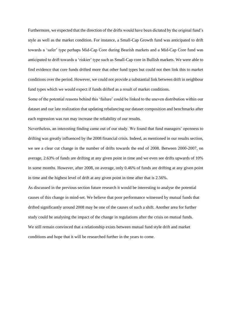
and we then removed all funds that did not have a Lipper classification that’s fits in the Morningstar

3x3 style box (Exhibit 1). These funds are categorized (and hereby called) as Large-Cap Growth (LG),
Large-Cap Core (LC), Large-Cap Value (LV), Mid-Cap Growth (MG), Mid-Cap Core (MC), Mid-Cap
Value (MV), Small-Cap Growth (SG), Small-Cap Core (SC) and Small-Cap Value (SV). There were a
total of 9,202 funds which fitted these criteria.
Monthly returns data for the same period were then gathered and the CUSIPs were matched against
those from the Lipper classification dataset. Funds were only kept where there were greater than 60
months of returns so that future analysis would be statistically significant. Other than this our data is
free of survivorship bias. This gave us a total of 1,501 funds, distributed as follows:
Table 3.1 Number of Funds by Style
Fund Type Total Number of Funds
Large-Cap Growth 266
Large-Cap Core 339
Large-Cap Value 171
Mid-Cap Growth 143
Mid-Cap Core 107
Mid-Cap Value 28
Small-Cap Growth 179
Small-Cap Core 184
Small-Cap Value 84
Total 1501
We then removed the first 6 months of data as for Mid-Cap Value there were no funds which had returns
in this period which skewed our dataset. The number of funds in each category varied over time with
the lowest total number of funds being 613 in June 2000 and the highest being 1,205 in February/March
2007. We take account for this variation in our methodology.
Creating a market type dataset
To determine market type we used daily and monthly data from the S&P 500 for the period January
2000 – December 2015. This data was retrieved from Yahoo Finance.
IV Methodology
Creating benchmarks and testing for misclassification
With the data now collected and organized we calculated the average monthly returns per fund class
and used them as benchmarks against which we ran regressions to analyse style drift. Before going
ahead and running regressions to measure drift, we checked to see whether or not some of the funds in
our dataset were misclassified as of January 2000. We did so by calculating the average of the first 12
consecutive months of returns for each benchmark and each fund as well as the standard deviation of
returns for each benchmark over that period. We defined funds as having been misclassified if their
average returns over their first 12 months were more than 1.5 standard deviations away from their
respective benchmark’s average. We found that none of the funds in the sample had been misclassified.
Deciding how to measure drift
In order to measure drift, and more specifically the instance at which the fund had drifted away from
its style, we ran rolling regressions for each fund against all benchmarks previously mentioned shifting
down by one month each time. The time period over which the regressions were run was a topic of
much discussion. Since our ultimate goal was to be able to overlap drift and market conditions (bull,
bear or neutral), we needed a time period short enough to compare with often short global market trends
but long enough to reduce the amount of noise around our results. With that in mind we ran our rolling
regressions over two distinct periods, 12 months and then 24 months. Once we ran regressions for each
funds (1501) against all benchmarks (their own and the 8 remaining), for both time periods (12 months
rolling and 24 month rolling), we turned our attention to selecting the funds that had drifted to other
styles.
Identifying periods during which funds had drifted was a pain-point for our group. We had to try a few
different methods before settling for our final one. We will now discuss each method we used and why
we ultimately did or did not pick them.
1. Betas and p-values.
We first regressed each fund against their own benchmark (using the linest function in excel), calculated
the standard deviations of the betas for each period and class type. Assuming that a fund that hadn’t
drifted would have a beta equal to or close to 1 (i.e. positively correlated with the average returns of its
own class), we identified funds that had drifted by selecting those who’s betas were significantly
different from 1 at the 10% level and who’s betas were more than 1.5 standard deviations away from 1.
In order to differentiate between drift and out/underperformance, we took the resulting funds and
regressed them against all other benchmarks. We defined funds that had drifted as those whose betas
(when regressed a second time) were between 0.9 and 1.1, i.e. had not drifted against benchmarks other
than its own.
However, after further discussion we realized that this might not be the best way to measure drift as a
fund could have a beta significantly different than 1 against its own class type if it was over or under
levered. Therefore, the results we got using this method weren’t a reliable measure of drift.
2. R2
After deliberation we opted to look at R2 as an indication of drift. The intuition behind it was that the
larger the R2, the better the model fits our data, therefore, the higher the R2 the better the benchmark
used in the regression fits the fund returns it is regressed against. For example, if a LC fund is regressed
against its own benchmark and had an R2 of 0.75 and an R2 of 0.95 when regressed against the LV
benchmark, over the same period of time, we conclude that the LC fund drifted to LV.
Within this method we decided to test two different constraints in order to differentiate between
intentional and unintentional drifts.
a. Two conditions (Two-CC)
The first test required the fund to have an R2 smaller than 0.75 when regressed against its own
benchmark and an R2 larger than 0.75 when regressed against other benchmarks. However, we often
found under this condition the same fund could have shifted towards more than one new fund type
during the same period of time. When this was the case we elected picked the class type that generated
the highest R2.
b. One condition (One CC)
This observation led us to conclude that we might not need the first condition but simply select the fund
class that generated the highest R2 when used in our regressions.
Our results section will be using the output generated from 2a. and 2b. for both 12 and 24 months rolling
regressions.
Matching periods of drift with market conditions
Once we had identified the funds that had drifted and the 12/24 months’ periods during which the drifts
had occurred, we turned our attention to matching said periods with corresponding market conditions.
This also caused the group some difficulties and we attempted various methods before settling for our
final one.
1. Dummy variable regressions
At first we attempted to regress the percentage of funds that had drifted in each period against dummy
variables Bull (1 when Bull Market, 0 otherwise), Bear (1 when Bear Market, 0 otherwise) and Neutral
(1 when Neutral Market, 0 otherwise). We defined a Bull market when the daily market value was
greater than the 200 day moving average, a Bear market when the daily market value was smaller than
the 200 day moving average and a Neutral market when there wasn’t a Bull or Bear market for 60
consecutive days.
Although our results (which we will not discuss in the next section) where significant on some of our
tests, we realized that it was practically impossible to know the exact point in time where the drift had
occurred and therefore what the true market condition was at the time of the drift. Furthermore, this
method did not take into consideration the magnitude of the Bear or Bull markets which we felt would
have a significant impact on drift. We therefore decided to discount this method.
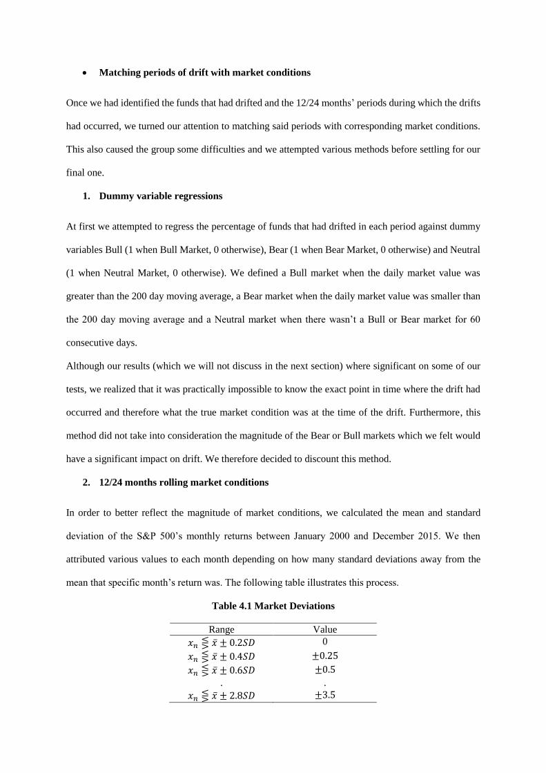
2. 12/24 months rolling market conditions
In order to better reflect the magnitude of market conditions, we calculated the mean and standard
deviation of the S&P 500’s monthly returns between January 2000 and December 2015. We then
attributed various values to each month depending on how many standard deviations away from the
mean that specific month’s return was. The following table illustrates this process.
Table 4.1 Market Deviations
Range Value
𝑥𝑛 ⋚ �̅� ± 0.2𝑆𝐷 0
𝑥𝑛 ⋚ �̅� ± 0.4𝑆𝐷 ±0.25
𝑥𝑛 ⋚ �̅� ± 0.6𝑆𝐷 ±0.5
. .
𝑥𝑛 ⋚ �̅� ± 2.8𝑆𝐷 ±3.5
By attributing more extreme values to more extreme market conditions and less extreme values to less
extreme market conditions we were able to get a more accurate representation of the market conditions.
We then calculate the 12/24 month rolling average market condition which we matched with our
previously calculated drift in graphs.
We will now discuss and interpret the results of our study.
V Results
Drift Percentage
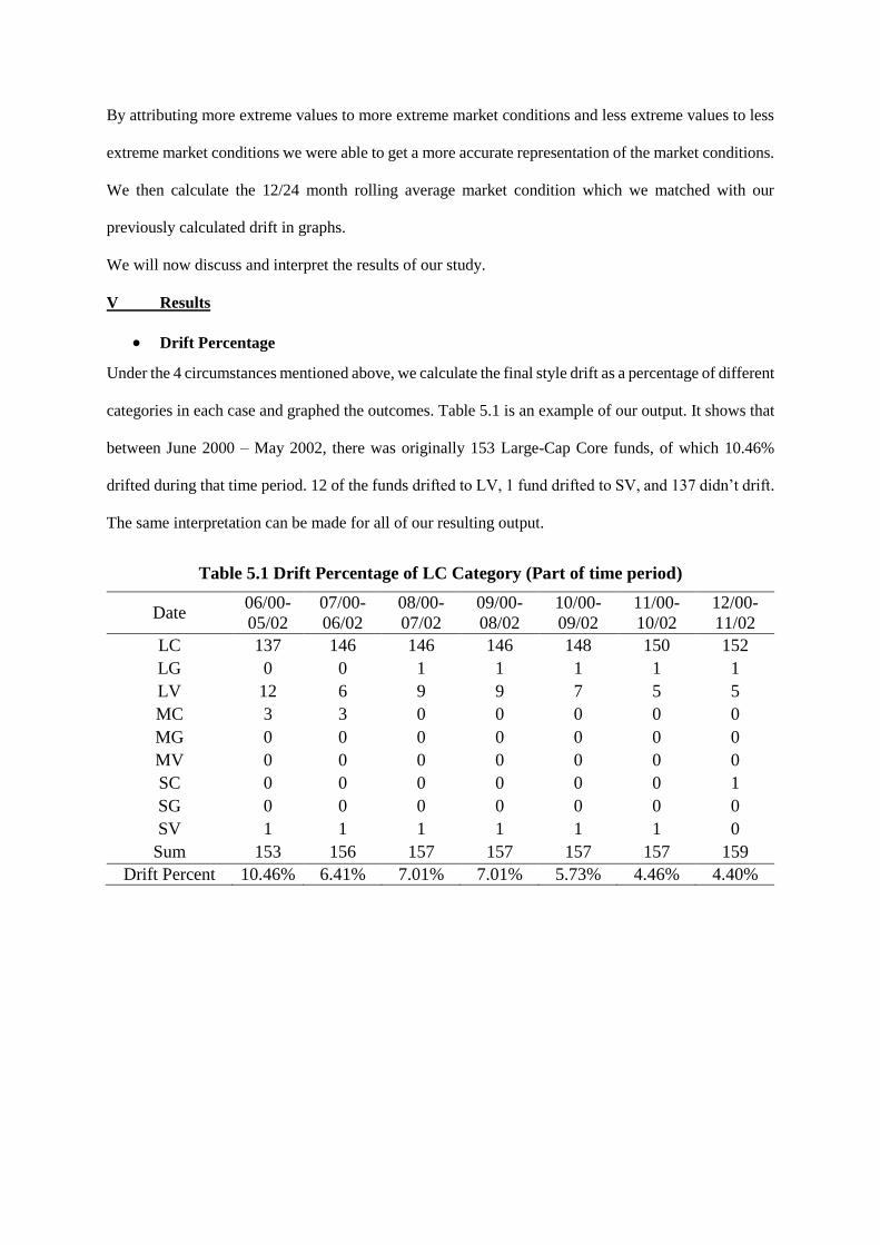
Under the 4 circumstances mentioned above, we calculate the final style drift as a percentage of different
categories in each case and graphed the outcomes. Table 5.1 is an example of our output. It shows that
between June 2000 – May 2002, there was originally 153 Large-Cap Core funds, of which 10.46%
drifted during that time period. 12 of the funds drifted to LV, 1 fund drifted to SV, and 137 didn’t drift.
The same interpretation can be made for all of our resulting output.
Table 5.1 Drift Percentage of LC Category (Part of time period)
Date 06/00-
05/02
07/00-
06/02
08/00-
07/02
09/00-
08/02
10/00-
09/02
11/00-
10/02
12/00-
11/02
LC 137 146 146 146 148 150 152
LG 0 0 1 1 1 1 1
LV 12 6 9 9 7 5 5
MC 3 3 0 0 0 0 0
MG 0 0 0 0 0 0 0
MV 0 0 0 0 0 0 0
SC 0 0 0 0 0 0 1
SG 0 0 0 0 0 0 0
SV 1 1 1 1 1 1 0
Sum 153 156 157 157 157 157 159
Drift Percent 10.46% 6.41% 7.01% 7.01% 5.73% 4.46% 4.40%
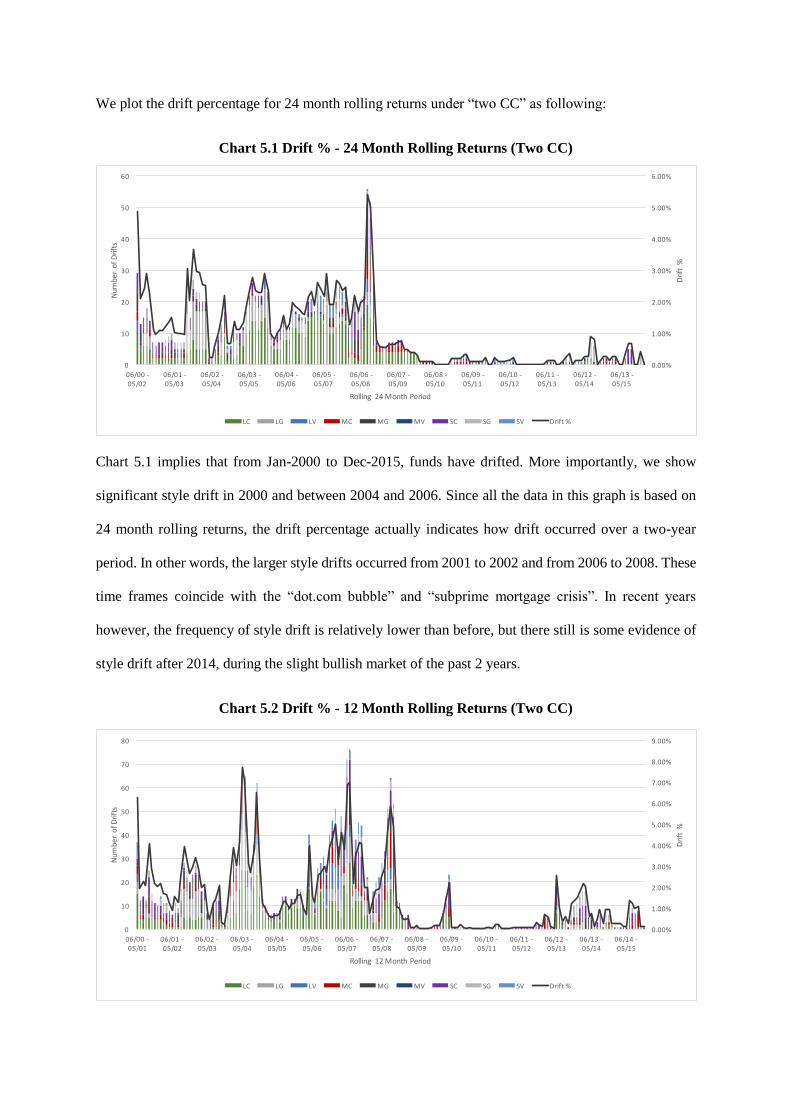
We plot the drift percentage for 24 month rolling returns under “two CC” as following:
Chart 5.1 Drift % - 24 Month Rolling Returns (Two CC)
Chart 5.1 implies that from Jan-2000 to Dec-2015, funds have drifted. More importantly, we show
significant style drift in 2000 and between 2004 and 2006. Since all the data in this graph is based on
24 month rolling returns, the drift percentage actually indicates how drift occurred over a two-year
period. In other words, the larger style drifts occurred from 2001 to 2002 and from 2006 to 2008. These
time frames coincide with the “dot.com bubble” and “subprime mortgage crisis”. In recent years
however, the frequency of style drift is relatively lower than before, but there still is some evidence of
style drift after 2014, during the slight bullish market of the past 2 years.
Chart 5.2 Drift % - 12 Month Rolling Returns (Two CC)
0.00%
1.00%
2.00%
3.00%
4.00%
5.00%
6.00%
7.00%
8.00%
9.00%
0
10
20
30
40
50
60
70
80
06/00-05/01
06/01-05/02
06/02-05/03
06/03-05/04
06/04-05/05
06/05-05/06
06/06-05/07
06/07-05/08
06/08-05/09
06/09-05/10
06/10-05/11
06/11-05/12
06/12-05/13
06/13-05/14
06/14-05/15
Drift%
Num
berofDrifts
Rolling12MonthPeriod
LC LG LV MC MG MV SC SG SV Drift%
0.00%
1.00%
2.00%
3.00%
4.00%
5.00%
6.00%
0
10
20
30
40
50
60
06/00-05/02
06/01-05/03
06/02-05/04
06/03-05/05
06/04-05/06
06/05-05/07
06/06-05/08
06/07-05/09
06/08-05/10
06/09-05/11
06/10-05/12
06/11-05/13
06/12-05/14
06/13-05/15
Drift%
NumberofDrifts
Rolling24MonthPeriod
LC LG LV MC MG MV SC SG SV Drift%
While the graph a similar pattern from that of the 24 month rolling returns, the frequency of style drift
increases slightly, which is to be expected as the regression for 12 month rolling returns contributes to
pinpoint more specifically the periods in which style drifts happened.
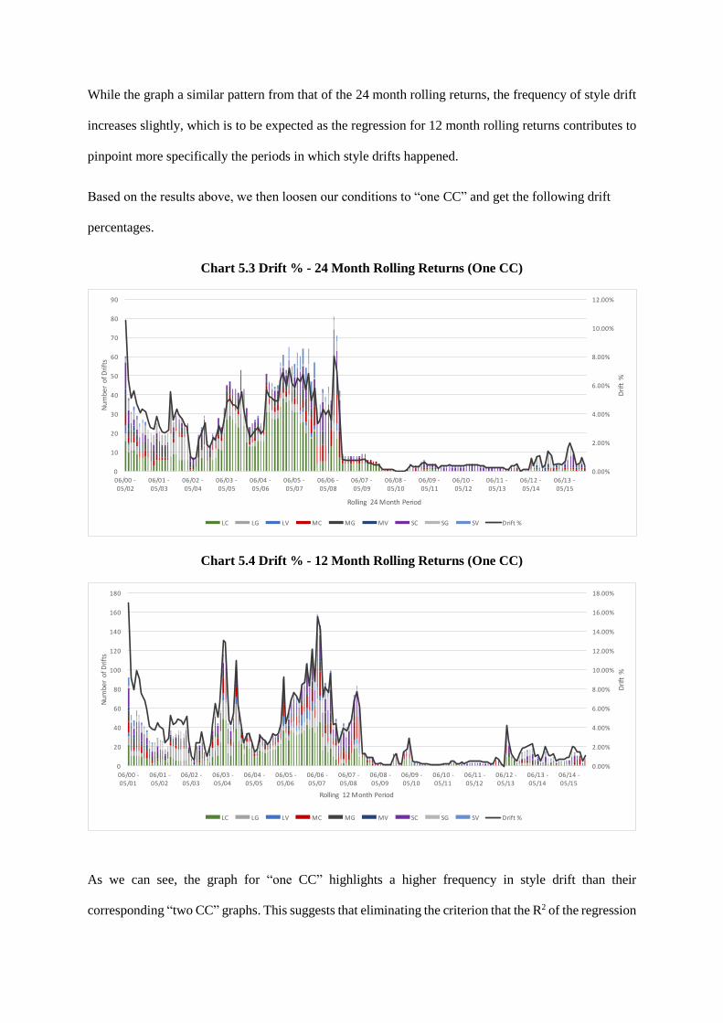
Based on the results above, we then loosen our conditions to “one CC” and get the following drift
percentages.
Chart 5.3 Drift % - 24 Month Rolling Returns (One CC)
Chart 5.4 Drift % - 12 Month Rolling Returns (One CC)
As we can see, the graph for “one CC” highlights a higher frequency in style drift than their
corresponding “two CC” graphs. This suggests that eliminating the criterion that the R2 of the regression
0.00%
2.00%
4.00%
6.00%
8.00%
10.00%
12.00%
0
10
20
30
40
50
60
70
80
90
06/00-05/02
06/01-05/03
06/02-05/04
06/03-05/05
06/04-05/06
06/05-05/07
06/06-05/08
06/07-05/09
06/08-05/10
06/09-05/11
06/10-05/12
06/11-05/13
06/12-05/14
06/13-05/15
Drift%
NumberofD
rifts
Rolling24MonthPeriod
LC LG LV MC MG MV SC SG SV Drift%
0.00%
2.00%
4.00%
6.00%
8.00%
10.00%
12.00%
14.00%
16.00%
18.00%
0
20
40
60
80
100
120
140
160
180
06/00-05/01
06/01-05/02
06/02-05/03
06/03-05/04
06/04-05/05
06/05-05/06
06/06-05/07
06/07-05/08
06/08-05/09
06/09-05/10
06/10-05/11
06/11-05/12
06/12-05/13
06/13-05/14
06/14-05/15
Drift%
NumberofDrifts
Rolling12MonthPeriod
LC LG LV MC MG MV SC SG SV Drift%
of a fund to its own category average return must be less than 0.75 increases the amount of style drift
observed.
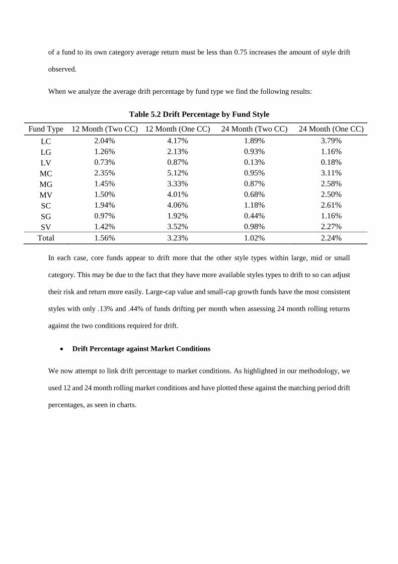
When we analyze the average drift percentage by fund type we find the following results:
Table 5.2 Drift Percentage by Fund Style
Fund Type 12 Month (Two CC) 12 Month (One CC) 24 Month (Two CC) 24 Month (One CC)
LC 2.04% 4.17% 1.89% 3.79%
LG 1.26% 2.13% 0.93% 1.16%
LV 0.73% 0.87% 0.13% 0.18%
MC 2.35% 5.12% 0.95% 3.11%
MG 1.45% 3.33% 0.87% 2.58%
MV 1.50% 4.01% 0.68% 2.50%
SC 1.94% 4.06% 1.18% 2.61%
SG 0.97% 1.92% 0.44% 1.16%
SV 1.42% 3.52% 0.98% 2.27%
Total 1.56% 3.23% 1.02% 2.24%
In each case, core funds appear to drift more that the other style types within large, mid or small
category. This may be due to the fact that they have more available styles types to drift to so can adjust
their risk and return more easily. Large-cap value and small-cap growth funds have the most consistent
styles with only .13% and .44% of funds drifting per month when assessing 24 month rolling returns
against the two conditions required for drift.
Drift Percentage against Market Conditions
We now attempt to link drift percentage to market conditions. As highlighted in our methodology, we
used 12 and 24 month rolling market conditions and have plotted these against the matching period drift
percentages, as seen in charts.

Charts 5.5 -5.8 Rolling Period Shifts against market conditions
The results appear to be distinct in some cases. Firstly, it is obvious that since 2008, there has been low
levels of drift in all of our categories. This is despite large swings in market conditions during which
we would expect to see fund managers change their styles to reflect these more bearish or bullish
markets, either seeking higher returns or safety. Prior to 2008 we see large levels of drift across time
but there appears to be very little correlation with the market type. However, it should be noted that in
each case there appears to be a large increase in style drift in the months preceding the financial crisis.
Further analysis is required to determine the nature of this shift and whether it was fund managers
seeking safety in fear of a market collapse or whether it was market confidence prompting managers to
take on additional risk and move to more aggressive investing styles.
0.00%
2.00%
4.00%
6.00%
8.00%
10.00%
12.00%
14.00%
16.00%
18.00%
-1.5
-1
-0.5
0
0.5
1
06/00-05/01
06/01-05/02
06/02-05/03
06/03-05/04
06/04-05/05
06/05-05/06
06/06-05/07
06/07-05/08
06/08-05/09
06/09-05/10
06/10-05/11
06/11-05/12
06/12-05/13
06/13-05/14
06/14-05/15
FundDrift(%)
12M
onthRollingMarketConditions
Rolling12MonthPeriod
12MonthFundDriftvMarketCondition
Rolling12monthMarketCondition Rolling12month%FundDrift(OneCC)
Drift Direction and Correlations
We then attempted to find a pattern in the direction of the drift for each fund type. We did so by
calculating the percent change of the composition of each fund type in our dataset over three year
intervals (i.e. % change of composition from June 2000 to June 2003) and over the whole period.
Table 5.3 – 12 Month Rolling Return Drift by period (% Change) (One CC)
From the tables above, we can see that the composition of our dataset change drastically over time. For
instance, if we look at the whole period there appears to be a shift towards value fund types and away
from growth. We can also see a pattern emerging where the shifts have become less distinct over the
period with the number of large percentage changes (>10%) only apparent in one fund type (MV) for
the 2012-2015 period whereas there were four significant style changes in each of the first three periods.
We have identified three possible reasons for this:
1. New funds being created in those asset classes
2. Funds in a specific class exiting the market
3. Style drift between asset classes
The way in which our study was designed does not enable us to determine which of the three has had
the most impact on the changes in fund style type over the period.
We also examined the correlation between shift percentage for each fund type.
V C G V C G
L -3.05% -6.16% -6.37% L 7.81% -21.11% 13.49%
M 119.23% 14.06% 9.55% M -16.96% 26.75% -2.97%
S 0.05% 43.47% -21.22% S 9.61% 7.87% -7.90%
V C G V C G
L 2.48% 19.21% -5.29% L 2.31% 5.57% -13.52%
M -54.67% -10.50% -6.17% M 25.79% -5.25% 2.59%
S -6.54% 12.35% -6.34% S 5.17% 4.23% -0.93%
V C G V C G
L 4.21% 2.06% -8.93% L 14.21% -4.91% -20.75%
M 68.93% -6.34% -0.93% M 75.35% 14.82% 1.36%
S 6.52% -5.34% 1.30% S 14.82% 71.54% -31.80%
2000-2015
2000-2003 2003-2006
2006-2009 2009-2012
2012-2015
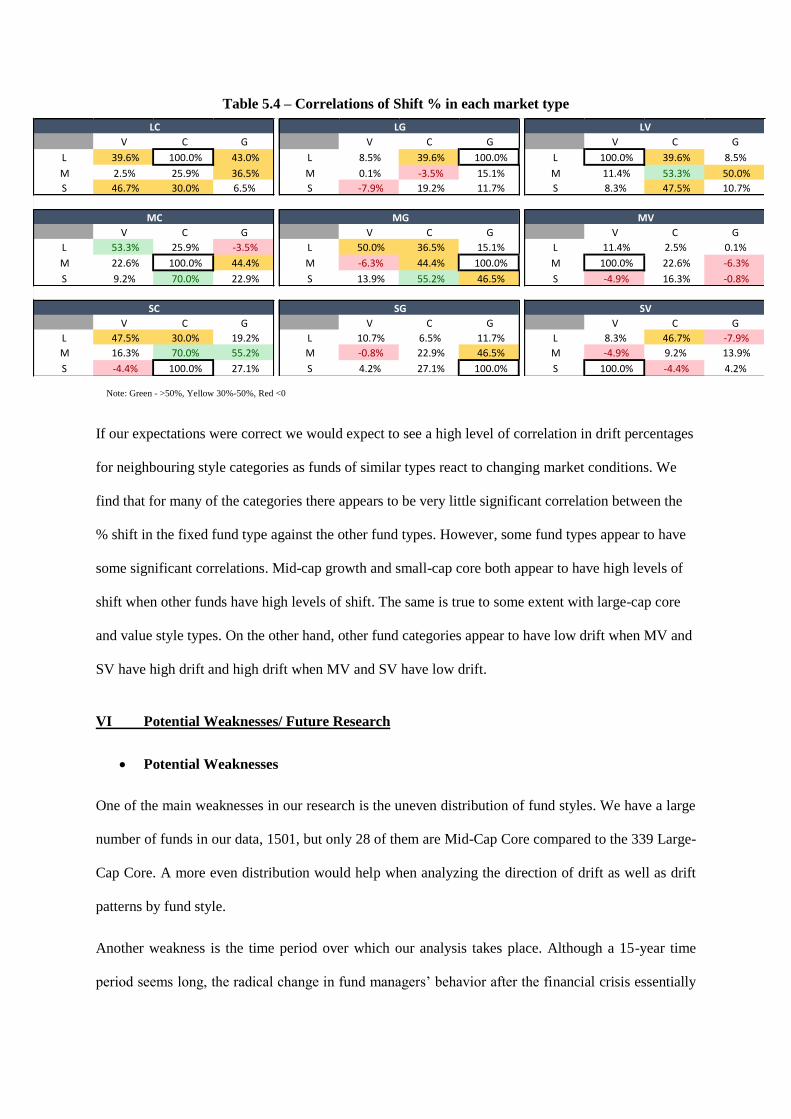
Table 5.4 – Correlations of Shift % in each market type
If our expectations were correct we would expect to see a high level of correlation in drift percentages
for neighbouring style categories as funds of similar types react to changing market conditions. We
find that for many of the categories there appears to be very little significant correlation between the
% shift in the fixed fund type against the other fund types. However, some fund types appear to have
some significant correlations. Mid-cap growth and small-cap core both appear to have high levels of
shift when other funds have high levels of shift. The same is true to some extent with large-cap core
and value style types. On the other hand, other fund categories appear to have low drift when MV and
SV have high drift and high drift when MV and SV have low drift.
VI Potential Weaknesses/ Future Research
Potential Weaknesses
One of the main weaknesses in our research is the uneven distribution of fund styles. We have a large
number of funds in our data, 1501, but only 28 of them are Mid-Cap Core compared to the 339 Large-
Cap Core. A more even distribution would help when analyzing the direction of drift as well as drift
patterns by fund style.
Another weakness is the time period over which our analysis takes place. Although a 15-year time
period seems long, the radical change in fund managers’ behavior after the financial crisis essentially
V C G V C G V C G
L 39.6% 100.0% 43.0% L 8.5% 39.6% 100.0% L 100.0% 39.6% 8.5%
M 2.5% 25.9% 36.5% M 0.1% -3.5% 15.1% M 11.4% 53.3% 50.0%
S 46.7% 30.0% 6.5% S -7.9% 19.2% 11.7% S 8.3% 47.5% 10.7%
V C G V C G V C G
L 53.3% 25.9% -3.5% L 50.0% 36.5% 15.1% L 11.4% 2.5% 0.1%
M 22.6% 100.0% 44.4% M -6.3% 44.4% 100.0% M 100.0% 22.6% -6.3%
S 9.2% 70.0% 22.9% S 13.9% 55.2% 46.5% S -4.9% 16.3% -0.8%
V C G V C G V C G
L 47.5% 30.0% 19.2% L 10.7% 6.5% 11.7% L 8.3% 46.7% -7.9%
M 16.3% 70.0% 55.2% M -0.8% 22.9% 46.5% M -4.9% 9.2% 13.9%
S -4.4% 100.0% 27.1% S 4.2% 27.1% 100.0% S 100.0% -4.4% 4.2%
SVSGSC
LC LG LV
MC MG MV
Note: Green - >50%, Yellow 30%-50%, Red <0
means that we have two separate time periods, one ranging from 2000-2008 and one ranging from 2009-
2015. Neither of these time frames are truly long enough for us to determine a strong pattern in drift.
Our results would have been significantly different had we spanned back to the early 1990s.
Furthermore, we failed to update the benchmarks for each fund style as funds drifted. This slightly
skewed our data in regards to determine the direction of style drift. If we had had more time we would
go back and adjust the composition of each fund class as we moved along.
Future Research
As we have shown in the results section, we have found a significant change in fund managers’
behaviors in regards to fund drift. This could be explained a number of ways. For instance, this could
be due to the fact that the funds that drifted before the financial crisis tended to underperform those that
didn’t. This realization might have increased their discipline in maintain a consistent style in order to
avoid the negative impact of style drift on their performance. Furthermore, since the financial crisis
regulations imposed on mutual funds have increased significantly. The majority of these regulatory
changes have targeted the disclosure of the funds holding as well as risk/returns profile. This increase
in transparency makes fund managers more accountable to current investors as well as highlights their
inconsistencies to potential investors. It could be interesting to explore the impact of these changes of
regulations on fund style drift.
VII Conclusion
In this paper we set-out to establish a clear link between market conditions and style drift. In order to
do so we started by observing and measuring style drift in 1501 U.S. mutual funds between January
2000 and December 2015.
Our initial hypothesis was that certain types of funds would have a tendency of drifting more frequently
during specific market conditions. For example, Small-Cap funds were expected to drift more in Bearish
markets and Large-Cap funds were expected to drift more in Bullish markets. Although we found that
a significant amount of funds drifted across all styles at various points in time, we were unable to show
any significant increase in fund drift during specific market conditions.
Furthermore, we expected that the direction of the drifts would have been dictated by the original fund’s
style as well as the market condition. For instance, a Small-Cap Growth fund was anticipated to drift
towards a ‘safer’ type perhaps Mid-Cap Core during Bearish markets and a Mid-Cap Core fund was
anticipated to drift towards a ‘riskier’ type such as Small-Cap core in Bullish markets. We were able to
find evidence that core funds drifted more that other fund types but could not then link this to market
conditions over the period. However, we could not provide a substantial link between drift in neighbour
fund types which we would expect if funds drifted as a result of market conditions.
Some of the potential reasons behind this ‘failure’ could be linked to the uneven distribution within our
dataset and our late realization that updating rebalancing our dataset composition and benchmarks after
each regression was run may increase the reliability of our results.
Nevertheless, an interesting finding came out of our study. We found that fund managers’ openness to
drifting was greatly influenced by the 2008 financial crisis. Indeed, as mentioned in our results section,
we see a clear cut change in the number of drifts towards the end of 2008. Between 2000-2007, on
average, 2.63% of funds are drifting at any given point in time and we even see drifts upwards of 10%
in some months. However, after 2008, on average, only 0.46% of funds are drifting at any given point
in time and the highest level of drift at any given point in time after that is 2.56%.
As discussed in the previous section future research it would be interesting to analyse the potential
causes of this change in mind-set. We believe that poor performance witnessed by mutual funds that
drifted significantly around 2008 may be one of the causes of such a shift. Another area for further
study could be analysing the impact of the change in regulations after the crisis on mutual funds.
We still remain convinced that a relationship exists between mutual fund style drift and market
conditions and hope that it will be researched further in the years to come.
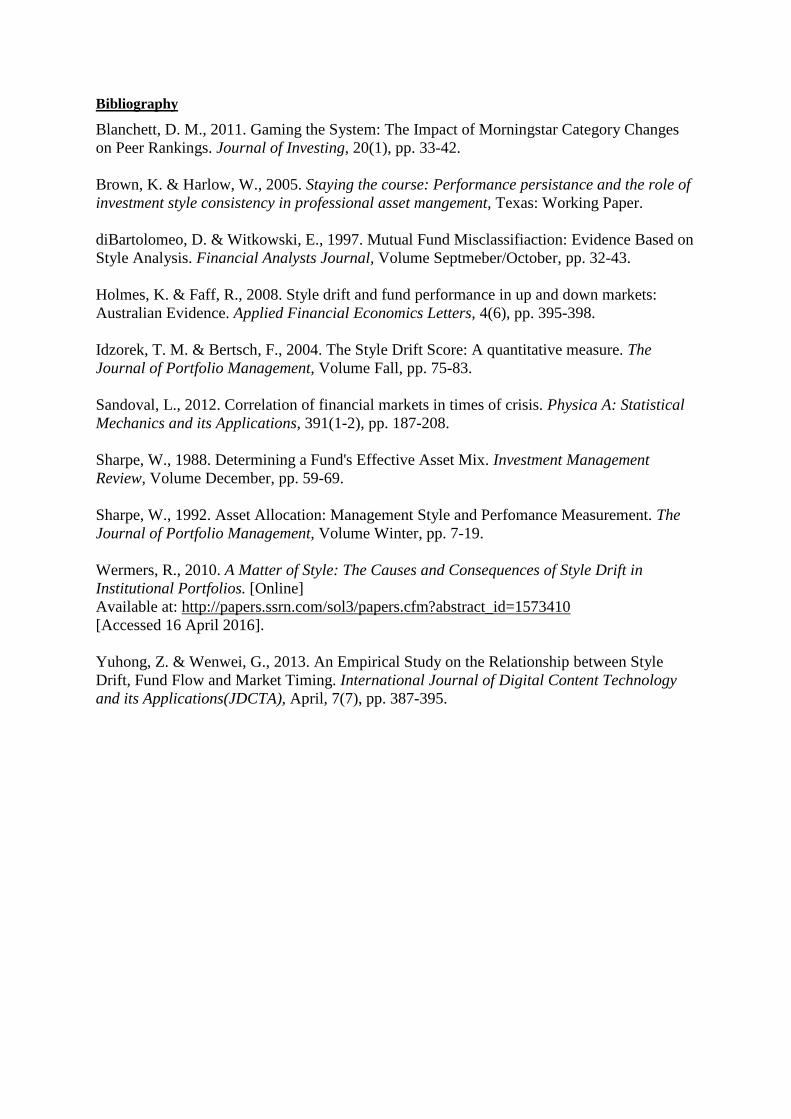
Bibliography
Blanchett, D. M., 2011. Gaming the System: The Impact of Morningstar Category Changes
on Peer Rankings. Journal of Investing, 20(1), pp. 33-42.
Brown, K. & Harlow, W., 2005. Staying the course: Performance persistance and the role of
investment style consistency in professional asset mangement, Texas: Working Paper.
diBartolomeo, D. & Witkowski, E., 1997. Mutual Fund Misclassifiaction: Evidence Based on
Style Analysis. Financial Analysts Journal, Volume Septmeber/October, pp. 32-43.
Holmes, K. & Faff, R., 2008. Style drift and fund performance in up and down markets:
Australian Evidence. Applied Financial Economics Letters, 4(6), pp. 395-398.
Idzorek, T. M. & Bertsch, F., 2004. The Style Drift Score: A quantitative measure. The
Journal of Portfolio Management, Volume Fall, pp. 75-83.
Sandoval, L., 2012. Correlation of financial markets in times of crisis. Physica A: Statistical
Mechanics and its Applications, 391(1-2), pp. 187-208.
Sharpe, W., 1988. Determining a Fund's Effective Asset Mix. Investment Management
Review, Volume December, pp. 59-69.
Sharpe, W., 1992. Asset Allocation: Management Style and Perfomance Measurement. The
Journal of Portfolio Management, Volume Winter, pp. 7-19.
Wermers, R., 2010. A Matter of Style: The Causes and Consequences of Style Drift in
Institutional Portfolios. [Online]
Available at: http://papers.ssrn.com/sol3/papers.cfm?abstract_id=1573410
[Accessed 16 April 2016].
Yuhong, Z. & Wenwei, G., 2013. An Empirical Study on the Relationship between Style
Drift, Fund Flow and Market Timing. International Journal of Digital Content Technology
and its Applications(JDCTA), April, 7(7), pp. 387-395.
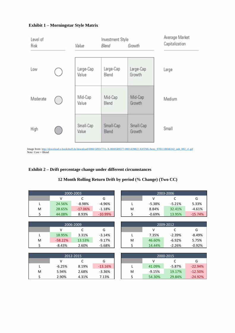
Exhibit 2 – Drift percentage change under different circumstances
12 Month Rolling Return Drift by period (% Change) (Two CC)
V C G V C G
L 24.56% -8.98% -4.96% L -5.38% -5.21% 5.33%
M 28.65% -17.06% -1.18% M 8.84% 32.41% -4.61%
S 44.08% 8.93% -10.99% S -0.69% 13.95% -15.74%
V C G V C G
L 18.95% 3.31% -3.14% L 7.35% -2.39% -8.49%
M -58.22% 13.53% -9.17% M 46.60% -6.92% 5.75%
S -8.43% 2.60% -5.68% S 14.44% -2.26% -0.92%
V C G V C G
L -6.25% 8.19% -13.16% L 41.09% -5.87% -22.94%
M 5.94% 2.68% -3.36% M -9.15% 19.17% -12.50%
S 2.90% 4.31% 7.13% S 54.30% 29.84% -24.92%
2000-2015
2000-2003 2003-2006
2006-2009 2009-2012
2012-2015
Exhibit 1 – Morningstar Style Matrix
Image from: http://download.e-bookshelf.de/download/0000/5893/77/L-X-0000589377-0001439822.XHTML/benz_9781118046142_oeb_002_r1.gif
Note: Core = Blend
24 Month Rolling Return Drift by period (% Change) (One CC)
24 Month Rolling Return Drift by period (% Change) (Two CC)
V C G V C G
L 17.05% -6.16% -10.51% L 8.66% -9.48% 10.95%
M 10.27% 13.51% 6.54% M -36.30% 17.50% -12.66%
S 0.50% 17.56% -10.09% S 17.21% 21.00% -21.28%
V C G V C G
L 15.50% 0.00% -4.38% L 1.75% 1.60% -10.39%
M -21.56% 7.31% -0.35% M 24.91% -8.60% 3.67%
S -10.27% -2.89% -1.86% S 11.76% 3.63% 0.66%
V C G V C G
L -2.02% 7.31% -12.89% L 46.44% -7.38% -25.89%
M 10.56% 1.35% -2.76% M -23.90% 32.57% -6.52%
S -0.28% 1.68% 6.57% S 17.81% 45.54% -25.50%
2012-2015
2000-2003 2003-2006
2006-2009 2009-2012
2012-2015
V C G V C G
L 20.01% -12.61% -8.11% L -2.15% -3.42% 11.48%
M 28.65% 11.62% 5.82% M -28.13% 13.73% -10.90%
S -14.77% 32.43% -6.84% S 20.19% 18.10% -23.15%
V C G V C G
L 14.65% 0.86% -4.83% L 1.08% 2.09% -10.39%
M -30.88% 12.74% 1.51% M 15.99% -16.22% 3.67%
S -17.45% -0.31% -1.86% S 22.72% 4.40% 0.66%
V C G V C G
L -1.12% 7.31% -12.89% L 34.55% -6.74% -23.90%
M 10.56% 8.55% -2.76% M -18.05% 30.16% -3.51%
S -7.21% 0.69% 6.57% S -3.71% 63.90% -24.64%
2000-2015
2000-2003 2003-2006
2006-2009 2009-2012
2012-2015