muscle force estimation in clinical gait analysisusir.salford.ac.uk/id/eprint/39257/1/muscle force...

MUSCLE FORCE ESTIMATION IN

CLINICAL GAIT ANALYSIS

Ursula Kathinka Trinler

Ph.D. Thesis

2016

MUSCLE FORCE ESTIMATION IN

CLINICAL GAIT ANALYSIS

Ursula Kathinka Trinler

School of Health Science

University of Salford, Salford, UK

2016

Submitted in Partial Fulfilment of the Requirements of the Degree of

Doctor of Philosophy, March 2016.

[i]

Table of Contents

TABLE OF CONTENTS ....................................................................................................................... I

LIST OF FIGURES ............................................................................................................................ VI

LIST OF TABLES .............................................................................................................................XII

LIST OF EQUATIONS ................................................................................................................... XIV

CONFERENCES AND WORKSHOPS ........................................................................................... XV

ACKNOWLEDGEMENTS ............................................................................................................. XVI

DECLARATION ................................................................................................................................VII

ABSTRACT ...................................................................................................................................... VIII

CHAPTER I

1 OVERVIEW ...................................................................................................................................1

1.1 INTRODUCTION ................................................................................................................ 1

1.2 THESIS OUTLINE .............................................................................................................. 4

CHAPTER II

2 BACKGROUND INFORMATION AND MAIN OBJECTIVES ..............................................7

2.1 CLINICAL SIGNIFICANCE OF MUSCULOSKELETAL ANALYSIS IN MOVEMENT SCIENCE.. 7

2.2 FUNCTIONAL ANATOMY AND PHYSIOLOGY OF THE MUSCLE TISSUE ............................ 9

2.3 DEVELOPMENT OF THE CLASSICAL GAIT ANALYSIS .................................................... 13

2.4 CLASSICAL GAIT ANALYSIS AND MUSCLE FORCE ........................................................ 15

2.5 ELECTROMYOGRAPHY AND MUSCLE FORCE ................................................................ 17

2.6 MODELLING AND SIMULATION ..................................................................................... 18

2.6.1 Musculoskeletal Models ............................................................................................ 18

2.6.2 Mathematical Models: Inverse and Forward Dynamics ........................................... 22

2.6.3 Development and Limitations of Models and Simulations ........................................ 23

[ii]

2.6.3.1 Validation Process for Musculoskeletal Modelling and Simulations ............................... 25

2.7 STATEMENT OF THE PROBLEM ...................................................................................... 27

2.8 RESEARCH QUESTION .................................................................................................... 28

CHAPTER III

3 SYSTEMATIC REVIEW OF MUSCLE FORCE ESTIMATION IN GAIT ANALYSIS ....30

3.1 INTRODUCTION INTO SYSTEMATIC REVIEWS IN MOVEMENT SCIENCE ........................ 32

3.2 METHODS ...................................................................................................................... 35

3.2.1 Literature Search ....................................................................................................... 35

3.2.1.1 Search Strategy ................................................................................................................. 35

3.2.1.2 Selection Criteria .............................................................................................................. 36

3.2.1.3 Search Process .................................................................................................................. 38

3.2.2 Quality Assessment Tool ........................................................................................... 38

3.2.3 Data Synthesis and Analysis ..................................................................................... 41

3.3 RESULTS ........................................................................................................................ 43

3.3.1 Quality Appraisal of Included Studies ....................................................................... 45

3.3.2 Measurement Equipment and Data Processing ........................................................ 49

3.3.3 Biomechanical Models .............................................................................................. 53

3.3.4 Musculoskeletal Models ............................................................................................ 53

3.3.5 Sources of Geometric Parameters ............................................................................. 55

3.3.6 Mathematical Modelling Techniques ........................................................................ 56

3.3.7 Validation of Estimated Muscle Forces .................................................................... 57

3.3.8 Outcome Measures .................................................................................................... 58

3.3.8.1 Digitalisation of Joint Moments ....................................................................................... 59

3.3.8.2 Digitalisation of Muscle Forces ........................................................................................ 67

3.4 DISCUSSION ................................................................................................................... 84

3.4.1 Joint Moments and Muscle Force Profiles ................................................................ 85

3.4.1.1 Influences on the Output through the Experimental Protocol and Data............................ 86

3.4.1.2 Influences on the Output through Modelling and Simulation Processes .......................... 88

[iii]

3.4.1.3 Muscle Force Estimation Compared to Experimental EMG ............................................ 90

3.4.1.4 Recommendations for a Protocol Suitable for the Clinical Gait Analysis ........................ 92

3.4.2 Limitations ................................................................................................................. 93

3.5 CONCLUSION ................................................................................................................. 95

CHAPTER IV

4 TECHNICAL DEVELOPMENT OF THE MODELLING AND SIMULATION

PROTOCOL .........................................................................................................................................97

4.1 INTRODUCTION TO OPENSIM ......................................................................................... 99

4.2 MUSCULOSKELETAL MODEL GAIT2392 ...................................................................... 101

4.2.1 Muscle-tendon Properties ....................................................................................... 105

4.2.2 Limitations of the Model ......................................................................................... 108

4.2.3 Adjustments to Model gait2392 ............................................................................... 108

4.3 EXPERIMENTAL DATA PREPARATION ......................................................................... 110

4.4 PIPELINE SIMTRACK .................................................................................................... 112

4.4.1 Step 1: Scaling in SimTrack .................................................................................... 113

4.4.2 Step 2: Inverse Kinematics in SimTrack .................................................................. 122

4.4.3 Complementary Step: Inverse Dynamics ................................................................ 124

4.4.4 Step 3a: Static Optimisation in SimTrack ............................................................... 125

4.4.5 Step 3b: Residual Reduction Algorithm in SimTrack .............................................. 126

4.4.6 Step 3c: Computed Muscle Control in SimTrack .................................................... 128

4.4.7 Final Structure of the OpenSim Pipeline for the Experimental Study ..................... 131

CHAPTER V

5 EXPERIMENTAL IMPLICATION OF A STANDARDISED PROTOCOL TO

ESTIMATE MUSCLE FORCES FOR ROUTINE CLINICAL GAIT ANALYSIS ...................133

5.1 INTRODUCTION ............................................................................................................ 133

5.2 METHODS .................................................................................................................... 136

5.2.1 Participants ............................................................................................................. 136

[iv]

5.2.2 Laboratory Set-up and Calibration ......................................................................... 136

5.2.3 Participant Preparation .......................................................................................... 139

5.2.4 Data Collection ....................................................................................................... 139

5.2.5 Data processing ....................................................................................................... 140

5.2.6 Data Analysis .......................................................................................................... 142

5.3 RESULTS ...................................................................................................................... 143

5.3.1 Scaling ..................................................................................................................... 144

5.3.2 Inverse Kinematics .................................................................................................. 146

5.3.3 Joint Moments ......................................................................................................... 150

5.3.4 Muscle Activations/Excitations and Force Estimations .......................................... 152

5.3.4.1 Results of the Residual Reduction Algorithm ................................................................ 152

5.3.4.2 Results of Estimated Muscle Excitations and Activations Compared to EMG .............. 157

5.3.4.3 Results of Estimated Muscle Forces compared to Estimated Activations/Excitations ... 180

5.4 DISCUSSION ................................................................................................................. 199

5.4.1 Discussion of Scaling, Joint Angles and Joint Moments ......................................... 199

5.4.2 Discussion of the Pre-Step Residual Reduction Algorithm ..................................... 201

5.4.3 Estimations of Static Optimisation vs Computed Muscle Control .......................... 202

5.4.4 Mathematical Models vs Experimental Surface EMG ............................................ 204

5.4.5 Concerning Issues with Processing Steps of SimTrack ........................................... 206

5.4.6 Limitations ............................................................................................................... 208

5.5 CONCLUSION ............................................................................................................... 210

CHAPTER VI

6 OVERALL CONCLUSION AND FUTURE WORK .............................................................212

6.1 SUMMARY OF THE THESIS’ FINDINGS ACCORDING TO THE RESEARCH QUESTIONS ... 212

6.2 CRITICAL APPRAISAL OF RESEARCH DESIGN.............................................................. 217

6.3 ORIGINAL CONTRIBUTIONS AND WIDER IMPACT ....................................................... 219

6.4 FUTURE WORK ............................................................................................................ 222

[v]

APPENDICIES ...................................................................................................................................224

A.1 OPENSIM: MUSCLE-TENDON ACTUATORS OF MODEL GAIT2392 ................................... 225

A.2 OPENSIM: MASS AND INERTIA OF GAIT2392 SEGMENTS ................................................ 226

A.3 A TYPICAL .OSIM FILE FORMAT FOR MUSCULOSKELETAL MODELS IN OPENSIM ......... 227

A.4 DEVELOPED VICON BODYLANGUAGE MODEL TO CALCULATE ANATOMICAL LANDMARKS

AND JOINT CENTRES. ................................................................................................................ 232

A.5 TECHNICAL DEVELOPMENT OF THE SCALING IN OPENSIM ............................................ 236

A.6 ETHICAL APPROVAL ....................................................................................................... 242

A.7 PARTICIPANT INFORMATION SHEET ............................................................................... 243

A.8 RESEARCH PARTICIPANT CONSENT FORM ..................................................................... 246

A.9 RESULTS OF CORRECTING THE FORCE PLATE TO THE CAMERA SYSTEM ....................... 247

LIST OF REFERENCES ..................................................................................................................250

[vi]

List of Figures

Figure 1.1. Thesis map of this work, structured in six main chapters. ....................................... 6

Figure 2.1. Illustration of a skeletal muscle with its sub-structures (Herzog, 1998). ................. 9

Figure 2.2. Muscle-tendon architecture and the relation of muscle fibres and attached tendons

adapted from Zajac (1989). ...................................................................................................... 10

Figure 2.3. Innervation of the muscle through a motor neuron with its origin in the spinal cord,

and ending with motor end plates in the muscle fibres (Lieber, 2010). ................................... 11

Figure 2.4. Schematic illustration of the electromechanical delay and its four main stages. ... 12

Figure 2.5. Photograph showing a participant equipped with reflecting markers which were

exposed to an interrupted light flashing 20 times per second (Murray et al., 1964). ............... 13

Figure 2.6. Progression of the ground reaction force vector during normal gait in stance phase

(Chris Kirtley, 2006). ............................................................................................................... 15

Figure 2.7. Different representation of muscles.. ..................................................................... 19

Figure 2.8. Force-length curve adapted from Hill (1952), and force-sarcomeres length

relationship from Lieber (2010). .............................................................................................. 21

Figure 2.9: The force-velocity relation of muscle fibres adapted from Zajac (Zajac, 1989). .. 22

Figure 2.10. Schematic flow chart of inverse (A) and forward dynamics (B), adapted from

Erdemir et al. (2007). ................................................................................................................ 23

Figure 3.1. Keywords used for the systematic database search arranged in three categories

GAIT, METHODS, and VARIABLES. ................................................................................... 36

Figure 3.2: Items used for the quality assessment tool. ............................................................ 40

Figure 3.3. Flow chart describing the process of the systematic review. Red arrows indicate

exclusion, green arrows inclusion of papers. ............................................................................ 44

Figure 3.4. Mean joint moment profiles extracted from each identified study. ....................... 61

Figure 3.5. Overall mean and one and two standard deviation bands of the hip joint moments

throughout a gait cycle, normalised to the body mass and –height. ......................................... 64

[vii]

Figure 3.6. Overall mean and one and two standard deviation bands of the knee joint moments


Figure 3.7. Overall mean and one and two standard deviation bands of the ankle joint moments


Figure 3.8. Single muscle force profiles normalised to the body mass (N/kg), extracted out of

identified studies. ...................................................................................................................... 69

Figure 3.9. Overall mean and one and two standard deviation bands of the tibialis anterior

throughout a gait cycle, normalised to the body mass, divided up into three mathematical

models static optimisation., EMG-driven, and forward dynamics. .......................................... 73

Figure 3.10. Overall mean and one and two standard deviation bands of the soleus throughout

a gait cycle, normalised to the body mass, divided up into three mathematical models static

optimisation., EMG-driven, and forward dynamics. ................................................................ 74

Figure 3.11. Overall mean and one and two standard deviation bands of the gastrocnemius



Figure 3.12. Overall mean and one and two standard deviation bands of the hamstrings



Figure 3.13. Overall mean and one and two standard deviation bands of the rectus femoris



Figure 3.14. Overall mean and one and two standard deviation bands of the vastii throughout a

gait cycle, normalised to the body mass, divided up into three mathematical models static

optimisation., EMG-driven, and forward dynamics. ................................................................ 80

Figure 3.15. Overall mean and one and two standard deviation bands of the iliopsoas (top),

gluteus maximus (mid),and gluteus medius (rear) throughout a gait cycle, normalised to the

body mass, divided up into three mathematical models static optimisation., EMG-driven, and

forward dynamics. .................................................................................................................... 83

Figure 4.1. OpenSim’s musculoskeletal model gait2392, with twelve segments, 23 degrees of

freedom and 92 muscle-tendon actuators. .............................................................................. 102

[viii]

Figure 4.2. Representation of the gluteus maximus in the OpenSim model gait2392. .......... 103

Figure 4.3. Coordinate frames and centre of mass for each segment of the gait2392 model in

OpenSim. ................................................................................................................................ 104

Figure 4.4. Graphical presentation of the Hill-type muscle tendon model adapted from Thelen

et al. (2003). ............................................................................................................................ 106

Figure 4.5. a) Gaussian curve showing a muscle force-length relationship, normalised to the

maximal isometric force of the muscle and the optimal fibre length; b) Muscle force-velocity

relationship, a describing the activation of the muscle; c) Tendon force-strain relationship;

adapted from Thelen (2003) who refers to Zajac (1989). ....................................................... 107

Figure 4.6. Subtalar and MTP joint of the foot here in the swing phase of the gait cycle (left)

and at initial contact (right) during the estimation of muscle forces with CMC are out of the

physiological boundaries. ....................................................................................................... 109

Figure 4.7. OpenSim’ standard marker model. ...................................................................... 111

Figure 4.8. SimTrack pipeline from OpenSim, adapted from Delp and colleagues (Delp et al.,

1990). ...................................................................................................................................... 112

Figure 4.9. Standard OpenSim model (left) and adjustments on the marker model to account for

placement errors. .................................................................................................................... 118

Figure 4.10. Schematic presentation of the CMC pipeline, adapted from Thelen and Anderson

(2006). .................................................................................................................................... 128

Figure 4.11. Estimated tibialis anterior muscle forces with CMC for five normal walking trials

of a typical participant while keeping the standard settings by 0.01 seconds per time step (above)

and changing the time steps to 0.005 seconds (below). ......................................................... 131

Figure 5.1. Set-up of the movement laboratory at the University of Salford showing four force

plates implemented into a ten meter long walkway, including the origin of the global reference

system (red dot), surrounded by ten infra-red cameras. ......................................................... 137

Figure 5.2. Principle of the CalTester..................................................................................... 138

Figure 5.3. Mean and one standard deviation bars representing the scaling factors of the bony

segments of the generic musculoskeletal model gait2392 in all three directions anterior-

posterior (A-P), medial-lateral (M-L), and proximal-distal (P-D). Blue indicates the primary

axis, green both other axes. .................................................................................................... 145

[ix]

Figure 5.4. Mean and one standard deviation of joint angles calculated in OpenSim (red) and

Vicon Nexus (blue) for five right walking trials of one typical participant (P02) during self-

selected walking speed. .......................................................................................................... 148

Figure 5.5. Average joint angles across five right and five left walking trials of all ten

participants during self-selected walking speed. .................................................................... 149

Figure 5.6. Mean and one standard deviation joint moments (Nm) calculated in OpenSim (red)

and Vicon (blue) for five trials each of one typical participant during normal walking. ....... 150

Figure 5.7. Average joint moments (Nm) for ten participants including five right and left gait

cycles for self-selected walking speeds. ................................................................................. 151

Figure 5.8. Histogram showing the torso centre of mass adjustments in centimetres for all five

walking speeds after running RRA in OpenSim. ................................................................... 154

Figure 5.9. Adjusted kinematics through the pipeline RRA (red) compared to the results of

inverse kinematics (blue) during normal walking, averaged across all 10 participants including

both right and left. .................................................................................................................. 156

Figure 5.10. Example data of estimated muscle excitations with CMC of the tibialis anterior,

vastus medialis and lateralis, non-filtered (above) and filtered with a 6Hz low pass 2nd order

Butterworth filter (below) for walking trials of all speeds for one participant (P01). ............ 159

Figure 5.11. Mean and one standard deviation bands for static optimisation’s muscle activation

and CMC’s muscle excitation compared to surface EMG across all ten participants during self-

selected walking speed. .......................................................................................................... 161

Figure 5.12. Mean and one standard deviation bands for static optimisation’s muscle activation

and CMC’s muscle excitation of the tibialis anterior compared to surface EMG across five

walking speeds including all ten participants. ........................................................................ 163

Figure 5.13. Estimated activation/excitation of the gastrocnemius medialis compared to surface

EMG throughout walking speeds. .......................................................................................... 165

Figure 5.14. Estimated activation/excitation of the gastrocnemius lateralis compared to surface

EMG throughout walking speeds. .......................................................................................... 166

Figure 5.15. Estimated activation/excitation of the soleus compared to surface EMG throughout

walking speeds. ....................................................................................................................... 168

[x]

Figure 5.16. Estimated activation/excitation of the semitendinosus compared to surface EMG

throughout walking speeds. .................................................................................................... 169

Figure 5.17. Estimated activation/excitation of the rectus femoris compared to surface EMG


Figure 5.18. Estimated activation/excitation of the vastus medialis compared to surface EMG


Figure 5.19. Estimated activation/excitation of the vastus lateralis compared to surface EMG


Figure 5.20. Single graphs of participant P02 (95.21kg) showing static optimisation’s muscle

activations, CMC’s muscle excitations compared to surface EMG excitations for five different

walking speeds. ....................................................................................................................... 175



walking speeds. ....................................................................................................................... 177



walking speeds. ....................................................................................................................... 179

Figure 5.23. Mean and one standard deviation bands for static optimisation’s and CMC’s

muscle forces compared to the activations of static optimisation and the excitations of CMC

across all ten participants during self-selected walking speed. .............................................. 182

Figure 5.24. Mean force production and one standard deviation bands for static optimisation’s

and CMC’s muscle forces of the tibialis anterior compared to estimated activations of static

optimisation and excitations of CMC across all ten participants during very slow walking. 184

Figure 5.25. Static optimisation’s and CMC’s muscle force production of the gastrocnemius

medialis compared to estimated activations of static optimisation and excitations of CMC. 185

Figure 5.26. Static optimisation’s and CMC’s muscle force production of the gastrocnemius

lateralis compared to estimated activations of static optimisation and excitations of CMC. . 186

Figure 5.27. Static optimisation’s and CMC’s muscle force production of the soleus compared

to estimated activations of static optimisation and excitations of CMC. ............................... 188

[xi]

Figure 5.28. Static optimisation’s and CMC’s muscle force production of the semitendinosus

compared to estimated activations of static optimisation and excitations of CMC................ 189

Figure 5.29. Static optimisation’s and CMC’s muscle force production of the rectus femoris


Figure 5.30. Static optimisation’s and CMC’s muscle force production of the vastus medialis


Figure 5.31. Static optimisation’s and CMC’s muscle force production of the vastus lateralis


Figure 5.32. Single graphs of participant P02 (95.21kg) showing static optimisation’s and

CMC’s muscle forces compared to surface EMG excitations for five different walking speeds.

................................................................................................................................................ 195

Figure 5.33. Single graphs of participant P04 (74.31kg) showing static optimisation’s and

CMC’s muscle forces compared to surface EMG excitations for five different walking speeds.

................................................................................................................................................ 197

Figure 5.34. Single graphs of participant P08 (57.8kg) showing static optimisation’s and CMC’s

muscle forces compared to surface EMG excitations for five different walking speeds. ...... 198

Figure A.1. Joint moments of participant P02 before (blue) and after rotating the force plates

(red). ....................................................................................................................................... 247

Figure A.2. Static optimisation’s estimated muscle forces of participant P02 before (blue) and

after rotating the force plates (red). ........................................................................................ 248

Figure A.3. Computed muscle control’s estimated muscle forces of participant P02 before

(blue) and after rotating the force plates (red). ....................................................................... 249

[xii]

List of Tables

Table 3.1. Summarised inclusion criteria which decide for studies suitable for the systematic

review. ...................................................................................................................................... 38

Table 3.2. Average anthropometric data for all participants included in the 38 studies. ......... 45

Table 3.3. Studies which are included into the scoring process and their scoring results. ....... 47

Table 3.4. Parameters of the gait analysis protocol, the biomechanical model and the

musculoskeletal model of included papers as well as the mathematical model description. ... 51

Table 3.5. Number of studies which present joint moments of the lower limb divided up in hip,

knee and ankle in sagittal, frontal and transverse plane. .......................................................... 58

Table 3.6. Number of studies which included muscle forces located in relevant databases. Bold

numbers indicating number of studies included in this study. ................................................. 59

Table 3.7. Maximum and minimum of averaged joint moments across included studies

including standard deviation (SD) and coefficient of variation (CV) normalised to body mass

and height. Number of joint moment profiles included are defined in brackets. ..................... 62

Table 3.8. Maximal standard deviation and maximal peak force of the lower limb muscles,

normalised to the body mass. Number in brackets indicate number of muscle profiles included.

.................................................................................................................................................. 70

Table 4.1. Anatomical landmarks and joint centres which are additional included for the static

scaling of the model. ............................................................................................................... 121

Table 4.2. Weighting of the tracker markers for a dynamic trial. .......................................... 124

Table 4.3. Summarised adaptations which have been undertaken on the standard SimTrack

pipeline for the implementation into a routine clinical gait analysis. ..................................... 132

Table 5.1. Electrode placements on the lower limb muscles, adopted from the SENIAM

guidelines (Hermens, Freriks, Disselhorst-Klug, & Rau, 2000). ........................................... 137

Table 5.2. Participants’ characteristics, including age, gender, height in meter, and mass in

kilograms. ............................................................................................................................... 143

[xiii]

Table 5.3. Mean and maximal RMS marker fitting error of the calibration markers used for

static scaling in centimetre. .................................................................................................... 144

Table 5.4. Mean and maximal RMS marker fitting error in centimetre of the tracking markers

used for one typical walking trial during inverse kinematics. ................................................ 146

Table 5.5. Overall adjusted mass (kg) through RRA for all ten participants divided up in five

walking speeds, averaged across all ten trials. ....................................................................... 153

Table 5.6. Mean, standard deviations and the range of averaged residuals across the gait cycle

after running RRA including five left and five right walking trials for each participant and

walking speed. ........................................................................................................................ 155

Table 5.7. Average, standard deviations, maximum and minimum reserve actuators of the hip,

knee, and ankle joints for CMC. ............................................................................................. 158

Table A.1. Muscle tendon actuators of OpenSim model gait2392. ........................................ 225

Table A.2. Mass and inertia of gait2392 segments................................................................. 226

Table A.3 Physical markers used (as listed within GaitModel2392). .................................... 238

Table A.4. Mean fitting errors for relevant bony landmarks, joint centres and skin mounted

markers of static and dynamic trials and maximum marker error for the dynamic trial in cm

across ten participants. ............................................................................................................ 239

[xiv]

List of Equations

(1) Overall muscle forces (Arnold et al., 2013) ........................................................................ 20

(2) Coefficient of variation (CV) .............................................................................................. 41

(3) Scaling factor for each segment for the static trial in OpenSim ....................................... 113

(4) Scaling factor defined with more than one marker pair .................................................... 113

(5) Least square problem solved by inverse kinematics of OpenSim .................................... 122

(6) Equation to calculate joint moments in OpenSim ............................................................ 125

(7) Cost function for static optimisation and computed muscle control ................................ 125

(8) Ideal force generators constrained by the force-length-velocity properties ...................... 126

(9) Estimation of residual actuators of RRA using Newton’s second law ............................. 127

(10) Computation of a set of desired accelerations for CMC ................................................. 129

(11) Farst target in OpenSim for CMC ................................................................................... 129

[xv]

Conferences and Workshops

The work was presented and discussed on following conferences and workshops:

- OpenSim workshop in Leuven, Belgium (January 2015).

- GCMAS conference in Portland, Oregon, USA (poster presentation, March 2015).

- Advanced OpenSim workshop at the University of Stanford, California, USA (March

2015).

- ISPGR conference in Seville, Spain (oral presentation, June 2015).

[xvi]

Acknowledgements

Firstly, I would like to express my sincere gratitude to my three supervisors Richard Baker,

Kristen Hollands, and Richard Jones for their excellent support of my PhD study and related

research, for their patience, their motivation, and immense knowledge they shared with me.

Richard Baker, it was an honour to work with you and to be able to enter the world of

mathematical modelling. One of the many highlights was the OpenSim workshop at the

Stanford University where we tried to understand the secrets of OpenSim. Kristen Hollands,

thank you so much for your professional support. Also, your office was always open for my

worrying thoughts and fears which looked much smaller when I left your office after. Richard

Jones, thank you for the support in the laboratory and the helpful comments you could give

while keeping a neutral view on things. I would also like to acknowledge the contribution of

the University of Salford, which provided the funding to support the project and the helpful

staff at the University. Thank you Steven Horton, Laura Smith, Bernard Hoakes, and Rachel

Shuttleworth for your excellent support.

Without the help of my dear friends at University, the time of the PhD would have not been the

same. A big thank you goes to Carina Price and Robert Weinert-Aplin who proof-read parts of

my thesis (chapter V and chapter III+IV) and for their insightful comments and discussions we

had related to my work. Carina, thank you for your friendship, for giving me a roof over my

head, feeding me through hard times, and just being there for me when I needed help. And then,

indeed, the rest of the crew, especially Ana, Farina, and Dan, the last few month would have

been really hard without you. Ponsuree, in October 2012 we started together our PhD and I am

glad I had such a good friend throughout the last years, thank you for your support. Mike, thank

you for being the best office mate and Matlab support.

A big thank you goes to my family and Nico. Thank you Mutti und Vati for giving me all the

chances in life to be able to go to the UK and do this PhD. Thank you my Sissies for your

support and your patience to cope with your sister and all her problems throughout the time in

the UK. And last but not least, Nico mon coeur, thank you so much for being constantly here

for me. Thank you for your amazing professional and emotional support, to cope with my

craziness and to bring me down to earth when things did not look that promising anymore. You

are the best thing which has happened to me here in the UK.

[vii]

Declaration

I declare that this PhD thesis has been composed by myself and embodies the results of my own

course of study and research whilst studying at The University of Salford from October 2012

to February 2016. All sources and material have been acknowledged.

[viii]

Abstract

Neuro-musculoskeletal impairments are a substantial burden on our health care

system as a consequence of disease, injury or aging. A better understanding of how

such impairments influence the skeletal system through muscle force production is

needed. Clinical gait analysis lacks in a sufficient estimation of individual muscle

forces. To date, joint moments and EMG measurements are used to deduce on the

characteristics of muscle forces, however, known limitations restrain a satisfying

analysis of muscle force production. Recent developed musculoskeletal models

make it possible to estimate individual muscle forces using experimental kinematic

and kinetic data as input, however, are not yet implemented into a clinical gait

analysis due to a wide range of different methods and models and a lack of

standardised protocols which could be easily applied by clinicians in a routine

processing.

This PhD thesis assessed the state of the art of mathematical modelling which

enables the estimation of muscle force production during walking. This led into

devising a standardised protocol which could be used to incorporate muscle force

estimation into routine clinical practice. Especially the input of clinical science

knowledge led to an improvement of the protocol. Static optimisation and computed

muscle control, two mathematical models to estimate muscle forces, have been

found to be the most suitable models for clinical purposes. OpenSim, a free

available simulation tool, has been chosen as its musculoskeletal models have been

already frequently used and tested. Furthermore, OpenSim provides a straight

forward pipeline called SimTrack including both mathematical models. Minor and

major adjustments were needed to adapt the standard pipeline for the purposes of a

clinical gait analysis to be able to create a standardised protocol for gait analyses.

The developed protocol was tested on ten healthy participants walking at five

different walking speeds and captured by a standard motion capture system. Muscle

forces were estimated and compared to surface EMG measurements regarding

activation and shape as well as their dependence on walking speed. The results

showed a general agreement between static optimisation, computed muscle control

[ix]

and the EMG excitations. Compared to the literature, these results show a good

consistency between the modelling methods and surface EMG. However, some

differences were shown between mathematical models and between models and

EMG, especially fast walking speeds.

Additionally, high estimated activation peaks and uncertainties within the

estimation process point out that more research needs to be undertaken to

understand the mechanisms of mathematical models and the influence of different

modelling parameters better (e.g. characteristics of muscle-tendon units,

uncertainties of dynamic inconsistency). In conclusion, muscle force estimation

with mathematical models is not yet robust enough to be able to include the protocol

into a clinical gait analysis routine. It is, however, on a good way, especially slow

walking speeds showed reasonable good results. Understanding the limitations and

influencing factors of these models, however, may make this possible. Further steps

may be the inclusion of patients to see the influence of health conditions.

[1]

CHAPTER I

1 Overview

1.1 Introduction

Human walking is driven by the muscle forces we produce. The activation of our muscular

system can lead to a movement of the passive skeletal structures by achieving an imbalance of

forces on the body segments (Erdemir, McLean, Herzog, & van den Bogert, 2007) and thus an

acceleration of the body. This ability enables us to travel from one place to another, to manage

our daily activities, and is essential for an acceptable quality of life. The development of muscle

force is a complex process (Basmajian & De Luca, 1985): starting from the neuronal signal

which is sent by the nervous system to the muscle fibres, leading to the mechanical output and

the movement of a segment, and ending with feedback sensory signals back to the nervous

system. We learn at young age to automatically use this process without the need of active

interfering, the ability to walk becomes an easy task by learning and repeating the same

movement (Ivanenko, Dominici, & Lacquaniti, 2007). However, if this system is disturbed at

any stage of the process and the musculoskeletal system is affected, this simple task of walking

can become a daily challenge.

Neuro-musculoskeletal impairments are a substantial burden on our health care system (Woolf,

Erwin, & March, 2012) as a consequence of disease, injury or aging. A better understanding of

how such impairments influence the musculoskeletal system is needed. Knowing the force

profiles of individual muscles during walking can help to identify various musculoskeletal

impairments (orthopaedic restrictions, dysfunction of the nervous system) and can give a better

understanding about the underlying mechanisms and the impact of these impairments on the

musculoskeletal system. Impairments like cerebral palsy or knee arthroplasty can lead for

example to an overload of a joint by an imbalance of agonists to antagonists as well as spasticity

of the muscles, or to a lack of joint loads through weak muscles. This can lead to secondary

impairments in the bony structure and a weaken movement control, leading for example to falls

in elderly people. To know the actual muscle forces helps to identify muscles responsible for

such overloads or rigidness on specific joint and with the knowledge of physiological system

changes by impairments and diseases, rehabilitations and treatments can be developed and

[2]

adapted which have the potential to improve the functional status of such patients and enhance

their quality of life.

Insight into muscular-tendon unit function can, therefore, give crucial information about force

production, tissue loading and neural control of movement, and thus help to develop an

understanding how a movement is created. Existing measurements methods in the clinical gait

analysis, however, lack in providing individual muscle force profiles. Modern optoelectronic

measurement systems, force plates embedded in a walkway and surface electromyography can

generate information about the muscle force processing during movement. Net forces and

moments at specific joints can be calculated using an inverse dynamics approach by taking the

segmental angular accelerations and ground reaction forces into account. Surface

electromyography can additionally capture the muscular stimulation through the nerves by

measuring the electrical impulse arriving at the muscle tissue. However, although both

measurement techniques analyse parts of the excitation-contraction cycle of the muscle, these

methods cannot account for the actual muscle activation and forces generated within individual

muscles (Buchanan, Lloyd, Manal, & Besier, 2005).

Over about the last thirty years a range of computational techniques have been developed to

estimate the forces produced by individual muscles for specific movements. More recently

improvements in computing power and the increasing ability of specialist software have made

these a practical proposition for clinical implementation. These mathematical models have

already been applied in a variety of studies related to sport or for clinical interventions

(Anderson & Pandy, 1999; A S Arnold, Anderson, Pandy, & Delp, 2005), however, are not yet

established in a routine clinical gait analysis due to a wide range of different methods and

models and a lack of a standardised protocol which could be easily applied by clinicians in a

routine processing. Known limitations in the different models (sensitivity to musculoskeletal

geometry, muscle-tendon complex, simplifications) and the various approaches make it

difficult for the clinician to decide for the right model.

Numerous mathematical models and musculoskeletal models defining the characteristics of the

bony segments and muscles-tendon complexes exists providing different approaches to the

estimation of muscle forces (Anderson & Pandy, 1999, 2001b; Lin, Dorn, Schache, & Pandy,

2012). Different cost functions can be applied into the simulation to optimise the estimation by

minimising a specific energetic factor (e.g. the sum of all muscle forces squared) and different

experimental data (marker trajectories, ground reaction forces, or electromyography) are

[3]

frequently used as an input into these models to be able to estimate muscle forces which may

alter the estimation’s output. Few studies have been undertaken so far to analyse the sensitivity

of the results to a range of input variables and parameters of the model, and a normative data

pool for the estimation of muscle forces for specific simulation tools is still missing.

Furthermore, it is not clear yet how valid these methods are for people with a range of different

conditions and impairments.

This PhD thesis has been undertaken to test the possibility of incorporating a standardised

protocol for the muscle activation and force estimation in clinical gait analysis. The main

objectives of this work are therefore:

- To assess the state-of-the-art of mathematical modelling which enables the estimation

of muscle force production during walking.

- To devise a standardised protocol which could be used to incorporate muscle force

estimation into routine clinical practice.

- To analyse influences of some important input variables on the estimation’s outcome

such as the walking speed in comparison to surface EMG.

- To apply this protocol to generate normative reference data for a healthy adult

population.

- To compare results with experimental measures of EMG activity in a range of muscles

of the lower limb.

[4]

1.2 Thesis Outline

The thesis is structured in six main chapters. A thesis map which defines these chapters and

their main purposes is presented in Figure 1.1. Chapter I introduces into the topic, whereas

chapter II defines important background information. It includes the clinical significance of this

work, the anatomical and physiological aspects of the muscle tissue, the equipment used in

clinical gait analysis, the development of musculoskeletal modelling, and the description of the

main mathematical models to estimate muscle activations and forces. This body of knowledge

is summarised to define the goals and the scope of this thesis. The specific research question of

this work is addressed at the end of chapter II.

Chapter III, the first study of this work, contains a systematic review which summarises

scientific papers about the calculation of joint moments and the estimation of muscle forces in

human healthy walking. Undertaking this systematic review helps to achieve the first two

objectives of this work, to analyse the state-of-the-art of musculoskeletal modelling and to

extract potential relevant and feasible methods for the incorporation into clinical movement

analysis. The review is based on a systematic database search and a strict quality assessment

scheme to identify relevant papers. These papers were restricted to those which included a

graphical presentation of the joint moments or muscle forces, distributed throughout a stance

phase or a whole gait cycle. By extracting these curves and digitising the patterns of joint

moments and muscle forces the studies are directly compared. The agreement between studies

is identified leading to a presentation of the consensus on joint moment and muscle force

generation across the gait cycle during healthy adult walking.

After defining appropriate mathematical methods for the clinical gait analysis the technical

background of models most suitable for the clinical gait analysis will be further presented and

discussed in chapter IV. This chapter represents the second study, which includes the technical

development of this work and presents a standardised protocol to estimate muscle forces. The

simulation tool which has been chosen for the following experimental study will be described

and areas in which further technical development was required to fully determine a clinical

applicable protocol are identified.

This developed standardised protocol will be tested in study 3 (chapter V), where the muscle

force estimation routine is included into a classical gait analysis. Ten healthy participants were

therefore asked to walk on an instrumented walkway at five different walking speeds. The

difference in speed is included as it is one of the influencing factors on the estimation’s

[5]

outcome. Methods of the experimental setup as well as the validation of the estimations with

surface electromyography are explained. The results of the muscle force estimations as well as

the quality of the applied protocol are described and further discussed.

The last section of the thesis, chapter VI, summarises the findings of chapter III-V and gives an

overall conclusion about the quality of the standardised protocol in the experimental study

(study 3) and its outcomes. Finally, the novelty and original contributions of this work are stated

and discussed and potential future work which could be further undertaken are defined.

[6]

Chapter I

Overview of the

thesis, introduction of

the topic and main

research objectives.

There is a need to investigate methods

which analyse the production of

individual muscle forces because of

the increasing need of understanding

neuromusculo-skeletal impairments.

Chapter II

Background infor-

mation which are

needed to define the

goals and scope of

this thesis.

The complexity of the different

models makes it difficult to decide

which methods suits for clinical gait

analysis. No systematic protocol is

available in the literature.

Chapter III Study 1:

Systematic review

This study systematically searches the

literature for studies estimating muscle

forces during healthy walking,

identifies the current state-of-the-art,

analyses the consistency between

studies and recommends an optimal

model for the gait analysis.

Chapter VI Grand Discussion

and Conclusion

Synthesis of results, overall dis-

cussion, future directions, conclusion

and impact of this thesis.

Chapter IV

Study 2:

Technical

development

The standard pipeline in OpenSim

reveals some weaknesses when

implementing it into a gait anaylsis

routine and are therefore adjusted.

Chapter V Study 3:

Experimental study

This study estimates muscle forces

during healthy walking with the

adapted pipeline from chapter IV

while analysing speed dependent

influences compared to surface EMG.

Figure 1.1. Thesis map of this work, structured in six main chapters.

[7]

CHAPTER II

2 Background Information and Main Objectives

To understand the clinical significance of muscle force analysis, it is necessary to understand

the physiological principles behind muscle force generation and how measurements might be

integrated into the clinical gait analysis process. This chapter gives an overview of the

biological background, the limitations of different methods which have been used so far in

clinical practice, and the role that new modelling techniques might have. Specific terminology

which will be used throughout this work will be defined.

2.1 Clinical Significance of Musculoskeletal Analysis in Movement Science

Musculoskeletal pathologies are a growing burden on the public health care system (Woolf et

al., 2012), leading to an increasing need of musculoskeletal analyses in clinical settings

(Fraysse, Dumas, Cheze, & Wang, 2009). 30-35% of the population older than 60 years are

estimated to suffer from gait disorders (Mahlknecht et al., 2013; Verghese et al., 2006).

Sutherland (1978) explained the necessity of movement analysis to distinguish between primary

abnormalities caused through the disease and compensatory gait patterns as well as the pre-

/post-operative comparison to achieve objective and reliable assessments for operative

treatments.

Pathologies leading to deformity of the legs and musculoskeletal disorders are of major interest

(Perry & Burnfield, 2010). Fundamental work from Perry (2010), Sutherland (1978) and Gage

(1994) pointed out the importance of clinical gait analysis in the field of cerebral palsy (Chris

Kirtley, 2006). Elderly people (e.g. Judge, Ounpuu, & Davis, 1996; Prince, Corriveau, Hébert,

& Winter, 1997) or people in need of a joint replacement at the hip or at the knee (Andriacchi,

1988) experience changes in the musculoskeletal system as well. Ensuring the longevity of

implants is becoming increasingly important due to the advancing aging of the population and

is dependent, in part, in understanding how the joint is exposed to load (Andriacchi, 1988).

Classical gait analysis helps to analyse the functionality of these joints and, again, comparisons

with pre-surgery data or those from a healthy age matched group can assist in this.

[8]

To enhance the functional outcomes of patients and therefore their quality of life it is crucial to

analyse changes in the musculoskeletal system which are important for movement. The analysis

of the muscles’ behaviour during walking gives detailed information about the changes and

adaptations in a patient’s patterns which then helps to develop rehabilitation and treatments to

achieve an improved functional status (Erdemir et al., 2007).

[9]

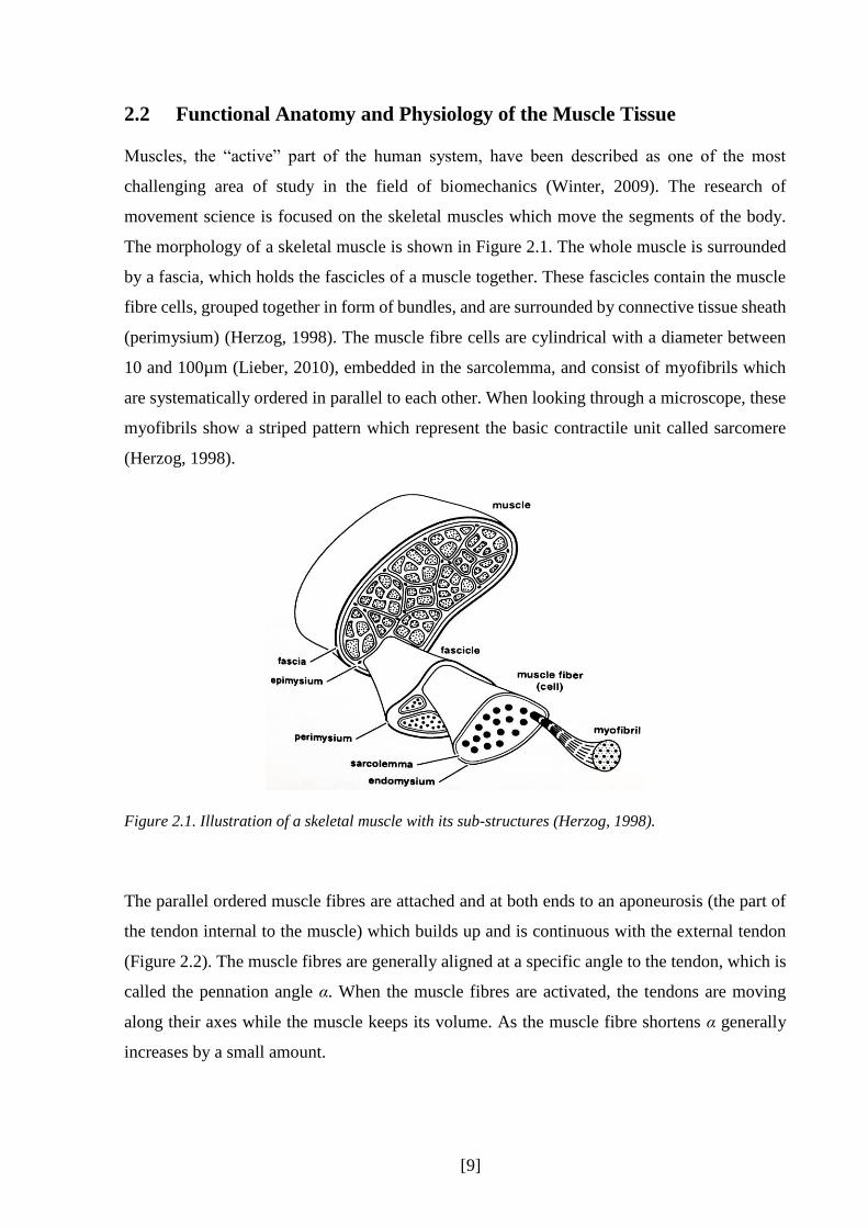
2.2 Functional Anatomy and Physiology of the Muscle Tissue

Muscles, the “active” part of the human system, have been described as one of the most

challenging area of study in the field of biomechanics (Winter, 2009). The research of

movement science is focused on the skeletal muscles which move the segments of the body.

The morphology of a skeletal muscle is shown in Figure 2.1. The whole muscle is surrounded

by a fascia, which holds the fascicles of a muscle together. These fascicles contain the muscle

fibre cells, grouped together in form of bundles, and are surrounded by connective tissue sheath

(perimysium) (Herzog, 1998). The muscle fibre cells are cylindrical with a diameter between

10 and 100µm (Lieber, 2010), embedded in the sarcolemma, and consist of myofibrils which

are systematically ordered in parallel to each other. When looking through a microscope, these

myofibrils show a striped pattern which represent the basic contractile unit called sarcomere

(Herzog, 1998).

Figure 2.1. Illustration of a skeletal muscle with its sub-structures (Herzog, 1998).

The parallel ordered muscle fibres are attached and at both ends to an aponeurosis (the part of

the tendon internal to the muscle) which builds up and is continuous with the external tendon

(Figure 2.2). The muscle fibres are generally aligned at a specific angle to the tendon, which is

called the pennation angle α. When the muscle fibres are activated, the tendons are moving

along their axes while the muscle keeps its volume. As the muscle fibre shortens α generally

increases by a small amount.

[10]

Figure 2.2. Muscle-tendon architecture and the relation of muscle fibres and attached tendons adapted

from Zajac (1989). Angle α represents the pennation angle of the muscle fibres.

A muscle contracts if its fibres get excited by an action potential from a motor neuron causing

an electromechanical stimuli (Herzog, 1998). Motor neurons have their origin in the spinal cord

and terminate on a motor end plate on the muscle fibres (Figure 2.3) (Winter, 2009). Each motor

neuron is connected to a number of muscle fibres which form a motor unit (Herzog, 1998;

Winter, 2009). Dependent on the task of the muscle, these motor units contain a different

number of muscle fibres: for fine control movements the motor neuron would only innervate a

few muscle fibres, while for large powerful muscles and movements with less need of accuracy

the number in muscle fibres is larger (MacIntosh, Gardiner, & MacComas, 2006).

The end of the motor neuron (presynaptic terminal) and the muscle fibre (postsynaptic

membrane) form the neuromuscular junction (Herzog, 1998). When an action potential of a

motor neuron reaches the synapse a chemical reaction is triggered and sodium ions enter the

postsynaptic cell membrane. This causes an overshoot of sodium in the cell and ends in a

depolarisation in form of an action potential traveling along the stimulated muscle fibre at about

5-10m/s (Herzog, 1998). This leads to the release of calcium (Ca2+) ions into the sarcoplasm

around the myofibrils. The increase in Ca2+ in the muscle fibre allows a chemical reaction which

leads to the sarcomere to contract, muscle force to be generated in the muscle and the joint to

move.

[11]

Figure 2.3. Innervation of the muscle through a motor neuron with its origin in the spinal cord, and

ending with motor end plates in the muscle fibres (Lieber, 2010).

The time delay between the initial electrical stimulation of a muscle and the mechanical force

output at the joints is called electromechanical delay (Yavuz, Sendemir-Urkmez, & Turker,

2010). This is dependent on the elastic properties in and around the active muscle tissue and

tendon (myofilaments, tendon, and aponeuroses) as well as the electromechanical processes

(Grosset, Piscione, Lambertz, & Perot, 2009; Yavuz et al., 2010). In the academic literature this

delay is highly discussed (e.g. Blackburn, Bell, Norcross, Hudson, & Engstrom, 2009; Grosset

et al., 2009; Knutson, 2007; Nordez et al., 2009; Rampichini, Ce, Limonta, & Esposito, 2013)

and, depending on the muscle and the participants’ characteristics (e.g. type of muscle fibre,

age, fatigue (Yavuz et al., 2010)), it can lie between 8 and 127ms (Rampichini et al., 2013).

However, it has to be kept in mind that the method with which the electromechanical delay is

measured can result in different values as well (Rampichini et al., 2013; Yavuz et al., 2010).

Information about the morphology and physiology of a muscle and the muscle force generation

are essential for analysing differences between individuals with a musculoskeletal disorder and

a healthy group. It is important to consider the excitation of the muscle to the mechanical output

of the joints as a process with multiple influencing factors which could all lead to a change

between patients and control group. Simplified, this process can be divided in four main stages

(Figure 2.4): the excitation of the muscle tissue through the motor neuron, the chemical

activation in the muscle cell through Ca2+ ions, the actual mechanical force production, and the

visible movement of the segments. Depending on the pathology, restrictions are originated

[12]

primarily through different systems of the body. For example cerebral palsy is primarily a

restriction of the central nervous system (CNS, stage 1), whereas leg deformities are primarily

a change of the skeletal system (stage 4). However, both examples can have secondary effects

on other stages of the force generation which underlines the importance of understanding the

whole process.

Figure 2.4. Schematic illustration of the electromechanical delay and its four main stages, including

measurement methods (top) and the origin of exemplary pathologies (bottom). CNS=central nervous

system, GRF=ground reaction force.

In the academic literature, the terms excitation, activation and force output can be differently

defined, depending on the field of study (e.g. modelling or biology related). For this work these

terms are used to describe following definition (Hicks, Uchida, Seth, Rajagopal, & Delp, 2015):

Excitation: The innervation of the muscle tissue through the motor neuron arriving at the

neuromuscular junction leading to a depolarisation of the T-tubules.

Activation: The release of Ca2+ ions which causes the muscle to contract.

Force output: The muscle produces force, either in isometric or dynamic mode, leading to a

movement or the ability to work against gravity through inertial forces or

antagonistic muscle activity.

[13]

2.3 Development of the Classical Gait Analysis

Human movement is a complex topic and a growing research field. According to Baker (2007)

and Kirtley (2006) Aristotle (384 until 322 BC) was one of the first known scientists to analyse

human walking. It was not until the late 19th and early 20th century, however, that scientific

methods started to be applied to gait analysis simulated by new measurement techniques, such

as the multiple exposure camera (Muybridge, 1907). One of the first experimental studies that

analysed systematically the characteristics of healthy walking was the work of Murray and

colleagues (1964) using interrupted-light photography (Figure 2.5). They provided normative

two-dimensional joint angles of the lower limb during walking for five different age groups

while comparing different age groups as well as groups with different body heights.

Figure 2.5. Photograph showing a participant equipped with reflecting markers which were exposed to

an interrupted light flashing 20 times per second (Murray et al., 1964).

Whilst early interest focused on the analysis of healthy walking, interest in the impact of various

diseases grew throughout in the 20th century, leading to the development of clinical gait analysis

(Andriacchi & Alexander, 2000). Today, gait analysis is widely used in a clinical setting, where

clinicians evaluate the different walking pattern of a specific patient compared to normative

healthy walking (Davis III, Õunpuu, Tyburski, & Gage, 1991). In clinical movement analysis

walking is a commonly used task to compare a patient with normative kinematic and kinetic

data (Perry & Burnfield, 2010). It is a crucial movement impacting the quality of life (Chris

[14]

Kirtley, 2006), the independence and functional status, likely to be restricted by the

consequences of various diseases.

Over 25 years ago a biomechanical model was developed known under the name of the Helen

Hayes (Kadaba et al., 1989) or the Newington Model (Davis III et al., 1991). It has been

integrated into the Vicon motion capture system (PlugInGait) and is known as the Conventional

Gait Model (Baker, 2013). This biomechanical model simplifies the complex anatomical and

mechanical properties of the human body and provides outputs describing the movements that

occur at the different joints during walking. The conventional gait model is divided up into

seven rigid segments, linked together through three degrees of freedom ball and socket joints.

It includes simplified body structures of the pelvis, the femur, the tibia and the foot. Nowadays,

this is the most commonly used model in clinical gait analysis.

A typical gait analysis focuses on the kinematic and kinetic data capture. Kinematic data are

acquired through the recording of the trajectories of reflective markers which are placed on

body landmarks of the body segments to calculate the relation of the segments in a specific

coordinate system, tracked by infrared cameras (Kadaba, Ramakrishnan, & Wootten, 1990).

Kinematics describe the way body segments move in space (segment kinematics) and in relation

to their adjacent segments (joint kinematics). This is possible by implementing a reference

coordinate system into each segment and comparing this to a global coordinate system of the

space (Baker, 2013). If the segments’ orientations in space are known, joint angles, velocities

and accelerations can be calculated (Davis III et al., 1991).

Kinetic data include forces, moments and powers acting on the human body (Baker, 2013).

Newton’s laws describe how the body moves as a consequence of these factors and are

representing the equation of motions (Winter, 2009). One force acting on the body is the ground

reaction force (GRF) which is the response of the ground to the foot contact (Figure 2.6). With

additional information about the kinematics, mass and moments of inertia of the body segments

joint moments can be calculated by a process called inverse dynamics (Bresler & Frankel,

1950).

[15]

2.4 Classical Gait Analysis and Muscle Force

One of the easiest way to get an overview about which muscle group could be active during

walking is to look at the progression of the GRF during the stance phase (Chris Kirtley, 2006).

The position of the GRF in relation to the different joint centres of the lower limb indicates

which muscle group must dominate to oppose the moment arising from the GRF. If the GRF

passes on one side of the joint then the muscles acting across the other side of the joint are likely

to be active. If the GRF passes through a joint then the moments produced by both agonist and

antagonists must be equal and opposite.

Figure 2.6 shows an example for the ankle. At initial contact (A) the GRF passes behind the

ankle joint and is opposed by the dorsiflexors of the ankle. At around foot flat (B) the GRF

passes through the ankle joint centre indicating an equilibrium of muscle forces between the

dorsi and plantarflexors. As stance progresses the GRF moves forward with respect the ankle

joint centre (C) indicating increased force production of the plantarflexors. Whilst giving a

broad overview of muscle activity, however, this method is quite limited. Only the stance phase

of the gait cycle can be analysed, and no effects of acceleration of the body segment is taken

into account.

Figure 2.6. Progression of the ground reaction force vector during normal gait in stance phase (Chris

Kirtley, 2006).

The calculation of joint moments using a full inverse dynamics analysis is required to give a

more accurate indication of the overall net moment produced at a joint. This will arise from

agonist and antagonist muscles and other passive tissues which cross the joint. Inverse

dynamics, however, only indicates the overall joint forces and moments and gives no indication

[16]

of how this arises from the balance of agonists or antagonists or of which muscles within a

specific muscle group are active (Buchanan et al., 2005). In general it is not possible to calculate

individual muscle forces, because more muscles are acting within the body than there are

degrees of freedom (rotations and translations in all three planes) in the joints (Bogey, Perry, &

Gitter, 2005). This is defined as the redundancy problem: the same net joint moment can be

achieved through many combinations of activity in the numerous muscles spanning a joint

(Pandy & Andriacchi, 2010).

The absolute force of a muscle during walking can only directly be measurable with invasive

methods (Figure 2.4) (Bogey, Cerny, & Mohammed, 2003). Such invasive techniques have

been used in the past for human walking in a small number of studies: Komi (1990) recorded

in vivo forces via force transducers inserted in the Achilles tendon, whereas Finni and

colleagues (1998) improved this technique by using an optic fibre inserted into the tendon.

Komi’s technique required, however, a surgical implantation under local anaesthesia whereas

Finni et al. inserted the optic fibre using a sterilised needle using only anaesthetic cream.

Although they improved these techniques it is still generally assumed to be too invasive for

routine clinical use.

[17]

2.5 Electromyography and Muscle Force

Another indirect method has been developed to analyse muscle excitation patterns during

human movements: electromyography (EMG) can record the muscle action potentials which

innervate the muscle (Figure 2.4) (Sutherland, 2001) thereby giving information about the

activation level of a muscle (Shewman & Konrad, 2011). EMG measures muscle excitation

patterns with either surface electrodes, where the electrodes are placed on the skin, or

indwelling electrodes, which are inserted into the muscle (Winter, 2009). EMG is seen as the

“gold standard” in clinical gait analysis to analyse muscle excitations. EMG, however, is not

directly related to muscle forces (Hug, Hodges, & Tucker, 2015) as it measures the electrical

rather than the mechanical activity (Whittle, 2001). The relationship between excitation and

force production is complex and still unclear, leading to differing conclusions (De Luca, 1997;

Pandy & Andriacchi, 2010). Some studies show a linear correlation between the amount of

EMG excitation and produced muscle force in isometric (A. L. Hof & van den Berg, 1977;

Johnson, 1978; Lippold, 1952), or isotonic conditions (Bigland & Lippold, 1954), whereas

other studies disagree (Komi & Viitasalo, 1967) or give inconsistent findings between different

muscles (Alkner, Tesch, & Berg, 2000; Woods & Bigland Ritchie, 1983). EMG measurements

are also sensitive to a number of experimental factors such as skin preparation or the nature of

the tissues between electrode and muscle.

Surface EMG is only applicable for larger superficial muscles. For deeper or smaller muscles

it is necessary for a fine wire to be directly inserted into the muscle tissue. One of the

disadvantages here lies in a small recording area in the muscle, which may not represent the

whole muscle (Soderberg & Cook, 1984). It also requires specific training of a practitioner who

is clinically qualified for routine clinical use.

[18]

2.6 Modelling and Simulation

A more recent way to analyse muscle physiology and, therefore, as well the force a muscle

produces is the estimation of muscle forces via mathematical models. A musculoskeletal model

is additionally used to present the anatomical structures while calculations and optimisation

criteria simulate a specific movement. Model, simulation, and estimation are defined in detail

as follows (Hicks et al., 2015):

Model: A model defines a set of mathematical equations that describe a static,

physical system. This may be the human anatomy presented through a

neural and muscular system acting on a rigid multibody skeletal

structure.

Simulation: A simulation uses a model to be able to study a specific motion by

imitating a behaviour or process. Therefore, it describes how something

dynamically functions, for example how a human anatomical system is

able to walk or jump.

Estimation: An estimation defines a close guess of the actual values through

calculations and defines the most plausible value of a parameter.

2.6.1 Musculoskeletal Models

A musculoskeletal model is a set of mathematical equations that describe a physical system

(Hicks et al., 2015), which may represent the human neuro and/or muscular system. This

includes the action of this active system on the rigid multibody skeleton with interaction of the

ground. It may represent, therefore, the muscular-tendon structure, the origin and insertion of

this complex, and other force-dependent characteristics.

In the 60ies and 70ies, when computer programming was developing, researchers began to

model human locomotion at a theoretical level by developing optimisation programmes and

control theories (Chow & Jacobson, 1971). Seireg and Arivkar (1973) and Crowninshield and

Brand (1981) are one of the first to implement cost functions to optimise estimated muscle

forces of the lower limb. It is only relatively recent, however, that breakthroughs in the research

of robotic control technique and biomechanical simulation have made musculoskeletal

modelling a practical proposition for clinical gait analysis (Delp et al., 2007). Such techniques

solve the redundancy problem using mathematical models to estimate muscle activations and

[19]

forces (Buchanan et al., 2005) using experimental movement analysis data as well as subject

specific anthropometric data. The skeleton and the muscles are represented in form of a

musculoskeletal model (Erdemir et al., 2007), which defines the number and masses of

segments of the model, the degrees of freedom of the joints, and the number of muscles and

their properties.

The bony structure is modelled as a number of rigid bodies articulated through joints in a 2D

or 3D space. These bony segments are defined by their mass, moments of inertia, centre of mass

location, and the joints by the number and nature of the degrees of freedom and permitted range

of movement. These anthropometric values are taken from older cadaver studies or from the

digitalisation of bony structures (Delp et al., 1990). Muscles are modelled as being attached to

the segments at an origin and an insertion on specific landmarks. Straight line paths are assumed

for most muscles but via points (Figure 2.7) can be included where muscles wrap around bones

or other muscles or are constrained by a retinaculum (Au & Dunne, 2012; Delp, 1990).

Figure 2.7. Different representation of muscles: some of the muscle patters are only defined through

origin and insertion, e.g. the soleus (left muscle), others are represented through more than one line

segment including via points, e.g. the peroneus longus (right muscle) (Delp et al., 1990).

Further characteristics of the muscle-tendon units are needed to create muscle-driven

simulations (Delp et al., 2007) such as the optimal length of a muscle fibre (at which it produces

the maximum force), the pennation angle of the muscle, the maximum force a muscle can

produce, the length of a tendon where it starts to generate force (tendon slack length) and the

elasticity of the tendon. The muscle activation-contraction dynamics specify how force

generation within the fibres is dependent on fibre length and lengthening velocity. Arnold and

colleagues (2013) define the overall muscle forces as follows,

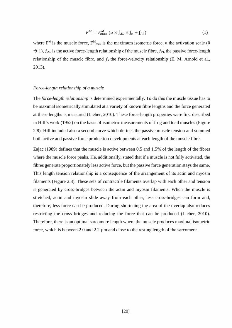
[20]

𝐹𝑀 = 𝐹𝑚𝑎𝑥𝑀 (𝑎 × ƒ𝐴𝐿 × ƒ𝑣 + ƒ𝑃𝐿) (1)

where FM is the muscle force, FMmax is the maximum isometric force, α the activation scale (0

1), ƒAL is the active force-length relationship of the muscle fibre, ƒPL the passive force-length

relationship of the muscle fibre, and ƒv the force-velocity relationship (E. M. Arnold et al.,

2013).

Force-length relationship of a muscle

The force-length relationship is determined experimentally. To do this the muscle tissue has to

be maximal isometrically stimulated at a variety of known fibre lengths and the force generated

at these lengths is measured (Lieber, 2010). These force-length properties were first described

in Hill’s work (1952) on the basis of isometric measurements of frog and toad muscles (Figure

2.8). Hill included also a second curve which defines the passive muscle tension and summed

both active and passive force production developments at each length of the muscle fibre.

Zajac (1989) defines that the muscle is active between 0.5 and 1.5% of the length of the fibres

where the muscle force peaks. He, additionally, stated that if a muscle is not fully activated, the

fibres generate proportionately less active force, but the passive force generation stays the same.

This length tension relationship is a consequence of the arrangement of its actin and myosin

filaments (Figure 2.8). These sets of contractile filaments overlap with each other and tension

is generated by cross-bridges between the actin and myosin filaments. When the muscle is

stretched, actin and myosin slide away from each other, less cross-bridges can form and,

therefore, less force can be produced. During shortening the area of the overlap also reduces

restricting the cross bridges and reducing the force that can be produced (Lieber, 2010).

Therefore, there is an optimal sarcomere length where the muscle produces maximal isometric

force, which is between 2.0 and 2.2 µm and close to the resting length of the sarcomere.

[21]

Figure 2.8. Left: force-length curve adapted from Hill (1952), right: force-sarcomeres length

relationship from Lieber (2010).

It has to be kept in mind, however, that this curve is generated through isometric contractions.

To understand how a muscle performs in dynamic movements the force-velocity relationship

has to be taken into consideration as well (Lieber, 2010).

Force-velocity relation of the muscle

In Zajac’s work (1989) the force-velocity relation of the muscle fibres is discussed and

illustrated in a graph (Figure 2.9). The muscle reacts differently to velocity if the fibres getting

shorten or lengthened. If the muscle shortens then the force reduces with shortening velocity

until it reaches its maximum shortening velocity (vm) after which the muscle cannot generate

any fore at all. On the other side, if the muscle fibres are lengthening (which will occur if the

externally applied force is greater than that which can be exerted by the muscle) then the

maximum force increases quite rapidly to a value of about 1.8 of peak active isometric force

(FM0) at optimal fibre length.

[22]

Figure 2.9: The force-velocity relation of muscle fibres adapted from Zajac (Zajac, 1989).

2.6.2 Mathematical Models: Inverse and Forward Dynamics

A mathematical model describes mathematical equations which enable the estimation of motion

of a musculoskeletal model. This is operated by a simulation with which the motion and forces

of a system can be analysed (Hicks et al., 2015). Biomechanical modelling to estimate muscle

force generation during human movement can be done by inverse and forward dynamics

(Erdemir et al., 2007). Inverse dynamics (e.g. static optimisation) calculates the forces and

moments that must have acted at the joints in order to generate the measured ground reaction

and body segment accelerations (Figure 2.10). This is a two-step process, as, firstly, the joint

torques (e.g., moments) will be calculated with the help of Newtonian laws (equation of

motions), and secondly, the muscle forces are estimated while taking the muscular-tendon

properties into account. Forward dynamics, in turn, estimates the body segment accelerations

that will be generated by derived muscle forces according to the equation of motions. The

muscle forces have been estimated before by a given set of muscle states and the muscular-

tendon properties. This whole process allows an estimation of how the body will move

dependent over a particular time frame (Erdemir et al., 2007; Lin et al., 2012).

Inverse dynamics to estimate muscle forces is computationally much simpler and quicker and

is known to be more robust to measurement errors (Lin et al., 2012). It, however, can only give

insights into the measured movement independently at each instance in time. Forward

dynamics, whilst more challenging, is able to give insights into how the body would move if

different muscles had been active. Both techniques are affected by the redundancy problem

(muscles spanning the joint > degrees of freedoms, chapter 3.3.6). Cost functions which

minimise a specific performance criterion solving this problem by optimising the amount of

each individual muscle activation (Glitsch & Baumann, 1997). For the purpose of walking a

[23]

variety of criteria such as the minimisation of the overall muscle activation, force, or power, or

of energy expenditure or oxygen consumption are used (Chow & Jacobson, 1971).

One of the forward dynamic approaches is EMG-driven modelling. In this, measured EMG

excitations are input into the simulation alongside one of the optimisation criteria listed in the

preceding paragraph (Lloyd & Besier, 2003). This method is limited, however, both by the

experimental difficulties in obtaining quantitative EMG data and by the limited understanding

of the detailed relationship between the EMG signal and muscle force generation. A more

detailed description of mathematical models can be found in chapter IV.

Figure 2.10. Schematic flow chart of inverse (A) and forward dynamics (B), adapted from Erdemir et

al. (2007).

2.6.3 Development and Limitations of Models and Simulations

Two primary research groups have been working in the last few years on the development of a

musculoskeletal model and simulations to estimate muscle activations and forces in human

movement science. These are the Stanford University group with Scott Delp and the group at

the University of Texas with Frank Anderson and Marcus Pandy. All three main developers are

mechanical engineers, however, work in the field of movement science.

The Anderson and Pandy model started to develop in the late 80ies (Pandy & Berme, 1988a,

1988b) with the work of Pandy to create a model which simulated the movement of the human

walking in stance and swing phase. In 1990, Pandy and colleagues published a paper (Pandy,

Zajac, Sim, & Levine, 1990) about 2D optimal control for maximum height jumping. The

[24]

musculoskeletal model was designed as a four segment body representing one leg and the hip,

which was articulated by eight Hill-type muscle-tendon units. The muscular-tendon dynamics

were adapted from Zajac (1989), whereas the muscular properties (geometry, maximum

isometric force…) were imported from Brand and Wickiewicz works (Brand et al., 1982;

Brand, Pedersen, & Friedrich, 1986; Wickiewicz, Roy, Powell, & Edgerton, 1983). This was

the ground work for the latter model of Anderson and Pandy used to estimate muscle activations

and forces for a 3D maximum vertical jump (Anderson & Pandy, 1999) and during human

healthy walking (Anderson & Pandy, 2001a, 2001b) while comparing different mathematical

models (static optimisation, forward dynamics).

This final model of Anderson and Pandy used information about muscle parameters, especially

the origin and insertion of the muscle-tendon complex, of the Delp model from 1990. Delp

published through his PhD thesis a computer graphic-based musculoskeletal model which was

able to be used in orthopaedic surgery simulations. This model referred as well to the muscle

geometrics of Brand and Wickiewicz, however, Delp realised that especially for extreme

flexions of the ankle, knee, and hip the muscles did not run around the bones but passed through

the joint. This was solved by introducing points and wrapping points into the model, so that the

definition of some of the muscles was not only defined by the two origin and insertion point

but also by points along the muscle (Delp, 1990; Delp et al., 1990). More information about the

Delp model and its enhancements can be found in chapter IV.

At the time that these models originated, the engineers were quite enthusiastic about their

development of musculoskeletal models to estimate muscle forces in various movement and

conditions. What, however, stayed yet in the background was the verification and especially

validation of these models. Model and simulation verification and validation is crucial for

implementing such musculoskeletal models into the clinical movement analysis. Today’s

research is aware of the important verification and validation (e.g., E. M. Arnold et al., 2013).

To be able to implement these techniques into a clinical gait analysis routine the existing

musculoskeletal models and simulations of the estimation of muscle forces need to be validated

according to the strength and weaknesses of these models. This gets more important as

musculoskeletal modelling in the field of movement science (Hicks et al., 2015) as well as in

clinical gait analysis (e.g., Arch, Stanhope, & Higginson, 2015; Lerner, Board, & Browning,

2015; Skalshoi et al., 2015) is increasing. Still, the literature is lacking in a straight forward and

standardised validation procedure. The first attempt to systematise a controlled verification and

[25]

validation process for musculoskeletal modellers is the work of Hicks and colleagues (2015)

which will be briefly presented in chapter 2.6.3.1.

Another limitation of such models and simulations is present in the literature. A lot of different

factors may influence the estimation’s outcome, like the experimental data, the musculoskeletal

model or the cost functions used in the optimisation process. This may result in different muscle

force profiles while using different experimental or modelling and simulation protocols. For

example, both studies of Glitsch and colleagues (1997) and Bogey and colleagues (2005)

estimated the muscle force of the tibialis anterior during walking but resulted in different force

profiles throughout the gait cycle. Several factors differ between these studies like the

mathematical model used for the prediction as well as other factors related to the

musculoskeletal model. Less is known about the extent of influence of individual factors which

makes it hard to find the protocol most suitable for the clinical gait analysis. Also, the

comparison between laboratories is impossible without a standardised protocol as too many

factors may play an influencing role. To date, such protocol has not yet been developed for the

clinical gait analysis.

2.6.3.1 Validation Process for Musculoskeletal Modelling and Simulations

Validation answers the question if the correct equations are being solved (Hicks et al., 2015)

and, therefore, to which degree the real world is represented by the model (Thacker, 2001).

Although musculoskeletal modelling and simulation have been developed over the last 25 years

in the field of movement science, the approach still lacks in a good verification and validation

which allows a wider implementation in the clinic and a wider impact on healthcare (Hicks et

al., 2015). Important for a good validation process is the formulation of a research question

which the model and simulation is able to answer. Therefore, the methods needs to be tested

and a validation plan needs to be designed (Hicks et al., 2015). But also a verification of the

equations is from great importance that it is sure the equations are solved correctly. In case an

algorithm has been implemented wrongly this may lead to incorrect simulations.

Open source software codes can be reviewed and verified directly which makes this kind of

software attractive. If a new protocol has been created to estimate muscle forces to analyse a

specific pathological condition on gait pattern it is important to compare results to existing

muscle force estimations in the literature. In the case this is a novel approach, it is recommended

to test the protocol on healthy adults as well to be sure that similar results are received than

[26]

many other walking simulations in the literature (Hicks et al., 2015). On the contrary, if an

existing protocol is chosen for a study it needs to be clarified that this protocol is suitable for

the research question.

A validation process for modelling and simulations of human movement may be performed by

the comparison with independent experiments or other models (Hicks et al., 2015), however,

this approach is problematic (Delp, 1990). Direct validation is only possible with invasive

methods and these cannot be applied in a clinical setting (Pandy & Andriacchi, 2010). With

good quality experimental data joint moments as well as the kinematics and therefore the

moment arms of the muscles can give first indications about which muscle must be active. This,

however, does not give clear details about the exact muscles especially because of the

redundancy problem and potential agonists and antagonists being active.

Although EMG excitations are not directly comparable with muscle force estimations in the

magnitude of force, EMG muscle excitations provide a validation tool for the temporal

characteristics of muscles estimated by mathematical models. This has been used several times

in the literature (Erdemir et al., 2007), for example from Glitsch and Baumann (1997), who

used a static optimisation model, where surface EMG of the lower limb was captured on the

participants parallel to the experimental data capturing. Neptune and colleagues (2008) in a

dynamic optimisation study even used surface activation of the muscles soleus and

gastrocnemius to validate qualitatively changes in muscle force estimations throughout

different walking velocities. However, when using this validation technique the limitations of

EMG need to stay in mind while interpreting results.

[27]

2.7 Statement of the Problem

Summarising the above information, integrating musculoskeletal modelling into clinical gait

analysis could greatly enhance its potential by improving the patient’s quality of life in long

term and reducing the costs for the health care system (Delp et al., 2007; Lin et al., 2012).

Classical gait analysis and electromyography have two limitations which have not yet been

resolved: firstly, the redundancy problem which describes the problem that more muscles

spanning a joint than degrees of freedom exist as well as the existence of bi-articular muscles

which cannot be solved via simple net joint moments calculations, and, secondly, the limitations

of EMG measurements monitoring only the sequence and timing of muscles activities as well

as to some extent a “more on” and “more off” activation but not the exact amount of individual

force production (Pandy & Andriacchi, 2010).

The integration of musculoskeletal modelling could augment the classical approach in clinical

gait analysis and help to enhance clinical decision making in an interdisciplinary team. By

solving the redundancy problem, these models can estimate each single muscle force which

completes a simple surface EMG measurement. Also, with such models, post-operative

prognoses might be given which help the clinicians to decide for the right treatment.

Furthermore, including mathematical models into a standardised clinical gait analysis routine

can improve creating and adapting rehabilitation protocols by gaining more and better

knowledge about the behaviour of the muscular system during walking. However, modelling

approaches to estimate muscle activation and forces have not yet made their way into the

clinical movement analysis, mainly because of two reasons: firstly, there exists a high variety

of models and methods which makes the decision for a clinician hard to define the best solution;

and second, a standardised protocol which can be easily implemented into a routine processing

has not yet been established, also because modellers and clinicians have different approaches

and foci on their studies.

Also, although musculoskeletal modelling exists for a while in the scientific literature, the

validation of these methods lacks in its accuracy and quality. This, however, is crucial to be

able to implement a model into a clinical setting and to widen the impact on healthcare.

Therefore, it is of great interest to resolve these limitations which would make it possible for

clinicians to understand and apply a protocol which includes mathematical modelling and the

estimation of muscle activations and forces.

[28]

2.8 Research Question

This PhD thesis aims to develop and test a protocol to estimate muscle forces during human

walking for the lower limb muscles which can be applied in the classical clinical gait analysis.

The following steps need to be undertaken to understand the literature and to locate an

appropriate musculoskeletal model with a mathematical model suitable for the clinical gait

analysis:

1. Different mathematical modelling approaches to estimate muscle forces exist in the

literature but less is known about the relation to each other and to clinical gait analysis.

Therefore, a systematic review is undertaken covering academic studies estimating

muscle forces in human healthy walking. It identifies the current state-of-the-art in

modelling and simulation and examines how the variability between different

approaches affects the consistency in estimated muscle forces. Furthermore, this review

identifies the modelling approaches most likely suitable for the use in clinical gait

analysis.

2. After identifying appropriate models for a potential standardised protocol with which

muscle force estimations can be integrated into the clinical routine processing,

musculoskeletal models need to be adapted to the clinical needs. Therefore, an adequate

software needs to be selected with which these demands are possible.

3. The final step tests this musculoskeletal model as well as chosen mathematical

approaches in the laboratory on a healthy population group. Static and dynamic trials

are captured to collect experimental data required for the input in these models. Potential

influencing factors on the estimation’s outcome (e.g. experimental data,

musculoskeletal model…) need to be identified and controlled that the final outcome

can be drawn down to the method chosen for muscle force estimation. The results will

be validated with experimental data (joint torques, EMG) to analyse the potential of

these models.

Finally, these steps can help to clarify the potential of existing musculoskeletal modelling

approaches related to clinical gait analysis and identify if and which further steps are needed to

be undertaken to introduce these models into the clinical daily routine. Moreover, substantial

body of this work can help to close the gap between modellers and clinicians and make a clear

transition from the modelling approaches to the clinical needs. These results will further

contribute to the current knowledge about muscle force analysis in clinical gait analysis.

[29]

Therefore, the research questions which this work will discuss are:

1. What is the state-of-the-art in movement science to estimate muscle forces and joint

moments which act on the lower limb joints during walking?

2. Are there experimental parameters and/or parameters related to modelling and

simulation which may affect the estimation’s outcome? Which parameters need to be

taken into consideration to create a standardised protocol which implements the

estimation of muscle forces in the clinical gait analysis?

3. Which mathematical model, musculoskeletal model, and simulation environment to

estimate muscle forces are the one most suitable for the clinical routine according to the

literature?

4. Is it possible with the current facilities to estimate individual muscle forces on a human

healthy population on the lower limb and are the results comparable to parallel captured

surface EMG?

[30]

CHAPTER III

3 Systematic Review of Muscle Force Estimation in Gait

Analysis

As described in the previous chapters, knowing the force profiles of individual muscles during

walking has the potential to help to identify various musculoskeletal impairments (orthopaedic

restrictions, dysfunction of the nervous system etc.) and can give a better understanding about

the underlying mechanisms and the impact of these impairments on the musculoskeletal system.

Currently available clinical measurement systems incorporate inverse dynamic techniques

which can give insights into the net muscle forces acting across a joint but are unable to

distribute these across the range of muscles. EMG measurements capture the arriving electrical

impulse innervating the muscle which can give information about the muscle activation profile

as well as the degree of muscle activation by normalising the signal to a maximum isometric

contraction. They are, however, limited in practice to a small number of muscles and

considerable assumptions are required to estimate the associated force production in the muscle.

These experimental techniques are, therefore, severely limited in the information they can give

us about force generation in individual muscles. In-vivo methods (e.g. force transducers, Komi,

1990) are needed to capture the muscle forces directly, but are highly invasive and not

applicable in a clinical setting. Muscle force estimation with mathematical models could,

therefore, fill this gap and give more detailed information about the muscle activity and the

corresponding force production of a wide range of muscles.

Until now, no standardised protocol exists to estimate muscle forces as a part of routine clinical

gait analysis. Before muscle force estimation can be implemented into the clinical gait analysis,

it is crucial to understand the state-of-the-art of mathematical models which estimate the force

characteristics of lower limb muscles during walking. Numerous musculoskeletal and

mathematical models are available providing different approaches to the estimation of muscle

forces (Anderson & Pandy, 1999, 2001b; Lin et al., 2012). Additionally, different experimental

data (marker trajectories, ground reaction forces, or electromyography) are frequently used as

an input into these models to be able to estimate muscle forces. Furthermore, different cost

[31]

functions can be applied into the simulation to optimise the estimation by minimising a range

of factors (e.g. the sum of all muscle forces squared).

To be able to give an overview about these mathematical models and their underlying

musculoskeletal models and principles a detailed review of the academic literature is needed.

Available modelling techniques need to be analysed to identify potential mathematical

approaches and musculoskeletal models which may suit the clinical gait analysis routine. Inter-

and intra-model variability needs, therefore, to be investigated and factors which may influence

the estimation’s outcome need to be identified.

This systematic review seeks, therefore, to identify and analyse studies which have estimated

muscle forces in the lower limbs during walking. Whilst the ultimate aim of clinical gait

analysis is to provide such data for patients with a range of conditions, the starting point of such

an analysis is an ability to generate robust data for healthy adults, which the review will focus

on. The review will, thus, describe the state of the art in muscle force estimation in order to

determine where consensus amongst studies exists using similar or different modelling

approaches and to identify areas where these studies give different results. The overarching aim

will be to identify one or more modelling approaches which could feasibly be applied in clinical

gait analysis and to propose recommendations for a standardised protocol for the estimation of

muscle forces during walking.

[32]

3.1 Introduction into Systematic Reviews in Movement Science

Cochrane, an independent network of scientists working in the field of health science, has

defined a systematic review as follows:

“A systematic review attempts to collate all empirical evidence that fits pre-

specified eligibility criteria in order to answer a specific research question. It uses

explicit, systematic methods that are selected with a view to minimizing bias, thus

providing more reliable findings from which conclusions can be drawn and

decisions made.” (Higgins & Green, 2011)

In addition, five key characteristics of a systematic review have been stated as (Higgins &

Green, 2011):

1. a clearly stated set of objectives with pre-defined eligibility criteria for studies;

2. an explicit, reproducible methodology;

3. a systematic search that attempts to identify all studies that would meet the eligibility

criteria;

4. an assessment of the validity of the findings of the included studies, for example through

the assessment of risk of bias; and

5. a systematic presentation, and synthesis, of the characteristics and findings of the

included studies.

Thus, a systematic review gives an appropriate, detailed and unbiased overview about a specific

topic. By rating studies and using a quality assessment tool each included paper is evaluated

according to the criteria of interest. In the case of human movement analysis a systematic review

can give an overview of specific biomechanical procedures and analyse the consistency of

results produced by these across the literature.

Several systematic reviews in human movement science involving walking have already been

published. McGinley and colleagues undertook a systematic review about inter-session and

inter-assessor reliability for gait analyses (2009). They set the focus exclusively on kinematic

measures of the lower limb. One year later, another systematic review about gait analysis has

been published which investigated the soft tissue artefacts of the lower limb (Peters, Galna,

Sangeux, Morris, & Baker, 2010). Latter study has been cited close to 100 times, whereas the

[33]

study of MyGinley et al. has been cited over 250 times (google scholar, web of science

09.01.2016), which shows the importance of such studies in the field of movement science.

Good quality systematic reviews are here crucial to present the state-of-the-art as well as point

out strength and weaknesses to develop the field further to ensure a high quality performance

and to achieve protocols which can be applied in clinical settings.

One reason that muscle force estimations are not yet implemented into a clinical gait analysis

routine is the lack of standardised protocols and processing tools. Another reason are the known

limitations (e.g. sensitivity to musculoskeletal geometry, muscle and tendon characteristics and

the modelling of the foot-floor interaction, see chapter II). If the effects of these limitations of

musculoskeletal modelling are known, they can be taken into consideration while interpreting

the results which might make these methods useful in the clinic even if the results cannot be

regarded as completely robust. Such a review will also help the developers to improve the

protocols according to the needs of a clinical routine so that mathematical models to estimate

muscle forces may be able to be implemented in the clinic.

Factors affecting muscle force estimation are those related to the experimental and estimation’s

method used, to the parameters used to describe the person, and to test conditions such as the

walking velocity (C Kirtley, Whittle, & Jefferson, 1985; Schwartz, Rozumalski, & Trost, 2008),

or the placement of the markers (Kadaba et al., 1989; Szczerbik & Kalinowska, 2011).

Additionally, there exists natural inter-subject and intra-subject variabilities in movement

patterns (McGinley, Wolfe, Morris, Pandy, & Baker, 2014; Schwartz, Trost, & Wervey, 2004)

which needs to be taken into account when analysing the consistency between individuals and

across studies. To gain an overview across the academic literature about muscle force

estimations during walking and the consistency amongst mathematical models, it is important

to consider these factors in the review.

Therefore, a systematic literature database search will be undertaken to identify studies which

estimate muscle forces of the lower limb during healthy adult walking. Many modelling

approaches calculate net joint moments first and then apply some technique to distribute these

across the various muscles crossing the joint. To give insight into whether differences in results

are a consequence of the moment calculation or the force distribution stages the survey will

include studies which included the calculation of joint moments on the lower limb during

healthy adult walking. A customised scoring principle will be applied to qualitatively rate and

[34]

analyse the identified joint moment and muscle force studies according to their methodology

and reporting of the musculoskeletal model and simulation.

Graphs presenting the joint moments and muscle forces of the lower limb will be extracted,

digitised and analysed according to the variability of their profiles. Possible influencing factors

on the estimation’s output will be detected which will help to define parameters which are

important for the creation of a standardised protocol in the clinic. The consistency between joint

moment profiles compared to the profiles of estimated muscle forces will help to understand

the differences between the well tested inverse dynamics method to calculate joint moments

and the new approach of different mathematical models to estimate muscle forces. Inter- and

intra-mathematical model force estimation variability will be compared and analysed which

enables to identify the mathematical model most usable for the estimation of muscle forces in

the clinical gait analysis routine and helps to give recommendations for a standardised protocol

for the clinical use.

Summarised the three main aims of this systematic review are:

1. The identification and qualitative rating of studies estimating joint moments and muscle

forces during human healthy adult walking.

2. The comparison of variability between joint moment and muscle force profiles of the

lower limb during walking from different studies.

3. The definition of one or more mathematical model(s) most suitable for the application

into clinical practise and the recommendations for a standardised protocol which

includes the estimation of muscle forces.

[35]

3.2 Methods

A systematic review is bounded to specific methodical characteristics. This includes a

systematic study search using topic specific databases and a systematic inclusion-exclusion

procedure undertaken by more than one reviewer. In the sections of this chapter, these steps are

defined and split up as follows: search strategy, selection criteria, quality assessment, and data

synthesis. Selection criteria were composed along with the PICO questions (Participants,

Intervention, Comparison, Outcome), which represent four main criteria defined in the

Cochrane Handbook for Systematic Reviews of Interventions (Higgins & Green, 2011).

3.2.1 Literature Search

3.2.1.1 Search Strategy

To locate relevant papers, the following scientific databases were used, all associated with

either mathematic modelling, biomechanics, movement science or health:

- Ovid including Medline (1990-Jan. 2013) and AMED (1990-Jan. 2013).

- EBSCO, including CINHAL (1990-Jan. 2013) and SPORTDiscus (1990-Jan. 2013).

- Web of Knowledge (1990-Jan. 2013).

The oldest publication year was set to 1990 corresponding to the first reports of practical

mathematical modelling and simulation procedures using experimental input data (Delp et al.,

1990) and the first standardised musculoskeletal models which could be applied during walking

(Delp, 1990; Pandy & Berme, 1988a). A free keyword search was undertaken with additional

Medical Subject Headings (MeSH). These are additional search strategies, in which the

researcher has used specific medical vocabulary-based search terms (Higgins & Green, 2011).

Figure 3.1 gives an overview of the keywords which were included in the database search. They

are organised in the three main categories: gait variables, measurement methods and output

variables. These keywords cover the description of the estimation of lower limb joint moments

and muscle forces of healthy human walking. Within each main category the keywords were

handled as an “OR” boolean operation: at least one keyword out of this keyword group needed

to appear in the title or abstract of a paper to be included. These three categories were then

linked with an “AND” Boolean operation. This means that at least one keyword out of each

main category had to appear. Proximity operations like “NEAR” or “NEXT” could additionally

isolate terms consisting of more than one keyword. As an example the term “musculoskeletal

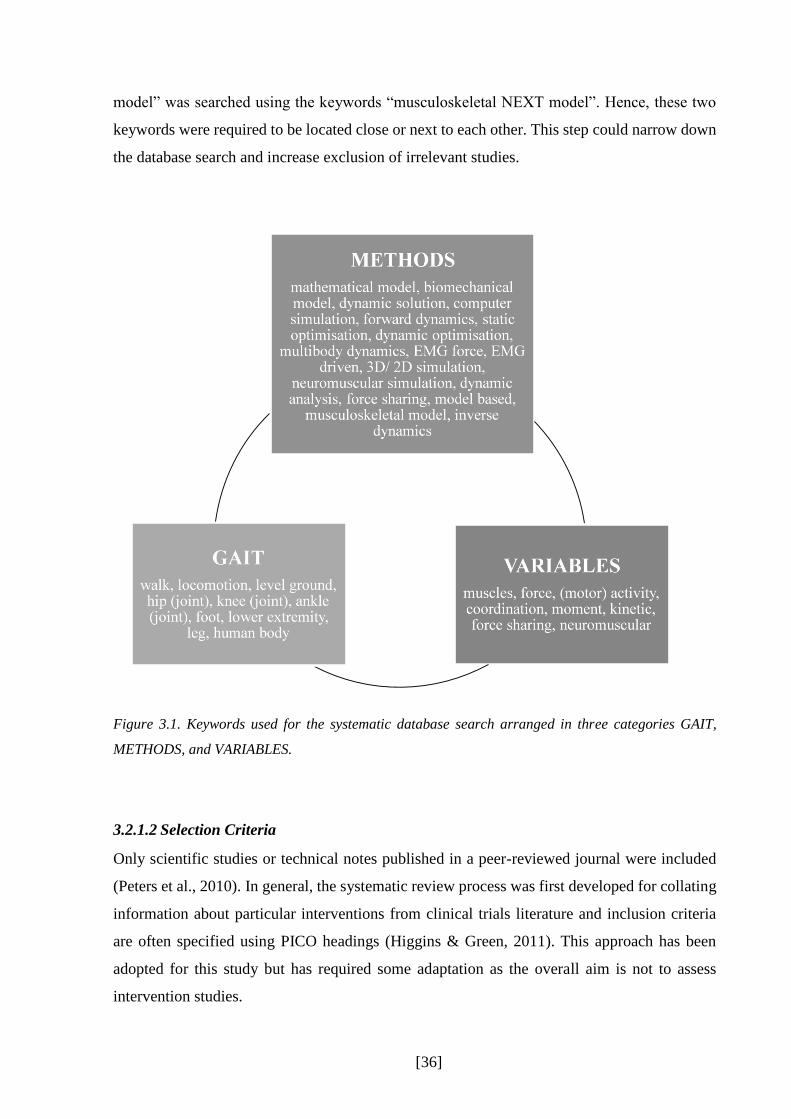
[36]

model” was searched using the keywords “musculoskeletal NEXT model”. Hence, these two

keywords were required to be located close or next to each other. This step could narrow down

the database search and increase exclusion of irrelevant studies.

Figure 3.1. Keywords used for the systematic database search arranged in three categories GAIT,

METHODS, and VARIABLES.

3.2.1.2 Selection Criteria

Only scientific studies or technical notes published in a peer-reviewed journal were included

(Peters et al., 2010). In general, the systematic review process was first developed for collating

information about particular interventions from clinical trials literature and inclusion criteria

are often specified using PICO headings (Higgins & Green, 2011). This approach has been

adopted for this study but has required some adaptation as the overall aim is not to assess

intervention studies.

[37]

Participants

Studies were included if they involved healthy adult participants. Studies which included

healthy participants as a control group for comparison with another patient group were included

and data from healthy participants extracted. The maximum age was set to 60 years as walking

kinematics (Winter, Patla, Frank, & Walt, 1990) and muscle force capacity (Hughes et al., 2001;

Izquierdo, Aguado, Gonzalez, López, & Häkkinen, 1999) are known to change beyond this age.

Intervention

This study is focussing on joint moment and muscle force estimation techniques rather than a

specific intervention so these criteria specify the techniques used.

Studies reporting estimates of joint moments and/or muscle forces for individual healthy

humans calculated from data captured during overground walking were included. Studies

presenting predictive simulations which were not based on data from individuals were

excluded. No gait analyses on a treadmill were accepted as it may have changed the

participants’ walking pattern (S. J. Lee & Hidler, 2008). Studies were only included if

experimental data, joint kinematics and kinetics data and/or EMG activations had been captured

within the researchers’ laboratory (no experimental data from external laboratories or

previously published databases). This diminished the influence of unknown variables and

allows to extract studies with a known measurement protocol.

Comparisons

This category is specific to clinical interventions and not really relevant to this review of

modelling and simulation techniques. Some studies, however, do compare different

combinations of models and simulations applied to the same patient data. In this results from

all modelling and simulation approaches were included.

Outcome

In order to facilitate the objective of comparing time varying muscle force estimations based

on different modelling approaches, only studies providing graphical or numerical data of time

varying muscle force estimations over the entire gait cycle or a defined part of the gait cycle

were included.

[38]

3.2.1.3 Search Process

After extracting potential studies which were located in the chosen databases, titles and

abstracts of these papers were scanned on relevancy by two reviewers (Ursula Trinler, Richard

Baker) and if not suitable excluded from the review. In case one of the categories could not be

fulfilled, the paper was excluded. If a PICO question could not be positively or negatively

answered due to missing information in the title and abstract, the study was included into the

next step for clarification. After scanning title and abstracts alongside with these criteria it was

then decided if these studies were included or excluded for the next step of the systematic

review: the quality assessment tool. Inclusion criteria are summarised in Table 3.1. Studies

which fulfilled these six essential criteria were finally included into the systematic review.

Table 3.1. Summarised inclusion criteria which decide for studies suitable for the systematic review.

Inclusion Criteria

1 Participants had to be healthy adults.

2 The movement analysed had to be walking.

3 No treadmill was allowed to be used for experimental data collection.

4 Lower limb joint moments or muscle forces had to be included.

5 Joint moment or muscle force patterns had to be expressed in a graph normalised to

a defined part of the gait cycle.

6 The inclusion or the tracking of experimental data had to be part of the modelling

process. Experimental data for input into the simulation needs to be own captured

data.

3.2.2 Quality Assessment Tool

Studies which passed the screening of title and abstract were fully evaluated by the same

reviewers according to the criteria described above. All these included papers were subjected

to a customised quality assessment carried out independently by the two reviewers. This step

helped to define the state of the art of musculoskeletal modelling compared to joint moment

calculations and its potential to include these existing protocols into a clinical gait routine. A

[39]

structured quality assessment tool was designed by combining items from similar tools created

for kinematic quality studies (Peters et al., 2010) and randomised and non-randomised clinical

interventions (Downs & Black, 1998; Ridgewell, Dobson, Bach, & Baker, 2010). Items specific

to muscle modelling and simulation were created specifically for this study.

The quality assessment tool is structured to cover nine main items which were applied for all

extracted studies and a further three for studies which incorporated EMG measurements. Some

of the items are further divided in relevant sub-items (Figure 3.2). These items cover the

structural quality of the paper, the description of the protocol and technical details as well as

the presentation of the results. Sub-items’ maximum scoring is defined in Figure 3.2. The score

of an item and its sub-items were summed up and transformed in a percentage of the maximum

possible score. The overall score was then the average of these relation scores which allows the

highest score to be 100%, the lowest to be 0%.

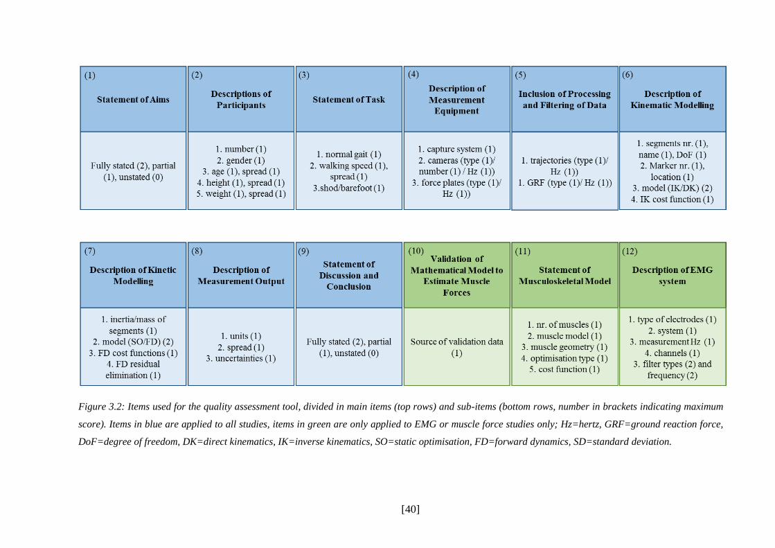
[40]

Figure 3.2: Items used for the quality assessment tool, divided in main items (top rows) and sub-items (bottom rows, number in brackets indicating maximum

score). Items in blue are applied to all studies, items in green are only applied to EMG or muscle force studies only; Hz=hertz, GRF=ground reaction force,

DoF=degree of freedom, DK=direct kinematics, IK=inverse kinematics, SO=static optimisation, FD=forward dynamics, SD=standard deviation.

[41]

3.2.3 Data Synthesis and Analysis

The final step involved a graphical synthesis of all joint moments and muscle force profiles

contained in the included studies. Estimated joint moments and muscle force profiles were

extracted and automatically digitised using the programme GetData Graph Digitiser

(version2.26, Sergei Fedorov, 2013, Russia). In case the automatic digitalisation failed due to

a poor quality of the graph, the graph could be manually digitised by the operator by setting

points on the pattern of the graph. For those papers which focused exclusively on the stance

phase of walking without stating the stance-to-swing relation of the gait cycle a 60%-40%

relation has been chosen (Fraysse 2009).

The digitised graphs were further analysed in Matlab (R2012b) by normalising then

individually to the body mass (Bazett-Jones, Cobb, Joshi, Cashin, & Earl, 2011) and the joint

moments additionally to the body height (Bowsher & Vaughan, 1995). Muscle force studies

were grouped together according to the type of analysis used (e.g. static optimisation, forward

dynamic, EMG-driven model). All joint moments and muscle force profiles were averaged

across studies to gain an overall mean at each time point in the gait cycle as well as one and

two standard deviation bands. In case the specification of the participants’ body mass was

missing the averaged body mass across all studies was used for normalisation. In cases when

estimations of muscle forces were reported separately for different muscle compartments (e.g.,

gastrocnemius lateralis and medialis; psoas and illiacus; vastus medialis and lateralis;

semitendinosus, semimembranosus and biceps femoris) the data reported were summed up

across compartments to generate a force profile for the whole muscle (gastrocnemius, iliopsoas,

vastii, hamstrings).

The grand mean ( ) will be presented and discussed as well as the as the standard deviation (

) to describe the variability between studies. The simple mean has been chosen over the

weighted mean (normalised to number of participants) because not the variability between

participants but the differences and variability between mathematical models was the matter of

interest. The standard deviation alone has no strong evidence about the variability regarding the

overall mean as the same standard deviation may appear at different mean values. Therefore,

the coefficient of variation (CV) will be included additionally, which is

𝐶𝑉 = (2)

[42]

However, with small or even values close to zero the CV is not applicable, as the CV

approaches infinity. Winter (2009) estimated an overall CV over the whole gait cycle and not

for single points in the gait cycle. However, the calculation of Winter may hide maximum CVs

and may not discover differences between mathematical models as the overall CV over the

whole gait cycle may be the same but not CVs of single points across the gait cycle. Therefore,

the CV will not be calculated for the whole gait cycle but only for peak maxima and minima

values across the gait cycle. In the academic literature, the CV has been used before for similar

purposes (Kadaba et al., 1989).

[43]

3.3 Results

Figure 3.3 presents a flow chart describing the yield of the different stages of the systematic

process. The electronic search identified 9870 studies. 9797 of these were excluded as having

irrelevant titles in relation to the inclusion/exclusion criteria. In total, 73 studies were included

and, by scanning the bibliography of these papers seven more studies were added (in total 80).

However, upon review of the full papers, only 37 studies were eligible for inclusion on the basis

of presenting time varying data (graphically or numerically) of joint moments and muscle force

estimation over the gait cycle. 18 of these studies focused on joint moments during walking,

eight on muscle forces, and eleven studies on both joint moment and muscle forces.

In total, data of 325 participants were involved in the included studies (Table 3.2). Joint moment

studies included, on average, more participants than muscle force studies. Both genders were

evaluated, but more males than females were included in average (79±31% male). Five studies

did not define the gender of their participants (Buchanan et al., 2005; De Groote et al., 2009;

Dixon, Böhm, & Döderlein, 2012; Hase & Yamazaki, 1997; J. Liu & Lockhart, 2006). Body

mass and height were distributed homogeneously across all identified studies. Participants in

studies estimating muscle forces with forward dynamics were slightly taller and heavier. Body

mass was missing in five studies and body height in six studies.

Participants were generally asked to walk at a self-selected walking speed. Not all studies

recorded the actual walking speed of their participants in quantitative units, especially muscle

force studies. Walking speed was especially poorly recorded in muscle forces studies. The

averaged velocity is 1.41m/s, participants included in pure muscle force studies were walking

at 1.30m/s, participants in pure joint moment studies 1.45m/s. The velocity ranged between

1m/s and 2m/s.

[44]

Figure 3.3. Flow chart describing the process of the systematic review. Red arrows indicate exclusion,

green arrows inclusion of papers.

Seven studies focused on the stance phase of the gait cycle only (initial contact to toe off).

White and Winter (1993) defined the gait cycle from toe off to toe off and attempted to

transform this graph in a classical initial contact to initial contact cycle lead to scaling errors.

Therefore, only the data of the stance phase from this paper were included.

Muscle forces

8

Identified papers by database search

OVID 4903

EBSCO 1781

Web of knowledge 6451

Total after deleting duplicates

9870

Excluded by title and abstract analyses

9797

No journal article: 545

No walking in lab: 6536

No healthy/ adult/ human: 1763

No force/ moments: 669

No lower extremity: 233

Treadmill: 29

Other: 22

Papers included in quality analysis

73

Excluded papers

42

No human healthy adults: 12

No muscle force/ moment graphs: 10

Refer to second source: 10

Treadmill: 5

No experimental data: 2

Review/ conference article: 2

No normal walking speed: 1

No method description: 1

Included papers by reference

search

7

Joint moments

18

Joint moments and Muscle forces

11

Papers finally included

37

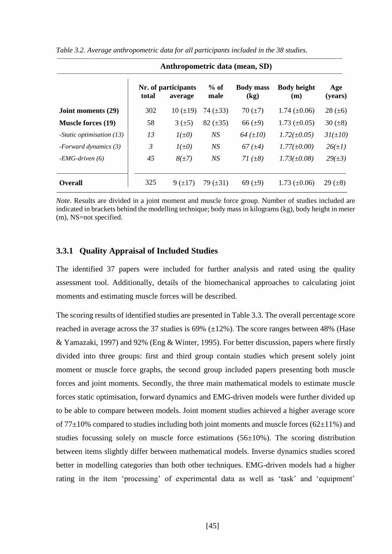
[45]

Table 3.2. Average anthropometric data for all participants included in the 38 studies.

Anthropometric data (mean, SD)

Nr. of participants total average

% of

male Body mass

(kg) Body height

(m) Age

(years)

Joint moments (29) 302 10 (±19) 74 (±33) 70 (±7) 1.74 (±0.06) 28 (±6)

Muscle forces (19) 58 3 (±5) 82 (±35) 66 (±9) 1.73 (±0.05) 30 (±8)

-Static optimisation (13) 13 1(±0) NS 64 (±10) 1.72(±0.05) 31(±10)

-Forward dynamics (3) 3 1(±0) NS 67 (±4) 1.77(±0.00) 26(±1)

-EMG-driven (6) 45 8(±7) NS 71 (±8) 1.73(±0.08) 29(±3)

Overall 325 9 (±17) 79 (±31) 69 (±9) 1.73 (±0.06) 29 (±8)

Note. Results are divided in a joint moment and muscle force group. Number of studies included are

indicated in brackets behind the modelling technique; body mass in kilograms (kg), body height in meter

(m), NS=not specified.

3.3.1 Quality Appraisal of Included Studies

The identified 37 papers were included for further analysis and rated using the quality

assessment tool. Additionally, details of the biomechanical approaches to calculating joint

moments and estimating muscle forces will be described.

The scoring results of identified studies are presented in Table 3.3. The overall percentage score

reached in average across the 37 studies is 69% (±12%). The score ranges between 48% (Hase

& Yamazaki, 1997) and 92% (Eng & Winter, 1995). For better discussion, papers where firstly

divided into three groups: first and third group contain studies which present solely joint

moment or muscle force graphs, the second group included papers presenting both muscle

forces and joint moments. Secondly, the three main mathematical models to estimate muscle

forces static optimisation, forward dynamics and EMG-driven models were further divided up

to be able to compare between models. Joint moment studies achieved a higher average score

of 77±10% compared to studies including both joint moments and muscle forces (62±11%) and

studies focussing solely on muscle force estimations (56±10%). The scoring distribution

between items slightly differ between mathematical models. Inverse dynamics studies scored

better in modelling categories than both other techniques. EMG-driven models had a higher

rating in the item ‘processing’ of experimental data as well as ‘task’ and ‘equipment’

[46]

description. Forward dynamics rated worse than EMG-driven and inverse dynamics studies,

especially for items ‘task’, ‘equipment’, and ‘EMG’.

The overall average scoring across items was distributed between 43 and 100%. ‘Aim’ reached

the highest score, as this had been clearly stated in all of the studies and, therefore, scored 100%.

A high score was also achieved for ‘discussion’ which focused on the rating of the graphical or

numerical analysis as well as the inclusion of description of limitations and conclusion. The

item with the poorest rating was data ‘processing’ where eleven studies did not state any

information about the processing tool used. The validation of the chosen mathematical models

was not always included. Seven studies gave no information about any validation process

whatsoever. Four studies used validation data extracted from other studies and sources, for

example EMG signals (Table 3.4).

Three criteria describing the modelling techniques were included in the quality assessment tool

(kinematic, kinetic and muscle modelling) which showed differences in their scoring results.

The ‘kinetic modelling’ criterion was rated similar between different mathematical model

groups (average values between 63-71%); the ‘kinematic modelling’, however, ranged between

55% (kinematic modelling of muscle force studies) and 76% (kinematic modelling of joint

moment studies) and showed a wider distribution throughout the papers. Compared to both of

these criteria, ‘muscle models’ were scored higher, with an overall average of 98% and the

lowest score of 80%.

Both ‘validation’ and ‘EMG’ items were only applied for studies estimating muscle forces.

Muscle force estimations in pure muscle force modelling papers were poorly validated and

often compared against EMG excitations from external literature (e.g., Komura & Nagano,

2004). In average, these papers were scored with 38%. Better ratings were achieved by papers

presenting both joint moments and muscle forces, with an average score of 64%. The item

‘EMG’ was rated in average with 69% and 53% for muscle force studies and studies including

both inverse dynamics and muscle forces, respectively. The papers often did not state the type

of filter used for the EMG signals or cut-off frequency. Only Buchanan and colleagues (2005)

stated all required information.

[47]

Table 3.3. Studies which are included into the scoring process and their scoring results.

Note. 1=static optimisation, ²=EMG-driven models, ³=forward dynamics.

[48]

Table 3.3. Continued.

Note. 1=static optimisation, ²=EMG-driven models, ³=forward dynamics.

[49]

3.3.2 Measurement Equipment and Data Processing

A range of measurement equipment has been used to collect experimental data (Table 3.4).

Most studies used optoelectronic motion analysis capture systems of Vicon (n=11) to capture

kinematic trajectory marker data. Koopman and colleagues (1995) used goniometers on the hip,

knee and ankle to measure joint kinematics, two electrical foot contact switches under both feet

defined the timing of initial contact and toe off. Eight studies have not specified which motion

system they have used to collect kinematic data. The number of cameras used ranged between

three and 22, with a measurement frequency between 50 and 500Hz.

All studies combined motion capture systems with force plates or pressure insoles to generate

the input data needed for the muscle force estimation process. The ground reaction forces were

either captured through a strain gauge system (AMTI, Bertec, Kyowa) or through a piezo-

electronic system (Kistler). One study, however, used pressure insoles to capture the ground

reaction forces (Faber, Kingma, Martin Schepers, Veltink, & van Dieen, 2010). Faber and

colleagues (2010) used shoes provided with 3D force sensors beneath the heel and the forefoot

and sampled at 50Hz. The measure frequency ranged between 60 and 2400Hz.

Three out of five studies which applied EMG data in their models used fine wire electrodes:

two with bipolar 50µm wire electrodes but with an unknown system (Bogey, Gitter, & Barnes,

2010; Bogey et al., 2005). The third study (Buchanan et al., 2005) captured one muscle (soleus)

with fine wire, whereas the other muscles were captured with surface electrodes (Noraxon

9000). No specific information about the fine wire electrode was given. Other studies used

surface EMG electrodes. Heintz and Gutierrez-Farewik (2007) captured with Motion Lab

System electrodes and White and Winter (1993) with a customised 16-channel PPM-FM

telemetry unit. In general, the measurement frequency for EMG signals ranged between 500 to

2500Hz.

A wide range of different processing protocols have been applied in identified studies. The

processing and filtering of experimental data is not always fully stated, sometimes even not

mentioned at all. In general, kinematic data are filtered with a low pass 2nd (n=2) or 4th (n=13)

order Butterworth filter which a cut-off frequency between 2 and 10Hz. Ganley and colleagues

(2004) used a Woltring routine with an estimated mean square error of 20mm. Similar

techniques in processing data can be found for the processing of ground reaction forces, where

the range of the low pass filter lies between 2 and 60Hz.

[50]

Both studies from Bogey and colleagues do not specify the post-processing filtering of the EMG

signals but define a rectification and integration through a moving integration scheme. The

other three studies including EMG used following filter: low pass 8Hz cut-off 4th order

Butterworth (Buchanan et al., 2005), high pass 20Hz cut-off 10th order Butterworth and low

pass 5Hz cut-off 3nd Butterworth (Heintz & Gutierrez-Farewik, 2007), and low pass 2Hz cut-

off 2nd order Butterworth filter (White & Winter, 1993).

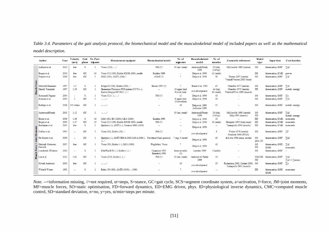
[51]

Table 3.4. Parameters of the gait analysis protocol, the biomechanical model and the musculoskeletal model of included papers as well as the mathematical

model description.

Note. --=information missing, //=not required, st=steps, S=stance, GC=gait cycle, SCS=segment coordinate system, a=activation, f=force, JM=joint moments,

MF=muscle forces, SO=static optimisation, FD=forward dynamics, ED=EMG driven, phys. ID=physiological inverse dynamics, CMC=computed muscle

control, SD=standard deviation, n=no, y=yes, st/min=steps per minute.

[52]

Table 3.4. Continued.

Note. --=information missing, //=not required, st=steps, S=stance, GC=gait cycle, SCS=segment coordinate system, a=activation, f=force, JM=joint moments,

MF=muscle forces, SO=static optimisation, FD=forward dynamics, ED=EMG driven, phys. ID=physiological inverse dynamics, CMC=computed muscle

control, SD=standard deviation, n=no, y=yes, st/min=steps per minute.

[53]

3.3.3 Biomechanical Models

As defined in chapter II the biomechanical model simplifies the complex human anatomy to

define segments and joints in a way it can be applied into kinematic and kinetic calculations.

Most of the studies included a reasonable description of the biomechanical model they have

implemented (Table 3.3). In majority of the cases, the bony structure of the lower limbs was

divided up into seven different segments, pelvis, left and right thigh, left and right shank, and

left and right foot, linked together with a three-degrees-of-freedom joint over a fixed joint centre

(Baker, 2013). This organisation of the bones and joints, called the Conventional Gait Model

(Baker, 2013), is represented by most of the studies and can be found in studies referring to

Kadaba and colleagues (Kadaba et al., 1989) and to the PlugInGait system of Vicon. Some of

the studies using the Vicon motion system did not directly refer to the PlugInGait model,

however, the description about the marker model suggests the use of the PlugInGait model.

An alternative to the Conventional Gait Model are six degrees of freedom models which assume

the segments are unconstrained at joints. Most such models used the Cleveland Clinic Protocol,

which was applied in the Motion Analysis Corporation’s Orthotrack software (Baker, 2013),

and the Calibrated Anatomical System Technique which was presented by Cappozzo and

colleagues (1995). A six DoF system called LAMB was used from one of the studies (Table 3.4)

which was developed (Laboratory for the Analysis of Movement in Children) from Rabuffetti

and Crenna (2004) and two others used that of Vaughan and colleagues (1992).

For 11 out of 38 studies it was not possible to identify the type of biomechanical model. Glitsch

and Baumann (1997) referred to an abstract from Baroni et al. presented on the XVth

International Congress Biomechanics 2004. However, the abstract was not found to be able to

confirm the biomechanical model used. Same problem occurred with the paper of Kerrigan and

colleagues (1998) referring to a supplement from Pedotti and Frigo in Functional Neurology

from 1992, and with Liu and Lockhart (2006) who referred to a study which has no additional

information about the biomechanical model.

3.3.4 Musculoskeletal Models

The musculoskeletal model to estimate muscle forces describes the segments’ and muscles’

properties as well as the definition of the passive structures if included into a model (e.g. tendon,

ligaments). Most musculoskeletal models found in identified studies are derived from the model

[54]

of Delp and colleagues (Delp, 1990; Delp et al., 1990). The basic model of one leg consists of

seven rigid segments (pelvis, femur, patella, tibia/fibula, talus, foot, toes) with 43

musculotendon actuators attached to bony landmarks which were defined by digitising human

bones.

These actuators were Hill-type muscle models, adapted from Zajac’s work (1989), and scaled

in its maximum isometric force, the optimal-muscle fibre length, the pennation angle of the

muscle, and the tendon slack length (see also chapter II). The information of these scaling

factors were derived from Wickiewicz and colleagues (1983) and Friedrich and Brand (1990).

Most papers using the model of Delp adjusted the number of segments or the number of muscle

tendon actuators depending on their focus of the study. Some included an upper limb model

(Table 3.4) mostly by one segment representing the head arms and trunk (HAT) or additional

segments at the foot.

Three of the identified studies refer to the musculoskeletal model of Anderson and Pandy (1999)

which is modelled as a 10-segment (HAT, pelvis, left and right thigh, left and right shank, left

and right hind- and forefoot) 23 degree of freedom linked model actuated by 54 muscle tendon

muscles (24 muscles per leg). Muscle-tendon paths were adapted from the Delp model, the

dynamics of the muscle-tendon unit from Zajac (1989). The model of Anderson and Pandy also

allows to include ligaments into the model which are represented by joint torques restricting

the joints in their range of motion. For all three studies there were no adjustments made

regarding the number of segments or musculoskeletal actuators.

Six studies developed their own models (Table 3.4). They differ in the number of muscle-tendon

actuators and in the number of segments. However, the muscles were mostly modelled based

on the Hill-type muscle model. Hase and Yamazaki (1997) defined a full body 19 segments,156

muscle model which all joints modelled as ball joints. Collins (1995) modelled only in two

dimensions using seven segments and eight muscles spanning the hip, knee, and ankle. Leardini

and O’Conner (2002) focused only on the ankle joint which was modelled as a one degree of

freedom hinge joint spanned by the tibialis anterior, the soleus and the gastrocnemius including

three extensor retinaculum bands. Silva and Ambrosio (2003) defined 35 muscle actuators for

one lower extremity with 16 segments of a full body model which are used to present a new

solution to solve the redundant problem with mathematical modelling. The model of White and

Winter (1993) was not fully described in their study as the number of muscles used for

modelling and simulation are missing. The model is based on a classical seven segment

[55]

approach. Fluit and colleagues (2012) used the simulation tool AnyBody to implement a model

into their estimation which has been developed in the Sim Mechanics toolbox of Simulink

(MatLab 7.11.0, The MathWorks). Six segments are included but the number of muscles is not

defined. However, this study only focused on the calculation of joint moments and not the

estimation of individual muscle forces and was, therefore, only included in the joint moments

group.

3.3.5 Sources of Geometric Parameters

The biomechanical models which are used for experimental data collection as well as the

musculoskeletal models have to be scaled according to the subject specific anthropometric data.

For the bony segments this means that the mass, the centre of gravity, and the moment of inertia

are adjusted accordingly (Vaughan, Davis, & O'Connor, 1999). The values are either taken from

cadaver studies, are calculated by mathematical models, are estimated by using different scan

systems (e.g., magnetic resonance imaging), or can be measured by kinematic data (Table 3.4).

Identified studies often refer to cadaver studies from Dempster (1955) or Chandler and

colleagues (1975) for the inertia and the bony mass of the segments. Another study referenced

widely is the technical note from de Leva (1996) who adjusted the values of Zatsiorsky and

colleagues (1990). Zatsiorsky estimated body segment’s inertial parameters with a gamma-ray

scanner of 100 male undergraduate students. Another study which was used in some of the

studies is that from Havanan (1964) who used a mathematical model to estimate the inertial

properties. The model needs 25 different dimensions of the whole body to be able to scale the

model which includes the circumference of the ankle, knee, thigh, head, or the foot length as

well as the chest depth. With the further knowledge of the body mass Havanan set calculations

for every segment with which it is then possible to estimate the anthropometrics of the body

segments.

Another reference for body segment scaling is the work of McConville (1980). They used a

technique called stereophotometrics which implements a three dimensional photography of the

participant by cameras placed around the participant. Specific coordinates of body points serve

as input into calculations which reconstruct the participant. McConville used this method to

determine the relationship between the body anthropometrics and its body segments mass

distribution on living participants.

[56]

3.3.6 Mathematical Modelling Techniques

Three main mathematical modelling techniques which estimated muscle forces were identified

across the 19 included studies: static optimisation, an inverse dynamics approach (thirteen

studies), forward dynamics and EMG-driven models, two dynamic optimisation approaches

(three and six studies).

Static optimisation solves the redundancy problem (more muscles spanning a joint than degrees

of freedom exist) by dividing up the experimental joint moments in different muscle forces

acting on that joint at each independent instant in time. In other words, this method does not

optimise the estimation by considering the whole time period of a gait cycle as a whole but

analysis the muscle forces for each time step with only the experimental input given for this

time step. The information of the joint kinematics as well as the calculated joint moments lets

the model search for the optimal muscle activations, considering for example the moment arm

of the muscles as well as the muscle characteristics defined in the musculoskeletal model while

solving the equation of motions of the skeletal system (derived from the Newtonian mechanics,

in more detail in chapter 4.4). Output are the muscle activations as well as muscle forces at each

instance in time, without taking the activation-contraction cycle into account.

Forward dynamics instead matches the desired kinematics with estimated kinematics by using

generalised muscle excitations and experimental ground reaction forces which is solved time-

dependent over the whole gait cycle. This means, that forward dynamics computes a set of

muscle excitations by solving the equation of motions, representing the electrical stimulation

arriving at the muscle, and with the information of the ground reaction forces drives the model

in time forward. This results in the kinematics of the next time step which are then compared

the experimental kinematics, while the error between estimated and experimental kinematics

are minimised. Therefore, one time step might influence the results of the whole gait cycle as

forward dynamics optimises the outcome of this whole time period. To be able to do so, this

technique needs additional information like the activation-contraction cycle of the muscle

(chapter 2.6.1) which enables the model to output individual muscle forces (chapter 4.4).

EMG-driven models are another dynamic optimisation approach. Instead of the computed

muscle excitations, EMG-driven models use experimental EMG excitations as input in the

estimations. This constrains the muscles of the model regarding their level of activation

throughout the gait cycle. With this information, the model can then estimate joint moments or

powers which are then compared and their error minimised to the experimental data. Two

[57]

studies presented an enhanced inverse dynamics approach called physiological inverse

dynamics (De Groote et al., 2009) and computed muscle control (Lin et al., 2012), both

including additionally the activation-contraction cycle to a standard static optimisation

approach (for more information, please see Chapter VI).

Both static optimisation and forward dynamics models use different optimisation functions to

overcome the redundancy problem (Table 3.4). These functions normally minimise a cost

function, which in the case of identified studies are the sum of squared muscle activations, the

sum of all muscle forces or the sum of (squared) muscle stress. Forward dynamics can use

additionally cost functions which are time depended, for example the minimisation of the

metabolic energy. This is an advantage for patients with diseases affecting the activation-

contraction coupling like neurological disorders.

3.3.7 Validation of Estimated Muscle Forces

A direct validation of estimated muscle forces is only possible with in-vivo techniques.

However, good quality EMG data can give first indications about when a muscle should be

active. Twelve of the 19 muscle modelling studies compared their estimated muscle forces with

EMG patterns. In most cases, on-off pattern of the muscle activity were presented and not a

whole activation of EMG excitations. The researchers rarely captured EMG data on their own

participants and used EMG patterns found in the literature. Only three studies compared the

muscle force estimation to experimental EMG data that they had captured themselves. The other

studies which used EMG as a validation tool included EMG excitations from Inman (1953),

Perry (1992), Hof (2002), or Anderson and Pandy (2001b). Leardini and O’Connor (2002) do

not state their source of EMG patters they use in their graph as a validation.

Another validation process is the comparison of joint moments received through the muscle

force estimation process with a classical static optimisation approach using ground reaction

forces. Two EMG-driven studies used experimental joint moments for the validation process

(Bogey et al., 2005; Buchanan et al., 2005). A variation of this technique is shown in the second

study of Bogey and colleagues (2010) who used the ankle power as a comparison. In total, four

studies did not validate their muscle force estimations at all.

[58]

3.3.8 Outcome Measures

Overall, joint moments of the hip, knee and ankle in sagittal, frontal, and transverse plane were

present and were included in the digitising process. Figure 3.4 to Figure 3.7 and Figure 3.8 to

Figure 3.15 present single curves as well as the grand mean and one and two standard deviation

bands of the joint moments and muscle forces, respectively.

Estimated force data was available for 19 individual muscles or muscle groups: gluteus

maximus, medius and minimus, psoas and iliacus (or iliopsoas), rectus femoris, vastus lateralis,

medialis and intermedius (or vastii), semitendinosus, semimembranosus, biceps femoris long

head and short head (or hamstrings), tensor fasciae latae, gastrocnemius lateralis, medialis,

soleus (or triceps surae), tibialis anterior, and tibialis posterior. These muscles are all

responsible for the process of walking (M. Q. Liu, Anderson, Pandy, & Delp, 2006; Perry &

Burnfield, 2010). As described in the method section, muscles were summed up if identified

studies divided muscles into different compartments. This has been done for the iliopsoas

(psoas, illiacus), vastii (medialis, lateralis), gastrocnemius (medialis, lateralis), and the

hamstrings (semitendinosus, semimembranosus, biceps femoris long head. Number of studies

presenting joint moments and muscle forces which are included into the digitising progress are

listed in Table 3.5 and Table 3.6.

Table 3.5. Number of studies which present joint moments of the lower limb divided up in hip, knee and

ankle in sagittal, frontal and transverse plane.

Joint moment sagittal frontal transverse

Hip 19 9 7

Knee 20 6 5

Ankle 27 8 8

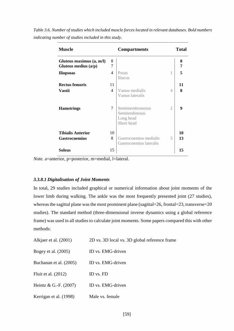
[59]

Table 3.6. Number of studies which included muscle forces located in relevant databases. Bold numbers

indicating number of studies included in this study.

Muscle Compartments Total

Gluteus maximus (a, m/l)

Gluteus medius (a/p) 8 7

8 7

Iliopsoas 4 Psoas

Iliacus 1

5

Rectus femoris 11 11

Vastii 4 Vastus medialis

Vastus lateralis 4

8

Hamstrings 7 Semimembranosus

Semitendinosus Long head

Short head

2

9

Tibialis Anterior 10 10

Gastrocnemius 8 Gastrocnemius medialis

Gastrocnemius lateralis 5 13

Soleus 15 15

Note. a=anterior, p=posterior, m=medial, l=lateral.

3.3.8.1 Digitalisation of Joint Moments

In total, 29 studies included graphical or numerical information about joint moments of the

lower limb during walking. The ankle was the most frequently presented joint (27 studies),

whereas the sagittal plane was the most prominent plane (sagittal=26, frontal=23, transverse=20

studies). The standard method (three-dimensional inverse dynamics using a global reference

frame) was used in all studies to calculate joint moments. Some papers compared this with other

methods:

Alkjaer et al. (2001) 2D vs. 3D local vs. 3D global reference frame

Bogey et al. (2005) ID vs. EMG-driven

Buchanan et al. (2005) ID vs. EMG-driven

Fluit et al. (2012) ID vs. FD

Heintz & G.-F. (2007) ID vs. EMG-driven

Kerrigan et al. (1998) Male vs. female

[60]

Lin et al. (2012) ID vs. SO vs. CMC vs. FD

Liu et al. (2006) 3D local vs. 3D global

Ren et al. (2008) Force plates vs. only kinematic data to calculate joint moments

Schache et al. (2007) Different reference frames

White et al. (1993) ID vs. EMG-driven

The female and male joint moment curves from Kerrigan showed significant differences at the

knee flexion moment in pre-swing after being normalised to body mass and height. Therefore,

gender curves were averaged together before they were included in the calculation of the overall

mean and standard deviation. For all other studies, only the standard approach inverse dynamics

to calculate joint moments was included into the digitising process as this will give the

opportunity to compare the consistency between this standard approach to the new developed

models to estimate muscle forces. Single curves of extracted joint moments can be found in

Figure 3.4 which are all presented as internal moments.

[61]

Figure 3.4. Mean joint moment profiles extracted from each identified study.

[62]

In the following paragraphs, averaged lower limb joint moment profiles are presented through

a grand mean and one and two standard deviation bands over the whole gait cycle normalised

to the body mass and height. All studies were ensemble averaged up to 60% of the gait cycle

and is represented by a straight line in figures below. Only those providing swing phase

information are presented after. Numbers in brackets indicate the number of studies included in

the graph. Table 3.7 summarises the peak values of the grand mean as well as the CV of peak

values.

Table 3.7. Maximum and minimum of averaged joint moments across included studies including

standard deviation (SD) and coefficient of variation (CV) normalised to body mass and height. Number

of joint moment profiles included are defined in brackets.

Joint Moment Maximum

(N*m/kg*m) SD CV

GC

(%)

Minimum (N*m/kg*m)

SD CV GC

(%)

Hip sagittal (19) 0.38 0.23 0.6 3 -0.46 0.17 0.4 50

0.18 0.12 0.7 96

frontal (9) 0.48 0.14 0.3 15 0.26 0.08 0.3 31

0.45 0.10 0.2 45

transverse (7) 0.09 0.03 0.3 12 -0.07 0.03 0.5 48

Knee Sagittal (20) 0.35 0.16 0.4 14 -0.12 0.05 0.4 42

0.12 0.08 0.7 56 -0.13 0.05 0.4 95

Frontal (6) 0.29 0.18 0.6 13 0.11 0.05 0.5 32

0.22 0.11 0.5 46

Transverse (5) 0.04 0.02 0.4 9 -0.06 0.06 0.5 50

Ankle Sagittal (27) 0.82 0.12 0.1 48 -0.10 0.07 0.7 5

Frontal (8) -0.08 0.05 0.7 51

Transverse (8) 0.09 0.06 0.4 46

Hip joint moments

Sagittal hip joint moments were presented in 19 studies (Figure 3.5). Highest CV was found at

the end of swing (96%) with 0.7, however, with a much smaller mean value than both other

peak moments. The two other peaks experienced slightly smaller CVs. Fontal and transverse

joint moments, included in nine and seven studies, respectively, reached CV values up to 0.5

with the smallest CV of 0.2 at the second peak. The highest standard deviations are mostly

found close to the peak values and generally in stance. Highest moments on the hip is shown

[63]

for the hip abduction moment. Almost all studies included the full gait cycle for the hip joint

moments, except three studies (Alkjaer et al., 2001; DeVita, 2005; J. Liu & Lockhart, 2006).

Knee joint moments

Knee joint moments are presented in Figure 3.6. 20 studies included knee joint moments in the

sagittal plane, while five of them focused on the stance phase only. Knee abduction and knee

rotation moments were less present in the identified studies with six and five, respectively. The

highest standard deviation at the knee extensor moment occurred during the first peak at 14%

of the gait cycle. Here, the CV is the smallest at the knee with a CV of 0.4. A CV of 0.4 was

also reached at the minimum peak in the sagittal plane as well as one peak in transverse plane.

Highest CV occurred on the second maxima at the knee extensor moment (0.7), however, as

well with a much smaller mean than other moment peaks sagittal at the knee.

Highest standard deviation bands are present for knee abduction moments in stance. The

standard deviation stays high across stance but is the highest close to the peak moments. All

three knee moments tend to go against zero in swing phase and also show small standard

deviation bands. The highest peak is shown for the knee extensor moments with 0.388N/kg,

whereas the smallest is shown in transverse plane for the knee rotation moment.

Ankle joint moments

27 studies included the plantar flexor moments, while eight studies concentrated on the stance

phase only (Figure 3.7). For the frontal and sagittal plane, there are more studies including the

stance phase only than the full gait cycle. All three joint moments at the ankle are close to zero

in swing, whereas the standard deviation bands stay close to zero, too.

The CVs lie between 0.1 and 0.7, whereas the highest CVs occurred in the sagittal and frontal

plane on the smaller peaks in stance. The standard deviation band in the sagittal plane is quite

consistent throughout the stance phase. The highest joint moment throughout all joint moments

is the ankle plantarflexor moment with at least two times higher moments than on the knee or

hip. Ankle inversion and rotation moments are quite small compared to the other moments.

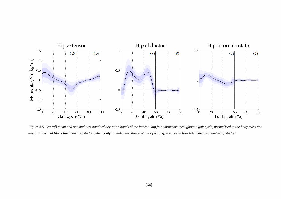
[64]

Figure 3.5. Overall mean and one and two standard deviation bands of the internal hip joint moments throughout a gait cycle, normalised to the body mass and

–height. Vertical black line indicates studies which only included the stance phase of waling, number in brackets indicates number of studies.

[65]

Figure 3.6. Overall mean and one and two standard deviation bands of the internal knee joint moments throughout a gait cycle, normalised to the body mass

and –height. Vertical black line indicates studies which only included the stance phase of waling, number in brackets indicates number of studies.

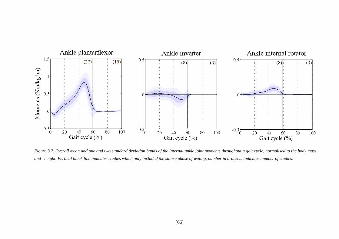
[66]

Figure 3.7. Overall mean and one and two standard deviation bands of the internal ankle joint moments throughout a gait cycle, normalised to the body mass

and –height. Vertical black line indicates studies which only included the stance phase of waling, number in brackets indicates number of studies.

[67]

3.3.8.2 Digitalisation of Muscle Forces

The following section describes the muscle forces of tibialis anterior, gastrocnemius, soleus,

rectus femoris, vastii, hamstrings, iliopsoas, gluteus maximus and gluteus medius across a gait

cycle. The muscle forces were synthesised in three groups according to the model on which

they were derived: static optimisation (SO), forward dynamics (FD) or EMG-driven models.

The following studies included more than one mathematical model to estimate muscle forces

and their graphical presentations were divided up according to the mathematical model used:

Anderson& Pandy (2001b) SO physiological vs SO non-physiological vs FD

De Groote et al. (2009) classical inverse approach vs physiological inverse approach

Heintz& G.-F. (2007) SO vs EMG-driven

Lin et al. (2012) SO vs CMC vs FD

Silva& Ambrosio (2003) Two different SO types

The average across the gait cycle was taken for the two static optimisation approaches from

Silva and Ambrosio (2003) and from Anderson and Pandy (2001b) as these pattern all represent

an inverse dynamic approach. The three main mathematical models (static optimisation,

forward dynamics, EMG-driven models) have been included in the digitalisation process,

however, the physiological inverse approach from De Groote and colleagues (2009) as well as

the mathematical model called computed muscle control form Lin and colleagues (2012) were

neglected due to rare presence in the literature. They are, thus, discussed further in the

discussion section below.

Individual profiles of muscle forces extracted out of identified studies can be found in Figure

3.8. In general, different studies show large variations between each other, however, for most

of the muscles a broad agreement exists on an overall force pattern. Considerable variability

can be found in minor features like smaller peaks or in magnitude. The consistency between

studies seem to vary across different muscles; while studies of the hamstrings or the

gastrocnemius are quite similar in their activation patterns and magnitudes, muscles like the

iliopsoas or the tibialis anterior have distinctive differences in shape and magnitude between

studies. Several muscles show evidence of different patterns in sub-sets of the studies especially

[68]

at gluteus maximus where two different patterns at initial contact and early stance exist. This

seems not dependent on modelling approaches as both static optimisation and forward

dynamics are included into both force sub-sets which suggests that other factors may be more

important for differences between studies. Contrary to this, EMG-driven force patterns have

mostly smaller force generations throughout the gait cycle than forward dynamics.

For some of the muscles and specific parts of the gait cycle, clear outlier can be detected. The

study of Lin and colleagues (2012) (iliopsoas and gluteus medius, both static optimisation and

forward dynamics), of Hase and Yamazaki (1997) (rectus femoris, forward dynamics), of

Ackland and colleagues (2012) (hamstrings, static optimisation), of Heintz and Gutierrez-

Farewik (2007) (rectus femoris, EMG-driven) and the study of Komura and colleagues (2005)

(vastii and gastrocnemius, static optimisation) show a much higher and/or longer maximal force

development than remaining studies. Other muscle force patterns like the iliopsoas from

Fraysse and colleagues (2009) (static optimisation), the soleus and the tibialis anterior of Heintz

and Gutierrez-Farewik (2007) (EMG-driven), the soleus of Anderson and Pandy (2001b) (static

optimisation and forward dynamics) or the tibialis anterior of Glitsch and colleagues (1997)

(static optimisation) show total different patterns than the rest of the studies. The results of Lin

and colleagues and Anderson and Pandy suggest as well that other factors than the principles

behind the mathematical models to estimate muscle forces may be influencing the differences

between studies.

The most outstanding curve which has been extracted from identified studies is the hamstring

estimation from Fraysse and colleagues (2009). This profile shows a completely different

pattern than the rest of extracted hamstrings profiles. While other studies present the hamstrings

to be active in the beginning of the stance phase and at the end of swing, the curve of Fraysse

and colleagues has its maximum in mid-stance while being inactive at the start and in the end

of the gait cycle. Because this pattern is totally contradictive to known EMG excitation studies,

too (Perry & Burnfield, 2010; Winter, 1990), the hamstring profile of Fraysee and colleagues

has been excluded.

[69]

Figure 3.8. Single muscle force profiles normalised to the body mass (N/kg), extracted out of identified studies. Blue=static optimisation, red=forward dynamics,

green=EMG-driven models.

[70]

Table 3.8 describes maximum peak forces and their CVs as well as the maximal standard

deviation across a gait cycle, split up into different mathematical model groups. They are further

described in the following paragraphs which give an overview about digitised muscle force

profiles of the lower limb. Across all muscle forces, static optimisation is the most frequently

used technique compared to forward dynamics and EMG-driven models. No EMG-driven

model has been used to estimate muscles on the hip joint (iliopsoas, gluteus maximus and

medius).

Table 3.8. Maximal standard deviation and maximal peak force of the lower limb muscles, normalised

to the body mass. Number in brackets indicate number of muscle profiles included.

Muscle type max 1 SD CV GC (%) max 2 SD CV GC (%)

Tibialis anterior SO (7) 5.56 4.34 0.8 6 2.64 1.66 0.6 96

FD (1) 1.14 -- -- 64 -- -- -- --

EMG-dr. (3) 2.98 2.79 0.9 4 2.81 1.00 0.4 78

Gastrocnemius SO (10) 15.08 7.46 0.5 44

FD (2) 12.35 0.95 0.1 45

EMG-dr. (5) 13.53 2.88 0.2 46

Soleus SO (11) 20.03 9.67 0.5 47

FD (2) 23.12 1.58 0.1 48

EMG-dr. (5) 16.55 7.78 0.5 46

Rectus femoris SO (8) 2.71 1.58 0.6 21 4.22 2.39 0.6 54

FD (3) 2.35 2.82 1.2 10 5.86 7.78 1.3 51

EMG-dr. (3) 1.72 1.37 0.8 12 1.86 -- -- 63

Vastii SO (7) 13.71 9.91 0.7 12 3.07 2.41 0.8 62

FD (2) 14.07 3.39 0.2 12 5.17 0.81 0.2 62

EMG-dr. (2) 10.27 7.02 0.7 13 -- -- -- --

Hamstrings SO (7) 6.78 5.79 0.9 2 4.57 1.71 0.4 94

FD (2) 4.02 2.44 0.6 2 3.46 0.72 0.2 94

EMG-dr. (2) 4.05 2.55 0.6 2 -- -- -- --

Iliopsoas SO (5) 7.17 7.93 1.1 48

FD (3) 8.97 12.55 1.4 50

EMG-dr. (-) -- -- -- -- -- -- -- --

Gluteus max SO (6) 4.21 3.67 0.9 12

FD (4) 4.75 4.87 1 12

EMG-dr. (-) -- -- -- -- -- -- -- --

Gluteus med SO (7) 10.60 15.04 1.4 14

FD (2) 27.94 26.36 0.9 12

EMG-dr. (-) -- -- -- -- -- -- -- --

Note. GC=gait cycle, SD=standard deviation, CV=coefficient of variation, EMG-dr.=EMG-driven.

[71]

Tibialis anterior

Ten studies included the tibialis anterior (eleven curves), whereas only one study used forward

dynamics. There is considerable variability between studies estimating tibialis anterior force

generation (Figure 3.8). In most cases, studies suggest peak activity in early stance but show

considerable variation on the magnitude. Most also suggest activation in swing which is lower

and also shows considerable variability in magnitude. Collated data (Figure 3.9) from both

static optimisation and EMG-driven analyses confirms activation in late swing rising to a peak

in first double support (6% gait cycle) but high SD and CV confirm considerable variability

concerning the magnitude of these peaks. Force generation is low in second half of stance. EMG

driven studies show increased activation in the first half of swing (peaking at 78% gait cycle

with reasonably good repeatability) which is not present in any of the static optimisation studies.

Data from the one forward dynamics study is quite different to the other two with minimal force

generation in stance but a low level of activation through swing.

Soleus

With 18 curves extracted out of 15 studies, soleus is the most frequently estimated muscle.

There exist a considerable variability between studies in magnitude and timing of maximal

muscle force production (Figure 3.8). Peak forces lie between 30 and 60% of the gait cycle and

are about 10 to 40N/kg high. Except one study (EMG-driven model of Heintz & Gutierrez-

Farewik, 2007), studies suggest no force development in swing. Averaged profiles confirm

maximum forces to be around 50% with high SD bands and CVs showing a high variability

between studies (Figure 3.10). Averaged maximum force from all three mathematical models

are similar in timing and magnitude. EMG-driven in swing phase and forward dynamics at first

double support (8%) show different patterns compared to static optimisation which may be

triggered through outliers described above. Forward dynamics CV is much smaller than for

static optimisation or EMG-driven models which is confirmed through the standard deviation

bands.

Gastrocnemius

17 curves from 13 studies define the muscle forces progression of the gastrocnemius during

walking. There exists a general agreement between studies about the activation profile (Figure

[72]

3.8). After forces stay close to zero until 10-15% of the gait cycle, studies suggest a rise in force

up to 50% of the gait cycle leading onto a rapid fall down close to zero at about 60% of the gait

cycle. At initial foot contact and at the end of swing studies agree in a small force development.

Considerable differences are shown in the magnitude of the maximum muscle force which lies

around 10 to 30 N/kg. Peak forces and profiles are similar between mathematical models

(Figure 3.11). The standard deviation for static optimisation is much higher than for forward

dynamics and EMG-driven curves. Static optimisation and forward dynamics show the same

patterns of late swing phase force generation which is completely lacking with EMG-driven

models. Static optimisation’s CV is as for the soleus much greater than for forward dynamics,

but also for EMG-driven approaches.

[73]

Figure 3.9. Overall mean and one and two standard deviation bands of the tibialis anterior throughout a gait cycle, normalised to the body mass, divided up

into three mathematical models static optimisation., EMG-driven, and forward dynamics. Vertical black line indicates studies which only included the stance

phase of walking, number in brackets indicates number of studies.

[74]

Figure 3.10. Overall mean and one and two standard deviation bands of the soleus throughout a gait cycle, normalised to the body mass, divided up into three

mathematical models static optimisation., EMG-driven, and forward dynamics. Vertical black line indicates studies which only included the stance phase of

walking, number in brackets indicates number of studies.

[75]

Figure 3.11. Overall mean and one and two standard deviation bands of the gastrocnemius throughout a gait cycle, normalised to the body mass, divided up



[76]

Hamstrings

Nine studies included muscle force estimations of the hamstrings (eleven curves). There is

considerable consistency in profile and magnitude between these studies estimating hamstrings

force production except for the force magnitude during initial contact (Figure 3.8). At this point

of the gait cycle studies suggest a peak activation which decreases to zero at 20% of the gait

cycle. After this first maximum hamstrings’ forces stay close to zero until mid-swing at 80% of

the gait cycle when the second maximum appears (90-95% of the gait cycle). Two slight

different patterns are shown at the second maximum peak by two static optimisation curves

being different to the rest of the curves (Collins, 1995; Rodrigo, Ambrósio, Tavares da Silva,

& Penisi, 2008). First maximum peak between EMG-driven and forward dynamic approaches

are similar with high standard deviation bands and CVs (Figure 3.12). Static optimisation shows

here a greater maximum as well as higher standard deviation bands and CVs which, however,

may result out of the heavy influence of one outlier (Ackland et al., 2012). Static optimisation

and forward dynamics agree in the force production during swing but with a higher standard

deviation and CV for static optimisation; EMG-driven models did not include the swing phase.

Rectus femoris

Recuts femoris has been presented in eleven studies which included in total 14 curves. There

exists considerable variability between studies in rectus femoris force pattern and magnitude

(Figure 3.8). An overall agreement is suggested by two peak forces during the first half of stance

and during the second half of stance with decreasing force in swing down to zero. Static

optimisation and forward dynamics suggest overall similar patterns with a small difference at

the end of swing (Figure 3.13). Big differences in variability exist due to higher standard

deviation bands and CVs for forward dynamics during the second peak. These differences may

occur through the highly influence of one outlier (Hase & Yamazaki, 1997). EMG-driven

analyses are different compared to others between 40-100% of the gait cycle. In this part of the

gait cycle, the second peak does not occur and a constant force production in swing exists which

is not shown for static optimisation and forward dynamics. However, only one study has

estimated rectus femoris forces during swing with an EMG-driven approach which may

represent the force production of an outlier (Heintz & Gutierrez-Farewik, 2007).

[77]

Vastii

Graphical presentation of eleven curves have been detected in eight studies presenting the

muscle force generation of the vastii muscle group. There exists an overall agreement in the

pattern of vastii muscle forces but with high variability in magnitude for the maximum peak at

10-15% of the gait cycle (Figure 3.8). Second smaller peak occurs at transition from stance to

swing. Between first and second peak as well as after the second peak until the end of swing

studies suggest minimal forces close to zero, except two outliers (Heintz & Gutierrez-Farewik,

2007; Komura et al., 2005). These may be responsible for the difference in force pattern and

variability between mathematical models (Figure 3.14). Static optimisation and forward

dynamics show similar patterns but different CVs during the first maximum peak. Furthermore,

there exists different standard deviations between static optimisation and forward dynamics

during the swing phase caused through the static optimisation outlier of Komura and colleagues

(Table 3.8). Forward dynamics shows a steep peak force development at about 10% of the gait

cycle, which reflects the heavy influence of the curve of Anderson and Pandy (2001b).

Compared to static optimisation and forward dynamics, EMG-driven analyses present one

curve with a different pattern during the swing phase which reflects the pattern of the outlier of

Hientz and Gutierrez-Farewik (Figure 3.8). Both outliers cause the higher standard deviation

bands for static optimisation and EMG-driven approaches compared to forward dynamics

(Table 3.8).

[78]

Figure 3.12. Overall mean and one and two standard deviation bands of the hamstrings throughout a gait cycle, normalised to the body mass, divided up into

three mathematical models static optimisation., EMG-driven, and forward dynamics. Vertical black line indicates studies which only included the stance phase

of walking, number in brackets indicates number of studies.

[79]

Figure 3.13. Overall mean and one and two standard deviation bands of the rectus femoris throughout a gait cycle, normalised to the body mass, divided up



[80]

Figure 3.14. Overall mean and one and two standard deviation bands of the vastii throughout a gait cycle, normalised to the body mass, divided up into three

mathematical models static optimisation., EMG-driven, and forward dynamics. Vertical black line indicates studies which only included the stance phase of

walking, number in brackets indicates number of studies.

[81]

Iliopsoas

As described above, all three hip muscles (iliopsoas, gluteus maximus and medius) have not

been included in an EMG-driven approach. Five studies and eight force profile curves in total

presented the force production of the iliopsoas during walking. All curves included the whole

gait cycle. Figure 3.8 shows very poor agreement between studies. Shapes in force production

as well as magnitudes differs greatly between studies. The averaged curves in Figure 3.15

presenting static optimisation and forward dynamics are similar in shape and magnitude but

seem heavily influenced through two outliers from Lin and colleagues (2012). After a small

force generation during initial contact the force rises up to 50% of the gait cycle where it

decreases again to a smaller force similar to forces appearing during initial contact. Throughout

the gait cycle, high standard deviation bands exist which maximise around peak force and

represent the great variability between curves. Both mathematical models have CVs over 1

(Table 3.8).

Gluteus maximus

Ten curves showing the gluteus maximus forces could be extracted which were presented in

eight studies. The studies suggest two sub-sets in shape during initial contact until 40% of the

gait cycle (Figure 3.8). One sub-set has a peak force close to initial contact which quickly

decreases close to zero until 20% of the gait cycle, whereas the other pattern shows small forces

during initial foot contact, which rises to its maximum at 20% of the gait cycle and decreases

again until 40% of the gait cycle. Both sub-groups have curves from both static optimisation

and forward dynamics. Studies suggest as well a small force production of the gluteus maximus

close to zero except two studies which are slightly activated until the end of swing (Hase &

Yamazaki, 1997; Lin et al., 2012). Both outliers, however, are not from the same sub-group.

The average force profile of mathematical models is similar between each other. The slight

difference of the forward dynamics curve of Hase and colleagues at the end of swing is

represented through a small differences between the average profiles of static optimisation and

forward dynamics. Standard deviation bands and CVs are similar between mathematical models

(Table 3.8).

[82]

Gluteus medius

Seven studies with nine curves in total have been extracted showing the gluteus medius force

generation. A considerable variability between studies is shown, whereas two different sub-sets

can be defined (Figure 3.8). One sub-group, however, are two curves from the same study (Lin

et al., 2012). This study shows a high peak at 18% of the gait cycle, and a decrease up to 40%

with a second small peak at 50% of of the the gait cycle, whereas other studies are in general

agreement with each other showing a slow rise in force to a much smaller force between 20-

50% of the gait cycle compared to the curves of Lin and colleagues. Except the forward

dynamics curve of Lin and colleagues, studies agree in a small force until the end of swing.

Averaged curves of static optimisation and forward dynamics show similar patterns but great

differences in magnitude for the peak at about 15% of the gait cycle. This may represent the

outliers of Lin and colleagues and a different number of other studies of the second sub-group

with which they are combined to form the average force profile (Figure 3.15). This also may be

reflected in the higher standard deviations and CV of forward dynamics compared to static

optimisation (Table 3.8).

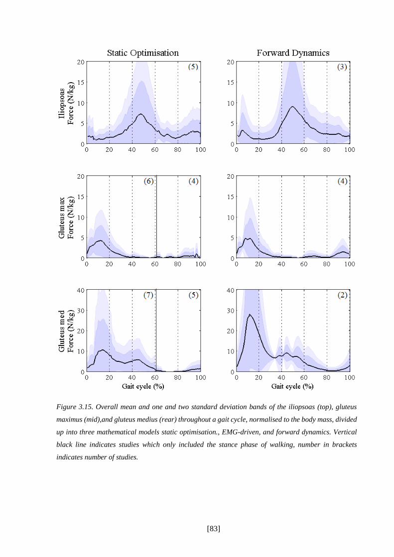
[83]

Figure 3.15. Overall mean and one and two standard deviation bands of the iliopsoas (top), gluteus

maximus (mid),and gluteus medius (rear) throughout a gait cycle, normalised to the body mass, divided

up into three mathematical models static optimisation., EMG-driven, and forward dynamics. Vertical

black line indicates studies which only included the stance phase of walking, number in brackets

indicates number of studies.

[84]

3.4 Discussion

This systematic review aimed to analyse existing estimated muscle force profiles of the lower

limb during human healthy walking which were published in the academic literature. The

objective was to be able to analyse the state-of-the-art of musculoskeletal modelling related to

walking, to define the best mathematical method for the clinical gait analysis routine and to

formulate recommendations for a standardised protocol. Joint moment profiles were included

in the systematic review, too, which serve as a comparison in variability as well as a first

indicator for the quality of the muscle force estimations.

The systematic review identified 9870 studies through initial electronic screening of relevant

databases resulting in a much higher number than in comparable earlier reviews (e.g., Hollands,

Pelton, Tyson, Hollands, & van Vliet, 2012; McGinley et al., 2009; Peters et al., 2010;

Ridgewell et al., 2010, between 374 and 1132 studies). The cause for this may be that this

systematic review is a “sensitive” rather than a “selective” search. This is driven by the need to

identify a small number of studies which can be described using a wide variety of terms

covering multiple research areas.

The results between joint moments and muscle force studies differ in their quality reporting and

numerical or graphical moment and force presentation. A first quality distinction between

muscle force and joint moment studies was made through the scoring principle. Studies

focussing solely on the estimation of joint moments had a 20% higher overall score (77±10%)

in comparison to muscle force studies (56±10%). Muscle force studies reached a smaller rating

especially in the items ‘task’ description and ‘measurement equipment’ compared to joint

moment studies. This may be due to a different interest of muscle force modelling studies as

they often focus solely on the presentation of their mathematical model and underlying

processes, which is reflected by a high rating of item ‘muscle models’. The focus on the

practical and clinical details seems often secondary. However, experimental data collection is

crucial and should be presented in more detail. Joint moment studies, on the other side, are

mostly based on a clinical background or focus on parameters related to the experimental data

processing.

The quality assessment tool showed an overall higher score for EMG-driven models estimating

muscle forces than static optimisation and, especially, forward dynamics. Forward dynamics

papers scored worse than both other techniques in all items except ’muscle models’, ‘validation’

and ‘discussion’. Especially studies involving forward dynamics are focused on the description

[85]

of the musculoskeletal model and scored lower in other items. EMG-driven models scored

higher in items related to the experimental data collection but showed deficits in presenting

other items. All three modelling techniques have, therefore, significant limitations in presenting

and describing the techniques and protocols they have used but inverse dynamics and EMG-

driven models are achieving overall better results than forward dynamics. These scores,

however, do not reflect the quality of the actual research of the studies. Missing information

make it harder to compare the quality between studies and mathematical models with each

other.

Another difference between joint moments and muscle force studies were the number of

participants involved. Studies analysing joint moments included in average more participants

than muscle force studies (10±19 vs 3±5, respectively). Most mathematical modelling studies

estimating muscle forces included only a single participant (n=16 out of 19 studies). This may

result of the fact that these studies simply presented their model technique on one participant

(e.g., Anderson & Pandy, 2001b). Only three EMG-driven studies presented more than one

participant (Besier, Fredericson, Gold, Beaupre, & Delp, 2009; Bogey et al., 2010; Bogey et

al., 2005). In some studies, although more than one participant has been included, only one

representative participant has been numerical or graphical presented (e.g., Ganley & Powers,

2004). To be able to include mathematical modelling into a clinical gait analysis routine,

adequate data of a normative population is needed. To date, however, such a data pool has not

been published.

3.4.1 Joint Moments and Muscle Force Profiles

Individual joint moment profiles are in broad agreement with each other. The pattern across a

gait cycle is in general similar between studies, except the ankle joint moment in the frontal

plane. This may occur because of the different foot models used across studies (Ferrari et al.,

2008). This shape similarity between joint moment profiles is not present for the muscle forces

which resulted in considerable differences between studies. A general agreement exists during

maximum peak forces, however, with different levels of agreement for different muscles. For

some of the muscle peak forces, the on-off pattern is similar but the force peak is shifted, for

example the soleus where the peak forces of individual studies can be found between 30-60%

of the gait cycle. The results of the CVs confirm a higher consistency for joint moments than

for muscle forces, although the CV distribution between muscles is not homogenous. Most CVs

[86]

for joint moment peaks are saying under 0.5. For muscle force peaks, however, the CV range

from 0.1 up to 1.4. Especially muscles acting on the hip (iliopsoas, gluteus maximus and

medius) reach CV values over 1. Two muscles experience smaller CVs which are the soleus

and gastrocnemius on the shank.

Distinctive outliers or sub-groups were detected for almost all muscle forces. Sub-groups were,

however, not dependent on mathematical models. Individual outliers came from eight different

studies which included curves of all three different mathematical models. For almost all of these

studies, only one of their presented muscle was detected as an outlier; all other estimated muscle

forces were in the range or had no abnormal force profile compared to the others. Quality

assessment analysis results of studies including these outliers ranged from very low to high

quality scores. Other possible factors which may have affected the outliers to be different to the

others, may be the mathematical model or the cost function for optimisation. However, studies

with outliers vary between all these factors, which may suggest a multifactorial influence on

the estimation of muscle forces. As not all studies have reported clear information about their

experimental data collection it may also result out of different protocols and poor experimental

data.

The process of muscle force prediction can be simply divided in two main parts, the

experimental protocol and its data as well as the actual modelling and simulation process. This

“decoupling” of the experimental and modelling/simulation part is useful as different factors

may influence the outcome of muscle force estimation. These are defined in the following

chapters.

3.4.1.1 Influences on the Output through the Experimental Protocol and Data

Variability in joint moments and muscle force profiles may occur because of different reasons

affecting the experimental data. A change in magnitude around a peak moment or peak force

may occur because of different walking speeds (Schwartz et al., 2008). Schwarz and colleagues

(2008) and Lelas and colleagues (2003) analysed the dependence of speed on kinematics,

kinetics, and EMG excitations and show that speed has a significant influence on these

parameters and that especially peak values increased or decreased with walking speed. This

may be also partially the case for time shifts as the stance-to-swing relation changes with

walking speed (Schwartz et al., 2008).

[87]

Other factors related to experimental data collection may have influenced the differences

between studies. The filtering of experimental data which has been undertaken before the data

was used in the calculations to receive joint moments and muscle forces could have influenced

the output. For example the cut off frequency has an influence on the kinematics data which is

used for both inverse dynamics and muscle force estimation as an input (Sinclair, Taylor, &

Hobbs, 2013). But also the filtering of the ground reaction force could have changed the

estimations’ output (van den Bogert & De Koning, 1996). The reference frame in which

moments referring to may change the kinematics as well (J. Liu & Lockhart, 2006; Schache,

Baker, & Vaughan, 2007). Finally, the applied biomechanical model contains parameters which

influence the calculation of kinematics and kinetics. Ferrari and colleagues (2008) compared

five different biomechanical protocols with each other, including the PlugInGait model, the

LAMB model and the CAST model (6-degree-of-freedom model). They placed 60 markers on

three participants so that they were able to use the same trials for comparison. There result

showed that (although intra-protocol variability was small) inter-protocol variability revealed

high variability between protocols. Especially in the frontal and transverse plane the

correlations were poor for the knee and ankle. The authors conclude, that comparing results

from different protocols should be carefully undertaken.

Interestingly, one of the studies which was excluded from this systematic review compared the

influence of different body segments’ parameter estimation techniques, including the model of

Havanan, the cadaver studies from Dempster and Chandler, and the in vivo body mass scan

technique from Zatsiorski and colleagues and de Leva (Rao, Amarantini, Berton, & Favier,

2006). They observed that when applied to the classical gait analysis the body segment

parameters were highly sensitive to the different techniques applied and received great

differences during the swing phase. Furthermore, the study from Ren and colleagues (2008)

claims that the mass properties of body segments can affect the estimated joint forces and

moments. On top of this, a third study from Ganley and colleagues (2004) focused on lower

limb anthropometry and compared a method using dual energy X-ray absorptiometry with the

values of Chandler’s work. They concluded that especially in swing phase joint moments could

be influenced by using different anthropometric measures as the ground reaction force is zero.

[88]

3.4.1.2 Influences on the Output through Modelling and Simulation Processes

The higher consistency of joint moment profiles compared to profiles of estimated muscle

forces may indicate that irregularities between muscle force estimations may not only result out

of differences in experimental input but also through other factors related to the mathematical

muscle force modelling and simulation. Three main mathematical models were identified (static

optimisation, forward dynamics, EMG-driven). In general, no mathematical method has been

found to result in more consistent results than others. Static optimisation was the most

frequently applied method compared to the others and often used as a reference model to

compare to other mathematical models. Static optimisation seems to be seen as the most widely

accepted approach in the literature.

Some differences were detected in the magnitude of the peaks as well as some steeper or flatter

rise in force production. Particular the profiles of forward dynamics experienced quite steep

force developments which even could reach discontinuities (e.g., vastii). In some cases the

magnitude differs (e.g. the hamstrings). Additionally, smaller peaks occurred for some of the

muscles especially with forward dynamics which were not shown for the other mathematical

models. EMG-driven models stayed for some of the muscles active across the whole gait cycle

whereas other modelling techniques had phases where there was no force production at all.

Some identified studies compared mathematical models with each other. Anderson and

colleagues (2001b) compared static optimisation with forward dynamics during healthy

walking. They showed a general agreement between models, but some smaller differences for

some of the muscles could also be detected. They concluded that static and dynamic

optimisation should be seen as “complementary approaches”. However, their comparison may

have been biased by the fact that they used the joint moments estimated through the dynamic

optimisation technique as an input in the static optimisation pipeline.

Heintz and Gutierrez-Farewik (2007) compared a static optimisation approach with an EMG-

driven approach. The paper focused on the different energetic performance criteria while using

the sum of muscle stress squared in the static optimisation approach and the product of maximal

isometric muscle force in the EMG-driven approach. The maximal isometric forces used for

the definition of the muscles as well as to normalise EMG excitations were the same. Results

showed big differences between some of the muscles analysed. Lin and colleagues (2012)

compared a static optimisation approach with computed muscle control (CMC) and a forward

dynamics method adapted from Seth and Pandy (2007). Their results showed similar patterns

[89]

of muscle forces estimated by the three approaches for both walking and running in healthy

adults as well. However, the data is only based on one participant. Furthermore, they used two

different musculoskeletal models and simulation environments (Matlab and OpenSim) for

different mathematical approaches which may have influenced the simulations’ output. To

verify both musculoskeletal models they run static optimisation though both simulation

environments. Although an overall similarity could be shown some differences in magnitude

and shape between both static optimisation solutions can especially be seen for muscles on the

thigh and hip.

These results of Lin et al. have shown that using two different musculoskeletal models in two

different simulation environments may change the estimation’s output. Ten of the 19 muscle

modelling studies used the musculoskeletal model of Delp and either applied it in the standard

version or changed the number of muscles or number of segments (Delp, 1990; Delp et al.,

1990). It is the model which is used regularly for muscle force modelling purposes in the

academic literature. Other musculoskeletal models applied in identified studies were for

example the musculoskeletal model developed by Anderson and Pandy (1999). However, as

described in chapter II, they implemented parts of the Delp model, especially the geometric

information for most of the muscles.

As discussed before, anthropometric differences and differences in the geometry of the

musculoskeletal model can lead to differences in the modelling output. The degrees-of freedom

of a model (Sartori, Reggiani, Farina, & Lloyd, 2012), the geometric properties of the segments,

the number of the muscles, the geometries of the muscles, and the activation-contractions of

the muscle-tendon properties influence the calculations’ outcome. Although the Delp model

has been used in more than 50% of the studies it has been adapted to the needs of the studies

which may have led as well to the inconsistency between studies. Body segments parameters

like the segments’ mass or inertia and the source of lower limb anthropometry may also

influence the estimations’ outcome (Ganley & Powers, 2004; Rao et al., 2006; Ren et al., 2008).

Some studies model muscles as one single line, whereas others represent a muscle by more than

one compartment, especially when muscles fulfil more than one task. For example the gluteus

maximus is a wide muscle which is involved with the extension, adduction and rotation of the

leg. One of the developed models of Delp and colleagues (1990) represents this muscle with

three different compartments.

[90]

Another factor which could have influenced the output of muscle force estimations are the

different cost functions which were applied in identified studies. Monaco and colleagues (2011)

changed the exponent of the muscle power from n=2 up to n=100 and compared their results to

surface EMG excitations. They concluded that the exponent factor can have a significant

influence on the final results. Collins (Collins, 1995) compared different optimisation

techniques with each other, including the minimisation of the total muscle force, the total

muscle force squared, total muscle stress, total ligament force, total contact force inter-articular,

and instantaneous muscle power. Their result showed differences between minimisation

principles and that the minimisation of total ligament force was the less successful method when

compared to surface EMG excitations.

3.4.1.3 Muscle Force Estimation Compared to Experimental EMG

Experimental EMG excitations can either be used as an input into the estimation of muscle

forces (EMG-driven models) or may be used as an indirect validation to get a first impression

about the validity of the estimated muscle forces. A limitation of many identified studies

estimating muscle forces was that, although muscle force studies frequently compared their

estimations against EMG excitations they often did not comment on differences between

mathematical model estimation and EMG or defined a “general agreement” between estimation

and EMG excitations. For example Anderson and Pandy (2001b) experienced a great jump in

their muscle force estimation of some of the muscles which they did not comment on in detail.

Rodrigo and colleagues (2008) presented a much earlier maximum peak using static

optimisation, still in the double support phase of the gait cycle, as the other studies show a burst

in the single support phase.

But not all studies were ignoring differences occurring between estimation and EMG excitation.

The EMG-driven estimation of Heintz and Gutierrez-Farewick (2007) shows the soleus

especially in swing a totally different pattern than all the other studies. They conclude that it

may indicate noise from the soleus’ EMG signal. They further discuss that differences may

result out of a failure to properly normalise the soleus to a known maximum force. They also

criticise surface EMG in general that especially in the swing phase EMG excitations may reduce

the quality of the estimation of muscle forces due to known limitations (electrical disturbances,

electrode misplacement, intra-subject variation).

[91]

To get a first indication about the validity of the averaged digitised curves of identified studies

they can be compared to the EMG excitations of Winter (1990). The patterns of averaged

muscle forces are in a general agreement with Winter’s EMG excitations. However,

mathematical models differ for some of the muscles. For example, muscle force estimations of

tibialis anterior are in their profile very similar to Winter’s work, however forward dynamics

shows a complete different activation in stance. Same results are found for the hamstrings,

where static optimisation and EMG-driven models have similar patterns to Winter’s EMG

excitations of medial and lateral hamstrings, but forward dynamics shows an additional small

activation around stance-to-swing transition which is not shown in Winter’s EMG work.

Gluteus maximus shows two different sub-sets of estimated muscle forces during the first 20%

of the gait cycle. Winter’s data supports the sub-set with the later peak, however, different sub-

sets may also indicate different activation profiles between participants.

Extracted profiles from identified studies of the rectus femoris revealed interesting findings.

The studies mainly agree on a peak activation at about 50% of the gait cycle. However, Winter’s

EMG pattern shows two additionally peak forces at beginning and at the end of the gait cycle.

The study of Nene and colleagues (2004) investigated this behaviour and realised that these

additional activations are crosstalk from the vastii muscle group which are captured with

surface EMG equipment. They compared surface EMG to indwelling fine-wire EMG and could

show that rectus femoris is only active at about 50% of the gait cycle. This information is an

indication that the quality of the estimation of muscle forces may be good and that the

mathematical models do work. It is important that in cases where muscle forces have been

estimated with the help of EMG to careful interpret these results because of the known

limitations of EMG and the differences between excitation and force production of a muscle.

When comparing the results to Winter’s work the results show that not all outliers are totally

off the muscle activation pattern. For example the force estimation of the gluteus medius in Lin

and colleagues work shows a total different force profile than the other studies, but is the one

closest pattern to the EMG gluteus medius from Winter. However, most of the outliers differ to

the EMG activations of Winter, like the two outliers on the tibialis anterior. This shows the

broad variability between studies and the difficulty in defining the “correct” muscle force

estimation pattern. It is also important to keep in mind while comparing estimated muscle force

data to experimental EMG excitation that muscle forces are not equal to muscle excitations.

This means that although differences may exist between estimated muscle forces and

[92]

experimental EMG profiles that this is not a measurement or estimation error but simply the

natural differences between the excitation of the muscle and the latter muscle force production.

3.4.1.4 Recommendations for a Protocol Suitable for the Clinical Gait Analysis

Summarised, significant limitations were shown for all three mathematical models, but the

approach most promising for the clinical gait analysis is static optimisation as this method has

already been widely used and tested in the literature. Furthermore, the summarised data

presented in chapter 3.3 suggests that static optimisation produces results that are at least as

consistent as shown for the other modelling techniques. Also, this method is much more time

efficient compared to forward dynamic methods (Anderson & Pandy, 2001b) and is

independent of EMG measures. An advantage of static optimisation to the models using

experimental EMG excitations is the limitation of EMG-driven models reflected by the missing

estimated forces of muscle at the hip (e.g. iliopsoas, glutei) which shows the restrictive access

to specific muscles. Therefore, the robustness, its efficiency, the independence from

experimental EMG excitations, as well as the summarised results of the literature makes static

optimisation the most attractive model to be included into a clinical routine to estimate muscle

forces (Lin et al., 2012).

The limitation of this approach compared to the others is that it does not take the muscle

activation dynamics into account (Lin et al., 2012). This might be a limitation for patients with

disorders affecting the activation-contraction cycle. A new developed technique called

computed muscle control (CMC) which was presented in the identified study of Lin and

colleagues (2012) promises to keep the computational time low while including the activation-

contraction cycle by combining an inverse and a forward method. It was developed in

cooperation with two main research groups involved in musculoskeletal modelling (Thelen,

Anderson, & Delp, 2003) and is already implied in simulation environments like OpenSim.

This approach, however, has not yet been widely tested in the literature and needs detailed

testing and comparison with static optimisation.

Many influencing factors related to the experimental data collection or the modelling and

simulation process were detected. It is important to understand the influence of these factors to

be able to analyse estimated muscle forces. Known limitations resulting out of these factors can

be taken into account to be able to use muscle force estimation in a clinical environment.

However, more research needs to be undertaken to understand better the individual influences

[93]

of these factors. Also, to be able to compare between gait laboratories, it is either important to

know the different protocols and the resulting changes in muscle force estimation profiles, or a

standardised and free available protocol needs to be developed which can be used by every gait

laboratory.

The validation of estimated muscle forces is crucial, however, to date only indirect methods are

applicable in the clinic. Numerical or graphical presentation of muscle forces were often

indirectly validated with experimental EMG excitations. Frequently, however, studies used

EMG data from other studies or only compared to EMG on-off bars. Best validation with EMG

excitations are experimental data of the same participant and same trial which has been used

for the estimation of muscle forces. By doing so, individual differences as well as trial-to-trial

differences can be eliminated. This is also important for EMG-driven estimations of muscle

forces. It is crucial for these models to use high quality EMG excitations into the calculation of

these models as this data are used to define the activation pattern of a muscle. EMG-driven

models are, therefore, highly dependent on the operators knowledge and experience.

To be able to create a standardised and free available protocol a simulation tool needs to be

included which fulfil these needs. The simulation tool OpenSim is a free available tool in the

internet and already frequently used in the literature. This simulation environment has been also

used in one of the included studies (Lin et al., 2012). Some of the mathematical models provided

by OpenSim were already tested in the literature which makes this programme attractive to

include into a standardised protocol. OpenSim has some other advantages compared to other

programmes, which is that it gives access to detailed information about the musculoskeletal

models. Furthermore, it provides a pipeline called SimTrack which gives the operator the

possibility to estimate muscle forces in a routine processing (Delp et al., 2007). Also, the

musculoskeletal models are based on the model from Delp which has been used and tested

several times in the academic literature. Finally, it offers a wide range of different mathematical

models, including the classical inverse dynamics approach (static optimisation) and the new

developed technique CMC.

3.4.2 Limitations

Some limitations of this systematic review need to be discussed. To normalise the extracted

joint moments and muscle force graphs the averaged body mass and body height across all

included studies has been estimated to be used for studies which have not included this

[94]

information. This may have slightly altered the graphical presentation of joint moment and

muscle force profiles. Also the stance phase was normalised to 60% in relation to swing in case

this relation was not mentioned in the study. Another factor which may have influenced the

consistency of muscle force profiles are the different walking speeds of the participants in

identified studies (R.R. Neptune et al., 2008). Because not all studies mentioned the exact

walking speed it was not possible to normalise against speed.

Furthermore, the process of digitising caused some issues for some of the joint moment and

muscle force curves. Due to factors like the differences in the quality of colours, overlaying

curves, or the graphs’ differences in resolution, the digitising process could have caused some

inaccuracies. Overlying curves resulted in manual digitising and guessing of the right rack of

the curve, and different line widths, especially thick lines could have lead to errors. However,

it was always attempted to approach the middle of these lines when they needed to be manually

digitised.

[95]

3.5 Conclusion

This is the first study which thoughtfully summarised the knowledge about muscle force

estimation during walking. Also, it is the first time that experimental data from the literature

has been digitised and a huge amount of data has been merged together to be able to judge the

variability which exists in the literature regarding joint moments and muscle forces of the lower

limb in healthy adults.

Therefore, the results of the systematic review give a summary of what is known about muscle

force estimation during human normal walking in the academic literature. Joint moment profiles

were more consistent than muscle force profiles which showed that work needs to be done to

conduct a standardised protocol to estimate muscle forces to eliminate influencing factors which

may affects results. The well-established estimation of joint moments have been tested several

times in the academic literature which makes a clinical interpretation of these possible. Limiting

factors are known which can be taken into consideration. To be able to reach a similar standard

for muscle force estimations, limiting factors need to be tested. This needs to be done on more

than one participant to account for individual differences which may be otherwise interpreted

as indication for another influencing factor. Direct validation of the estimation of muscle forces

is not yet possible, however, the comparison to EMG excitation gives first indication when a

muscle should produce force.

This standardised protocol needs to close the gap between a classical engineering and clinical

approach. Both, the quality of the musculoskeletal model and the mathematical model to

estimate muscle forces needs to be tested but also the application and understanding in a clinical

setting needs to be given. According to the results of this systematic review, static optimisation

is the model most suitable for the clinical but new developed techniques like computed muscle

control may have potential to be used in the clinic, too. These models, however, need to be

tested and implemented into a classical gait analysis routine to be able to judge their potential

to be included into a standardised protocol. The dominance of OpenSim and its advantages

compared to other simulation tools make it attractive to be included in such a standardised

clinical routine. It provides the musculoskeletal models and mathematical approaches of

interest to estimate muscle forces while the operator can customise the models according to the

needs.

Therefore, the following chapter will test OpenSim’s potential to be included into a standardised

protocol using static optimisation and computed muscle control which then will be used in

[96]

praxis on a healthy population of ten participants. This will help to understand the clinical

evidence of the estimation of muscle forces and may provide additional steps to be undertaken

before the protocol can be used on patients in a clinical gait analysis routine.

[97]

CHAPTER IV

4 Technical Development of the Modelling and Simulation

Protocol

A standardised protocol for the clinical gait analysis which includes muscle force estimation

must be easy applicable and understandable. The systematic review has shown that to-date static

optimisation, an inverse dynamics approach, may be the mathematical model most suitable for

the clinic. Compared to forward dynamics or EMG-driven models it has a lower calculation

time, is independent of EMG, and more robust than forward dynamics. However, static

optimisation does not include the muscle activation-contraction dynamics in the estimation of

muscle forces. Other limitations of these models are that they are essentially an optimisation

technique optimising for example the overall muscle activation which may be not valid in

conditions with disrupted neurological control. However, these techniques are to-date the best

way which can be achieved to estimate muscle forces at the current state-of-the-art. The new

developed method computed muscle control (CMC) pledges to combine both a low

computational cost and the activation-contraction dynamics of the muscle. This technique has

not been widely tested but first results show promising results (Lin et al., 2012) with potential

advantages. Therefore, additional to static optimisation CMC is proposed to be tested for the

use in clinical gait analysis.

To estimate muscle forces as a part of routine clinical gait analysis a simulation tool which can

be incorporated into routine data processing is required. OpenSim is a freely available

simulation tool which incorporates both static optimisation and CMC. The operator has the

possibility to modify parameters in the musculoskeletal model OpenSim is supplied with or to

create their own musculoskeletal model. One of the OpenSim models, gait2392, is the most

frequently used in the literature to analyse muscle forces in the lower limb during walking and

seems the most suitable model for this study (chapter III). Another advantage of OpenSim is

that it provides additionally a standardised pipeline called SimTrack with, which the kinematics

and kinetics as well as muscle forces can be estimated. At the start of this PhD project,

OpenSim’s SimTrack pipeline was planned to be used as a tool in its standard configuration

while applying the musculoskeletal model gait2392 in its standard form. After running some

[98]

pilot studies it became clear, however, that some minor and major adjustments were required

to make the protocol suited to the requirements of clinical gait analysis.

This chapter, thus, describes the simulation tool OpenSim and its musculoskeletal model

gait2392 and the SimTrack pipeline and how these have been adapted in the light of these

requirements. The standard package is described first followed by a number of separate

adaptations that were undertaken. In the end a standardised protocol for gait analysis which

includes the estimation of muscle forces during walking will be proposed which will be tested

in the following chapter (chapter V).

[99]

4.1 Introduction to OpenSim

OpenSim is a simulation tool already frequently used in various research fields. OpenSim arose

out of SIMM (Software for Interactive Musculoskeletal Modelling), a commercial tool which

is used for biomechanical modelling, surgical planning, and ergonomic analysis (Delp et al.,

2007). With SIMM it has been possible to create, alter, and evaluate different models of a wide

range of musculoskeletal structures which have then been used to simulate different

movements. Some are walking, running, cycling or stair climbing, or the consequences of

different surgical implementations in joint mechanics or muscle function (R. R. Neptune &

Hull, 1999; R. R. Neptune, Kautz, & Zajac, 2001; Thelen & Anderson, 2006; Thelen et al.,

2005). SIMM, however, is essentially a modelling package and has very limited support for the

simulation of movement using those models. Particular disadvantage is that it does not provide

any assistance with the computation of muscle excitations for coordinated movements and only

limited tools to analyse the estimated results (Delp et al., 2007). On top of that, the user does

not have full access to the source code, which leads to difficulties in developing the researcher’s

skills and reproduce results achieved by other laboratories. As a consequence, OpenSim was

developed by Delp and colleagues (2007) as an open source project allowing operators full

access to all codes and models and incorporating a repository for the sharing of newly

developed code and models.

The OpenSim programme is, therefore, a free simulation tool with which it is possible to create,

exchange and analyse mathematical models and dynamic simulations of different kind of

movements (Delp et al., 2007). The core is programmed in C++, the graphical user interface

(GUI) is written in Java (Hicks, 2013). The first version 1.0 was presented at the American

Society of Biomechanics Conference in 2007. Since then, the programme has been used by

many researcher and scientists based in different research fields, including sport science,

computer animation, biomechanics research, robotics research medical device design,

orthopaedics, and many more (Arch et al., 2015; Holloway et al., 2015; Miller Buffinton,

Buffinton, Bieryla, & Pratt, 2016; Skalshoi et al., 2015).

The systematic review of this PhD has shown that OpenSim is already in use for the analysis

of human walking. Besides different other models which are applicable for a variety of body

parts involved in different movements, developed and shared either through the OpenSim group

or developed by other users, OpenSim provides also musculoskeletal models for the purpose of

human gait analysis. Because of its features OpenSim has, therefore, been chosen for this study

[100]

to estimate muscle forces during walking compared to experimental surface EMG which is

described in chapter V.

[101]

4.2 Musculoskeletal Model gait2392

Most of the models which are available in OpenSim are based on the musculoskeletal model of

Delp and colleagues (Delp, 1990; Delp et al., 1990). This model, in turn, was based on a model

developed at the VA Rehabilitation R&D Centre on Palo Alto, California, and includes 43

muscle-tendon actuators of the lower limb. Delp enhanced the model and developed a graphics-

based lower limb model to study the results of the musculoskeletal reconstructions on the

function of muscles and resulting movement. It can be used for surgery simulations to enable

an analysis and sttimation of surgical reconstructions of the muscles and bones of the lower

limb.

Since then, the model has been widely used for different purposes and has been tested and

adapted to present variations at a range of anatomical locations. For example Delp and Maloney

(1993) changed the hip centre position to analyse the effect on the capacity of the muscles of

generating forces and moments. They concluded that maximal muscle forces and moments are

sensitive to the location of the hip joint centre. Another study from Gonzales and colleagues

(1997) analysed the influence of muscle architecture and moment arms on the wrist flexion-

extension moments. The motivation of the work was to study the different contributions of

single muscles which span the wrist and to overcome the redundancy problem with this

simulation. One of the first publications in a human walking related study involving the Delp

model was from Piazza and Delp (1996), who analysed the role of muscles on sagittal knee

flexion during the swing phase of walking. In the same year Delp and colleagues (1996) studied

the length of the hamstrings and psoas during crouch gait in cerebral palsy compared to normal

walking and discussed the implications for a muscle-tendon surgery.

In OpenSim, musculoskeletal models are defined in an .osim file format using eXtended Mark-

up Language (XML). It is essentially a collection of rigid segments (bones) which are linked

by joints with a range of different degrees-of-freedom. Muscles are defined as acting in a

straight line between an origin on one segment and insertion on another. In some cases,

intermediate via points are included to represent wrapping around other structures like bones,

other muscles or retinacula. A model of the physiology of the muscles’ excitation, activation,

and contraction is incorporated to define the forces the muscles generate in response to a given

neurological impulse. Each of the different components is described by a number of parameters

(e.g., maximum isometric force, position of a joint centre, axial orientation…) which can be

modified by the user. Lower limb models also generally include a representation of how the

[102]

foot interacts with the ground (Hicks, 2012b). For the purpose of gait analysis a model including

the lower limb and the torso is mainly sufficient while considering the aim of the study. For a

standard gait analysis with interest on the lower limb no upper extremities are needed, as it has

been shown that the arm swing has a small influence on walking parameters (Umberger, 2008).

However, for some of the models a torso segment is included which presents to upper body

mass and is required for some of the calculations to estimate muscle forces.

The most frequently used model for gait simulations in OpenSim is a three-dimensional model

called gait2392, one of the core models in OpenSim. It has been adopted from the Delp model

(1990) and was designed for simulations of movements which are leg dominated (Au & Dunne,

2012). Main developers of the model were Darryl Thelen from the University of Wisconsin-

Madison and Ajay Seth, Frank C. Anderson and Scott L. Delp from the University of Stanford.

This model represents the segments torso (including the head), pelvis, femur, tibia, fibula, talus,

foot (including calcaneus, navicular, cuboid, cuneiforms, metatarsals) and toes (Figure 4.1).

Figure 4.1. OpenSim’s musculoskeletal model gait2392, with twelve segments, 23 degrees of freedom

and 92 muscle-tendon actuators.

[103]

The name of the model gives the degrees of freedom (23) and the number of muscle-tendon

actuators (92) of the model. The actuators can be summed up to 72 muscles, as some of the

larger muscles are represented through more than one muscle-tendon compartment depending

on their anatomy. For example, if a muscle is widely diversified and acts in more than one

direction like the gluteus then it may be modelled as a number of essentially independent muscle

elements (Figure 4.2). More information and a list of all actuators can be found in appendix A1.

Figure 4.2. Representation of the gluteus maximus in the OpenSim model gait2392. Three musculo-

tendon compartments define the whole muscle.

The generic model of gait2392 describes a male subject with a body height of 1.80m and a body

mass of 75.16kg. The bone geometry data of the pelvis and the femur are acquired by marking

the surface of bones with a mesh of polygons which were then digitised to determine the

coordinates of the vertices (Delp, 1990). Geometry data for the bones of the shank and the foot

have been adopted from a Master thesis of D.L. Stredney from the Ohio State University from

1982 (Au & Dunne, 2012). These coordinates of the bones are then used in a file to set the bone

geometries for the musculoskeletal model.

All segments are modelled as rigid-bodies, with each corresponding reference frame fixed

inside each segment (Figure 4.3). The axes are defined as x-axis to represent the anterior-

posterior direction, y-axis the proximal-distal direction, and z-axis the medio-lateral direction.

This stays constant for all reference frames and coordinate systems in this study. The relative

motion of the segments to each other are defined by the following joints: lumbar joint, hip,

knee, ankle, subtalar, and metatarsophalangeal (MTP) joint (Delp et al., 1990). The coordinate

frame of the pelvis is modelled parallel to the ground midway between the anterior superior

iliac spines (ASIS), meaning that in neutral position there exists a zero pelvic tilt with respect

[104]

to the laboratory’s ground. This is important to take into consideration, because many

biomechanical models used in clinical gait analysis use the pelvic tilt in neutral position (i.e.

location of ASIS and PSIS) as a zero reference and this is thus anteriorly tilted by an average

of 14° with respect to the gait2392 pelvis.

The length of the segments of the generic model gait2392 were extracted from Delp’s model

(1990). The anthropometric details of the segments including the mass and inertial properties

are adapted from Anderson and Pandy’s work (1999), who modelled a 10-segment, 23 degree-

of-freedom model. They based the inertial properties as well as the mass of the segments on the

average anthropometric data from five healthy participants (26 ± 3 age, 1.77 ± 0.03m, 70.1 ±

7.8kg) using the method of McConville (1980). For the model gait2392 these properties are

then multiplied by a factor of 1.05626 (Au & Dunne, 2012) which is defined in the OpenSim

user guide. This number, however, has not been verified by the developers of OpenSim and

reasons for the scaling to this factor are unclear. The centre of mass and inertia characteristics

for the hindfoot and the toes have been found by measuring the surface of a tennis shoe size 10

(Au & Dunne, 2012). The density is then divided up in separate foot segments while assuming

a uniform density of the foot with 1.1 g/cm3. All mass and inertial properties of the gait2392

model can be found in appendix A2.

Figure 4.3. Coordinate frames and centre of mass for each segment of the gait2392 model in OpenSim.

Red lines represents the x-axis, yellow lines represent the y-axis, and black lines represent the z-axis.

[105]

The characteristics of the lumbar joint are taken from the work of Anderson and Pandy (1999).

The trunk segment is articulated with the pelvis through a three degree-of-freedom ball and

socket joint which is located at the third lumbar vertebra. The hip joint is characterised as the

same type of joint as the trunk-pelvis joint, the femur head is fixed in the acetabulum of the

pelvis, whereas no translations between segments are possible.

The modelling of the knee joint is more complicated than the hip joint due to its multi-bone and

ligament structure. The knee joint properties are implemented from Yamaguchi and Zajac

(1989). They designed a one-degree of freedom model which includes both the tibio-femoral

and the patella-femoral joint. Additionally, it accounts for the levering mechanism of the

patellar. For the model gait2392 the patellar has been excluded to simplify the kinematic

constraints. The femoral condyles, modelled as ellipses, can move on the tibia plateau, with the

contact point of being a function of the knee angle (Nisell, Németh, & Ohlsén, 1986). Examples

of the segmental parameters defined in the .osim file of the gait2392 model can be found in

appending A3.

4.2.1 Muscle-tendon Properties

The geometry for the 92 muscle-tendon actuators from model gait2392 are, firstly, adapted

from the Delp model, who specified 43 muscles of one leg, and, secondly, from the work of

Anderson and colleagues’ model (Anderson & Pandy, 1999, 2001a) from which six of the

lumbar muscles were included. The lines of action of the muscles are defined using the

anatomical landmarks of the bony segments of the model (Anderson & Pandy, 1999; Au &

Dunne, 2012; Delp, 1990). These are represented either by one or more line segments called

actuators of the muscles. Mostly, the definition of the muscle’s origin and insertion is sufficient

to describe the line of action. However for some muscles, especially muscles spanning over

more than one joint or muscles which wrap over a bone (e.g., the muscles of the quadriceps) a

single line segment would lead to a wrong muscle path which might pass though the bones and

deeper muscles at specific angles of the joint (Delp et al., 1990). Therefore, intermediate via

points are included to prevent this happening (see chapter II).

Both the musculoskeletal model of Delp (1990) and Anderson and Pandy (1999) define the

muscle-tendon units with a Hill model type (Figure 4.4). The muscle fibres are modelled as a

[106]

contractile element (CE) in parallel with an elastic element (parallel elastic element, PE) which

represents all passive structures in and around the muscle. These are arranged in series with the

series elastic element (SE) which represents the tendon. Each muscle-tendon actuator is

characterised by a number of five parameters listed in the gait2392 .osim file.

Figure 4.4. Graphical presentation of the Hill-type muscle tendon model adapted from Thelen et al.

(2003) dividing the musculotendon complex into a contractile element (CE) and two elastic elements

PE and SE. The elastic elements are parallel to the CE (PE) and in series with the CE (SE).

Three of these parameters describe the muscle, the muscle maximum isometric force, the

optimal muscle-fibre length and the pennation angle to account for specific muscle

characteristics. The maximum isometric force of each muscle has been adapted from the Delp

model and has been calculated from the muscle’s measured cross-sectional area (Spector,

Gardiner, Zernicke, Roy, & Edgerton, 1980). It is assumed that the cross-sectional area and the

muscle volume are constant throughout the movement (Hoy, Zajac, & Gordon, 1990). The

cross-sectional area values have been taken from Friederich and Brand (1990) and Wickiewicz

and colleagues (1983). The maximal isometric forces stated in the ground work of Delp and

colleagues (1990) were scaled according to a specific individual factor, as the developers while

designing the gait2392 model, realised that the Delp model was too weak (Au & Dunne, 2012).

Appendix A1 defines the maximum isometric forces of all included muscles in gait2392.

The optimal muscle fibre length defines the length of the muscle fibre at which it can generate

the greatest force in isometric condition. Values describing the optimal muscle-fibre length and

the pennation angle of the muscle have been taken from the work of Wickiewicz and colleagues

(1983) and Friederich and Brand (1990). The values have been scaled with a factor of 2.8/2.2,

as 2.2μm are the initial values of the study but 2.8μm is the actual length of a sarcomere at

[107]

which the fibres can produce maximum force according to the sliding filament theory (Gordon,

Huxley, & Julian, 1966).

The other two parameters describe the tendon. The tendon elasticity has an effect on the muscle

force generation, which has been recognised by Hill (1938). The tendon can store energy while

being extended either actively through a concentric muscle contraction or passively by eccentric

movement. However, when Delp designed his model no experimental data existed about the

characteristics of the tendon length; the knowledge about the length of the tendon at which it

starts to store energy when stretched (tendon slack length) was missing. The solution was to

estimate the tendon slack length for each muscle-tendon actuator accounting for the optimal

muscle fibre length and the joint angle at which the muscle-tendon unit can generate the most

force in isometric contraction. Detailed description can be found in the dissertation of Delp

(Delp).

OpenSim provides a number of different muscle models which define the activation-dynamics

parameters of the muscle-tendon units. The standard model implemented in the gait2392 model

is the Thelen 2003 Muscle Model (Thelen, 2003). Three curves define parts of the individual

characteristics of the muscle-tendon units (Figure 4.5) which are the active and passive force-

length and force-velocity relationships of the muscle and the normalised force-length

relationship of the tendon.

Figure 4.5. a) Gaussian curve showing a muscle force-length relationship, normalised to the maximal

isometric force of the muscle and the optimal fibre length; b) Muscle force-velocity relationship, a

describing the activation of the muscle; c) Tendon force-strain relationship; adapted from Thelen (2003)

who refers to Zajac (1989).

[108]

Muscle force production starts with the innervation of the muscle fibres. The neural excitation

represents the firing rate of motor units which innervate the muscle tissue and causes the

calcium release from the sarcoplasmic reticulum. The muscle activation represents the calcium

concentration within the muscle which initiates the cross-bridges of myosin and, therefore, the

contraction of the muscle (Lieber, 2010). This leads into the muscle force production, until the

calcium concentration decreases again (see chapter II). Between the neural excitation of the

muscle and the actual force output a time delay exists with is defined in the literature between

8 and 127ms (Rampichini et al., 2013), also depending on the muscle. Similar process applies

for the deactivation of the muscle, where the calcium ions are returned into the sarcoplasmic

reticulum, which is a slower process than the release into the muscle (OpenSim, 2013). In

OpenSim the activation time constant is set to 10ms, whereas the deactivation is defined as

40ms (OpenSim, 2013).

4.2.2 Limitations of the Model

Although the model gait2392 is one of the most widely used models in the literature some

limitations exist. As mentioned above, the muscular characteristics including maximal

isometric force of each muscles is not automatically adjusted according to the characteristic of

the individual participant. However, for patient groups or athletes these values may be far off

from the generic values assumed by the models. The muscle architecture is derived from

cadaver studies or from anthropometrics of a small number of healthy participants (of typically

men) (E. M. Arnold, Ward, Lieber, & Delp, 2010) and may not represent the exact muscle-

tendon architecture of every individual participant either. Newer studies like those of Arnold

and colleagues (E. M. Arnold et al., 2013; E. M. Arnold et al., 2010), question the accuracy of

these models and identify influencing factors which may affect the muscle force production.

Newer models, however, have not yet been widely tested. Furthermore, the goal of this PhD

thesis is to test the applicability of OpenSim in a “standard” configuration and gait2392 is the

model that most obviously fits that objective.

4.2.3 Adjustments to Model gait2392

To take the flexibility of the foot into account, the structure has been divided into three

segments. These are linked to the tibia and each other by the ankle joint, subtalar joint and MTP

[109]

joint which are all defined as frictionless revolute joints (Delp et al., 1990). This structure,

however, led to problems when using CMC to estimate muscle forces. While testing the

standard approach with some pilot data, the foot would not stick to its physiological boundaries

but would go into extreme positions, especially in swing (Figure 4.6). In stance, the toes were

sometimes additional over-flexed. After discussing this behaviour with some members of the

OpenSim team during a OpenSim workshop (2015 enhanced OpenSim workshop Stanford

University, California, USA) and with other OpenSim users, it was decided to lock the subtalar

and MTP joint, which seemed a normal procedure for similar cases as the foot segments with a

small mass compared to other segments were too sensitive against errors in the muscle force

estimation.

Figure 4.6. Subtalar and MTP joint of the foot here in the swing phase of the gait cycle (left) and at

initial contact (right) during the estimation of muscle forces with CMC are out of the physiological

boundaries.

[110]

4.3 Experimental Data Preparation

To run a simulation in OpenSim successfully it is important to have high quality experimental

data: if the data used for the input into the simulation lacks in accuracy, the experimental error

will have a major input on the calculations and, therefore, on the output of the simulation. Thus,

the first step of capturing and preparing experimental data is crucial and should not be

neglected. OpenSim needs the experimental data in specific file formats, .trc (Track Row

Column, adapted from Motion Analysis Corporation) for marker files and .mot (Motion,

adapted from SIMM) for ground reaction forces or joint angles. The information in these files

has a specific structure which is compulsory.

To create these experimental files, additional tools are provided from OpenSim to convert an

output file of a motion capture system, e.g. Vicon, into a .trc and a .mot file. For the purpose of

this study a toolbox created from S. Lee and J. Son (2010) has been chosen and has been

downloaded from the OpenSim internet platform. This tool needs a motion capture ASCII file

which includes the information of the marker trajectory and the ground reaction forces. After

aligning the coordinate system of the motion capture system to the one of OpenSim a .trc and

a .mot file are being created which then will be needed to scale a generic musculoskeletal model.

The kinematic data can be filtered in OpenSim, however, not the GRF data. While running

some pilot data through OpenSim, a non-filtering of the GRFs led to spiky muscle forces, or

the muscle force estimation could not be successfully run as the calculation crashed in between

the calculation process and failed. Therefore, the filtering of these need to be performed

beforehand. As it is also not possible to filter the raw analogue data of the ground reaction force

directly in Vicon, MATLAB was used as a pre-step between the experimental data collection

and the estimation in OpenSim.

For adequate results OpenSim recommends the placement of three markers or more to define

each segment. The marker model can be either defined in the chosen model’s .osim file itself

or in a separate .xml file. OpenSim provides an own marker set which is presented in some of

the example data enclosed to the download of the programme (Figure 4.7). It is defined as a

modified Cleveland Clinic marker set (39 markers), and includes additionally markers on the

medial and lateral ankle and knee which are used to determine the joint centres of both joints

(Chand, Hammer, & Hicks, 2012). This marker set defines twelve segments (torso, pelvis, right

and left thigh, right and left shank, right and left talus, right and left calcaneus, right and left

toes). However, for the following experimental study some adjustments to the placement of the

[111]

markers and segments’ definition were made due to a better scaling of the segments’ parameters

which is discussed in the section below.

Figure 4.7. OpenSim’ standard marker model; L=left, R=right, ASIS=anterior superior iliac spine,

med=medial, lat=lateral, tip=tip toe, sup=superior.

OpenSim Marker model

Sternum Acromium L/R

TopHead ASIS L/R

V.Sacral Thigh.Upper L/R

Thigh.Front L/R Thigh.Rear L/R

Knee.Lat L/R Knee.Med L/R

Shank.Upper L/R Shank.Front L/R

Shank.Rear L/R Ankle.Lat L/R

Ankle.Med L/R Heel L/R

Midfoot.Sup L/R Midfoot.Lat L/R

Toe.Lat L/R Toe.Med L/R

Toe.Tip L/R

[112]

4.4 Pipeline SimTrack

OpenSim is a modelling and simulation framework that allows the user to estimate muscle

forces using a range of built-in sub-routines or by developing own routines. The developers of

OpenSim provide a standardised pipeline called SimTrack which enables the user to generate

dynamic simulations of human movements using experimental data as an input into the

calculations to estimate muscle forces (Delp et al., 1990). Several steps need to be undertaken

to be able to estimate muscle forces during a movement (Figure 4.8). Firstly, the generic model

(i.e. gait2392) is scaled according to the participant’s anthropometrics using an experimental

static trial. Secondly, with the use of inverse kinematics and an experimental dynamical trial

the joint kinematics can be calculated. And thirdly, either an inverse dynamics or a forward

dynamic approach is used to estimate muscle forces. For the following experimental study static

optimisation and computed muscle control will be chosen as discussed in chapter III. After

every step the simulation tool outputs a .log file which includes all the processes undertaken

during a specific step of the pipeline as well as, in case the pipeline could not be successfully

run, indications of reasons of failing.

Figure 4.8. SimTrack pipeline from OpenSim, adapted from Delp and colleagues (Delp et al., 1990).

Before the actual experimental study has been conducted, every step of the SimTrack pipeline

has been tested regarding its practicality for incorporation within routine clinical gait analysis.

In the following sections, each step as recommended in the standard SimTrack pipeline will be

[113]

explained, its limitations in the context of clinical goat analysis discussed and the adaptions

which have been implemented to address these will be described.

4.4.1 Step 1: Scaling in SimTrack

The OpenSim Scaling Tool scales and fits the generic model to the anthropometrics of the

participant using the body mass and the experimental marker trajectories as captured during a

static trial with the participant standing upright. The mass and inertia as well as the dimensions

of the unscaled model segments and the tendon slack length and optimal muscle fibre length

are adjusted to fit the participant (Hicks & Dunne, 2012).

OpenSim provides two options for scaling, firstly, by a measurement-based scaling where

distances between markers measured during a static standing trial are compared to the

equivalent distances between marker pairs on the model (virtual markers), and secondly, by

manual scaling in case segment length are known from medical imaging information such as

MRI or CT scans. Given that MRI or CT information cannot be guaranteed in routine clinical

testing only measurement based scaling has been considered.

The key to the implementation of measurement based scaling in the Scaling Tool is that virtual

markers are specified in the model at locations which are assumed to represent the placement

of actual markers in relation to palpable anatomical landmarks. The calibration marker pairs

which define a scaling factor s for a segment are defined in a participant’s specific .xml setup

file. To minimise scaling errors it is recommended to use markers placed on clearly defined

anatomical bony landmarks, for example the anterior superior iliac spine on the pelvis. The

scaling factor for each segment is calculated by dividing the distance of the experimental marker

pair (e) through the distance of the virtual, unscaled marker pair (m):

𝑠1 = 𝑒1/𝑚1 (3)

If a segment’s dimension is scaled by more than one marker pair the average of these pairs is

taken while summing the scaling factors and dividing through the number of scaling pairs:

𝑠 = (𝑠1 + 𝑠2 + ⋯+ 𝑠𝑛)/𝑛

(4)

[114]

In principal different scaling factors could be used to scale segments differently along any of

the three axes x,y,z. In the standard approach, however, one scaling factor is used for an

isometric scaling in all three directions. Left and right segments have the same scaling factor in

the standard settings, which means that thigh, shank and segments on the foot have the same

dimension after scaling while using the left and right marker pair to calculate one scaling factor

for both sides.

The mass and inertia of the segments get scaled as well after the dimension of the segments are

known, while the scaled total mass of all segments should be equal to the experimental body

mass of the participant. This can either be achieved through keeping the mass distributions

throughout segments the same than defined in the generic model, which allows to scale the

masses independently to the dimensional scale factors, or the dimensional scale factors are used

to adjust the mass distributions between the segments, which can scale the model closer to the

participant but can lead into a body mass difference compared to the one experimental value.

Finally, the inertia tensor of each segment is adjusted as well using the new dimension and mass

(Hicks & Dunne, 2012). For this work, option one has been chosen as for option two detailed

measurement techniques like MRI are needed to define different masses between segments.

Not all markers are involved in the scaling process. The calibration marker pairs used for the

scaling are a sub-set of the entire marker set which also includes tracking markers. During

movement trials the pose of the model is adjusted so that the position of virtual tracking markers

within the model is fitted to the measured position of the actual markers. In the last step of the

Scaling Tool the position of all the virtual markers on the model are calculated to match the

experimental data from the static pose. Because the alignment of the segments during standing

is unknown this must be estimated using a weighted “best fit” to the experimental marker

positions (Hicks & Dembia, 2012). For the standard approach all markers are weight with 1,

except the calibration markers on the pelvis, the knee and ankle markers and the heel markers

which are weighted with 1000.

After running the Scaling Tool in OpenSim the overall RMS marker error as well as the

maximum marker error are calculated. This indicates how much the experimental markers differ

to the virtual markers and are an indication for the quality of the scaling process. OpenSim

recommends a maximum marker error less than 2cm, and a RMS error less than 1cm for gait

analysis. If RMS scaling errors are too large it is recommended that manual adjustments are

made to the virtual marker positions within the model in an iterative manner to improve the

[115]

performance of the Scaling Tool. After running the scaling tool a new participant adapted .osim

model file is created where the participant specific data is included and segments and muscle-

tendon complexes are accordingly adjusted.

Limitations of scaling within SimTrack

After testing the standard scaling approach of OpenSim with experimental pilot data the RMS

and maximal marker errors were too big to be included into a clinical gait analysis according to

the recommendations of OpenSim. Therefore, the scaling protocol was analysed step by step,

starting with the placement of the markers. The first requirement for correct scaling is a

musculoskeletal model which has the position of virtual calibration markers specified correctly

in relation to the anatomical landmarks. In case this requirement is not fulfilled the segments

are scaled wrongly which will lead to errors in the following steps of the SimTrack pipeline.

Having a closer look on the graphical presentation of the model gait2392 in the GUI of

OpenSim there were clear discrepancies between the position of virtual markers in the relation

to the bone meshes and were actual markers are placed in relation to the anatomical landmarks.

Another factor which restrains the process to be systematically correct is the subjective

influence of the operator. The scaling tool allows the operator to intervene into the model if the

errors between experimental and virtual markers are too big. OpenSim then recommends to

undergo the step “preview the static pose” where the inverse kinematics solution for the static

pose before adjusting the positions of the model markers is shown compared to the experimental

markers. This helps the operator to analyse which marker is not in agreement between

experimental marker placement and markers on the model. The operator can then adjust the

markers on the model to fit the placement of the experimental static trial, or to exclude this

markers from the inverse kinematics solution. This process, however, is highly subjective

regarding the operators decisions.

If not manually changed by the operator the maximum isometric forces stay the same before

and after scaling as these values are not automatically scaled according to the participants’

characteristics. But each individual muscle of the model can be manually strengthened and

weakened by the operator. It is important to mention that if a muscle gets strengthened and the

maximum isometric force will be enhanced, the relation to the tendon stiffness stays the same.

In other words, if the maximum isometric force of a muscle increases the stiffness of its tendon

rises, too. This shall keep the muscle fibre force-length-velocity curve consistent (E. M. Arnold

[116]

et al., 2013). A great enhancement in maximum isometric force of a muscle means unrealistic

tendon stiffness and is not physiological anymore. Also, a systematic approach needs to be

defined to adjust the maximum isometric force individually for every participant which may

represent a distinctive work on its own. To first understand, however, the standard approach of

SimTrack, it has been decided to accept these standard settings as a limitation of this model.

Adjustments to the SimTrack Scaling Tool

The exact placement of the markers on the defined anatomical points is crucial to result in

adequate data (Xu, Merryweather, Bloswick, Mao, & Wang, 2015). The following virtual

marker positions were adjusted according to the definition of the experimental marker model

as these deviate from the anatomical landmarks (Figure 4.9) and are not in agreement in the

literature (Schuenke, Schulte, Ross, Schumacher, & Lamperti, 2006):

The anterior pelvis marker were placed too high and not directly on the anterior superior

iliac spine (ASIS). They were moved more distal in front of the bony mesh landmarks

which represents the ASIS (3cm distal).

The shoulder markers were adjusted as they were too dorsal and as well as too high

(1cm ventral, 2cm distal).

The marker on the tip of the big toe was slightly too lateral and was shifted medial on

top of the big toe (1.5cm medial).

Additionally to the adjustment of these markers, an error in the bony mesh of the tibia on the

right side was detected, as it was placed in the same directions than the left side. In other words,

the medial malleolus of the right tibia was pointing in direction of the distal fibula. Therefore,

this bone was rotated 180° around the y-axis so that the medial malleolus was pointing in

direction of the left foot. With this change, the medial ankle marker was shifted 1.5cm distal

compared to the original position as the true medial malleolus was found to be more distal than

the original position of the marker.

Some of the standard gait 2392 virtual markers were also fully excluded from the marker set as

they did not further enhance the model. Firstly, the head marker was removed, as the torso in

the model gait2392 is represented by one segment and therefore does not account for the

individual differences between shoulder-head distance. This resulted in large scaling errors

which reduced the accuracy of the scaling. Secondly, both midfoot markers were excluded in

[117]

the marker set of the following experimental study as both the MTP and subtalar joint were

locked (Figure 4.9).

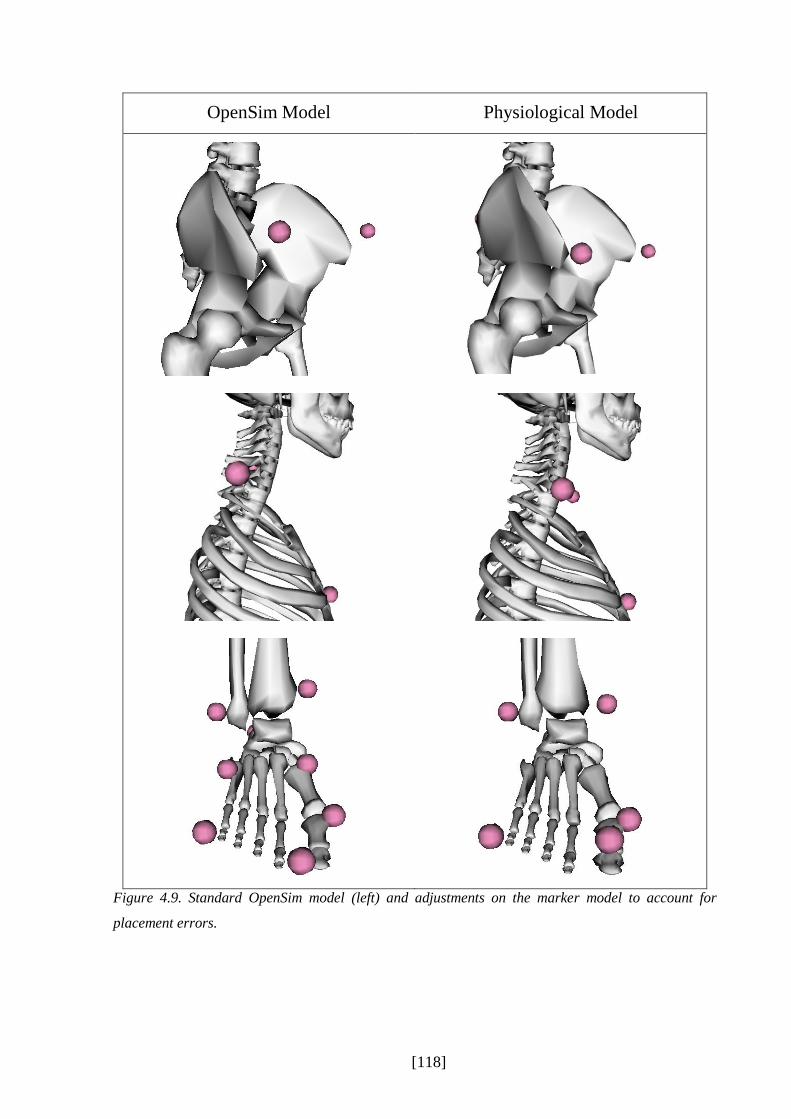
[118]

OpenSim Model Physiological Model

Figure 4.9. Standard OpenSim model (left) and adjustments on the marker model to account for

placement errors.

[119]

The recommendation of OpenSim to subjectively interfere by “preview static pose” is not

applicable in a clinical gait analysis routine as individual decisions may have an influence on

the estimation’s outcome. Therefore, another approach has been developed for scaling the

model. Markers which were chosen to scale the segments of the model were changed and, if

needed, virtually reconstructed. This was done according to the principle of axis alignment: the

line between the scaling markers should be as parallel to the axis to which the segment should

be scaled to (Baker, 2011) to decrease errors in the scaling of the segments. This also means

that, for a better scaling, the segments were not anymore scaled isometric, but separately and

independently in the x,y, and z directions using different marker pairs and, therefore, scaling

factors.

To enhance the scaling according to the principle of axis alignment it was decided to use

experimental marker locations to estimate the position of joint centres and bony anatomical

landmarks which lie directly on the bone in such a way that scaling and fitting can be performed

simultaneously in a manner that is consistent with the biomechanical model. The anatomical

landmarks are estimated on the basis of the measured experimentally calibration marker

positions, the known dimensions of the markers and an estimate of the soft tissue thickness.

Thus, for example, the lateral femoral epicondyle landmark is estimated to be offset by the

marker radius, the thickness of the base plate and the estimated soft tissue artefact from the

measured centre of the marker in the direction of the measured centre of the medial epicondyle

marker. Joint centres are then estimated in relation to these landmarks, for example the knee

joint (in standing) is the mid-point of the medial and lateral epicondyle markers.

During the experimental data collection and processing, marker locations are reconstructed

within Nexus (Nexus 1.8.5, Vicon, T40S cameras). The estimated anatomical landmarks and

joint centres for static trail data are calculated using a customised BodyLanguage model (Vicon,

Oxford, UK) running within Nexus (see appendix A4). In OpenSim, the same bony landmarks

and joint centres were defined as additionally virtual markers in the model for the static trial.

This was done by estimating the locations of the key anatomical landmarks within their

respective coordinate systems from the bony meshes and of the joint centres from the model.

Only these estimated anatomical landmarks and joint centres were then used for the scaling and

fitting of the model (Table 4.1). A weighting of 3:1 in favour of the joint centres biased the

fitting of the principal axes to the joint centres leaving the landmark information to determine

the rotation of segments about those axes. A more detailed description of the adapted scaling

can be found in appendix A5.

[120]

This process includes an additional step into the standardised pipeline. However, it is structured

in such a way that the interacting elements of scaling, fitting and model marker alignment are

automatically satisfied without the requirement for any interaction from the operator. The

calculation of additional anatomical landmarks and joint centres can be easily implemented in

the experimental routine processing of capturing and processing experimental data. Therefore,

for the following experimental study this step will be included into the routine processing and

into the standardised pipeline.

[121]

Table 4.1. Anatomical landmarks and joint centres which are additional included for the static scaling

of the model.

Landmark Derivation

Anterior superior iliac

spine (ASIS)

Marker radius1 and ASIS soft tissue thickness (STT) behind ASIS marker

centre in a direction parallel to the line between the mid-point of the ASIS

markers and the sacral marker.

Sacrum Marker radius and PSIS STT in front of marker centre in a direction parallel

to the line between the mid-point of the ASIS markers and the sacral marker.

Lateral epicondyle Marker radius and knee STT from the marker centre in the direction of the

medial epicondyle marker.

Medial epicondyle Marker radius and knee STT from the marker centre in the direction of the

lateral epicondyle marker.

Lateral malleolus Marker radius and knee STT from the marker centre in the direction of the

medial malleolus marker.

Medial malleolus Marker radius and knee STT from the marker centre in the direction of the

lateral malleolus marker.

Posterior calcaneus Marker radius and heel STT from the marker centre in the direction of the

hallux marker.

Ankle floor Projection of ankle joint centre onto floor.

Posterior calcaneus floor Projection of posterior calcaneus marker onto floor (to ensure plantar surface

of foot is positioned flat on the floor).

Hallux floor Projection of hallux marker centre onto floor.

1st metatarsal phalangeal

joint floor

Projection of 1first metatarsal phalangeal joint marker centre onto floor.

5th metatarsal phalangeal

joint floor

Projection of fifth metatarsal phalangeal joint marker centre onto floor.

Joint Centre

Hip joint centre Scaled in the sagittal plane to the distance between mid-point of ASIS

landmarks and mid-point of PSIS landmarks and in medio-lateral direction to

distance between the ASIS landmarks.

Lumbar sacral joint

centre

Scaled in the sagittal plane to the distance between mid-point of ASIS

landmarks and mid-point of PSIS landmarks.

Knee joint centre Mid-point of lateral and medial epicondyle landmarks.

Ankle joint centre Mid-point of lateral and medial malleolus landmarks.

Mid-acromion point Mid-point of acromion markers.

Note. STT=soft tissue thickness, ASIS=anterior superior iliac spine, PSIS=posterior superior iliac

spince.

[122]

4.4.2 Step 2: Inverse Kinematics in SimTrack

In movement science there exists two different ways of calculating joint angles, either through

direct kinematics or inverse kinematics. Direct kinematics is frequently used in gait analysis

(e.g., PlugInGait) where marker trajectories are measured through time and an algorithm is

applied to calculate the positions of the segments and the kinematics of the joints. Inverse

kinematics uses an optimisation approach to adjust the joint angles in order to fit the trajectory

of virtual markers defined within the model to experimental marker trajectories (Kainz,

Modenese, Carty, & Lloyd, 2014). OpenSim uses the second method in its SimTrack pipeline.

The inverse kinematics tool positions the model in every time frame into a pose which best

matches the experimental marker data by minimising a sum of weight squared marker errors

(equation 5). Additionally, experimental joint coordinates (which can be joint angles) can be

included into this calculation, too, which, however, has not been done for the present study, as

only the experimental marker trajectories were used as the kinematic input. OpenSim

recommends maximum marker errors to be less than 2-4cm, the RMS under 2cm.

Like the static scaling, markers can be weighted which specifies how strongly the error of a

marker should be minimised. The least squares equation which is solved by the inverse

kinematics pipeline is

(5)

where q is the vector of the generalised coordinates (i.e., joint angles), xiexp is the vector of the

position of the experimental marker i and xi(q) is the vector of the position of the corresponding

virtual marker on the model output depending on the generalised coordinates of the model q

(Hicks & Dembia, 2012). The constant wi describes the weightings of the markers. These

weights are defined in the participant’s inverse kinematics setup file and can be changed

manually through the operator. In the standard approach, the pelvis markers as well as the heel

and tip toe markers are rated with 10, whereas all other markers are rated with 1, except the

acromion markers (weight of 0.5) and the head marker (weight of 0.1). Further setting

definitions in the .xml setup file are the time range of the gait cycle, the participant’s adapted

model, and the experimental marker trajectory file.

[123]

The output file of inverse kinematics is a .mot file where following coordinates over the gait

cycle are defined: pelvis tilt, pelvis list, pelvis rotation, hip flexion, hip adduction, hip rotation,

knee flexion, and ankle dorsiflexion. Furthermore, subtalar and MTP angle are defined, too;

however, as both joints are locked for this study they are set to zero. Pelvis tilt describes how

much the pelvis is tilted forward or backward in relation to the sagittal plane, pelvis list

describes the angle of the pelvis in frontal plane.

Adjustments to the SimTrack Inverse Kinematics Tool

The only adjustment to the standard approach is a different weighting of the tracking markers

for the least squared error calculation. With the settings in the standard approach, the marker

errors were too high regarding the guidelines of OpenSim (chapter 5.3.2). Also, the rationale

behind the OpenSim standard weighting of the markers has not been explained in the user

guides or anywhere else. Except the markers on the pelvis (RASIS, LASIS, VSacral) and the

heel markers which were weighted 10 times higher than all other markers, no other marker was

favoured in its weighting. Shank and thigh markers or any other foot marker were not defined

for a higher rating, which, therefore, might lead to bigger tracking errors in the kinematics of

the knee.

This standard weighting has no clinical or anatomical rational for walking purposes,

whatsoever. Tracking markers are important for defining the orientation of the coordinate

reference frame and the position of the segment in space during the movement. Therefore,

markers were weighted as defined in Table 4.2. A weighting of 1 or 2 was chosen, to keep the

weighting throughout tracking markers more homogeneous but also to be able to set the focus

on markers important to define the segments of the lower limb. With this standardised approach

the Inverse Kinematics tool resulted in smaller marker errors (chapter). Besides this change, the

pipeline inverse kinematics is kept on standard settings.

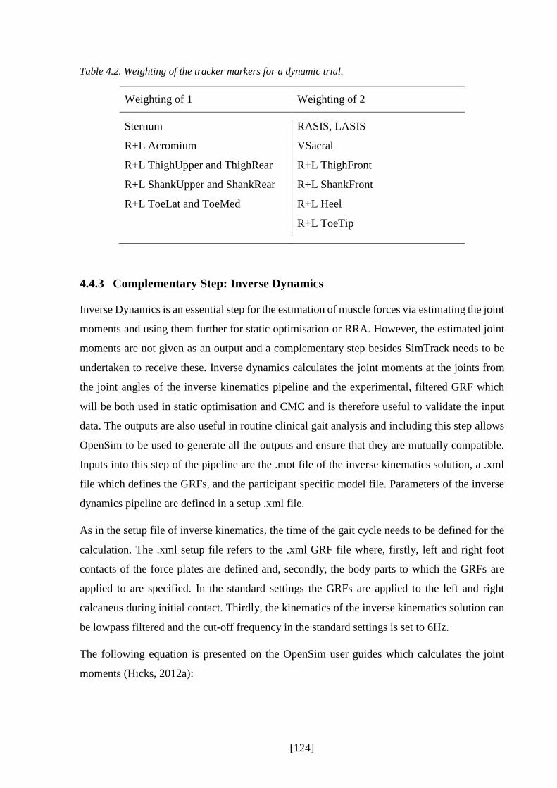
[124]

Table 4.2. Weighting of the tracker markers for a dynamic trial.

Weighting of 1 Weighting of 2

Sternum RASIS, LASIS

R+L Acromium VSacral

R+L ThighUpper and ThighRear R+L ThighFront

R+L ShankUpper and ShankRear R+L ShankFront

R+L ToeLat and ToeMed R+L Heel

R+L ToeTip

4.4.3 Complementary Step: Inverse Dynamics

Inverse Dynamics is an essential step for the estimation of muscle forces via estimating the joint

moments and using them further for static optimisation or RRA. However, the estimated joint

moments are not given as an output and a complementary step besides SimTrack needs to be

undertaken to receive these. Inverse dynamics calculates the joint moments at the joints from

the joint angles of the inverse kinematics pipeline and the experimental, filtered GRF which

will be both used in static optimisation and CMC and is therefore useful to validate the input

data. The outputs are also useful in routine clinical gait analysis and including this step allows

OpenSim to be used to generate all the outputs and ensure that they are mutually compatible.

Inputs into this step of the pipeline are the .mot file of the inverse kinematics solution, a .xml

file which defines the GRFs, and the participant specific model file. Parameters of the inverse

dynamics pipeline are defined in a setup .xml file.

As in the setup file of inverse kinematics, the time of the gait cycle needs to be defined for the

calculation. The .xml setup file refers to the .xml GRF file where, firstly, left and right foot

contacts of the force plates are defined and, secondly, the body parts to which the GRFs are

applied to are specified. In the standard settings the GRFs are applied to the left and right

calcaneus during initial contact. Thirdly, the kinematics of the inverse kinematics solution can

be lowpass filtered and the cut-off frequency in the standard settings is set to 6Hz.

The following equation is presented on the OpenSim user guides which calculates the joint

moments (Hicks, 2012a):

[125]

𝜏 = 𝑀(𝑞)�̈� + 𝐶(𝑞, �̇�) + 𝐺(𝑞) (6)

where q,�̇�, and �̈� are the vectors of generalised positions, velocities and accelerations, M(q) is

the system matrix, C(q,�̇�) is the vector representing the Coriolis and centrifugal forces, G(q)

are the gravitational vector forces, and τ is the vector of the generalised forces on the joints. No

adjustments compared to the standard approach were made for the following experimental

study.

4.4.4 Step 3a: Static Optimisation in SimTrack

The first mathematical model which has been chosen to estimate muscle activations and forces

in the following experimental study is static optimisation. It is an inverse dynamics approach

that attributes the net joint moments to moments arising from a number of individual muscle

forces at each independent instant in time (Hicks & Dembia, 2014). Inputs into the calculations

are the generalised coordinates from the inverse kinematics pipeline (i.e., joint angles) and the

experimental and filtered GRF.

Static optimisation is divided up in two main steps, firstly, the calculation of joint moments

which includes the equation of motions and the experimental input, and secondly, the estimation

of muscle activation and forces via using the characteristics of the musculoskeletal model as

well as a cost function to minimise estimation errors. Therefore, the static optimisation tool

needs the participant’s adjusted .osim model which is the output of the scaling tool, the time

specification of the walking trial, the results of the Inverse Kinematics Tool, the GRFs, and the

specification about the low pass cut-off filter for the kinematic data. In the static optimisation

setup .xml file it can be specified if the muscle force-length curve is included while running the

static optimisation tool, which is set to ‘true’ in the standard approach. The standard objective

function which is used to optimise the muscle force estimation is the overall sum of muscle

activations squared. The exponent of the optimisation criterion can be changed if needed,

however, for the following experimental study the settings were kept on following optimisation

criteria:

∑(𝑎𝑚)2

𝑛

𝑚=1

(7)

[126]

where n is the number of muscles of the model and am the activation level of the muscle m at a

discrete time step. The ideal force generators constrained by the force-length-velocity

properties of m muscle are defined with following formula:

𝜏𝑗 = ∑[𝑎𝑚𝑓(𝐹𝑚0 , 𝑙𝑚, 𝑣𝑚)]𝑟𝑚,𝑗

𝑛

𝑚=1

(8)

where 𝐹𝑚0 is the maximum isometric force, 𝑙𝑚 the length, and 𝑣𝑚 the shortening velocity of the

muscle. 𝑟𝑚,𝑗 defines the moment arm about the jth joint axis and 𝜏𝑗 is the generalised force which

acts about the jth joint axis. As static optimisation is a time independent solution and does not

takes the activation-contraction dynamics into account, the force-length-velocity complex

𝑓(𝐹𝑚0 , 𝑙𝑚, 𝑣𝑚) does not take the contributions from the parallel elastic element into account and

assumes the tendon to be inextensible (Hicks & Dembia, 2014).

For the following experimental study, the static optimisation tool was applied without any

changes to the standard approach. The cut-off frequency of 6Hz for the kinematic input data as

well as the exponent of 2 for the optimisation criterion were kept the same. The static

optimisation tool outputs the estimated muscle activations which define the amount of the

activation of the muscles between a scale of 0 and 1 and the estimated muscles forces.

4.4.5 Step 3b: Residual Reduction Algorithm in SimTrack

The second mathematical model which has been chosen for the estimation of muscle forces is

the method computed muscle control (CMC). However, to be able to use this technique a

preliminary step is required to minimise discrepancies between the dynamics of the system

based on the kinematic analysis and the experimental GRFs. This is called residual reduction

algorithm (RRA). Dynamic inconsistencies are removed by applying nonphysical

compensatory forces and moments known as residuals, while this process also modifies the

kinematics to minimise the size of these (Thelen & Anderson, 2006).

After locking the subtalar and MTP joints, the model has 19 degree of freedoms, each

characterised by a generalised coordinate and actuated by a single actuator. Most of the

coordinates represent joint angles with the actuators representing the action of the muscles

around the relevant axis. Six of the model’s degree of freedom, however, represent the

translation and rotations of the pelvis relative to the ground in all three planes and are actuated

[127]

by actuators representing the nonphysical compensatory forces and moments. These are the

residual actuators providing the residual forces Fx (anterior-posterior), Fy (proximal-distal), and

Fz (medial-lateral), and the residual moments Mx (sagittal), My (frontal), and Mz (transverse)

(Hicks & Uchida, 2013b).

These six residual actuators account for the errors occurring through the experimental data

collection (e.g., noises) and modelling assumptions (e.g., HAT segment) and, therefore, for the

dynamic inconsistency, by adding a new force to the equations. This force balances Newton’s

second law by changing

𝐹 = 𝑚 ∗ 𝑎

to

𝐹 + 𝐹𝑟𝑒𝑠𝑖𝑑𝑢𝑎𝑙 = 𝑚 ∗ 𝑎

(9)

𝐹𝑟𝑒𝑠𝑖𝑑𝑢𝑎𝑙 represents the overall force by the six actuators on the six degrees of freedom on the

pelvis to the ground. The lower these values the less the dynamic inconsistency.

After running the RRA pipeline, the average value for each of the residual actuators is computed

(Fx, Fy, Fz, Mx, My, Mz), and averaged. Mx and Mz are then used to adjust the torso’s centre

of mass to account for an excessive ‘leaning’ of the model (Hicks & Uchida, 2013b) which can

occur by inaccuracies in the segment’s mass distribution or the geometry of the segment.

Furthermore, the RRA outputs recommendations for segments’ mass adjustments of all

segments of the model. This is done by using the averaged value of Fy and dividing it

proportionally up among the model’s segments. It is worth noting that the model’s segments

masses are not adjusted automatically and are only output as a recommendation to the user.

Unfortunately, OpenSim does not provide a pipeline which would include this step into a

routine processing. However, a manual adjustment for every participant and every trial would

be time costly in a clinical gait analysis. As these segment adjustments are highly recommended

in OpenSim a MATLAB script has been used which automatically adjusts the mass of the

segments in the .osim file.

A last step of RRA is to rerun the tracking algorithm that was used to calculate the residuals

based on the original kinematics of the dynamic walking trial. This time the model with adjusted

masses and centres is used and the cost function is modified so that the motion defined

throughout the desired kinematics is generated purely by the internal joint moments.

[128]

4.4.6 Step 3c: Computed Muscle Control in SimTrack

The RRA pipeline outputs the adjusted joint kinematics which are then used for the estimation

of muscle forces in the CMC pipeline. CMC tries to track these set of desired kinematics by

computing a set of muscle excitations that will drive the generalised kinematics of the

musculoskeletal model towards the experimental kinematics (Figure 4.10) (Hicks & Uchida,

2013a). For each time step t CMC loops the process forward to the next time step t+T.

Therefore, the process is a pseudo-forward-dynamics process as not the whole time instant but

only the time steps before and after a specific time step are dependent on each other.

Figure 4.10. Schematic presentation of the CMC pipeline, adapted from Thelen and Anderson (2006).

�⃗⃗� 𝒆𝒙𝒑, �⃗⃗� ̇𝒆𝒙𝒑, �⃗⃗� ̈𝒆𝒙𝒑 are positions, velocities, and accelerations of experimental kinematics, respectively,

�⃗� 𝒈𝒓𝒇𝒆𝒙𝒑

is the GRF vector, kv and kp are feedback gains which weight the current velocity and position

errors �⃗� ̇𝒒 and �⃗� 𝒒 to compute a set of desired accelerations �⃗⃗� ̈𝒅𝒆𝒔. �⃗⃗� are the muscle excitations, whereas

�⃗⃗� and �⃗⃗� ̇ are the generalised coordinates and speeds of the model which are driven towards the

experimental ones.

The first step in CMC is to compute initial states for the model to be able to create initial values

for the muscle states like the muscle activation levels and the muscle fibre length. CMC is

therefore applied to the first 0.03 seconds. However, these 0.03 seconds should be prior to the

desired movement time as during that period the forces can change dramatically until they are

balanced for the actual walking trial (Hicks & Uchida, 2013a). This also allows generalised

coordinates and speeds (joint angles and joint angular velocities) to be computed for the initial

states of the walking trial.

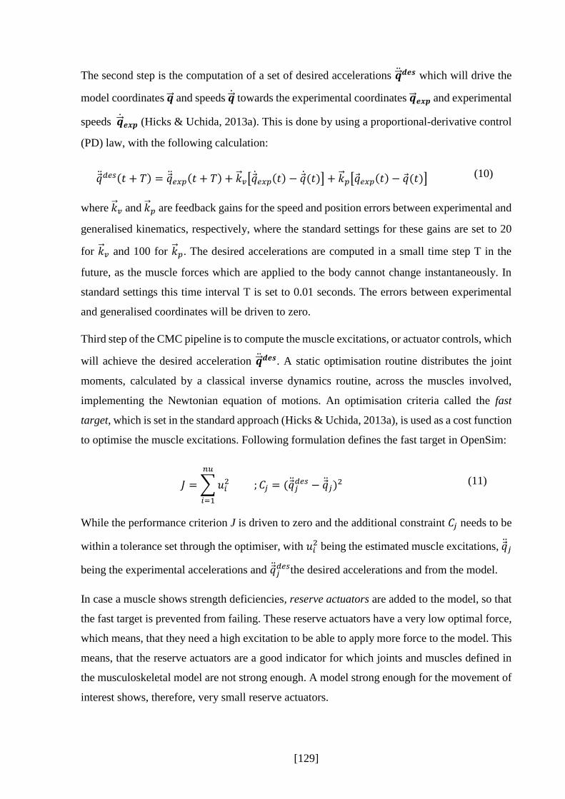
[129]

The second step is the computation of a set of desired accelerations �⃗⃗� ̈𝒅𝒆𝒔 which will drive the

model coordinates �⃗⃗� and speeds �⃗⃗� ̇ towards the experimental coordinates �⃗⃗� 𝒆𝒙𝒑 and experimental

speeds �⃗⃗� ̇𝒆𝒙𝒑 (Hicks & Uchida, 2013a). This is done by using a proportional-derivative control

(PD) law, with the following calculation:

𝑞 ̈𝑑𝑒𝑠(𝑡 + 𝑇) = 𝑞 ̈𝑒𝑥𝑝(𝑡 + 𝑇) + �⃗� 𝑣[𝑞 ̇𝑒𝑥𝑝(𝑡) − 𝑞 ̇(𝑡)] + �⃗� 𝑝[𝑞 𝑒𝑥𝑝(𝑡) − 𝑞 (𝑡)] (10)

where �⃗� 𝑣 and �⃗� 𝑝 are feedback gains for the speed and position errors between experimental and

generalised kinematics, respectively, where the standard settings for these gains are set to 20

for �⃗� 𝑣 and 100 for �⃗� 𝑝. The desired accelerations are computed in a small time step T in the

future, as the muscle forces which are applied to the body cannot change instantaneously. In

standard settings this time interval T is set to 0.01 seconds. The errors between experimental

and generalised coordinates will be driven to zero.

Third step of the CMC pipeline is to compute the muscle excitations, or actuator controls, which

will achieve the desired acceleration �⃗⃗� ̈𝒅𝒆𝒔. A static optimisation routine distributes the joint

moments, calculated by a classical inverse dynamics routine, across the muscles involved,

implementing the Newtonian equation of motions. An optimisation criteria called the fast

target, which is set in the standard approach (Hicks & Uchida, 2013a), is used as a cost function

to optimise the muscle excitations. Following formulation defines the fast target in OpenSim:

𝐽 = ∑𝑢𝑖2

𝑛𝑢

𝑖=1

; 𝐶𝑗 = (𝑞 ̈𝑗𝑑𝑒𝑠 − 𝑞 ̈𝑗)

2 (11)

While the performance criterion J is driven to zero and the additional constraint 𝐶𝑗 needs to be

within a tolerance set through the optimiser, with 𝑢𝑖2 being the estimated muscle excitations, 𝑞 ̈𝑗

being the experimental accelerations and 𝑞 ̈𝑗𝑑𝑒𝑠the desired accelerations and from the model.

In case a muscle shows strength deficiencies, reserve actuators are added to the model, so that

the fast target is prevented from failing. These reserve actuators have a very low optimal force,

which means, that they need a high excitation to be able to apply more force to the model. This

means, that the reserve actuators are a good indicator for which joints and muscles defined in

the musculoskeletal model are not strong enough. A model strong enough for the movement of

interest shows, therefore, very small reserve actuators.

[130]

The last step of CMC is a forward dynamics solution advancing forward in time T to compute

the generalised kinematics of time t+T by using the computed muscles excitations u while

considering the equations of motion. Furthermore, with the knowledge of the muscular-tendon

characteristics of the musculoskeletal model, muscle activations and forces are estimated for

the time step t+T. The three steps consisting of computing the desired accelerations, the static

optimisation routine, and the forward dynamics simulation are driving the CMC forward in T

time steps until the end of the walking trial is reached. The upper and lower bounds for muscle

excitations are set to 1 (maximum excitation) and 0.02 (minimum excitation) in the standard

settings. They cannot reach zero because, as defined in the OpenSim user guides (Hicks &

Uchida, 2013a), musculoskeletal models do often not behave according to the physiological

pattern if they are able to switch the excitation totally off.

Adjustments to the SimTrack Computed Muscle Control Tool

Most of the standard settings in CMC are kept the same. However, one main change has been

undertaken which, in the end, enhanced the muscle force estimation output. The standard time

steps of CMC are set to 0.01 seconds. With this setting, especially in swing, the estimated

muscle excitations and forces were unstable (Figure 4.11). However, with changing the time

steps from 0.01 to the half of 0.005 seconds, the muscle forces were much smoother. Figure

4.11 shows estimated muscle forces of five normal walking trials throughout a gait cycle of one

typical participant for a standard 0.01 seconds time step CMC calculation and with changed

time steps to 0.005 seconds. Reason for this smoothening from 0.01 to 0.005 seconds might be

the shorter time frame in which CMC can adjust the muscle excitations to the new acceleration

conditions of the segments. This process is time-independent, i.e. each time step is handled

independently in relation to the adjacent time frames, which might initiate a greater change with

bigger time frames. However, an adjustment in dividing the time steps in half means a double

as long estimation time for CMC. The 0.005 seconds have been chosen after balancing accuracy

and time efficiency and discussing this issue with several OpenSim researchers as well as

researchers who applied OpenSim during walking and experienced the same problem.

[131]

Figure 4.11. Estimated tibialis anterior muscle forces with CMC for five normal walking trials of a

typical participant while keeping the standard settings by 0.01 seconds per time step (above) and

changing the time steps to 0.005 seconds (below).

4.4.7 Final Structure of the OpenSim Pipeline for the Experimental Study

This Chapter could improve the standard pipeline SimTrack of OpenSim while adjusting it to

a more physiological and clinical approach which is needed for the purpose of this study.

Especially the scaling approach is novel compared to OpenSim’s standard settings, as the model

can be scaled individually along the axes of the system and not isometric in all three directions.

Table 4.3 summarises adjustments which have been undertaken in the different steps of

OpenSim’s SimTrack to estimate muscle forces during healthy walking. Summarised, some

adjustments were undertaken to make the standard SimTrack more applicable for the clinical

gait analysis. Firstly, the markers on the musculoskeletal model were adjusted according to the

placement in the clinic and a more physiological definition (e.g., the ASIS marker), secondly,

additional joint centres and anatomical landmarks were calculated to be able to scale the

segments closer to the principle of axis alignment, thirdly, segments were scaled non-isometric

[132]

and independently in all three directions, fourthly, the marker weighting for the static inverse

kinematics pipeline were changed according to the calibration markers, fifthly, the subtalar and

the MTP angle were locked due to high errors with CMC, sixthly, the marker weighting for the

dynamic trial were adapted, too, seventhly, the experimental GRFs were filtered before to input

into any of the pipelines, and eighthly, the calculation time steps of CMC was changed from

0.01 to 0.005 seconds per time step.

These adjustments were all tested beforehand by small pilot studies; however, the whole

adjusted OpenSim pipeline to estimate muscle forces needs to be tested now for a larger

population. This will be presented in the next chapter (chapter V), where ten healthy participants

were tested in a VICON motion system while walking at five different speeds to be able to

systematically control the results of the estimation while changing the known influencing

parameter speed. The muscle force estimations will be compared to parallel captured surface

EMG of some of the muscles of the lower limb for validation. Furthermore, static optimisation

and computed muscle control are analysed and compared to each other to possible find the best

estimation technique for the clinical gait analysis routine.

Table 4.3. Summarised adaptations which have been undertaken on the standard SimTrack pipeline for

the implementation into a routine clinical gait analysis.

Steps Changes to the standard SimTrack pipeline

1 - Additional calculation of joint centres and anatomical landmarks

- Adapted marker weighting and adapted segment scaling

2 - Adapted marker weighting

3a No changes

3b No changes

3c - Changed calculation time steps (0.005)

[133]

CHAPTER V

5 Experimental Implication of a Standardised Protocol to

Estimate Muscle Forces for Routine Clinical Gait

Analysis

5.1 Introduction

OpenSim and its implemented musculoskeletal model from Delp and colleagues (1990)

represents an attractive modelling and simulation tool to be applied into clinical gait analysis.

The operator has access to the source code of the musculoskeletal model and this allows the

operator to adjust this model to suit the purposes of the study (see chapter IV). With the

adjustments undertaken in chapter IV on the provided pipeline SimTrack in OpenSim the

operator does not need to interfere with any step of the process anymore. All virtual markers

have been placed on the correct anatomical landmarks within the musculoskeletal model. The

developed enhanced scaling approach enables a systematic and physiological scaling of the

model.

This chapter will test this developed standardised pipeline by implementing it into a classical

gait analysis routine. This will facilitate an analysis of the robustness of the pipeline while

controlling some of the factors which influence the estimation of muscle activations and forces.

Currently, no gold standard relating to muscle force estimation is available; thus other ways of

validating estimated muscle forces are needed. In their recent work Hicks and colleagues (2015)

point out the importance of validating the estimations output to independent experiments or

other models. They suggest EMG data as a validation tool to determine if the muscle

coordination of the estimated muscle forces correlates to the experimental captured EMG

activity.

Important, however, is a validation tool independent to the estimation process (Hicks et al.,

2015). As chapter III showed, most studies using EMG as a validation tool also incorporated

EMG data into their estimation process to define the neural input (Bogey et al., 2005) or applied

constraints to prevent what are perceived as non-physiological activations (Collins, 1995). To

[134]

date, the literature lacks a detailed validation of estimated muscle activations and forces with

independent EMG measurements. A key focus of this research is to assess the match of non-

EMG constrained; OpenSim derived activation and force estimations with independent EMG

data. Surface EMG will be simultaneously captured during the experimental data acquisition of

kinematics and kinetics, on the same participants and trials. This will minimise inter- and intra-

variability between participants and trials while keeping EMG independent from the estimation

process.

Walking speed is one of the main factors influencing experimental outputs. Differences in

walking speed result in changes in joint angles, ground reaction forces (Lelas et al., 2003) and

EMG (Schwartz et al., 2008). The change in joint kinematics can lead to differences in the

contractile state (fibre length, velocity) of each muscle and, therefore, lead to differences in the

generation of muscle forces (R.R. Neptune et al., 2008). This information is important,

especially in a clinical gait analysis routine when comparing a patient group with the healthy

population. Differences caused by factors such as walking speed need to be known to exclude

them from other changes initiated by the impairment of the patient. Therefore, this experimental

study will systematically control the walking speed to analyse speed-dependent changes on

muscle force estimation.

One of the studies using EMG excitations as a comparison tool in relation with speed

dependence is the study of Neptune and colleagues (R.R. Neptune et al., 2008). Nonetheless,

they used these experimental EMG excitations within their estimation process to define the

muscle excitation patterns, causing a bias of their validation technique. Also, they only

presented the EMG speed changes for the soleus and medial gastrocnemius. Additionally, the

estimated muscle force of the gastrocnemius has been defined by summating the medial and

lateral modelling compartments together, whereas only the EMG excitations of the medial

gastrocnemius were used for comparison. Their data show the changes caused by different

walking speeds averaged across all participants, but individual muscle force estimations

compared with individual EMG excitations were not presented. This may underestimate

individual differences as well as inter-subject variability due to missing standard deviation

bands. Lastly, it is also not clear how many trials for each participant were included into the

estimation and graphical representation.

Another study has been undertaken by Liu and colleagues (M. Q. Liu, Anderson, Schwartz, &

Delp, 2008) who used OpenSim to provide reference data about muscle contributions to the

support and progression of locomotion across different walking speeds of eight children

[135]

(12.9±3.3 years). The musculoskeletal model gait2392 was used in a computed muscle control

(CMC) estimation. Again, differences in muscle forces caused by different walking speeds were

detected. However, the number of experimental trials included is unclear and cited as “at least

one double-stance phase on the force plates at each walking speed”. Only muscle force data of

children were provided, kinematic and kinetic input data were extracted from the data pool of

Schwartz and colleagues (2008). The graphs show averaged curves of the estimated muscle

forces with underlined EMG standard deviation bands. These EMG signals, however, show

only the average excitation of all eight participants, but do not include individual comparison

of muscle estimations and EMG excitations. The study also merely used EMG excitation data

for the whole quadriceps and the plantarflexors and not for single muscles.

In summary, the literature is lacking comprehensive analyses of muscle force estimations on

both healthy and pathological adults and, additionally, the dependence of walking speeds

compared to individual EMG excitations. The first stage of implementing such standardised

measurement protocol into the clinic is to provide and validate normative reference data.

Therefore, this study will estimate muscle forces of the lower limb in a healthy adult population

while walking at different speeds using the developed standardised protocol (chapter IV). Static

optimisation and CMC which are both most suitable for the clinical daily routine (chapter III)

will be both tested and applied in OpenSim. Both approaches will be validated against

individual surface EMG measurements and compared in reference to the shape and speed-

dependent changes.

The pipeline SimTrack additionally provides joint angles through the Inverse Kinematics Tool

and joint moments through the complementary tool Inverse Dynamics. To be able to implement

the whole pipeline clinically it would be useful to know the compatibility of OpenSim’s joint

angles and moments compared to current clinical models like the Conventional Gait Model.

Therefore, as a subsidiary step, joint angles and moments are additionally calculated in Vicon

Nexus with the use of the PlugInGait model to analyse the usefulness of OpenSim as a whole

package for the implementation onto the routine clinical gait analysis.

The results of the study will provide information about the robustness of the developed

standardised protocol and about the potential to implement this protocol into the clinical gait

analysis. This study aims to provide a base for a normative data pool for subsequent clinical

trials. Furthermore, it will distinguish between the two estimation methods to define the model

most suitable for a clinical use.

[136]

5.2 Methods

This chapter will define the methods used to conduct the experimental study to implement the

developed protocol to estimate muscle forces. Participants’ characteristics and experimental

data collection as well as the processing of experimental and estimated data are explained.

Detailed information about the OpenSim modelling process can be found in chapter IV. Ethical

approval for the experimental study was granted by the College of Health and Social Care

Ethics Panel (appendix A6).

5.2.1 Participants

Ten healthy adults, five male and five female, were recruited from the University of Salford

student and employee population and participated in this study. The population group has been

restricted to healthy adults to avoid influences caused by different age groups or disabilities

(Winter et al., 1990). Participants received an information sheet beforehand (appendix A7) and

filled out a research consent form (appendix A8) after being introduced to the purpose, the

procedure and potential risk of the study. It was clearly indicated to the participants that they

are able to interrupt or stop the participation at any time without explanation.

5.2.2 Laboratory Set-up and Calibration

The study has been undertaken in the movement laboratory of the University of Salford. The

laboratory is equipped with a Vicon motion analysis system including ten infra-red cameras

(Vicon 1.8.5, 100Hz, T40S cameras) and four force plates mounted into the walkway to capture

the ground reaction forces (Kistler, 1000Hz, 2x 9286A, 2x 9253A) (Figure 5.1). The origin of

the global reference frame was set on one of the corners of the first force plate. The surface

EMG excitations were collected in parallel with a wireless 16 channel Noraxon system using

an in-built low pass filter of 500Hz (DTS receiver, 1000Hz). Data from the following muscles

were collected on both legs: rectus femoris, vastus medials and lateralis, semitendinosus, tibialis

anterior, soleus, gastrocnemius medialis and lateralis (Table 5.1).

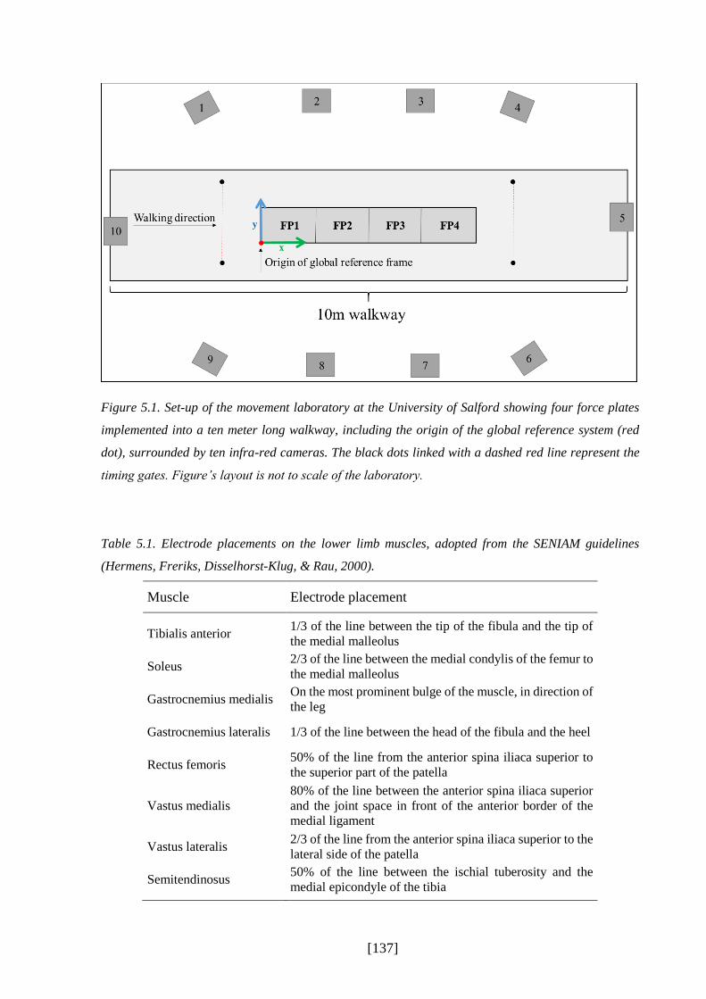
[137]

Figure 5.1. Set-up of the movement laboratory at the University of Salford showing four force plates

implemented into a ten meter long walkway, including the origin of the global reference system (red

dot), surrounded by ten infra-red cameras. The black dots linked with a dashed red line represent the

timing gates. Figure’s layout is not to scale of the laboratory.

Table 5.1. Electrode placements on the lower limb muscles, adopted from the SENIAM guidelines

(Hermens, Freriks, Disselhorst-Klug, & Rau, 2000).

Muscle Electrode placement

Tibialis anterior 1/3 of the line between the tip of the fibula and the tip of

the medial malleolus

Soleus 2/3 of the line between the medial condylis of the femur to

the medial malleolus

Gastrocnemius medialis On the most prominent bulge of the muscle, in direction of

the leg

Gastrocnemius lateralis 1/3 of the line between the head of the fibula and the heel

Rectus femoris 50% of the line from the anterior spina iliaca superior to

the superior part of the patella

Vastus medialis 80% of the line between the anterior spina iliaca superior

and the joint space in front of the anterior border of the

medial ligament

Vastus lateralis 2/3 of the line from the anterior spina iliaca superior to the

lateral side of the patella

Semitendinosus 50% of the line between the ischial tuberosity and the

medial epicondyle of the tibia

[138]

Before starting the measurement, the capture volume was calibrated with a calibration wand so

that the infra-red cameras were calibrated according to the origin of the global measurement

volume and the position of the force plates. Furthermore, the force plates’ centre of pressure

(CoP) and the direction of the GRF vector of each force plate were tested using the so-called

CalTester method (Figure 5.2) (Goldberg, Kepple, & Stanhope, 2009), where a metal plate was

temporarily placed on top of each force plate and fixed with double sided tape. This plate was

provided with a small notch where a metal rod equipped with five reflecting markers could be

inserted. This ensured that the CoP on the force plate and the tip of the metal rod stayed

consistent throughout the testing and prevent that a moment is created. One trial per force plate

was captured while the metal rod was placed onto the notch. The rod was then moved in circles

around the notch while keeping pressure on the metal rod. To ensure that during the trial the

force was consistently passing through the rod, a metal bar could be placed on top of the rod so

that the operator was able to apply a consistent force. The orientation of the tip position of the

rod and the CoP could then be calculated by the force platform data and be compared with the

orientation and position of the notch delivered by the motion system.

Figure 5.2. Principle of the CalTester. A rod is placed onto a small notch provided on a metal plate

(black square) which is temporarily placed on the force plate (grey square) and fixed with double sided

tape. Another metal bar can be placed on top of the rod, again provided with a small notch, to ensure

that the force vector is passing through the rod. Five markers are placed alongside the rod. The arrows

define where the operator should place pressure on the rod while moving the rod in circles.

[139]

5.2.3 Participant Preparation

To place the electrodes onto the skin the SENIAM (Surface Electromyography for the Non-

Invasive Assessment of Muscles) guidelines were applied (Hermens & Freriks; Merletti &

Hermens, 2000). After gently shaving the skin to ensure a minimisation of artefacts resulting

out of small hairs between the skin and the electrodes, the skin was prepared with an abrasive

paste. This insures a lower impedance between electrode and skin and a good fixation of the

electrodes, which also reduces the risk of artefacts (Hermens et al., 2000). The skin was then

gently cleaned with disinfectant pads before the electrodes were placed along the muscle fibres

as defined by the SENIAM guidelines. The reflective marker set which has been described in

detail in chapter IV was placed. Additional markers were placed on the right and left posterior

iliac spine and on top of the tarso-metatarsal joint to allow parallel use of the Conventional Gait

Model which is used in Vicon (PlugInGait) (Baker, 2013). The same experimenter positioned

the reflective markers as well as the wireless EMG sensors, which were fixed with double sided

tape and placed on the required positions and landmarks. To minimise skin movement artefacts

the markers were placed on bony landmarks or on a part of the segment with less skin

movement.

5.2.4 Data Collection

After taking required anthropometric data from the participant (height, mass, knee and ankle

width) the participant was asked to stand stationary on one of the force plates while the operator

captured a static trial. This enables the musculoskeletal model in OpenSim to be scaled as well

as the joint centre locations in Vicon to be calculated relative to the local coordinate systems of

the segments (Davis III et al., 1991). The participant stood still with the arms gently crossed in

front of the chest so that all markers were visible with the shoulders still in a neutral position.

This trial was also used to measure the body mass of the participant for the OpenSim pipeline.

After the representative static trial had been captured, the participant walked at his/her self-

selected speed straight over the force plates on a ten meter walkway. The participant was asked

to continue walking until five gait cycles each starting with the right and left foot were recorded.

All trials required that both feet during the foot contact phase were fully placed on top of one

of the force plates so that the whole GRF related to the body mass could be captured. To be

sure that the participants walked in their most normal walking pattern, targeting was not

allowed. Although some studies have shown that variations to spatiotemporal patterns (Verniba,

[140]

Vergara, & Gage, 2015) and ground reaction forces (Grabiner, Feuerbach, Lundin, & Davis,

1995) may not be significant, it is generally assumed that visual targeting of the force plates

should be avoided due to the risk of an unnatural walking pattern (Oggero, Pagnacco, Morr,

Simon, & Berme, 1998; Perry & Burnfield, 2010).

This procedure was repeated for 20% and 40% slower and faster walking speeds. This was

monitored with timing gates placed five meters apart the start and end of the force plates

alongside the plane of progression. Participants were given feedback on their speed to guide

them to walk at the prescribed speed to within 1%. The faster walking trials were set to the end

of the testing session to prevent the participant of an early stage of fatigue. Therefore, the

walking protocol was arranged in following order with the inclusion of at least five right and

five left valid walking trials each: 1. Self-selected walking speed, 2. 20% slower, 3. 40% slower,

4. 20% faster, 5. 40% faster.

The EMG excitations were recorded with Vicon Nexus and synchronised with the motion

capture system. However, a time delay of 312ms of the wireless EMG system needed to be

taken into account resulting from the wireless settings of the system. Before the actual start of

the measurement and after placing the EMG electrodes a cross-talk check of all the EMG

muscle excitations was undertaken by asking the participant to activate separately the muscles

of interest. During the measurement session some of the trials were pre-processed to ensure the

quality of the EMG excitations. Also, during the measurement the force plates were regularly

reset to zero to receive accurate ground reaction force data.

5.2.5 Data processing

After the data collection procedure, the raw marker trajectories were pre-processed in Vicon by

a customised pipeline to calculate a number of virtual landmarks and joint centres (see chapter

IV.4.1 for more details) and then, including the raw ground reaction force data, exported in an

ASCII file for further processing. The ground reaction forces were filtered in MATLAB

(2012b) with a 6Hz low-pass 2nd order Butterworth filter and automatically replaced in the

ASCII file. All these files were then imported into an OpenSim tool called Lee-Son’s Toolbox

(S. Lee & Son, 2010). This tool re-formats the data to be compatible with OpenSim. Raw

marker trajectory data in Vicon for the Conventional Gait Model (which is used for comparison)

were filtered with a Woltering routine including a mean standard error of 10.

[141]

The surface EMG signals were separately exported out of Vicon into .c3d files and further

processed in MATLAB (2012b) by using an EMG analyser tool which has been developed from

the University of Salford (version 1.3, Phil Tresadern). This tool contains a two stage process

where, firstly, the .c3d files are converted into MATLAB files which, secondly, are further used

to process and filter the EMG excitations. By defining the gait cycle prior in Vicon the trial can

be automatically cut to the time of interest. EMG signals are then high-pass filtered with a 20Hz

Fast Fourier transform filter in addition to the 500Hz low-pass filter of the NORAXON system.

To create a linear envelope of the muscle excitations the signals are finally filtered with a 6Hz

low-pass 2nd order Butterworth filter and then finally exported into an ASCII file.

To be able to compare the surface EMG patterns to the estimations of muscle activations and

forces the magnitude of the signals need to be normalised (Burden, 2010). To date,

normalisation of EMG excitations are highly discussed in the literature, but no gold standard

has been defined yet (Perry & Burnfield, 2010). Pilot work suggests that attempts to normalise

the EMG excitations using maximum voluntary contraction tests on a dynamometer (KinCom)

led to excessive inter-participant variability (in agreement with Clarys, 2000). The results of

the pilot data of this study showed that normalising to the average muscle EMG excitation

across the gait cycle is a more time efficient but still reliable technique. Therefore, the average

excitation value across a typical gait cycle at very fast walking speed has been chosen for

normalisation.

As described in chapter IV of this work, the simulation tool OpenSim has been chosen for this

study to estimate the muscle activations and forces during healthy walking. The adapted

musculoskeletal model gait2392 was implemented using the adjusted pipeline defined in

chapter IV for the estimation process. This includes the scaling of the musculoskeletal model,

the calculation of the joint angles using inverse kinematics, and the calculation of joint moments

using inverse dynamics. Furthermore, both optimisation methods static optimisation and CMC

including the pre-step residual reduction algorithm (RRA) were selected (chapter IV) and used

to estimate muscle activation and forces. For the comparison with surface EMG the estimated

excitations (actuator controls) of CMC were used and not the latter calculated activations as the

CMC excitations are closer to the experimental surface EMG excitations (chapter IV). Static

optimisation provides only the muscle activations which were chosen for comparison with

surface EMG.

[142]

5.2.6 Data Analysis

To analyse the quality of the Scaling Tool the overall mean as well as maximal RMS marker

errors across all ten participants will be stated and discussed and compared to OpenSim’s

recommendations. Also, scaling factors of individual segments are averaged across participants

and presented. Marker fitting errors of the Inverse Kinematics Tool will be averaged and the

overall mean and maximal RMS errors across all ten participants will be presented.

Furthermore, estimated joint angles with OpenSim will be descriptively compared to joint

angles which were calculated with the standard Conventional Gait Model (PlugInGait) in Vicon

while taking the average for self-selected walking speed. The same comparison will be

undertaken with estimated joint moments.

RMS values for the Scaling Tool and the Inverse Kinematics Tool were calculated as follows:

firstly, a RMS value for each participant was calculated separately by taking the RMS value for

each gait cycle which then is averaged to gain a mean RMS value for that participant; secondly,

the overall mean and maximal RMS value are calculated across all ten participants by using the

calculated individual mean RMS values of each participant.

The body mass adjustment within RRA is presented for each participant and walking speed

separately, whereas the torso’s centre of mass adjustment is averaged across participants and

its distribution presented across walking speeds. Additionally, adjusted joint angles with RRA

are compared to results of the Inverse Kinematics Tool. Averaged ground reaction force and

moment residuals of RRA and CMC’s reserve actuators of the hip, knee and ankle moments

across participants are presented for each walking speed and compared to the recommendations

of OpenSim.

The activation/excitations and forces which have been estimated with static optimisation and

CMC are presented and descriptively analysed for the tibialis anterior, gastrocnemius medialis

and lateralis, soleus, semitendinosus, rectus femoris, and vastus medialis and lateralis.

Estimated muscle activation/excitation are compared to surface EMG for each walking speed

averaged across corresponding walking trials to validate estimations in shape and speed-

dependence. Estimated muscle forces are compared to corresponding activation/excitations of

static optimisation/CMC. Additionally, results of three participants are exemplarily presented

to demonstrate individual differences.

[143]

5.3 Results

The measurement duration for a testing session took in average approximately two and a half

hours. Participants walked at a self-selected walking speed of 1.28±0.12m/s which lies within

the values in the literature (Bohannon & Williams Andrews, 2011). Participants’ characteristics

are displayed in Table 5.2.

Table 5.2. Participants’ characteristics, including age, gender, height in meter, and mass in kilograms.

Participant Age Gender Height (m) Mass (kg)

P01 29 F 1.62 55.80

P02 24 M 1.81 95.21

P03 41 M 1.73 65.00

P04 27 M 1.83 74.31

P05 23 F 1.69 70.95

P06 28 M 1.69 61.88

P07 29 F 1.63 65.75

P08 30 F 1.68 57.80

P09 26 M 1.84 72.99

P10 27 F 1.72 61.57

Average 28.40 5M:5F 1.72 68.13

SD 4.95 0.08 11.35

The following results were achieved for the calibration of the measurement system: the standard

wand calibration of the Vicon system resulted in an average camera image error of

0.103±0.007mm, whereas the results of the caltester revealed an average force orientation error

of 1.9±1.5° and an displacement vector between the centre of pressure (CoP) location estimated

by the force plate and the endpoint of the caltester of -1.99±2.41mm in direction of progression

(x-axis), 8.03±5.74mm in the vertical direction (y-axis), and -0.32±0.91mm in the lateral-

medial direction (z-axis).

For two participants, one EMG sensor was not functioning throughout the measurement session

through an unexplained error. It was decided to not interrupt and stop the session but to go on

as planned taking the not functioning EMG sensor into account.

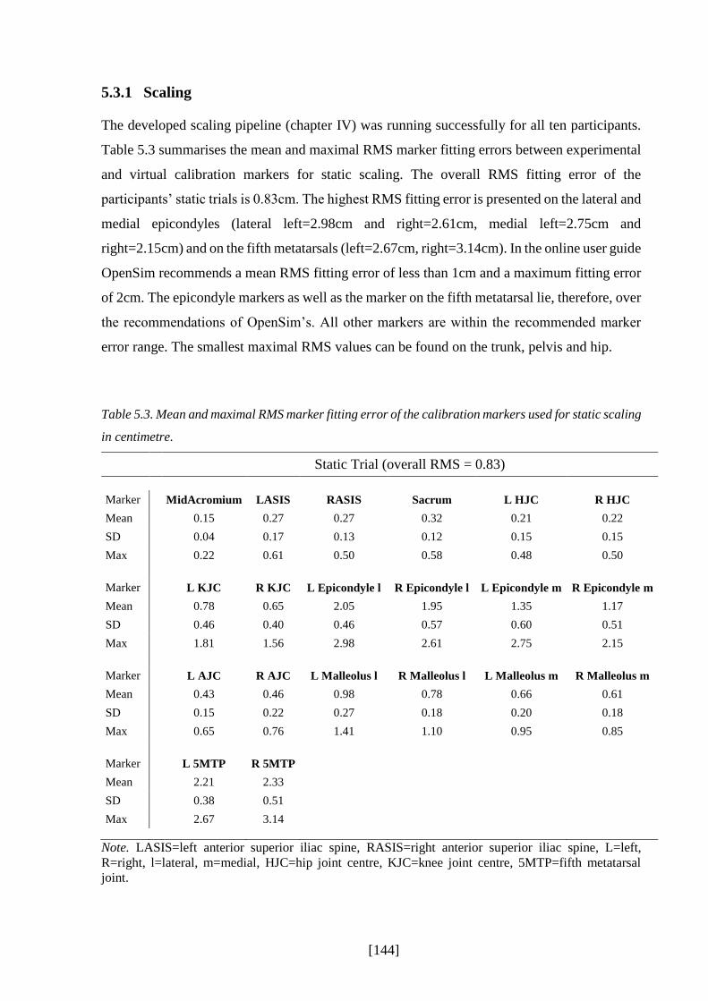
[144]

5.3.1 Scaling

The developed scaling pipeline (chapter IV) was running successfully for all ten participants.

Table 5.3 summarises the mean and maximal RMS marker fitting errors between experimental

and virtual calibration markers for static scaling. The overall RMS fitting error of the

participants’ static trials is 0.83cm. The highest RMS fitting error is presented on the lateral and

medial epicondyles (lateral left=2.98cm and right=2.61cm, medial left=2.75cm and

right=2.15cm) and on the fifth metatarsals (left=2.67cm, right=3.14cm). In the online user guide

OpenSim recommends a mean RMS fitting error of less than 1cm and a maximum fitting error

of 2cm. The epicondyle markers as well as the marker on the fifth metatarsal lie, therefore, over

the recommendations of OpenSim’s. All other markers are within the recommended marker

error range. The smallest maximal RMS values can be found on the trunk, pelvis and hip.

Table 5.3. Mean and maximal RMS marker fitting error of the calibration markers used for static scaling

in centimetre.

Static Trial (overall RMS = 0.83)

Marker MidAcromium LASIS RASIS Sacrum L HJC R HJC

Mean 0.15 0.27 0.27 0.32 0.21 0.22

SD 0.04 0.17 0.13 0.12 0.15 0.15

Max 0.22 0.61 0.50 0.58 0.48 0.50

Marker L KJC R KJC L Epicondyle l R Epicondyle l L Epicondyle m R Epicondyle m

Mean 0.78 0.65 2.05 1.95 1.35 1.17

SD 0.46 0.40 0.46 0.57 0.60 0.51

Max 1.81 1.56 2.98 2.61 2.75 2.15

Marker L AJC R AJC L Malleolus l R Malleolus l L Malleolus m R Malleolus m

Mean 0.43 0.46 0.98 0.78 0.66 0.61

SD 0.15 0.22 0.27 0.18 0.20 0.18

Max 0.65 0.76 1.41 1.10 0.95 0.85

Marker L 5MTP R 5MTP

Mean 2.21 2.33

SD 0.38 0.51

Max 2.67 3.14

Note. LASIS=left anterior superior iliac spine, RASIS=right anterior superior iliac spine, L=left,

R=right, l=lateral, m=medial, HJC=hip joint centre, KJC=knee joint centre, 5MTP=fifth metatarsal

joint.

[145]

Bony segments of the generic musculoskeletal model were scaled independently in its principle

axis (proximal-distal P-D) compared to both other axis (anterior-posterior A-P, medial-lateral

M-L). Scaling factors differ slightly between segments as well as between different dimensions

(Figure 5.3). The biggest discrepancy was within the femur, with the transverse plane scaling

factors about 40% larger than those for the primary axis and showing most variability as well

(as represented by standard deviation bars). By contrast, the tibia was scaled about 20% less in

the transverse plane than along its primary axis. All other scaling factors were similar.

Figure 5.3. Mean and one standard deviation bars representing the scaling factors of the bony segments

of the generic musculoskeletal model gait2392 in all three directions anterior-posterior (A-P), medial-

lateral (M-L), and proximal-distal (P-D). Blue indicates the primary axis, green both other axes.

[146]

5.3.2 Inverse Kinematics

The results of the least square error problem which has been solved during inverse kinematics

are listed in Table 5.4. This table includes one typical self-selected walking trial per participant

and presents the tracking markers. The overall mean RMS error reached 0.91cm which lies

within the recommended OpenSim user guidelines for dynamic fitting (<2cm). None of the

markers exceeded the recommended mean RMS value; the highest mean fitting error is shown

on the thigh markers and on the tip toe marker. It is further recommended that the maximum

fitting errors should not exceed 4cm. This only occurs on the right medial toe marker with an

error of 6.82cm.

Table 5.4. Mean and maximal RMS marker fitting error in centimetre of the tracking markers used for

one typical walking trial during inverse kinematics.

Dynamic Trial (overall RMS = 0.91)

Marker LAcromium RAcromium Sternum LASIS RASIS VSacral

Mean 0. 82 0.75 0.85 0.86 0.81 0.65

SD 0.32 0.24 0.44 0.23 0.22 0.21

Max 2.36 2.17 2.29 2.33 2.32 1.89

Marker RThighFront RThighUpper RThighRear RShankFront RShankUpper RShankRear

Mean 1.07 1.14 1.00 0.76 0.87 0.79

SD 0.20 0.22 0.20 0.12 0.19 0.16

Max 2.69 2.75 3.25 3.94 3.50 3.42

Marker LThighFront LThighUpper LThighRear LShankFront LShankUpper LShankRear

Mean 1.14 1.18 1.02 0.82 0.88 0.75

SD 0.16 0.29 0.26 0.20 0.40 0.35

Max 2.61 2.93 2.32 2.14 2.79 2.61

Marker LHeel RHeel LToeTip RToeTip LToeLat RToeLat

Mean 0.85 0.82 1.12 1.14 1.01 0.98

SD 0.18 0.16 0.26 0.17 0.16 0.16

Max 2.97 3.39 3.71 3.83 3.55 3.00

Marker LToeMed RToeMed

Mean 0.76 0.83

SD 0.21 0.21

Max 1.89 6.82

Note. L=left, R=right, LASIS=left anterior superior iliac spine, RASIS=right anterior superior iliac

spine, lat=lateral, med=medial.

[147]

In general, estimated joint angles are comparable with results in the literature (for example

Perry & Burnfield, 2010). In this study, the experimental data have also been fully processed

using the Conventional Gait Model PlugInGait in Vicon to compare them with the results in

OpenSim. A typical comparison of the joint angles of participant P02 can be found in Figure

5.4. The patterns for both the joint angles of the OpenSim solution and the PlugInGait solution

are overall similar to each other. However, some differences are detected. Firstly, the pelvis tilt

and hip flexion are slightly higher for the results of PlugInGait than for OpenSim. Secondly,

the hip abduction’s pattern in swing phase is different between the two approaches. Thirdly,

both the knee flexion peak values are higher with the OpenSim approach than with PlugInGait.

And, fourthly, the ankle dorsiflexion for the results received with PlugInGait shows, especially

in swing, a higher plantar flexion. Furthermore, the dorsiflexion in OpenSim is earlier and

increased in swing.

[148]

Figure 5.4. Mean and one standard deviation of joint angles calculated in OpenSim (red) and Vicon

Nexus (blue) for five right walking trials of one typical participant (P02) during self-selected walking

speed.

Averaged joint angles estimated with OpenSim for all ten participants at their self-selected

walking speed including both the right and left gait cycle are shown in Figure 5.5. In general,

there exists a low variability between participants; however, a high standard deviation band is

shown around the mean for pelvic tilt and, therefore, a higher variability than in the other planes

Blue= Vicon

Red = OpenSim

[149]

of the pelvis (pelvis list, pelvis rotation). Additionally, knee flexion in stance phase shows an

increased standard deviation at the first peak. This variability, however, has also been shown

previously in the literature (Kadaba et al., 1989; Winter, 1990).

Figure 5.5. Average joint angles of OpenSim across five right and five left walking trials of all ten

participants during self-selected walking speed.

[150]

5.3.3 Joint Moments

Estimated joint moments are not used as an input in the muscle force estimation pipeline but

are a good indicator of the quality of kinematic and kinetic modelling. They, however, are

frequently discussed in clinical gait analysis and thus are of interest in their own right. Figure

5.6 shows the internal joint moments of the hip, knee and ankle during self-selected walking

speeds for one typical participant calculated with OpenSim and compared with the results from

Vicon.

Figure 5.6. Mean and one standard deviation internal joint moments (Nm) calculated in OpenSim (red)

and Vicon (blue) for five trials each of one typical participant during normal walking.

Like the findings for the joint kinematics, an overall agreement between the results of

PlugInGait and OpenSim is shown. However, some small differences can be detected as well:

the hip flexion moment has more prominent peaks for the PlugInGait solution than for the

Blue= Vicon

Red = OpenSim

[151]

results of OpenSim; however, for the frontal and transverse plane it is the other way round.

Also, the magnitude as well as the standard deviation band of the hip rotation moment is smaller

with PlugInGait than with OpenSim. The magnitude during mid stance of the knee flexion

moment is higher with OpenSim than with Vicon. Compared to the hip and knee joint moments,

the ankle plantar flexion moment is consistent between Vicon and OpenSim.

Figure 5.7 presents the average internal joint moments including the right and left gait cycle for

all ten participants for self-selected walking speeds. The consistency between participants is

again high; increased standard deviation bands can be found at peak joint moments and at the

ankle during 20 to 30% of the gait cycle.

Figure 5.7. Average internal joint moments of OpenSim (Nm) for ten participants including five right

and left gait cycles for self-selected walking speeds.

[152]

5.3.4 Muscle Activations/Excitations and Force Estimations

The results of estimated muscle activations of static optimisation and the excitations of CMC

are compared to surface EMG. The estimation’s pattern as well as speed-dependent changes

will be evaluated and individual results of three participants additionally presented in his

section. Furthermore, estimated muscle forces will be compared to corresponding

activations/excitations including speed-dependent and participant specific evaluations of the

results.

The computational time which was needed to successfully run muscle force estimation for one

trial were about one minute for static optimisation and 30 minutes for CMC. Before presenting

the muscle activations and forces the results of CMC’s pre-step RRA will be presented.

5.3.4.1 Results of the Residual Reduction Algorithm

In general, the residual reduction algorithm ran successfully. However, for some of the walking

trials RRA crashed during processing. This affected walking trials from six out of the ten

participants (P02-P04, P06, P09, P10). Fast (8 trials) and very fast (13 trials) walking trials

failed most commonly. Additionally, the left very fast walking trials of participant P06 and the

right fast walking trials of P09 were crashing throughout with RRA. Apart from the faster

walking speeds, only one trial for slow and one for very slow walking failed (P03). The

OpenSim output file which is given after every step of the OpenSim pipeline defines the failure

of RRA as follows:

CMC.computeControls: ERROR- Optimizer could not find a solution.

Unable to find a feasible solution at time = 2.857.

Model cannot generate the forces necessary to achieve the target acceleration.

Possible issues: 1. not all model degrees-of-freedom are actuated,

2. there are tracking tasks for locked coordinates, and/or

3. there are unnecessary control constraints on reserve/residual actuators.

Table 5.5 presents the body mass adjustments, relatively distributed across all segments, which

were carried out by the RRA Tool to adjust the kinematics to be more consistent with the

experimental ground reaction forces (chapter IV). The biggest change in participants’ body

mass is shown for the very fast walking trials, where the average mass adjustment is -

1.69±1.10kg with the smallest and greatest individual mass adjustment of -0.29kg and -3.31kg,

[153]

respectively. The body mass during very fast walking speeds have, therefore, been all corrected

in negative direction, resulting in a smaller body mass than before. However, for the other

walking speeds some of the participants’ body masses have been adjusted slightly upwards

towards a greater body mass, with 0.67kg for participant P04 while walking at self-selected

walking speed.

Table 5.5. Overall adjusted mass (kg) through RRA for all ten participants divided up in five walking

speeds, averaged across all ten trials.

Participant Walking speed

Very slow Slow Self-selected Fast Very fast

P01 0.01 0.07 0.16 0.40 -0.29

P02 -1.59 -1.39 -0.23 -0.60 -1.42

P03 -1.60 -1.41 -0.48 -1.24 -3.31

P04 -0.11 0.18 0.67 -0.25 -0.94

P05 -1.27 -1.05 -1.35 -1.88 -2.61

P06 0.32 0.50 0.57 0.57 -2.10

P07 0.12 -0.04 -0.20 -0.16 -3.25

P08 -0.32 -0.23 -0.32 -0.10 -0.34

P09 -0.25 -0.30 0.12 -0.65 -1.56

P10 -0.17 -0.17 -0.10 0.00 -1.09

Average Mean -0.49 -0.38 -0.12 -0.39 -1.69 SD (0.72) (0.67) (0.57) (0.74) (1.10)

The walking speed with the smallest averaged mass adjustment is the self-selected walking

speed with -0.12±0.57kg. During this speed all participants show a mass adjustment under

±0.5kg, except two participants who are slightly over (0.57kg, 0.67kg) and one participant who

is clearly over ±0.5kg (-1.35kg). However, the latter represents a participant with a general

mass adjustment of 1kg or more throughout all walking trials.

Another parameter which is adjusted while running RRA is the torso’s centre of mass (CoM)

in medial-lateral as well as anterior-posterior direction which leads into a better consistency

between kinematics and experimental GRFs. Average adjustments across all ten participants

can be found in Figure 5.8. The torso CoM is moved anterior closer to the sternum compared

to its original position across all walking speeds. However, from very fast (1.64cm) to very

slow walking (3.88cm) a slight increase in the amount of adjustments in anterior-posterior

direction can be detected. Here, the standard deviations stays similar across speeds. Different

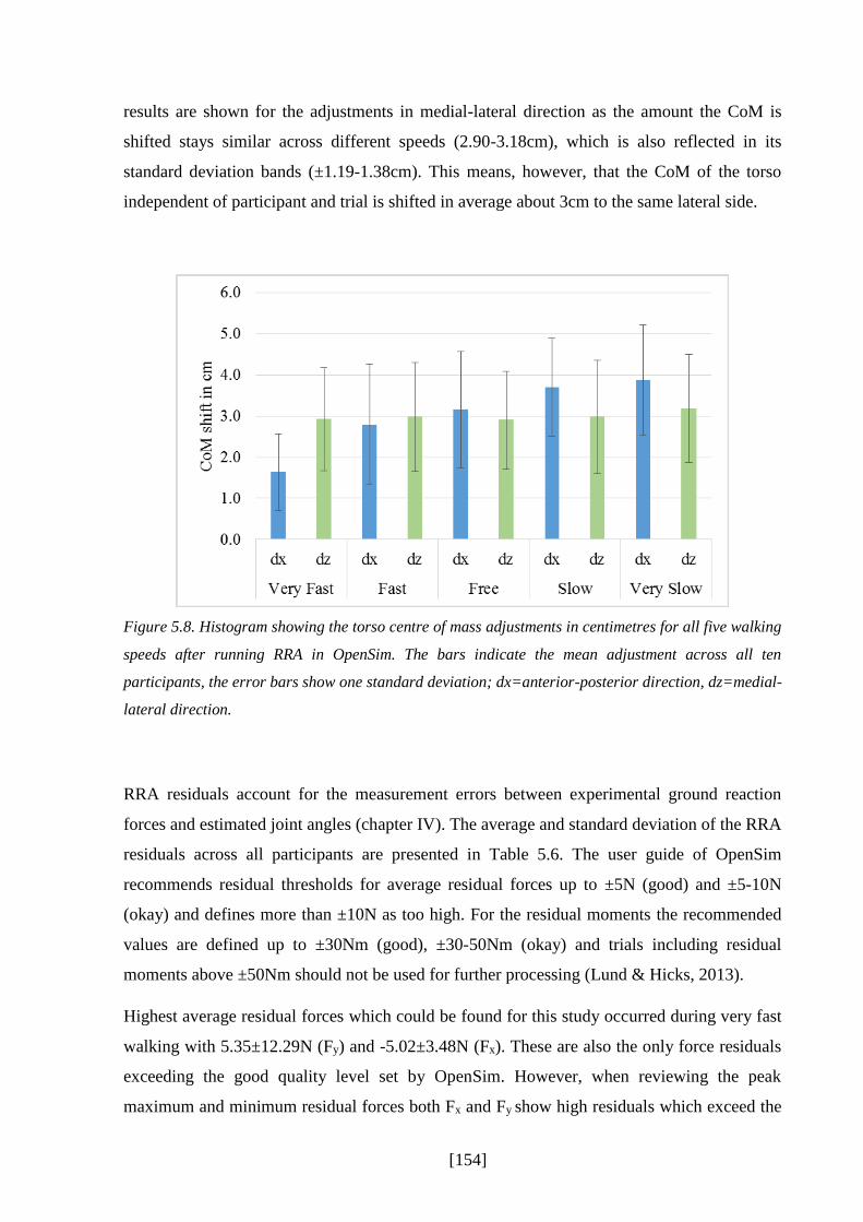
[154]

results are shown for the adjustments in medial-lateral direction as the amount the CoM is

shifted stays similar across different speeds (2.90-3.18cm), which is also reflected in its

standard deviation bands (±1.19-1.38cm). This means, however, that the CoM of the torso

independent of participant and trial is shifted in average about 3cm to the same lateral side.

Figure 5.8. Histogram showing the torso centre of mass adjustments in centimetres for all five walking

speeds after running RRA in OpenSim. The bars indicate the mean adjustment across all ten

participants, the error bars show one standard deviation; dx=anterior-posterior direction, dz=medial-

lateral direction.

RRA residuals account for the measurement errors between experimental ground reaction

forces and estimated joint angles (chapter IV). The average and standard deviation of the RRA

residuals across all participants are presented in Table 5.6. The user guide of OpenSim

recommends residual thresholds for average residual forces up to ±5N (good) and ±5-10N

(okay) and defines more than ±10N as too high. For the residual moments the recommended

values are defined up to ±30Nm (good), ±30-50Nm (okay) and trials including residual

moments above ±50Nm should not be used for further processing (Lund & Hicks, 2013).

Highest average residual forces which could be found for this study occurred during very fast

walking with 5.35±12.29N (Fy) and -5.02±3.48N (Fx). These are also the only force residuals

exceeding the good quality level set by OpenSim. However, when reviewing the peak

maximum and minimum residual forces both Fx and Fy show high residuals which exceed the

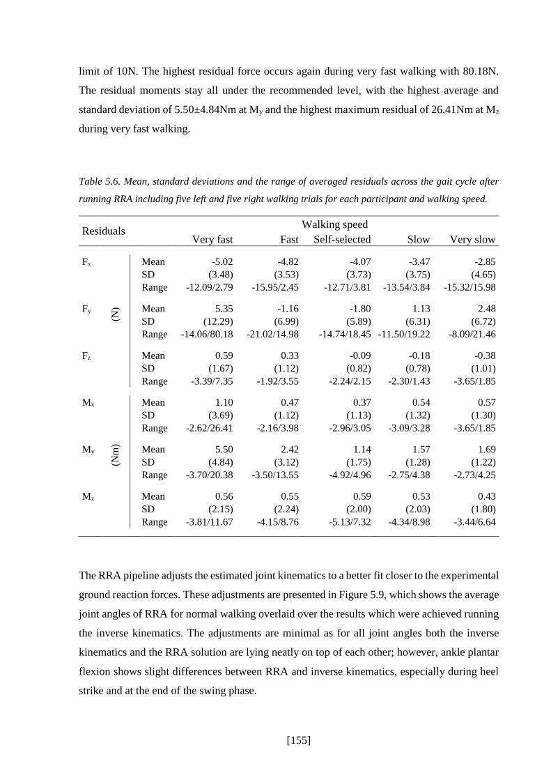
[155]

limit of 10N. The highest residual force occurs again during very fast walking with 80.18N.

The residual moments stay all under the recommended level, with the highest average and

standard deviation of 5.50±4.84Nm at My and the highest maximum residual of 26.41Nm at Mz

during very fast walking.

Table 5.6. Mean, standard deviations and the range of averaged residuals across the gait cycle after

running RRA including five left and five right walking trials for each participant and walking speed.

Residuals Walking speed

Very fast Fast Self-selected Slow Very slow

Fx

(N)

Mean -5.02 -4.82 -4.07 -3.47 -2.85 SD (3.48) (3.53) (3.73) (3.75) (4.65)

Range -12.09/2.79 -15.95/2.45 -12.71/3.81 -13.54/3.84 -15.32/15.98

Fy Mean 5.35 -1.16 -1.80 1.13 2.48 SD (12.29) (6.99) (5.89) (6.31) (6.72) Range -14.06/80.18 -21.02/14.98 -14.74/18.45 -11.50/19.22 -8.09/21.46

Fz Mean 0.59 0.33 -0.09 -0.18 -0.38 SD (1.67) (1.12) (0.82) (0.78) (1.01) Range -3.39/7.35 -1.92/3.55 -2.24/2.15 -2.30/1.43 -3.65/1.85

Mx

(Nm

)

Mean 1.10 0.47 0.37 0.54 0.57 SD (3.69) (1.12) (1.13) (1.32) (1.30) Range -2.62/26.41 -2.16/3.98 -2.96/3.05 -3.09/3.28 -3.65/1.85

My Mean 5.50 2.42 1.14 1.57 1.69 SD (4.84) (3.12) (1.75) (1.28) (1.22) Range -3.70/20.38 -3.50/13.55 -4.92/4.96 -2.75/4.38 -2.73/4.25

Mz Mean 0.56 0.55 0.59 0.53 0.43 SD (2.15) (2.24) (2.00) (2.03) (1.80) Range -3.81/11.67 -4.15/8.76 -5.13/7.32 -4.34/8.98 -3.44/6.64

The RRA pipeline adjusts the estimated joint kinematics to a better fit closer to the experimental

ground reaction forces. These adjustments are presented in Figure 5.9, which shows the average

joint angles of RRA for normal walking overlaid over the results which were achieved running

the inverse kinematics. The adjustments are minimal as for all joint angles both the inverse

kinematics and the RRA solution are lying neatly on top of each other; however, ankle plantar

flexion shows slight differences between RRA and inverse kinematics, especially during heel

strike and at the end of the swing phase.

[156]

Figure 5.9. Adjusted kinematics through the pipeline RRA (red) compared to the results of inverse

kinematics (blue) during normal walking, averaged across all 10 participants including both right and

left.

[157]

5.3.4.2 Results of Estimated Muscle Excitations and Activations Compared to EMG

Static optimisation ran successfully for all ten participants. However, like with RRA CMC

crashed for some of the walking trials as well. None of the participants had a success rate of

100% with CMC. The highest failure rate occurred during trials for very fast walking (14 trials

out of overall 100 very fast walking trials), but all walking speeds were affected. Slow and very

slow were, however, the walking speeds with the least failures (three trials each). Normal and

fast walking speeds resulted in nine and six unsuccessful trials, respectively. In case CMC failed

and crashed during the calculation process, the same output message then with RRA was

specified.

As explained in chapter IV, reserve actuators are applied in CMC to make up for possible

strength deficiencies in muscles. Because these reserve moments have, by definition, a very

low optimal force and thus require very high excitations to apply substantial forces they are an

indicator of muscles that are too weak as specified in the musculoskeletal model (Hicks &

Uchida, 2013a). OpenSim recommends average reserves under 10Nm and peak reserves under

25Nm (good) or between 25-50Nm (okay). Average reserves on the hip, knee, and ankle joints

across all ten participants are presented in Table 5.7, including the maximal and minimal reserve

actuator which occurred across all trials. The mean and standard deviation of all joint moment

reserves do not exceed OpenSim’s recommendations. However, in some cases participant

specific maximal and minimal values are greater than 50Nm, especially for the ankle

plantarflexors. Highest peak reserve actuator can be detected at the knee flexors with -147Nm.

With decreasing walking speeds the number of reserve actuators which lie within the

recommendations increases. Furthermore, average reserve values are generally smaller with

slower walking speeds than with faster walking speeds.

[158]

Table 5.7. Average, standard deviations, maximum and minimum reserve actuators of the hip, knee, and

ankle joints for CMC.

Walking Speeds

Very Fast Fast Self-selected Slow Very Slow

Hip

flexion Mean 0.227 0.077 0.016 0.011 0.007

SD 0.263 0.119 0.063 0.026 0.008

MAX 35.952 35.466 28.352 29.675 32.389

MIN -11.457 -7.846 -8.392 -2.020 -2.157

Hip

adduction Mean -0.279 -0.113 -0.036 -0.018 -0.015

SD 0.276 0.110 0.035 0.024 0.010

MAX 7.113 7.407 0.977 0.480 0.033

MIN -34.963 -13.874 -12.192 -8.217 -15.257

Hip

rotation Mean 0.374 0.234 0.102 0.025 0.017

SD 0.426 0.286 0.134 0.064 0.022

MAX 34.707 35.349 32.512 9.198 3.744

MIN -19.701 -6.583 -6.725 -2.501 -4.622

Knee

flexion Mean -0.277 -0.135 -0.068 -0.038 -0.029

SD 0.250 0.152 0.125 0.047 0.030

MAX 59.007 50.298 40.347 38.991 81.657

MIN -94.260 -71.520 -146.766 -105.631 -77.137

Ankle

plantar flexion

Mean 1.305 0.761 0.438 0.251 0.197

SD 0.718 0.395 0.260 0.128 0.084

MAX 127.837 106.229 109.396 88.271 118.406

MIN -41.611 -43.890 -27.733 -29.252 -23.819

Note. SD=standard deviation, MAX=maximum, MIN=minimum.

By using a static optimisation procedure, CMC calculates muscle excitations called actuator

controls which are further processed to estimate muscle forces. However, for this study the

CMC excitations resulted in heavily noisy patterns (Figure 5.10). To be able to compare the

CMC excitations in its shape and speed-dependence with surface EMG, it has been decided that

these estimated excitations were filtered with the same 6Hz low-pass 2nd order Butterworth

filter which has been applied to create a linear envelope over the muscle EMG excitations. To

be consistent while validating estimated data with surface EMG, activations of static

optimisation were also filtered with the same 6Hz low-pass filter.

[159]

Figure 5.10. Example data of estimated muscle excitations with CMC of the tibialis anterior, vastus

medialis and lateralis, non-filtered (above) and filtered with a 6Hz low pass 2nd order Butterworth filter

(below) for walking trials of all speeds (light grey to dark grey=very slow to very fast) for one

participant (P01).

Averaged static optimisation’s muscle activations, CMC’s muscle excitation and surface EMG

excitations including one standard deviation across all ten participants for the self-selected

walking speed are presented in Figure 5.11. Estimated peak values range between less than 0.2

(semitendinosus, vastus medialis) up to 1 (tibialis anterior, soleus). Normalised peak surface

EMG excitations’ range between 2.5 and 4.5 times an average EMG excitation across a typical

walking trial.

The shapes and magnitudes between CMC and static optimisation are similar for all muscles

except for the tibialis anterior. Here, CMC results in relatively high excitation patterns close to

an activation of 1 which occur during the stance-swing transition, whereas static optimisation

stays below an activation of 0.3. Another difference between CMC and static optimisation is

the second peak of vastus medialis and lateralis around 80% of the gait cycle which is nearly

not present for static optimisation but quite dominant for CMC. Small differences can be also

found for the semitendinosus, where a third peak around 60% of the gait cycle occurs with

CMC but is nearly not visible for static optimisation, and for the rectus femoris, where the peak

value is slightly shifted between CMC and static optimisation (75% to 55%). Furthermore, for

some of the muscle excitations of CMC a sharp and high peak is presented for the first

percentage of the gait cycle. However, this may be due to the first 0.03 seconds which are used

for the initial states needed for the CMC pipeline and are prone to be unstable.

The pattern of most estimated muscle excitations/activations are in general agreement with the

surface EMG excitations. However, four main differences could be detected. Firstly, the peak

[160]

close to the stance-swing transition which has been estimated for the semitendinosus has not

been captured with surface EMG as the EMG signal stays silent during this period. Secondly,

rectus femoris estimation during heel strike and at the end of stance is relatively small or totally

absent with the use of CMC and static optimisation compared to surface EMG. On the other

side, between 30-70% of the gait cycle, the muscle estimations peak, whereas surface EMG

shows only a small peak compared to the peak at heel strike and at the end of swing. Thirdly,

the dominant peak for vastus lateralis and medialis at the end of swing is missing when using

static optimisation, and peaks earlier with CMC. And fourthly, estimated results for the

gastrocnemius lateralis and medials show both a second smaller peak at the end of the gait cycle

which is not present with EMG.

The participants’ inter-variability is mostly similar between static optimisation, CMC, and

surface EMG as the standard deviation bands are comparable with each other compared to the

mean. However, CMC excitations of the gastrocnemius medialis have a slight higher standard

deviation for the descending activation after the peak around 40-50% of the gait cycle compared

to static optimisation and surface EMG. Similar results occur for the tibialis anterior, where the

standard deviation band of CMC at the end of swing is higher than with static optimisation or

EMG.

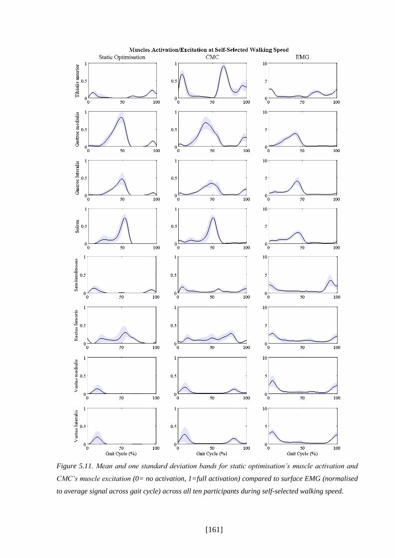
[161]

Figure 5.11. Mean and one standard deviation bands for static optimisation’s muscle activation and

CMC’s muscle excitation (0= no activation, 1=full activation) compared to surface EMG (normalised

to average signal across gait cycle) across all ten participants during self-selected walking speed.

[162]

Figure 5.12 to Figure 5.19 show the averaged muscle excitation of CMC compared to the

activation of static optimisation and to surface EMG across all five walking speeds. Each figure

presents the dependence of walking speed of one single muscle.

Tibialis anterior

Both estimation methods show nearly no speed-dependent influence on the tibialis anterior

(Figure 5.12) which is comparable with the results of EMG. The average activation of static

optimisation and CMC’ excitation stay similar across walking speeds, except a longer activation

after the first peak with slower walking speeds is evident for both mathematical models (10-

50% of the gait cycle). The peak values in swing are slightly increasing with speed but stay

within the range of the standard deviation bands. This difference with speed is not shown for

EMG. Here, the only speed-dependent difference is a small increase of the whole signal during

very fast walking compared to the other walking speeds. Again, however, the change stays

within the standard deviation bands. In general, the standard deviation bands increase from very

slow to very fast for both mathematical models and EMG.

[163]

Figure 5.12. Mean and one standard deviation bands for static optimisation’s muscle activation and

CMC’s muscle excitation of the tibialis anterior compared to surface EMG across five walking speeds

including all ten participants.

[164]

Gastrocnemius medialis and lateralis

Both muscles of the gastrocnemius show in general dependence in speed (Figure 5.13 and Figure

5.14). The maximum peak increases with speed around 45-50% of the gait cycle as well as the

small peak at the end of swing. Gastrocnemius medialis reaches slightly higher estimation

values than lateralis of up to 1 during very fast walking. CMC estimations show additionally a

second smaller peak during descending form the first peak at about 55% of the gait cycle for

very slow and slow walking which is not shown for static optimisation. This is also shown for

gastrocnemius lateralis, however, to a lesser extent. The estimations of CMC show another

small peak after foot contact (5% of the gait cycle) for both gastrocnemius lateralis and medialis

which is not shown for the estimation of static optimisation.

The different patterns of CMC are also not shown for surface EMG, except for very fast

walking, where a small peak occurs during the first 10% of the gait cycle. Another difference

between mathematical models and EMG is the peak at the end of swing which is not present

with EMG. EMG, however, shows similar speed-dependent results than CMC and static

optimisation, although an increased rise between fast and very fast walking is seen which is not

seen to such an extent with both modelling techniques. The standard deviation bands of the

gastrocnemius medialis for all three techniques stay the same throughout walking speeds except

EMG’s very fast walking, whereas gastrocnemius lateralis shows increasing standard deviation

bands with faster walking speeds for both modelling techniques and EMG.

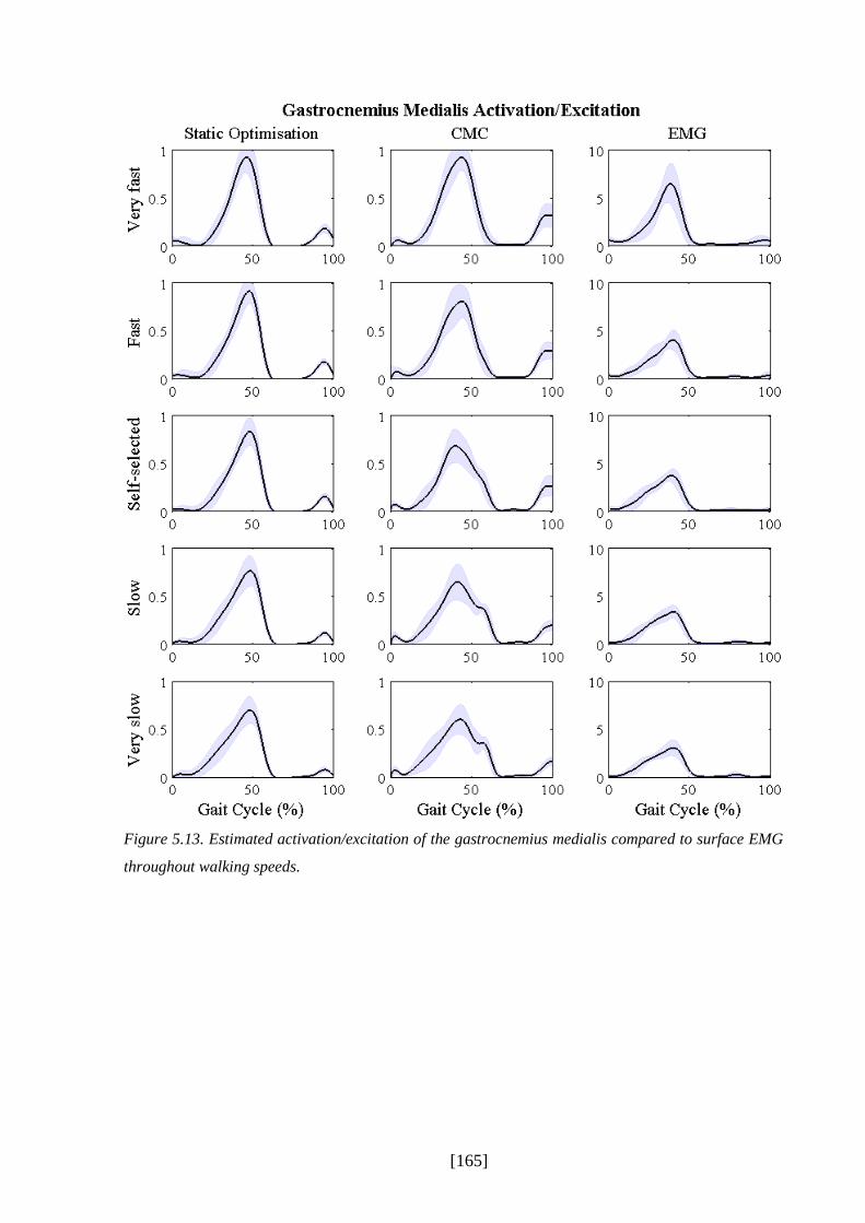
[165]

Figure 5.13. Estimated activation/excitation of the gastrocnemius medialis compared to surface EMG

throughout walking speeds.

[166]

Figure 5.14. Estimated activation/excitation of the gastrocnemius lateralis compared to surface EMG


[167]

Soleus

Like the gastrocnemius, the soleus shows dependence with different walking speeds for static

optimisation and CMC (Figure 5.15). The maximal peak around 50% of the gait cycle increases

and occurs slightly earlier with faster speeds. Static optimisation additionally shows an increase

of the small activation plateau between 20-30% of the gait cycle which develops into a small

peak for fast and very fast walking. This is not shown in such an extent for CMC. EMG shows

as well an increase from very slow to very fast with the same increased rise between fast and

very fast than with the gastrocnemius. The small activation plateau between 0-30% of the gait

cycle rises, too, but does not develop into a peak. The standard deviation bands do not change

greatly between speeds, only EMG shows a great increase for very fast walking.

Semitendinosus

The estimations of the semitendinosus for both static optimisation and CMC are changing with

walking speed (Figure 5.16). Especially the first peak after initial foot contact (about 5-10% of

the gait cycle) rises with increased speed. The second peak at the end of the gait cycle changes

to a lesser extent for static optimisation and stays the same throughout speeds for CMC which

is also true for the third peak of CMC. Only CMC’s estimation during very fast walking shows

a general rise in excitation in stance. Static optimisation develops a third peak with increasing

walking speeds, too, which occurs a bit earlier than for CMC (45% of the gait cycle) and is

shown for fast and very fast walking.

Compared to the mathematical models, EMG shows no great speed-dependence between very

slow and fast walking; only the second peak at the end of swing is increasing with speed.

Contrary to this, EMG’s very fast walking shows a general increase and additionally smaller

peaks between 40-60% of the gait cycle which is accomplished by an increase in the standard

deviation band. In general, the standard deviation band increases with speed for static

optimisation and CMC but stays the same for EMG except very fast walking.

[168]

Figure 5.15. Estimated activation/excitation of the soleus compared to surface EMG throughout walking

speeds.

[169]

Figure 5.16. Estimated activation/excitation of the semitendinosus compared to surface EMG


[170]

Rectus femoris

All three techniques static optimisation, CMC, and EMG increase in their magnitude with speed

(Figure 5.17). However, the shapes of them differ between each other. Static optimisation has

throughout walking speeds a peak at about 55% of the gait cycle which is accomplished by a

small activation plateau between 20-75% of the gait cycle. The peak as well as the plateau to a

lesser extent increase with walking speeds. A small activation at the start of the gait cycle is

present throughout walking speeds but does not change greatly. A second small activation at

the end of the gait cycle is developed for fast and very fast walking. CMC on the other side

presents a small excitation plateau from 10-90% of the gait cycle with a small peak at the end

of swing for very slow walking. With faster walking speeds the plateau increases and develops

first a peak at about 80% of the gait cycle which is then followed by a second higher peak for

fast and very fast walking at about 50% of the gait cycle.

Surface EMG when compared to the modelling techniques shows a different change throughout

walking speeds. The peak at the start and at the end of the gait cycle increasing while the EMG

signal stays low between 20-90% of the gait cycle. This changes with fast and very fast speeds

where a third peak occurs at about 45% of the gait cycle. All three techniques show increased

standard deviation bands with increasing speed.

Vastus medialis and lateralis

Both compartments of the vastus which are included in this study (medialis, lateralis) behave

similarly for both mathematical models and EMG, while vastus lateralis has higher estimations

than medialis (Figure 5.18 and Figure 5.19). In general, a speed-dependence for all three

techniques can be detected. The peak at about 20% of the gait cycle is increasing with walking

speed for static optimisation and CMC. This is also shown for the results of the EMG

measurements with a slightly earlier peak than the modelling techniques. CMC’s second peak

about 80% of the gait cycle increases with speed, too, and occurs slightly earlier with faster

walking speeds. This second peak is not shown for all walking speeds with static optimisation.

EMG develops a third peak about 45% of the gait cycle during very fast walking. Again, EMG’s

very fast walking results have an increased rise in activation to all the other speeds. The standard

deviation bands for static optimisation and CMC increase slightly with walking speeds for both

vastus medialis and lateralis which is also shown for the EMG measurements.

[171]

Figure 5.17. Estimated activation/excitation of the rectus femoris compared to surface EMG throughout

walking speeds.

[172]

Figure 5.18. Estimated activation/excitation of the vastus medialis compared to surface EMG


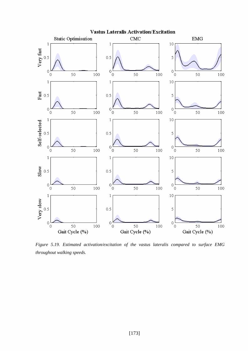
[173]

Figure 5.19. Estimated activation/excitation of the vastus lateralis compared to surface EMG


[174]

The following figures (Figure 5.20 to Figure 5.22) show exemplary individual results of three

participants’ estimated muscle activation (static optimisation) and muscle excitation (CMC)

patterns for all five walking speeds compared to surface EMG. Light blue represents very slow

which increases to dark blue for very fast walking. The three participants which were chosen

differ in their body mass, body height, and gender. P02 (1.81m, 95.21kg) and P04 (1.83m,

74.31kg) are male, whereas P04 is additionally close to the anthropometrics of the generic

model of gait2392 (1.80m, 75.16kg). P08 (1.68m, 57.8kg) is female, and represents one of the

smallest and lightest participants which were included into the study.

Participant P02

Figure 5.20 presents the results of participant P02. In general, the muscle excitations of CMC

and muscle activations of static optimisation show an increase in the magnitude with faster

speeds which is also shown with surface EMG. Some muscles show a nice speed-dependent

pattern change for all three techniques, like for the gastrocnemius medialis, where after initial

contact the force raises later as faster the speed is, but then develops a steeper curve and higher

peak for the fast speeds compared to the slow speeds. Faster speeds can reach an activation

level of 1 for the triceps surae muscles for both static optimisation and CMC. This is also present

for the tibialis anterior of CMC, however, not with static optimisation where the activation stays

under 0.5.

Some of the muscles show a speed-dependent change between very slow and slow walking

speeds with the mathematical model estimations, which is different for EMG where no change

between very slow and slow across all muscles can be seen. Especially fast and very fast

walking speeds experience a great rise in activation for both the modelling techniques and

EMG. The tibialis anterior of the CMC estimation shows two different pattern between the slow

walking speeds compared to self-selected and fast walking speeds at the end of the gait cycle,

where the excitation decreases for slower walking speeds after 90% of the gait cycle and further

rises for the faster walking speeds until the end of the gait cycle. The surface EMG excitation

changes slightly its pattern for some of the muscles for very fast walking. For the muscles on

the thigh additional surface EMG peaks occur which are not present for the other walking

speeds. For example a peak at 40% of the gait cycle occurs for vastus medialis and lateralis,

whereas the muscle is inactive for the rest of the walking speeds. This behaviour is not shown

with the mathematical models.

[175]


activations, CMC’s muscle excitations compared to surface EMG excitations for five different walking

speeds; dark blue=very fast to light blue=very slow.

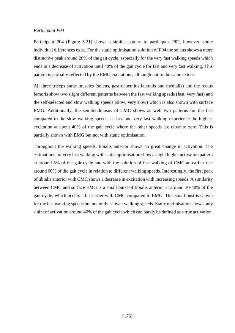
[176]

Participant P04

Participant P04 (Figure 5.21) shows a similar pattern to participant P02, however, some

individual differences exist. For the static optimisation solution of P04 the soleus shows a more

distinctive peak around 20% of the gait cycle, especially for the very fast walking speeds which

ends in a decrease of activation until 40% of the gait cycle for fast and very fast walking. This

pattern is partially reflected by the EMG excitations, although not to the same extent.

All three triceps surae muscles (soleus, gastrocnemius lateralis and medialis) and the rectus

femoris show two slight different patterns between the fast walking speeds (fast, very fast) and

the self-selected and slow walking speeds (slow, very slow) which is also shown with surface

EMG. Additionally, the semitendinosus of CMC shows as well two patterns for the fast

compared to the slow walking speeds, as fast and very fast walking experience the highest

excitation at about 40% of the gait cycle where the other speeds are close to zero. This is

partially shown with EMG but not with static optimisation.

Throughout the walking speeds, tibialis anterior shows no great change in activation. The

estimations for very fast walking with static optimisation show a slight higher activation pattern

at around 5% of the gait cycle and with the solution of fast walking of CMC an earlier rise

around 60% of the gait cycle in relation to different walking speeds. Interestingly, the first peak

of tibialis anterior with CMC shows a decrease in excitation with increasing speeds. A similarity

between CMC and surface EMG is a small burst of tibialis anterior at around 30-40% of the

gait cycle, which occurs a bit earlier with CMC compared to EMG. This small bust is shown

for the fast walking speeds but not or the slower walking speeds. Static optimisation shows only

a hint of activation around 40% of the gait cycle which can barely be defined as a true activation.

[177]


activations, CMC’s muscle excitations compared to surface EMG excitations for five different walking

speeds; dark blue=very fast to light blue=very slow.

[178]

Participant P08

P08 (Figure 5.22), in contrast to the other participants, has nearly no soleus activation around

20% with the mathematical models static optimisation and CMC. This is again reflected in the

EMG excitations with reduced activation until 20% of the gait cycle compared to the other

participants. The soleus additionally shows an increase in activation with increasing speed

which is accomplished by an earlier and steeper rise and an earlier peak. The fast speeds but

especially very fast behaves slightly different at the first 20% of the gait cycle and during peak

activation at 50% of the gait cycle compared to other speeds for both compartments of the

gastrocnemius.

As shown for P02 and P04 the activation between static optimisation and CMC for the tibialis

anterior are different. CMC reaches excitations levels up to 1 whereas the activation of the

tibialis anterior stays under 0.3 for all walking speeds. No systematic speed difference can be

shown for static optimisation or CMC, except for the first CMC excitation peak during very

fast walking. This speed-independence is not reflected by surface EMG which shows an

increase in peak activations for very fast at initial foot contact and self-selected, fast and very

fast walking speeds at around 60% of the gait cycle where the peak rises additionally quicker

and stays elevated for a longer duartion than slower walking speeds.

Static optimisation’s activations for vastus medialis and lateralis are very small and ranging

around 0-0.1. Only activations for fast and very fast walking speeds are detectable which are

the highest around 55% of the gait cycle. CMC has slight higher excitations up to 0.4 and around

85% of the gait cycle its highest peak. A slight speed dependence can be here detected which

is also shown for the EMG data. However, EMG shows a totally different pattern compared to

CMC and static optimisation. The EMG electrode of vastus medialis was non-functioned and

resulted in no useful information.

[179]

Figure 5.22. Single graphs of participant P08 (57.8kg) showing static optimisation’s muscle activations,

CMC’s muscle excitations compared to surface EMG excitations for five different walking speeds; dark

blue=very fast to light blue=very slow.

[180]

P02 compared to P04 and P08

All three participants show a muscle activation speed-dependence for all three techniques,

however, not for all muscles and to a different extent. For example the gastrocnemius medialis,

which shows an increase from very slow to self-selected walking speed for P02, but not for

P08. P04 has, except for very slow, a peak activation of 1, but the activation of P08 stays under

or around 0.5 except for very fast walking. In general, however, the activation of the three

triceps surae muscles is maximised for the very fast walking speeds and, for S02 and S04 for

the fast speed, too. Different behaviour compared to the triceps surae is shown by the tibialis

anterior which shows for P04 and P08 nearly no speed dependent change and for P02 solely for

the very fast walking speed. Also, static optimisation is far less activated than CMC which

reaches full excitation for all three participants.

The behaviour of the muscles on the thigh regarding changes in walking speeds are comparable

between participants. However, the magnitude of the vastii muscles differs between P02 and

P08 as there is a maximal CMC excitation under 0.3 and for static optimisation even under 0.2

for P08 which is at least three times as high for the first peak at about 10% of the gait cycle for

P02. The changes of the semitendinosus across different walking speeds differs as well between

participants. Compared to the results of P02, P08 shows no activation around 50% of the gait

cycle with static optimisation and less spiky excitation patterns for CMC between 40-60% of

the gait cycle. However, P04 does have the activation for both static optimisation and CMC and

shows a much greater peak at about 30-40% of the gait cycle compared to P02.

Interestingly, the surface EMG excitation patterns of rectus femoris, vastus medialis and laterals

for fast and especially very fast walking speeds behave slightly differently for all three

participants between 20-60% of the gait cycle.

5.3.4.3 Results of Estimated Muscle Forces compared to Estimated Activations/Excitations

Figure 5.23 presents mean and one standard deviation of the estimated muscle forces for self-

selected walking speeds with static optimisation and CMC compared corresponding estimated

activations/excitations, averaged across all ten participants. Estimated activations of static

optimisation and excitations of CMC are in this section presented without the applied filter of

6Hz to see the actual data which has been used to estimate the muscle forces. The upper bound

[181]

of each muscle force estimation graph is the muscle specific maximum isometric force defined

in the musculoskeletal model. These settings are kept for this whole section.

The muscle which produces the greatest force during self-selected walking is the soleus muscle

with about 1500N for both static optimisation and CMC, whereas the muscle with the least peak

force is the semitendinosus with less than 100N. The results for muscle force estimations are in

general similar in the shape compared to the estimated CMC muscle excitations and static

optimisation muscle activations; however some differences exist especially in the magnitude

when comparing the force boundaries defined through the maximal isometric forces to the

activation/excitation boundaries of 1. Static optimisation shows here a smaller force for the

gastrocnemius medialis and lateralis and the soleus, CMC for the tibialis anterior and the soleus.

Contrary to this, the rectus femoris has a slight higher magnitude with static optimisation. All

other muscles are comparable in their magnitude between activation/excitation and estimated

force production.

The only difference in the shape between estimated activations/excitations and forces is the

second peak during the swing phase of the gait cycle for the vastus medialis and lateralis CMC

excitation which nearly disappears for the CMC muscle force estimations and has now much

closer similarity with the solution of static optimisation. The sharp CMC peak excitations of

the semitendinosus during 60% of the gait cycle is with the estimation of muscle forces

smoothened and extended and does not fully decrease anymore after rising at about 60% of the

gait cycle.

[182]

Figure 5.23. Mean and one standard deviation bands for static optimisation’s and CMC’s muscle forces

compared to the activations of static optimisation and the excitations of CMC across all ten participants

during self-selected walking speed.

[183]

Figure 5.24 to Figure 5.31 present speed-dependent differences in force production for each

individual muscle compared to corresponding activations/estimations, averaged across ten

participants. Then mean as well as one standard deviation across the gait cycle are presented.

Tibialis Anterior

Both mathematical models show in general no speed-dependent differences in the muscle force

production which is comparable with the corresponding activations/excitations (Figure 5.24).

The only difference is the swing phase of CMC, where a small increase after the peak at 60%

of the gait cycle is seen. This corresponds well with a slight increase of CMC’s excitation at

the end of swing. The mean force peak at about 10% of the gait cycle is slightly decreasing for

very fast walking, however, stays in the standard deviation bands. A small increase in the

standard deviation bands may be detected for fast and very fast compared to self-selected and

slow walking. Very slow, however, shows similar standard deviation bands than the fast speeds.

CMC’s force production stays much smaller than the estimated CMC excitations throughout

speeds. The highest force of CMC stays around 500N, whereas static optimisation stays around

250N.

Gastrocnemius medialis and lateralis

Like the estimated activations/excitations, the muscle force production of the gastrocnemius

medialis and lateralis rise slightly for static optimisation and CMC with faster walking speeds,

however, to a lesser extent (Figure 5.25 and Figure 5.26). The forces of gastrocnemius lateralis

are becoming sharper with increasing speeds for both static optimisation and CMC which

results in spikes for static optimisation’s fast and very fast walking speed. Additionally, the

standard deviation increases with speed. This is not the case for the CMC results of

gastrocnemius lateralis where the mean force and standard deviation stay similar across walking

speeds.

Both gastrocnemius medialis and lateralis experience spiky raw CMC excitations at initial foot

contact which are not shown for CMC forces. Additionally, the excitation at the end of swing

is greatly decreased.

[184]

Figure 5.24. Mean force production and one standard deviation bands for static optimisation’s and CMC’s muscle forces of the tibialis anterior compared to

estimated activations of static optimisation and excitations of CMC across all ten participants during very slow walking.

[185]

Figure 5.25. Static optimisation’s and CMC’s muscle force production of the gastrocnemius medialis compared to estimated activations of static optimisation

and excitations of CMC.

[186]

Figure 5.26. Static optimisation’s and CMC’s muscle force production of the gastrocnemius lateralis compared to estimated activations of static optimisation

and excitations of CMC.

[187]

Soleus

Contrary to the estimated activations and excitations, the soleus has nearly no change in muscle

force production across different walking speeds (Figure 5.27). The static optimisation’s force

production shows the same change in the first 50% of the gait cycle compared to its activations:

with increasing walking speed the small plateau at the start develops to a small peak and the

maximal peak slightly shifts to an earlier stage in the gait cycle. Like the gastrocnemius, the

raw CMC excitations show spiky patterns at initial foot contact which disappear with the force

estimation. The raw CMC excitations show additionally a smaller peak after the maximal peak

at about 60% of the gait cycle which is for the force estimations slightly shifted to a later stage

in the gait cycle. The standard deviations of soleus muscle forces do not change greatly between

walking speeds.

Semitendinosus

For both static optimisation and CMC activation/excitation and force production behave similar

in relation to different walking speeds (Figure 5.28). Force estimations with static optimisation

increase with faster speeds and additionally present the third peak at about 45% of the gait cycle

which has been shown for the static optimisation’s activation. Highest standard deviation can

be seen during very fast walking. This is similar with CMC estimations of the semitendinosus.

However, both excitations and forces of CMC do not change with walking speeds, except a

slight higher first peak ending in a plateau with is also slightly higher during very fast walking.

[188]

Figure 5.27. Static optimisation’s and CMC’s muscle force production of the soleus compared to estimated activations of static optimisation and excitations of

CMC.

[189]

Figure 5.28. Static optimisation’s and CMC’s muscle force production of the semitendinosus compared to estimated activations of static optimisation and

excitations of CMC.

[190]

Rectus femoris

The estimated muscle of the rectus femoris is presented in Figure 5.29. This muscle shows a

great speed-dependence for both static optimisation and CMC which is comparable with

corresponding activations/excitations. The shape between estimated activations and forces of

static optimisation does not change, compared to the magnitude which is slightly higher in

average for the force production compared to the activations. During very fast walking the

rectus femoris force estimated with static optimisation reaches forces up to the maximal

isometric force the muscle can produce. This is not the case for CMC muscle forces which are

slightly lower than for static optimisation. The estimated muscle forces of CMC look, however,

much similar to the forces of static optimisation than the unfiltered CMC excitations.

Vastus medialis and lateralis

Both estimated muscle forces of the vastus medialis and lateralis show an increase in force

production with increasing walking speeds (Figure 5.30 and Figure 5.31). These changes are

comparable to the corresponding activations/excitations in shape and magnitude. Vastus

medialis produces in general less force than vastus lateralis for all walking speeds. Static

optimisation’s peak at about 15% of the gait cycle rises in average up to 300N and 700N for

vastus medialis and lateralis, respectively, which is similar with the force estimation results of

CMC. The standard deviation bands increase more for static optimisation and CMC.

As described for the self-selected walking speed, the second peak around 80% of the gait cycle

which is shown for the estimations of CMC disappears for the muscle force estimation of CMC,

however, a very small force appears with faster walking speeds around 65% of the gait cycle.

Here, CMC forces show small spikes which are not shown for static optimisation.

[191]

Figure 5.29. Static optimisation’s and CMC’s muscle force production of the rectus femoris compared to estimated activations of static optimisation and

excitations of CMC.

[192]

Figure 5.30. Static optimisation’s and CMC’s muscle force production of the vastus medialis compared to estimated activations of static optimisation and

excitations of CMC.

[193]

Figure 5.31. Static optimisation’s and CMC’s muscle force production of the vastus lateralis compared to estimated activations of static optimisation and

excitations of CMC.

[194]

Figure 5.32 to Figure 5.34 present participant specific results (P02, P04, P08) for muscle force

estimation with static optimisation and CMC compared to corresponding activations/excitations

for all five walking speeds. Dark blue presents very fast walking down to light blue which

presents very slow walking speed.

Participant P02

Estimated muscle forces of participant P02 are presented in Figure 5.32. For most of the

muscles, P02 shows a speed-dependence in estimated forces, especially for the triceps surae

muscles and the muscles of the quadriceps. Semitendinosus and tibialis anterior, however, do

not change with walking speed.

The really high CMC excitations and maximal static optimisation activations of P02 during

very fast walking for the gastrocnemius lateralis, medialis and soleus transform into relative

smaller forces. The peak forces during very fast walking are still greater than self-selected and

slower walking speeds but with much less difference to each other. The high CMC excitations

at the end of swing are much smaller for CMC forces of the soleus, gastrocnemius and lateralis.

Rectus femoris estimated muscle force for very fast walking speeds is with static optimisation

slightly higher in its magnitude than the corresponding activations. However, this is only true

for the faster walking speeds.

Estimated muscle forces of CMC of the vastus medialis and lateralis show a spiky peak around

70% of the gait cycle for very fast walking speeds which is not shown for static optimisation.

However, only slightly later in swing about 80% of the gait cycle the excitations of CMC show

a second peak.

[195]


muscle forces compared to surface EMG excitations for five different walking speeds.

[196]

Participant P04

Similar changes from P02 excitons/activations to muscle force can be found for P04 as well.

Like P02, forces decreasing slightly for the muscles of the triceps surae for fast and very fast

walking speeds, however, not to such an extent on the gastrocnemius medialis (Figure 5.33).

Raw CMC excitations of the semitendinosus reveal really high activations for fast and very fast

walking speeds at 35-40% of the gait cycle which is reflected by the much higher force

production around 40% of the gait cycle. This is not shown for static optimisation. Same

behaviour is present at the rectus femoris at about 50-60% of the gait cycle, this time also for

fast and very fast walking speeds of static optimisation.

Unlikely participant P02, participant P04 has no CMC force production in the second half of

the gait cycle for vastus lateralis and medialis and is very similar in the shape and magnitude to

the results of static optimisation. Both static optimisation and CMC also show two different

patterns between fast and very fast compared to the other speeds for the soleus muscle forces,

which is also shown for the corresponding activations/excitations.

Participant P08

Muscle forces of participant P08 are in general smaller than the forces of participant P02 and

P04 (Figure 5.34). The only muscle excitation which reaches 1 is the tibialis anterior.

Gastrocnemius medialis and lateralis show an increased activation peak for very fast walking

which, however, is not represented by the muscle force estimation of both static optimisation

and CMC as the force peak is similar between walking speeds. A small difference between fast

and very fast walking for the gastrocnemius medialis can be seen in the first 20% of the gait

cycle where the slower walking speeds already start to produce force which is not shown for

faster walking. The different patterns between speeds can also be found at the soleus between

fast walking and slow walking. The maximal force occurs here a bit earlier with faster walking

speeds than with slower walking speeds.

Static optimisation shows no force production for the semitendinosus in the middle of the gait

cycle which is different to the results of CMC. The semitendinosus, in general, does no change

greatly with walking speeds, which is also true for the vastus medialis and lateralis. Rectus

femoris has, like with P04, much higher and slight earlier forces for very fast walking than for

the rest of the walking speeds at around 50-60% of the gait cycle.

[197]


muscle forces compared to surface EMG excitations for five different walking speeds.

[198]

Figure 5.34. Single graphs of participant P08 (57.8kg) showing static optimisation’s and CMC’s muscle

forces compared to surface EMG excitations for five different walking speeds.

[199]

5.4 Discussion

This is the first standardised approach to estimate muscle forces for different walking speeds in

a healthy population. Also, it is to date the first time that static optimisation is compared to

computed muscle control in such an environment. The developed standardised protocol

(chapter IV) ran in general successfully, although some problems were detected especially with

the RRA Tool. A broad agreement exists between mathematical models and surface EMG,

however, not to the same extent for all muscles. In the next sections of this chapter, the results

of the experimental study to estimate muscle forces will be discussed and conclusions about the

practicality and validity related to implementation within clinical gait analysis will be given.

5.4.1 Discussion of Scaling, Joint Angles and Joint Moments

The scaling tool resulted in good results as most of the marker fitting errors, the difference

between experimental and virtual marker, stayed under the recommendation of OpenSim.

However, both lateral epicondyles and one of the fifth metatarsal markers are over the

recommendations which could be due to the fact that the OpenSim knee and ankle represents a

one-degree-of freedom joint and only accounts for the flexion-extension movements of the knee

and plantar-dorsiflexion of the ankle. Furthermore, these errors may reflect individual

variations of the foot-toes length relationship which have not been accounted for in the scaling

of the model as all foot segments are scaled the same and relatively to each other. Studies which

focus on the foot segment in more detail should scale the different segments separately;

however, for this study and for the use in the clinic, the developed pipeline is sufficient enough

as long as no additional information about foot segments movement are needed.

Similar marker fitting errors were detected for the dynamic inverse kinematics solution which

indicates the influence of the same limiting factors as for the static trial: the limitation of the

degrees-of-freedom on knee and ankle and participant specific anatomical features of the foot.

In the OpenSim user guides maximal marker errors for a dynamic trial were valued as good

when they ranged under 4cm. However, depending on the marker a 4cm difference between the

experimental and the virtual marker could cause a significant difference in resulting joint angles

as anatomical reference frames do change with different marker placements and therefore the

orientation of the segments (Della Croce, Leardini, Chiari, & Cappozzo, 2005). Caution is

advised when using these recommendations, especially for clinical studies and decision

makings. It may even be helpful to adapt the recommendations according to the clinic.

[200]

Comparing the lower limb joint angles of OpenSim with the ones calculated by the

Conventional Gait Model (PlugInGait) some small differences could be detected. These may

result from the fact that the PlugInGait model includes a 3-degree-of-freedom knee and ankle

joint, whereas OpenSim uses a slight different marker-set with the knee and ankle restricted to

a 1-degree-of-freedom joint. This may have led to the small offset at the knee and ankle angle

in the sagittal plane. Also, Vicon uses a direct kinematics technique, whereas OpenSim has

inverse kinematics included in the SimTrack pipeline. Kainz and colleagues (2014) have shown

that this can lead to different kinematic model outputs although they matched the definition of

the joint centre locations and number of degree-of-freedoms.

The local reference frame of the pelvis is defined differently between both techniques. OpenSim

does not account for the pelvis tilt in neutral position which explains the small offset between

OpenSim’s and PlugInGait’s pelvic tilt. This may also explain the greater hip flexion angle with

the PlugInGait model as the pelvis has a greater inclination. Furthermore, the raw trajectory

data were filtered in Vicon, while OpenSim uses the raw marker trajectories without filtering.

This is in general in discussion in the literature and needs to be taken into account when different

laboratories are compared to each other (Gorton, Hebert, & Gannotti, 2009; McGinley et al.,

2009). However, the overall similarity between OpenSim and the PlugInGait model and the

high consistency between participants while using OpenSim shows that the OpenSim inverse

kinematics pipeline is applicable. The functionality of the Inverse Kinematics Tool, however,

must be carefully analysed and the pattern compared to other model approaches must be

discussed. Further studies could expand the work of Kainz and colleagues to investigate the

muscle force estimations’ outcome using different kinematics data as an input into the

estimation process.

The differences in joint moments which were detected between OpenSim and the Conventional

Gait Model (PlugInGait) may have occurred out of two reasons. Either because the ground

reaction force data was filtered for OpenSim compared to Vicon which uses raw ground

reaction force data to calculate joint moments, or through the differences found at the joint

angles. Especially the knee flexion moment at about 50% of the gait cycle is much greater with

OpenSim than with the PlugInGait model. Although no big differences have been shown for

the knee flexion angle at this point of the gait cycle, it could be a result from the different hip

flexion angle between OpenSim and the PlugInGait model. The calculated joint moments of

OpenSim as well as the results with the Concentional Gait Model are in range with the joint

moments summarised in chapter III and compare, therefore, well with the literature.

[201]

5.4.2 Discussion of the Pre-Step Residual Reduction Algorithm

Computed muscle control is in need of a pre-step, where applied residuals are minimised while

adjusting the joint kinematics to the ground reaction forces to be more dynamically consistent.

This step is questionable for the clinic as the body mass and the centre of mass of the torso are

adjusted. Also, this may result in greater differences to the real kinematics of the participant’s

gait as the error may have resulted out of an error in the ground reaction forces. The joint angles

are adjusted to the ground reaction forces to account for experimental measurement errors,

however, if the error of the ground reaction forces is higher than the error of the kinematics, the

joint angles are changed in the wrong direction. Therefore, although computed muscle control

does account for the muscle activation-contraction cycle may be more advanced than static

optimisation, the adjustment made through the RRA tool makes computed muscle control less

attractive for the clinic than static optimisation.

Another factor may question the OpenSim Tool RRA. The overall mass of the participant gets

adjusted but not equally across trials and walking speeds. If RRA really adjusts the joint angles

to the GRFs to minimise experimental errors, then this adjustment should be similar between

walking trials of the same measurement session. However, for this study this is not the case,

especially very slow and very fast walking speeds have much greater adjustments compared to

self-selected walking speeds. For very fast walking the average body mass adjustments increase

up to -1.69kg (~2.5% of the average body weight), which makes the application into the clinic

questionable. This suggests other factors which may affect the RRA output. It might be,

however, that the adjustments are small enough to not affect the overall results, but further

analysis are needed to understand the underlying mechanisms of RRA better that it can be used

in a clinical setting.

Although the mean residual moments lie in the recommendations of OpenSim, attention must

be drawn on the actual numbers the recommendations give. The “good” threshold ends with

30Nm which would be equivalent to around 30kg being placed 10cm from the centre of mass

of the torso. This means that although the results of the study seem to be within a correct range,

it might be that for clinical purposes these threshold are too high and adjustments need to be

made. Another issue are the peak residual forces of this study. Some of the residual force

outliers came up to 80N. This means a big additional force equivalent to the weight of a 8kg

mass. Therefore, although the overall results seem to be good, it may not yet be applicable into

a clinical gait analysis. Also, the population group of this study are healthy adults. It needs to

[202]

be further analysed how this pipeline behaves with participants with neuro-musculoskeletal

disorders which might even result in greater residuals.

Some of the experimental trials during the RRA did not run successfully. OpenSim suggested

three possible reasons for failing. However, all three reasons can be neglected as all model

degree-of-freedoms are actuated, there are no tracking tasks for locked coordinates, and there

are no unnecessary control constraints or residual actuators as the standard settings of the RRA

pipeline were chosen, which was designed for gait analysis in human walking. Other trials with

the exact same process ran successfully which additionally suggest another explanation for the

failing of RRA. Therefore, alternative solutions were searched in preliminary studies but to-

date no plausible explanation could be found. The online OpenSim user guides suggest to

increase the maximum excitations for residuals and minimise tracking weights on coordinates.

Though, this study does keep most parameters in the standard settings and it was not the

intention to change the musculoskeletal model in such an extent. This may be material for

another study, which would implement a standardised protocol how to adjust these parameters

systematically.

5.4.3 Estimations of Static Optimisation vs Computed Muscle Control

The results of estimating muscle activations/excitations and muscle forces suggest that static

optimisation is preferable to computed muscle control, because static optimisation results in

more robust and physiological correct estimations of muscle activations and forces when

comparing averaged traces. Firstly, the tibialis anterior excitation of CMC is far too high for

self-selected walking speed which does not change for the other walking speeds. Secondly, the

late stance – early swing activation for the semitendinosus is much smaller and only occur

during faster walking speeds using static optimisation, while CMC experience much higher

excitations around stance-to swing transition which are present across all walking speeds.

Thirdly, Nene and colleagues (2004) have shown for self-selected walking that when measuring

the rectus femoris with fine wire EMG electrodes that the muscle is only active during the

transition from stance to swing with smaller activations around 30% of the gait cycle. This

pattern is accurately reproduced by the estimated activations of static optimisation. CMC,

however, shows a prolonged excitation from early stance to mid-swing which is difficult to

believe to be physiologically correct. Fourthly, the estimated excitations and forces of CMC

[203]

present spiky patterns of vastus medialis and lateralis during swing which seem to be non-

physiological, too, and may reflect some uncertainties of CMC.

Other issues and uncertainties were detected analysing individual results of specific

participants, especially the spikiness and activity profiles of the unfiltered CMC excitations are

conspicuous. Participant P02 shows considerably more activity in their plantarflexors in very

late swing and early stance with CMC than static optimisation. Furthermore, participant P02

shows large spikes of semitendinosus activity in late stance which is also not present with static

optimisation, too. Participant P02 shows also very high excitations and forces in early swing

accomplished with some spiky activity at initial foot contact which do not seem physiologically

correct and are also not shown for static optimisation. Compared to participant P02, participant

P04 shows an earlier activity around mid-stance which is also much greater than with s static

optimisation. P04’s rectus femoris of CMC is less active in swing than P02, however, produces

forces at initial contact for all walking speeds which stay nearly active until the end of the gait

cycle.

Not all of the participants have such great discrepancies between CMC and static optimisation.

Participant P08, much lighter than P02 and P04, experience less evidence of differences

between the two mathematical approaches. However, CMC still shows the main issues of

extensively activated tibialis anterior, spiky excitation and force production at stance-swing

transition, and spiky excitation patterns of rectus femoris throughout swing.

Two other factors make static optimisation preferable to computed muscle control. In a clinical

gait analysis routine time efficient data processing is crucial to be able to analyse and evaluate

the patient’s case. Static optimisation is more computational efficient and, therefore, faster in

executing than forward dynamics (Anderson & Pandy, 2001b) and as computed muscle control

which has been shown in this study. With up to 30 minutes of processing time of CMC

compared to about one minute for static optimisation CMC is not practical for the clinic. This

problem may be resolved by more powerful computers, however, these are not always available

in clinical gait analysis. Furthermore, static optimisation had a 100% success rate, whereas

computed muscle control could not be run successfully for some of the trials which makes CMC

less stable than static optimisation. Especially during very fast walking CMC experienced a lot

of unsuccessful trials which suggest that quicker walking speeds may not result in adequate

results. This may result out of too weak muscle actuators which are not anymore able to account

for the accelerations of the segments. This limitation, however, may be less pertinent in clinical

[204]

gait analysis where lower walking speeds can be anticipated in patients. Also, it may be worth

following the development of CMC, as this pipeline has several advantages compared to other

dynamic optimisations (e.g., computational time) and, compared to static optimisation, includes

the activation-contraction cycle which might result in better results for patient groups with

neurological disorders.

Comparing the results of this study to the results found in the systematic review (chapter III),

static optimisation and CMC are much better in alignment and show a smaller variability to

each other than the results found in the literature. This gives a hint that a lot of parameters which

have been kept homogeneous between static optimisation and CMC in this study (e.g.

experimental input, cost function…) might be the reason for the huge variability in the

literature. Especially factors related to the experimental protocol and the musculoskeletal model

might be triggering differences between studies.

5.4.4 Mathematical Models vs Experimental Surface EMG

Static optimisation and CMC showed a broad agreement with both the simultaneously

measured surface EMG and the general accepted understanding of how muscles function during

walking. The EMG results of this study are in agreement with known EMG studies from Winter

(2009) and Perry (2010). However, there are unexplained and worrying discrepancies between

modelling techniques and captured EMG when looking closely at the average muscle

activation/excitation traces.

Firstly, there is a general estimation of gastrocnemius activity during late swing, which is not

shown for EMG. In this phase the foot prepares for the initial foot contact phase which suggests

more tibialis anterior activation and a relaxation of the plantarflexors. These gastrocnemius

activations are not shown in EMG studies of Perry (2010) or Winter (Winter, 1990). Tibialis

anterior is, on the other side, activated because of toe clearance at the end of swing (Winter,

1990).

Secondly, the prolonged rectus femoris activation especially with CMC is not comparable with

experimental EMG measurements as surface EMG shows only activation at initial foot contact

and at the end of stance. This difference between estimation and EMG may be an error of the

EMG data and highlight the limitation of surface EMG. The study of Nene and colleagues

(2004) has undertaken an in more depths analysis of the rectus femoris and its role in the

[205]

quadriceps. With fine-wire EMG inserted into the muscle they could show that recuts femoris

is only active during the stance-to-swing transition and that the excitations recorded with

surface EMG at the start and at the end of the gait cycle are cross talk from the vastii muscles.

Still, the prolonged activation and force production with mathematical estimations throughout

the gait cycle is physiological not correct and also not fully confirmed by the work of Nene and

colleagues. This alludes to both the estimations (especially the one of CMC) and experimental

data not reflecting the true activation of this muscle.

Thirdly, both mathematical models (static optimisation to a lesser extent) suggest a

semitendinosus activity in late stance, which is not comparable with captured surface EMG and

not physiological explainable as the semitendinosus is mainly extending the hip. During this

phase of the gait cycle the foot gets plantar-flexed but the knee also starts to be in flexion again

after being in nearly full extension. Both gastrocnemii are responsible for both movements as

they are bi-articular muscles running over the knee and ankle joint. However, semitendinosus

is also involved in the knee flexion. Depending on the moment arm semitendinosus could be

chosen over the gastrocnemii as an additional activation of the semitendinosus could be more

energy efficient than activating the gastrocnemii fully to 100%. This may result out of a slight

misplacement of origin and insertion of the muscle-tendon actuators. Interestingly, the paper of

Thelen and Anderson (2006) who investigated computed muscle control for experimental

walking data show a similar peak for the hamstring muscles, although already at 40-50% of the

gait cycle. They use a similar musculoskeletal model, an adaption of Delp’s model (1990), with

the same optimisation criterion (minimisation of the sum of squared muscle activation), but

showed the activations and not the excitations of the estimated muscles. Unfortunately, they do

not respond to the differences between their estimations and surface EMG and only comment

that the timing of the computed muscle activations “correspond closely to published EMG

activities”.

Fourthly, the estimations of vastus lateralis and medialis, two other muscles of the quadriceps,

are also slightly different compared to surface EMG. The second peak at the end of the gait

cycle which is shown with surface EMG is missing in both estimation techniques. Same patterns

of CMC vastus lateralis and medialis were shown in the work of Thelen and Anderson (2006),

however, they did not discuss the different behaviour of these muscles compared to the surface

EMG pattern. This activity which is seen solely for EMG may reflect the vastii to control knee

flexion during push-off and “break” the leg from further swinging backward (Winter, 1990).

Winter also describes in his work (1990) that the EMG activities in late swing did not occur for

[206]

all participants. This may give more evidence that the geometry of the muscles (e.g. origin and

insertion) of the musculoskeletal model to estimate muscle forces may be not exact enough to

represent the actual force which is produced.

Besides this, the dependence of walking speeds is in general similar between estimated

activation/excitation of mathematical models and surface EMG. For some of the muscles,

modelling techniques show differences in the shape or a big jump in magnitude between very

fast and fast waling compared to very slow, slow and self-selected walking speeds (e.g. rectus

femoris (CMC), gastrocnemius lateralis (static optimisation, CMC)). This is not shown to such

an extent with corresponding EMG data, which may again suggest that the musculoskeletal

model is too weak for faster walking speeds. EMG, on the other side, has for some of the

muscles (vastus medialis and lateralis, soleus, gastrocnemius lateralis) extended increase in

activity during very fast walking compared to the other walking speeds and additionally big

wavy mid-stance activities for very fast walking (semitendinosus, rectus femoris, vastus

medialis and lateralis), which may represent movement-artefacts. This may also suggest that

the very fast walking speed was too quick for a normal walking pattern and already in a range

where the participants would have naturally fallen into a jogging gait pattern.

5.4.5 Concerning Issues with Processing Steps of SimTrack

There are a number of concerning issues with the standardised protocol and included processing

steps. Although RRA residuals and CMC reserve actuators are mostly lying within the

recommendations of OpenSim some outliers were detected which exceeded these

recommended values. Also, the limits of acceptable residuals appear too generous which

demands stricter limitations for the implementation into clinical gait analysis. It is, however,

not very clear why these high residuals and reserve actuators exist. OpenSim suggest that there

may be issues with the scaled model, the inverse kinematics solution or the applied GRF’s.

However, the Scaling Tool was adapted to result in better physiological data which is confirmed

by small scaling errors and extra care has been taken to collect good quality GRF’s. The errors

may result from the inverse kinematics solution, however, these were comparable with the

solution of a standard Conventional Gait Model and also similar to the literature. In the case

that the RRA residuals exceed the recommendations or RRA is failing, OpenSim suggests

increasing the maximum excitation for residuals until the simulation runs. This, however, is not

justifiable in a clinical setting, firstly, because residuals and reserve actuators may be

[207]

unrealistically high, and secondly, subjective changes on the pipeline need to be undertaken

which is against the repeatability of a standardised process. The same applies for the reserve

actuators of CMC.

Another issue may suggest the uncertainty which exists at the moment with mathematical

models to estimate muscle forces may have a general impact on mathematical modelling. In

this study, RRA and CMC had the tendency to fail for some of the trials, especially during fast

and very fast walking speeds. Whilst this has been presented as a disadvantage over static

optimisation, it may be also an indicator of underlying dynamic inconsistencies that are hidden

in the static optimisation approach, which is less sensitive to such errors. This may explain the

non-physiological activations which occurred for static optimisation and may confirm the need

of such adjustments to be made with the RRA Tool. On the other side, it seems that RRA may

not account correctly for these dynamic inconsistencies as some non-physiological excitations

and forces appear with CMC even to a greater extent. This definitely suggests that before

mathematical modelling may be routinely applied into a clinical gait analysis more research

needs to be undertaken to understand the processes of mathematical modelling more

extensively.

Reserve actuators make up for strength deficiencies which occur on the muscle actuators. They

are an indicator of a too weak musculoskeletal model or an unbalanced agonist-antagonist

relationship. OpenSim recommends to either reduce the passive muscle stiffness property of

the muscle (Hicks & Uchida, 2013a) or, in case the muscle works at abnormal fibre lengths (see

chapter II), to modify the tendon slack length or/and the muscle fibre length such that the muscle

complex is in a more efficient length range and can generate more force. In a clinical setting,

this may only be possible with a systematic pipeline to adjust these parameters according to the

participant. In this study, however, the musculoskeletal model has only been adjusted according

to the participants’ anthropometrics and not to the individual muscular-tendon properties, for

example the maximal isometric force or the origin and insertion of the muscle. It is possible to

estimate the maximum isometric force by using a hand-held dynamometer or to calculate it

through the knowledge of the physiological cross sectional area. Also, the origin and insertion

of the muscles can be individualised by using MRI data (A. S. Arnold, Salinas, Asakawa, &

Delp, 2000). However, both techniques are either time intensive, have other limitations or need

more investigations to find a solution for these problems. One may use isometric contractions

or reference data corresponding to the age and sex as well as the condition of the participant.

However, the variability which may be present in patients with specific disabilities may make

[208]

this approach hard to be applied. The development of such a pipeline to include participant

specific muscular-tendon properties could be one of the following works which will be

undertaken to make the pipeline with CMC more robust.

5.4.6 Limitations

Although the calibration of the system showed adequate results, a systematic error was detected

running RRA as the centre of mass of the torso was constantly shifted lateral in direction to the

right. The error was independent of testing session and trial and ranged around two to three

centimetres. Therefore, it was suspected that this error resulted out of a measurement error

which could not be detected. Analysis in more depth revealed that the calibration wand was

misplaced for about 1-2mm and less than 1° rotated around the origin of the global measurement

volume. This occurred because the wand was orientated on the floor which was placed on top

on the force plate and inhibited a direct view of the force plate. A small offset between floor

and force plate provoke the wand being misplaced. This means that the force plates were with

a small rotational angle misplaced to the camera system which caused an offset between marker

trajectories and ground reaction forces.

One would think that a small offset of 1-2mm would not have such a great effect on the

measurement outcomes including the fact that the CalTester revealed adequate calibration

errors. However, because the laboratory was equipped with four force plates placed behind each

other this error did add up and a rotational error of about 1° resulted in a much higher error on

force plate 4 (Passmore & Sangeux, 2014). To analyse the effect on the results all ten walking

trials of the participant with the greatest centre of mass torso shift (P02) were manually

corrected by aligning the trajectories of the sacrum marker with the centre of pressures of the

force plates. These results showed that small changes could be detected on the hip adduction

moment as well as on muscles responsible for producing this moment (all three actuators of

gluteus medius, appendix A9). However, because the muscles of interest did not change in

magnitude or pattern this error has been accepted for this study. In general, small errors in

experimental data represent a realistic problem in a clinical gait analysis laboratory and would

not be massively out of the ordinary. These results show that the setup of the laboratories to

appropriate standards is essential to enable the mathematical models to be adapted in such a

clinical environment.

[209]

Another limitation of the standardised protocol is that in the current settings it is only tested

with the use of the OpenSim marker-set. It is similar to the CAST marker-set (A. Leardini et

al., 2007) with some differences of the thigh and shank markers, and is quite different to the

PlugInGait marker set. Therefore, this protocol needs to be tested for other marker-sets (chapter

III), too, to make it more attractive for the clinical use. However, it may not be as easy as

additional bony landmarks and joint centres are calculated by relying on the experimentally

placed markers. Another factor which limits the implementation of this protocol into the clinic

is that the enhanced scaling tool needs the foot flat on the floor. This means that for patients not

being able to bring their heel onto the floor for the static calibration the protocol needs to be

adjusted. Further work needs to be done to refine the scaling tool so that it may be used for all

kinds of disabilities.

[210]

5.5 Conclusion

This experimental study tested the standardised protocol which has been developed to estimate

muscle activations and forces during walking. Overall, whilst on balance, the overall averaged

results show general agreement between model estimates and EMG measurements, however,

more detailed examination suggest differences that are difficult to explain and undermine

confidence in the modelling approach for clinical work. This work is based on the analysis of

healthy adult walking and these issues are likely to be exacerbated in clinical work for patients

with a range of different pathologies. However, in clinical use and with patients, the walking

speeds might be slower than the fast walking speeds where errors seem to be greater than with

slower walking speeds. This suggests as well that focusing on slower speeds might result in

better results.

Static optimisation seems, in general, more robust and stable than computed muscle control, is

more computational efficient, and results in similar results than computed muscle control.

Although computed muscle control does include the activation-contraction cycle it shows no

additional features compared to static optimisation. This may suggest that static optimisation

seems to be to-date the estimation method most suitable for the clinical gait analysis and is

recommended to be chosen. Computed muscle control including its pre-step residual reduction

algorithm revealed a lot of uncertainties which need to be investigated to be sure about how the

process may influence the estimations outcome. Furthermore, these uncertainties may reveal

underlying dynamic inconsistencies which are hidden within the static optimisation approach

which may also suggest a general uncertainty with the estimation of muscle activation and

forces. Anyhow, a further development of CMC might result in better results for patients as the

activation-contraction cycle is included and might reveal deficits in patients with neurological

diseases which static optimisation is not able to do.

The results of this study also suggest that the musculoskeletal model gait2392 may be too weak

or may not be an appropriate level of specificity to an individual participant’s (e.g. muscle-

tendon length, maximum isometric force…). Muscles’ origin and insertion which are defined

in the musculoskeletal muscle for each muscle-tendon unit may not correlate well to the

anthropometrics of the participant. Also muscle-tendon characteristics like the maximal

isometric force may not be the true values of each participant as they do not get automatically

adjusted in OpenSim. Increased efforts need to be undertaken to include a better

individualisation of the model into the protocol. This protocol has already shown quite close

[211]

kinematic and kinetic results to a standard approach with a Conventional Gait Model as well as

resulted in similar muscle activation and force estimations compared to surface EMG which

indicates that the protocol is on a good way to be implemented into a clinical routine processing.

Even individual differences between participants could often be confirmed by the surface EMG

pattern. However, to be able to be sure about the quality and reliability of this protocol it needs

to be further tested and limitations need to be either eliminated or better understood.

[212]

CHAPTER VI

6 Overall Conclusion and Future Work

This PhD thesis was conducted to analyse the state-of-the-art of musculoskeletal modelling and

muscle force estimations related to clinical gait analysis and to further contribute to the current

literature by developing a standardised protocol to estimate muscle forces suitable for the

clinical gait analysis routine. The following sections, firstly, summarise the findings of the

thesis according to the research questions which have been established in chapter II, secondly,

discuss original contributions and the wider impact of this work, thirdly, will critically

challenge the research design and results, and fourthly, define future work which may be

undertaken to accomplish the research of this thesis.

6.1 Summary of the Thesis’ Findings according to the Research Questions

The findings of this PhD project could answer the research questions of chapter II to following

extent:

1. What is the state-of-the-art in movement science to estimate muscle forces and joint

moments which act on the lower limb joints during walking?

The systematic review could identify in total 19 studies which investigated muscle force

estimation in gait analysis of healthy human adults (chapter 3.3). These studies used in nearly

all of the cases one or more of three main mathematical models to estimate muscle forces (static

optimisation, forward dynamics, EMG-driven, table 3.4 and chapter 3.3.6). Two studies

compared a static optimisation approach to a new developed technique which included an

additional step, the incorporation of the activation-contraction cycle of the muscle. One of them

is called computed muscle control, and developed by Thelen and Anderson (Thelen et al., 2003;

Thelen & Anderson, 2006).

The musculoskeletal models which were used to simulate human walking were mainly a

variation of two models developed from Delp and colleagues (1990) and Anderson and Pandy

[213]

(1999) (chapter 3.3.4). Anderson and Pandy’s model, however, used the defined muscle-tendon

paths of the Delp model. Both models are Hill-type muscle models, adapted from the work of

Zajac (Zajac, 1989). Although the origin of the musculoskeletal models used in identified

studies were mostly the same, they differed in the number of muscle-tendon actuators, in the

source of geometry of muscles and segments (chapter 3.3.5), as well as in the included segments

and degrees of freedom.

In general, the results of the systematic review showed a high variation in shape and magnitude

of extracted and digitised muscle force profiles, especially compared to the digitised joint

moment profiles (chapter 3.3.8.2). This variation varied, however, between muscles. Muscles

on the shank were in average more consistent in their shapes than muscles on the thigh or hip.

A direct validation method of estimated muscle forces has not yet been developed or are not

feasible in a clinical gait analysis routine. EMG measurements, however, have been widely

included to serve as an indirect validation tool and a first indication of muscles coordination

throughout a gait cycle (chapter 3.3.7). Often, however, this validation was lacking in quality.

Either, studies did not capture own EMG data of the same participant and trial to reduce intra-

and inter-subject variability, or EMG signals were additionally used as an input into the

estimation process which biased the validation process.

2. Are there experimental parameters and/or parameters related to modelling and

simulation which may affect the estimation’s outcome? Which parameters need to be

taken into consideration to create a standardised protocol which implements the

estimation of muscle forces in the clinical gait analysis?

Several parameters related to the experimental conditions or the modelling and simulation

process which can have an effect on the estimation’s outcome (chapter 3.4.1.1 and chapter

3.4.1.2). This included the walking speed, the filtering of experimental data, the reference

frame, the biomechanical model, or body segments’ parameter as well as the mathematical

model used to estimate muscle forces, the musculoskeletal model including the muscular-

tendon properties, or the cost functions.

It is important to know the influence of walking speed on the estimations’ output. In cases,

where a patient group is compared to a healthy control group, walking speed on its own may

influence the results as patients mainly walk slower than healthy participants. It has been shown

[214]

before that walking speed has an influence on experimental data (kinematics, kinetics, EMG,

see chapter 2.4.1.1), however, the influence of walking speed on muscle force estimation has

not yet been widely analysed.

Some other factors have already been tested according to their influence on the estimation’s

outcome. Some studies compared mathematical models with each other (e.g., Anderson &

Pandy, 2001b; Lin et al., 2012), analysed the differences of a musculoskeletal model in two

different simulation environments (Lin et al., 2012), or investigated the changes caused by

different cost functions (Collins, 1995; Monaco et al., 2011). These studies showed, that it is

important to keep the modelling and simulation protocol consistent to be able to compare

different participants group or results of different laboratories with each other. Also, a detailed

documentation of each step of the protocol is needed to understand the estimations’ output and

the limitations the applied estimation process may have caused.

3. Which mathematical model, musculoskeletal model, and simulation environment to

estimate muscle forces are the one most suitable for the clinical routine according to

the literature?

Two main mathematical models to estimate muscle forces have been found to be most

practicable in a clinical gait analysis routine, static optimisation and computed muscle control

(chapter 3.4.1.4). Static optimisation has been chosen due to its time efficiency compared to

forward dynamic models, its robustness, and dominance in the literature. It resulted in at least

as good results in chapter III compared to the other methods. The disadvantage of static

optimisation may be the neglecting of the muscle activation-contraction dynamics which would

be crucial for patients with neurological conditions. Computed muscle control claims to be time

efficient, too, while including the activation-contraction cycle into the estimation process. Both

models are also independent of EMG measurements which makes them most attractive for the

clinical gait analysis routine.

Delp and colleagues model (1990) has been widely used and tested for modelling and

simulation purposes in gait analysis. It makes it, therefore, attractive to be used for these

purposes. SimTrack within OpenSim has been chosen to be the pipeline most suitable for the

clinical purposes as this pipeline is straight forward and OpenSim a free available tool offering

both mathematical models including the musculoskeletal model of Delp and colleagues (model

gait2392 in OpenSim, chapter IV).

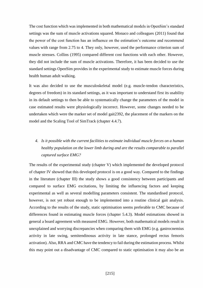
[215]

The cost function which was implemented in both mathematical models in OpenSim’s standard

settings was the sum of muscle activations squared. Monaco and colleagues (2011) found that

the power of the cost function has an influence on the estimation’s outcome and recommend

values with range from 2.75 to 4. They only, however, used the performance criterion sum of

muscle stresses. Collins (1995) compared different cost functions with each other. However,

they did not include the sum of muscle activations. Therefore, it has been decided to use the

standard settings OpenSim provides in the experimental study to estimate muscle forces during

health human adult walking.

It was also decided to use the musculoskeletal model (e.g. muscle-tendon characteristics,

degrees of freedom) in its standard settings, as it was important to understand first its usability

in its default settings to then be able to systematically change the parameters of the model in

case estimated results were physiologically incorrect. However, some changes needed to be

undertaken which were the marker set of model gait2392, the placement of the markers on the

model and the Scaling Tool of SimTrack (chapter 4.4.7).

4. Is it possible with the current facilities to estimate individual muscle forces on a human

healthy population on the lower limb during and are the results comparable to parallel

captured surface EMG?

The results of the experimental study (chapter V) which implemented the developed protocol

of chapter IV showed that this developed protocol is on a good way. Compared to the findings

in the literature (chapter III) the study shows a good consistency between participants and

compared to surface EMG excitations, by limiting the influencing factors and keeping

experimental as well as several modelling parameters consistent. The standardised protocol,

however, is not yet robust enough to be implemented into a routine clinical gait analysis.

According to the results of the study, static optimisation seems preferable to CMC because of

differences found in estimating muscle forces (chapter 5.4.3). Model estimations showed in

general a board agreement with measured EMG. However, both mathematical models result in

unexplained and worrying discrepancies when comparing them with EMG (e.g. gastrocnemius

activity in late swing, semitendinosus activity in late stance, prolonged rectus femoris

activation). Also, RRA and CMC have the tendency to fail during the estimation process. Whilst

this may point out a disadvantage of CMC compared to static optimisation it may also be an

[216]

indication of underlying dynamic inconsistencies which are hidden in the static optimisation

approach due to a lesser sensitivity to it.

Therefore, with this protocol it is not yet possible to estimate individual muscle forces on a

human heathy population of the lower limb. However, the current facilities which are available

may allow to reach this. To be able to do so, more research needs to be undertaken to understand

existing uncertainties and limitations in more detail. Also, these analysis are based on a healthy

population which indicates an exacerbating of these issues in clinical work for patients with a

range of different pathologies. Therefore, the protocol needs also to be tested on patient groups

to make a better statement about the validity of muscle force estimation in clinical gait analysis.

[217]

6.2 Critical Appraisal of Research Design

Some general limitations of the approach of this PhD thesis need to be pointed out.

When choosing OpenSim, the operator needs to accept to be bound to the limitations of this

simulation environment. Although OpenSim has a big user community with which it is possible

to discuss issues about the different tools and models on a provided internet platform, direct

professional help is not provided from the developer. OpenSim is a free available tool, which

may have its advantages as every movement laboratory is able to download the programme

including various musculoskeletal models. However, it may also leave the operator sometimes

in ignorance of important steps which need to be undertaken to run an estimation successfully.

Although SimTrack seems straight forward and applicable without any deep knowledge about

the modelling and simulation process, the operator may struggle to understand every step which

needs to be undertaken to result in decent estimations. OpenSim lives, therefore, from the

contribution of its users. The developer of OpenSim do their best to keep up with up-to-date

user guidelines. A lot of work has been done in the last years to develop the project OpenSim

to a professional tool. Despite the limitations to work with OpenSim it has great possibilities.

To be able to use these possibilities, straight forward protocols are needed which do not need

any subjective interference of the operator. Furthermore, the collaboration with experts in the

fields where the programme with be applied may help to integrate more knowledge about the

need of this profession. This means that for the application into a clinical gait analysis routine,

a close collaborations with clinicians and related researchers is needed. A first step has been

undertaken with this PhD project as the Scaling Tool has been further developed (chapter 4.4.1).

The generic model is scaled in a more anatomical and physiological correct way so that joint

centres and anatomical landmarks are aligned with the skeleton. However, it is to date only

applicable for participants who are able to have their foot flat on the floor during the static

standing trial. This means that this protocol is not suitable for patients like children with cerebral

palsy who are not able to bring their heel down to the floor. Also, the protocol has only been

tested on healthy adults. The results of this thesis are, therefore, only valid for this specific

population group. More research is needed to open this pipeline to a broader population group.

The musculoskeletal model gait2392 has been used in its standard settings (chapter 4.2). One

limitation of this model is that the maximum isometric force defined for each muscle is not

scaled automatically to the participant’s characteristics. It was decided that these standard

settings were accepted for this study. Automatic changes to other muscle-tendon properties

[218]

have not been explored further. Muscle-tendons’ origin and insertion are based on cadaver

studies and, when using the Scaling Tool, are only scaled according to the length of the

segments. This means that moment arms of specific muscles are not adjusted according to the

individual participant. For healthy participants this all may not be from major issue, however,

for patients with restricted neuromuscular functions this presents a major limitation.

One limitation of the mathematical model static optimisation is that it does not include the

activation-contraction cycle. This means that all neurological processes which are involved in

muscle force production are not incorporated. Therefore, static optimisation has its limitations

when estimating muscle forces of patients with neurological diseases (e.g. cerebral palsy,

stroke, or Parkinson’s). However, for musculoskeletal diseases (joint replacements, prosthesis,

and sport injuries) static optimisation may be sufficient. For further studies it may be in general

useful to look first on musculoskeletal diseases before to be able to apply a protocol on

neurological disorders.

The pre-step RRA which needs to be successfully undertaken before CMC is discussable. Joint

angles as well as the centre of mass of the participant’s torso are adjusted to be more consistent

with the experimental GRFs. OpenSim justifies this step to minimise experimental errors

between the camera and the force plate system (which may arise out of slight differences

between the coordinate systems of both measurement systems). However, it is unclear if this

adaptation of joint angles and centre of mass of the torso are physiologically correct or if the

detected error may result out of GRF errors which may change the data in the wrong direction

when applying RRA. Contrary to this, static optimisation may not be sensitive enough to detect

dynamic inconsistencies.

[219]

6.3 Original Contributions and Wider Impact

The novel work within this PhD thesis can be summarised as follows:

1. The systematic review is the first in biomechanical modelling focussing on muscle

forces and joint moments in human healthy walking and summarising graphical material

together in one normalised graph. The review analysed successfully the variability

between muscle force and joint moment profiles across a gait cycle which were

presented in relevant studies. Also, the focus lied on comparing the three main

mathematical models with each other which were used to estimate muscle forces.

The results highlighted a diversity of approaches and results and a need for further

harmonisation and validation. This attributes and adds knowledge to the study of Hicks

and colleagues (2015) who summarised best practise for verification and validation of

musculoskeletal models and simulations of movements. Additionally to the study of

Hicks and colleagues this systematic review could summarise potential influencing

factors on the estimation’s outcome. Therefore, this systematic review could contribute

to the current knowledge of muscle force estimation in clinical movement analysis

which shows the usefulness of such approaches in biomechanical modelling.

2. This study is one of the very few works using recent technology in mathematical

modelling to estimate muscle forces independently of EMG measurements, specifically

in order to be able to validate the shape and speed-dependence with EMG without bias.

This is important as EMG measurements are the only validation tool so far which is able

to present muscle coordination non-invasively. Also, this study used simultaneously

captured EMG data parallel to the kinematics and ground reaction forces which were

used in the modelling process. This ensured a minimal intra- and inter-subject

variability. Most studies which estimated muscle forces and validated the results to

EMG used EMG data also in their estimation process. Furthermore, some studies did

not collect their own EMG data and used available EMG profiles from the literature or

only presented an on-off pattern of captured EMG data (chapter III and chapter V). As

an example, the study of Neptune and colleagues (2008), one of the only studies to

analyse the dependence of walking speed on some of the muscles of the lower limb,

compared the estimated muscle forces to EMG. However, they used these EMG data

into their estimation process, too, to define the muscle excitation patters. Therefore, this

[220]

study could increase the quality of the results compared to other studies by using

independent and simultaneously captured EMG data.

3. This study could contribute to the knowledge of validating two different mathematical

models in terms of whether the simulations show similar changes in

activation/excitation with walking speed as measured EMG at different walking speeds.

The wide and substantial approach of this study is novel compared to existing studies

as it includes more muscles of the lower limb related to walking and compared to

participant-specific EMG measurements. Neptune and colleagues (2008) used an EMG-

driven mathematical model and only present the EMG speed-dependent changes of the

soleus and gastrocnemius which were averaged across all participants included into the

study. Liu and colleagues (2008) used CMC to estimate speed-dependent muscle forces

on children and used averaged EMG standard deviation bands to validate the estimates

muscle forces. Thus, this PhD study could enhance the knowledge about speed-

dependent muscle force estimations by comparing them to independent and participant-

specific EMG and between two mathematical models.

4. Developing the Scaling Tool in the SimTrack pipeline of OpenSim was the first

approach to propose a technique for model scaling and calibration which requires no

intervention from the operator. Also, its marker set definition was adjusted to make it

suitable for clinical purposes. The standard Scaling Tool in OpenSim recommends the

user subjective adjustment of the markers in case scaling errors are too high (Hicks &

Dunne, 2012):

“Frequently, it is helpful to preview the inverse kinematic solution for the

static pose before adjusting the positions of the model markers. This can

be useful for identifying markers that are poorly placed on the model that

you may need to manually adjust or may decide not to include in the

inverse kinematic problem.”

To be able to include such a tool into the clinical gait analysis it is important that the

operator does not need to subjectively interfere into the calculation process as the

repeatability is not given. Therefore, this developed Scaling Tool for the use in OpenSim

could resolve this issue and adjusted the SimTrack pipeline to the needs of the clinical

gait analysis.

5. This study could develop a small normative data pool of muscle force estimation for ten

healthy adults during different walking speeds while systematically comparing the

[221]

mathematical models static optimisation and computed muscle control with each other.

The results will be made available on the OpenSim web-site to enable other OpenSim

users to compare their data with this study. This is very important to motivate the

interaction between different movement laboratories and encourage them to up-load

their data which will develop a big community for estimating muscle forces in clinical

gait analysis.

6. Through conducting this study, important limitations and uncertainties of the current

approaches to estimate muscle activations and forces could be uncovered. These results

showed that this protocol to estimate muscle forces in clinical gait analysis is not yet at

the stage to be implemented into a clinical routine processing. However, the results

which have been found can help to guide future work to be able to make modelling and

simulation accessible for the implementation into the clinical gait analysis. Also, for

slower walking speeds, the results showed better results for both mathematical models,

which might point out that these models are suitable for the purpose of measuring

patients as this population group mostly walks slower than a healthy population.

[222]

6.4 Future Work

One of the major research questions which may be performed to bring the protocol another step

forward is to understand the musculoskeletal model gait2392 in more detail. Standardised

settings like the characteristics of each muscle-tendon complex should be able to be adjusted to

each participant and, especially, to each patient with different disorders. The recent study of

Arnold and colleagues (2013) tested the influence of the muscle-fibre-length and -velocity’s

influence on muscle force estimations at different walking and running speeds, but especially

focused on the walking-to-running transition. They used a musculoskeletal model (A. S. Arnold

et al., 2000) implemented in OpenSim. Their findings suggested for some of the muscles an

increase, but, interestingly, for other muscles a decrease of muscle force generation ability

especially for the plantarflexors. They conclude that the muscle-tendon architecture of these

muscles may not reach the demand for higher walking speeds. There findings show some

limitations of available musculoskeletal models and the need of muscular-tendon characteristics

more adapted to the anthropometrics of the participant.

This means that more studies need to be undertaken to understand if participant specific muscle-

tendon properties may enhance the estimation’s output. Firstly, muscle-tendon settings need to

be systematically changed to understand the behaviour of these and, secondly, a standardised

and straight forward way to adjust muscle-tendons properties automatically need to be

developed. One solution may be magnetic resonance imaging (MRI) with which it is possible

to define the orientation of the muscles to the segments and to calculate the maximum isometric

force a muscle can exert (A. S. Arnold et al., 2000). Some of the muscle-tendon properties have

already been analysed with the help of MRI imaging. Bolsterlee and colleagues (2015) used

MRI to scale physiological cross-sectional area of muscles of the upper limb to analyse the

influence on musculoskeletal model estimations who, however, only showed marginal

differences in the estimation’s output. Bosmans and colleagues (2015) determined individual

origins and insertions of 33 lower limb muscles to analyse the influence on estimated muscle

forces during walking compared to a generic model and found significant changes on the

estimation’s output.

The implementation of MRI scans has already been used in OpenSim as an option for the

scaling of the segments. The disadvantage of this method, however, is that it is not available

for every clinical gait analysis laboratory and is expensive to run. This may suggest two

solutions, either to develop a database for different demographical and physiological

[223]

characteristics (e.g. gender, age, body height, condition of the patient), or to use methods like a

standardised MVC test to account for individual maximal isometric forces.

It is highly important to test the robustness of the study by evaluating the sensibility of the

protocol step by step (Hicks et al., 2015). Some first stage improvements have been done in this

work, especially on the scaling routine of the musculoskeletal model. Influencing factors in the

estimation’s outcome need to be known, understood and controlled. Speed-dependent

differences have been analysed in this study, but other factors can have an influence on the

estimations outcome like other experimental conditions or processing steps of the estimation

routine. These factors need to be analysed in detail to understand their influence on the

estimations’ outcome and to take them if applicable into account. Especially the uncertainties

and limitations which have been detected through the experimental study to estimate muscle

activations and forces need to be analysed to be able to make modelling and simulation tools

more robust for a clinical use.

If the standardised pipeline is developed to a point that uncertainties are understood and

limitations can be taken into account for interpretation purposes, the standardised pipeline needs

to be tested with different marker sets to account for the Conventional Gait Model but also the

6-degree-of-freedom models frequently used in clinical gait analysis, which are slightly

different to the OpenSim marker-set (A. Leardini et al., 2007). Important is as well that the

protocol is tested on a group of participants, and not on single individuals. This is however, to

date rarely the case in the literature, many modelling studies focus on one participant only.

Recent studies like the work of Pinzone and colleagues (Pinzone, Schwartz, & Baker, 2016)

pointed out the high kinematic and kinetic variability which exists between individual

participants during walking. This confirms the need of studies on bigger cohort groups.

Furthermore, this standardised protocol needs to be tested on patients with various conditions

as this work is only based on healthy adult walking which may exacerbate detected issues with

modelling and simulation routines.

[224]

APPENDICIES

A.1 OpenSim: muscle-tendon actuators of model gait2392.

A.2 OpenSim: mass and inertia of gait2392 segments.

A.3 A typical .osim file format for musculoskeletal models in OpenSim.

A.4 Developed Vicon BodyLanguage model to calculate anatomical landmarks and joint

centres.

A.5 Technical development of the scaling in OpenSim.

A.6 Ethical approval.

A.7 Participant information sheet.

A.8 Research participant consent form.

A.9 Rotated vs non-rotated force plates.

[225]

A.1 OpenSim: muscle-Tendon Actuators of model gait2392

Table A.1. Muscle tendon actuators of OpenSim model gait2392.

right left right left

Gluteus Medius 1 819 glut_med1_r glut_med1_l Psoas Major 1113 psoas_r psoas_l

Gluteus Medius 2 573 glut_med2_r glut_med2_l Quadratus Femoris 381 quad_fem_r quad_fem_l

Gluteus Medius 3 653 glut_med3_r glut_med3_l Gemellus 164 gem_r gem_l

Gluteus Minimus 1 270 glut_min1_r glut_min1_l Piriformis 444 peri_r peri_l

Gluteus Minimus 2 285 glut_min2_r glut_min2_l Rectus Femoris 1169 rect_fem_r rect_fem_l

Gluteus Minimus 3 323 glut_min3_r glut_min3_l Vastus Medialis 1294 vas_med_r vas_med_l

Semimembranosus 1288 semimem_r semimem_l Vastus Intermedius 1365 vas_int_r vas_int_l

Semitendinosus 410 semiten_r semiten_l Vastus Lateralis 1871 vas_lat_r vas_lat_l

Biceps Femoris Long Head 896 bifemlh_r bifemlh_l Medial Gastrocnemius 1558 med_gas_r med_gas_l

Biceps Femoris Short Head 804 bifemsh_r bifemsh_l Lateral Gastrocnemius 683 lat_gas_r lat_gas_l

Sartorius 156 sar_r sar_l Soleus 3549 soleus_r soleus_l

Adductor Longus 627 add_long_r add_long_l Tibialis Posterior 1588 tib_post_r tib_post_l

Adductor Brevis 429 add_brev_r add_brev_l Flexor Digitorum Longus 310 flex_dig_r flex_dig_l

Adductor Magnus 1 381 add_mag1_r add_mag1_l Flexor Hallucis Longus 322 flex_hal_r flex_hal_l

Adductor Magnus 2 343 add_mag2_r add_mag2_l Tbibialis Anterior 905 tib_ant_r tib_ant_l

Adductor Magnus 3 488 add_mag3_r add_mag3_l Peroneus Brevis 435 per_brev_r per_brev_l

Tensor Fasciae Latae 233 tfl_r tfl_l Peroneus Longus 943 per_long_r per_long_l

Pectineus 266 pect_r pect_l Peroneus Tertius 180 per_tert_r per_tert_l

Gracilis 162 grac_r grac_l Extensor Digitorum Longus 512 ext_dig_r ext_dig_l

Gluteus Maximus 1 573 glut_max1_r glut_max1_l Extensor Hallucis Longus 162 ext_hal_r ext_hal_l

Gluteus Maximus 2 819 glut_max2_r glut_max2_l Erector Spinae 2500 ercspn_r ercspn_l

Gluteus Maximus 3 552 glut_max3_r glut_max3_l Internal Oblique 900 intobl_r intobl_l

Iliacus 1073 iliacus_r iliacus_l External Oblique 900 extobl_r extobl_l

AbbrevationMuscle actuator Muscle actuator

AbbrevationMax iso

force

Max iso

force

[226]

A.2 OpenSim: mass and Inertia of gait2392 Segments

Table A.2. Mass and inertia of gait2392 segments.

xx yy zz

Torso 34.3266 1.4745 0.7555 1.4314

Pelvis 11.777 0.1028 0.0871 0.0579

Femur 9.3014 0.1339 0.0351 0.1412

Tibia 3.7075 0.0504 0.0051 0.0511

Talus 0.1 0.001 0.001 0.001

Calcaneus 1.25 0.0014 0.0039 0.0041

Toe 0.2166 0.0001 0.0002 0.001

Body

Segment

Mass

(kg)

Moments of Inertia

[227]

A.3 A Typical .osim File Format for Musculoskeletal Models in OpenSim

<?xml version="1.0" encoding="UTF-8" ?>

<OpenSimDocument Version="20303">

<Model name="3DGaitModel2392">

<length_units>meters</length_units>

<force_units>N</force_units>



<gravity> 0 -9.80665 0</gravity>



<BodySet>

<objects>

<Body name="ground">

<mass>0</mass>

<mass_center> 0 0 0</mass_center>

<inertia_xx>0</inertia_xx>

<inertia_yy>0</inertia_yy>

<inertia_zz>0</inertia_zz>

<inertia_xy>0</inertia_xy>

<inertia_xz>0</inertia_xz>

<inertia_yz>0</inertia_yz>



<Joint />

<VisibleObject>



<GeometrySet>

<objects>

<DisplayGeometry>



<geometry_file>treadmill.vtp</geometry_file>



<color> 1 1 1</color>

[228]



<texture_file />



<scale_factors> 1 1 1</scale_factors>



<display_preference>0</display_preference>



<opacity>1</opacity>

</DisplayGeometry>

</objects>

<groups />

</GeometrySet>








<show_axes>false</show_axes>




</VisibleObject>

<WrapObjectSet>

<objects />

<groups />

</WrapObjectSet>

</Body>

…

</objects>

<groups />

</BodySet>

<ForceSet>

[229]

<objects>

<Thelen2003Muscle name="glut_med1_r">



<isDisabled>false</isDisabled>



<min_control>0</min_control>



<max_control>1</max_control>



<GeometryPath>

<PathPointSet>

<objects>

<PathPoint name="glut_med1_r-P1">

<location> -0.0408 0.0304 0.1209</location>

<body>pelvis</body>

</PathPoint>

<PathPoint name="glut_med1_r-P2">

<location> -0.0218 -0.0117 0.0555</location>

<body>femur_r</body>

</PathPoint>

</objects>

<groups />

</PathPointSet>

<VisibleObject>



<GeometrySet>

<objects />

<groups />

</GeometrySet>

[230]



<show_axes>false</show_axes>




</VisibleObject>

<PathWrapSet>

<objects />

<groups />

</PathWrapSet>

</GeometryPath>



<optimal_force>1</optimal_force>



<max_isometric_force>819</max_isometric_force>



<optimal_fiber_length>0.0535</optimal_fiber_length>



<tendon_slack_length>0.078</tendon_slack_length>



<pennation_angle_at_optimal>0.13962634</pennation_angle_at_optimal>



<max_contraction_velocity>10</max_contraction_velocity>



<activation_time_constant>0.01</activation_time_constant>



<deactivation_time_constant>0.04</deactivation_time_constant>



<FmaxTendonStrain>0.033</FmaxTendonStrain>



<FmaxMuscleStrain>0.6</FmaxMuscleStrain>



<KshapeActive>0.5</KshapeActive>



<KshapePassive>4</KshapePassive>

[231]



<Af>0.3</Af>



<Flen>1.8</Flen>

</Thelen2003Muscle>

…

</groups>

</ForceSet>

</Model>

</OpenSimDocument>

[232]

A.4 Developed Vicon BodyLanguage model to calculate anatomical

landmarks and joint centres.

{* Adjust pelvic landmarks *}

PelO = (LASIS + RASIS)/2

PelAPUnit = (PelO - VSacral)/dist(PelO,VSacral)

LeftASIS = LASIS - ($MarkerRadius + $ASISstt)*PelAPUnit

RightASIS = RASIS - ($MarkerRadius + $ASISstt)*PelAPUnit

Sacrum = VSacral + ($MarkerRadius + $PSISstt)*PelAPUnit

output(LeftASIS,RightASIS,Sacrum)

PelvisOrigin = (LeftASIS + RightASIS)/2

output(PelvisOrigin)

{* Calculate Hip joint centres *}

PelvisBB = [PelvisOrigin,(LeftASIS-RightASIS),(PelvisOrigin-Sacrum),yzx]

PX = dist(PelvisOrigin,Sacrum)

PZ = dist(LeftASIS,RightASIS)

RightHipJointCentre = {-0.352*PX,-0.350*PZ,-0.561*PX}*PelvisBB

Output(RightHipJointCentre)

LeftHipJointCentre = {-0.352*PX,0.350*PZ,-0.561*PX}*PelvisBB

Output(LeftHipJointCentre)

{* Calculate midpoint of L and R Acromium *}

MidAcromionPoint = (LAcromium + RAcromium)/2

output(MidAcromionPoint)

[233]

{* Calculate lumbar sacral joint centre *}

LumbarSacralJoint = {-0.808*PX,-0,0.363*PX}*PelvisBB

output(LumbarSacralJoint)

{* Adjust knee landmarks *}

RMKnee = (RKneeLat + RKneeMed)/2

LMKnee = (LKneeLat + LKneeMed)/2

LKneeAxis = (LKneeLat - LKneeMed)/dist(LKneeLat,LKneeMed)

LeftMedialEpicondyle = LKneeMed + ($MarkerRadius + $Kneestt)*LKneeAxis

LeftLateralEpicondyle = LKneeLat - ($MarkerRadius + $Kneestt)*LKneeAxis

Output(LeftMedialEpicondyle,LeftLateralEpicondyle)

RKneeAxis = (RKneeLat - RKneeMed)/dist(RKneeLat,RKneeMed)

RightMedialEpicondyle = RKneeMed + ($MarkerRadius + $Kneestt)*RKneeAxis

RightLateralEpicondyle = RKneeLat - ($MarkerRadius + $Kneestt)*RKneeAxis

Output(RightMedialEpicondyle,RightLateralEpicondyle)

{* Calculate knee joint *}

RightKneeMid = (RightMedialEpicondyle + RightLateralEpicondyle)/2

LeftKneeMid = (LeftMedialEpicondyle + LeftLateralEpicondyle)/2

RightKneeWidth = RightLateralEpicondyle(2) - RightMedialEpicondyle(2)

LeftKneeWidth = LeftLateralEpicondyle(2) - LeftMedialEpicondyle(2)

RightKneeJointFactorX = 100/RightKneeWidth*13

LeftKneeJointFactorX = 100/LeftKneeWidth*13

RightKneeCentreX = RightKneeMid(1)+RightKneeJointFactorX

LeftKneeCentreX = LeftKneeMid(1)-LeftKneeJointFactorX

RightKneeJointCentre = {RightKneeCentreX,RightKneeMid(2),RightKneeMid(3)}

LeftKneeJointCentre = {LeftKneeCentreX,LeftKneeMid(2),LeftKneeMid(3)}

Output(RightKneeJointCentre,LeftKneeJointCentre)

[234]

{* Adjust ankle landmarks *}

RMAnkle = (RAnkleLat + RAnkleMed)/2

LMAnkle = (LAnkleLat + LAnkleMed)/2

LAnkleAxis = (LAnkleLat - LAnkleMed)/dist(LAnkleLat,LAnkleMed)

LeftMedialMalleolus = LAnkleMed + ($MarkerRadius + $Anklestt)*LAnkleAxis

LeftLateralMalleolus = LAnkleLat - ($MarkerRadius + $Anklestt)*LAnkleAxis

Output(LeftMedialMalleolus,LeftLateralMalleolus)

RAnkleAxis = (RAnkleLat - RAnkleMed)/dist(RAnkleLat,RAnkleMed)

RightMedialMalleolus = RAnkleMed + ($MarkerRadius + $Anklestt)*RAnkleAxis

RightLateralMalleolus = RAnkleLat - ($MarkerRadius + $Anklestt)*RAnkleAxis

Output(RightMedialMalleolus,RightLateralMalleolus)

{* Calculate ankle joint *}

RightMidMallPoint = (RightMedialMalleolus + RightLateralMalleolus)/2

LeftMidMallPoint = (LeftMedialMalleolus + LeftLateralMalleolus)/2

RightAnkleJointCentre=RightKneeJointCentre + 1.053*(RightMidMallPoint-RightKneeJointCentre)

LeftAnkleJointCentre=LeftKneeJointCentre + 1.053*(LeftMidMallPoint-LeftKneeJointCentre)

Output(RightAnkleJointCentre,LeftAnkleJointCentre)

{* Calculate ankle joint on ground *}

RightAnkleOnFloor = {RightAnkleJointCentre(1),RightAnkleJointCentre(2),$FloorHeight}

LeftAnkleOnFloor = {LeftAnkleJointCentre(1),LeftAnkleJointCentre(2),$FloorHeight}

Output(RightAnkleOnFloor,LeftAnkleOnFloor)

{* Adjust foot markers on level ground *}

LeftHalluxOnFloor = {LToeTip(1),LToeTip(2),$FloorHeight}

Output(LeftHalluxOnFloor)

RightHalluxOnFloor = {RToeTip(1),RToeTip(2),$FloorHeight}

Output(RightHalluxOnFloor)

[235]

Left5MTPJointOnFloor = {LToeLat(1),LToeLat(2),$FloorHeight}

Output(Left5MTPJointOnFloor)

Right5MTPJointOnFloor = {RToeLat(1),RToeLat(2),$FloorHeight}

Output(Right5MTPJointOnFloor)

Left1MTPJointOnFloor = {LToeMed(1),LToeMed(2),$FloorHeight}

Output(Left1MTPJointOnFloor)

Right1MTPJointOnFloor = {RToeMed(1),RToeMed(2),$FloorHeight}

Output(Right1MTPJointOnFloor)

LeftPosteriorCalcaneusOnFloor = {LHeel(1),LHeel(2),$FloorHeight}

Output(LeftPosteriorCalcaneusOnFloor)

RightPosteriorCalcaneusOnFloor = {RHeel(1),RHeel(2),$FloorHeight}

Output(RightPosteriorCalcaneusOnFloor)

[236]

A.5 Technical Development of the Scaling in OpenSim

Estimated landmark calibration of biomechanical models for inverse

kinematics

Trinler U.1 & Baker R.1

1School of Health Science, University of Salford, United Kingdom

Abstract- Inverse kinematics is emerging as the optimal method in movement analysis to match a multi-

segment biomechanical model to experimental marker positions. Little consideration exists in the literature

for the best approach of this modelling approach. The aim for this study is to propose a generic rational

technique consisting of automated three steps model scaling, static pose estimation and marker calibration

being driven by inverse dynamics. A standard musculoskeletal model of OpenSim has been adapted based

on a process of estimating the position of anatomical landmarks from markers placed on a person during a

static calibration trial. 10 healthy participants were captured in static position and normal walking. Results

showed good results with a mean static and dynamic fitting error of 0.83cm and 0.91cm respectively. All

fitting errors lied under the recommended range except the lateral epicondyle in static pose with a 2.05cm

error. Highest fitting errors were found on the epicondyle (static), feet (static, dynamic) and on the thigh

(dynamic). These may result out of the knee and ankle being designed as a one degree of freedom joint and,

therefore, not being able to account for tibia torsion, and a foot segment without a separate toe segment.

This approach makes it possible to use inverse kinematics in an automated pipeline resulting in good results

for a healthy population. More investigations have to be undertaken for participants outside the normal

range.

Keywords- Inverse kinematics, biomechanical modelling, human movement analysis.

Introduction

Inverse kinematics [1], also known as global optimisation [2] and kinematic fitting, is emerging as the optimal

method for matching a multi-segment biomechanical model to a set of experimental marker positions measured

during movement analysis. The quality of the kinematic fit is dependent on how a generic model of the skeletal

system and the locations of markers upon it is adapted to reflect the anthropometry of the person being measured

and the actual positions of those markers. It involves three interacting processes; scaling (adjusting the dimensions

of the model segments to correspond to those of the person being analysed), fitting (adjusting the pose of the model

to that in which the person is standing) and model marker alignment (specifying the position of markers within the

model to correspond to the measured position of actual markers).

The calibrated anatomical systems technique (CAST) [3] proposed a method for calibrating a six degree of freedom

model of the lower limbs. It only defined segment origins and co-ordinate systems and thus the primary additional

requirement for contemporary biomechanical modelling is to include segment scaling. Most contemporary

[237]

musculoskeletal models are linked segment models requiring further adaptations to the CAST. Currently available

software packages have thus implemented calibration of linked segment models in a number of different ways

(e.g. Visual3d, C-motion Inc, Germantown, MD, USA [4]; OpenSim [5]). OpenSim [5] is becoming more and

more widely used for musculoskeletal modelling and although it includes a Scaling Tool this requires interaction

from the operator to complete full model calibration. Thus a subjective and hence variable process is introduced

into a processing pathway which is otherwise objective and standardised. The paper will thus present an

implementation of the generic technique within OpenSim which using the Scaling Tool in such a way that operator

interaction is not required.

Material and Methods

This is a three stage process operating on data captured during a static calibration trial. In the first the positions of

a number of anatomical landmarks and joint centres are estimated based on the positions of skin mounted

calibration markers. It uses marker locations to estimate the position of bony anatomical landmarks and joint

centres in such a way that scaling and fitting can be performed simultaneously in a manner that is consistent with

the biomechanical model. Anatomical landmarks are estimated on the basis of the measured calibration marker

position, the known dimensions of the marker and an estimate of the soft tissue thickness (STT). In the second the

model is scaled and fitted to the participant to ensure that the anatomical landmarks and joint centres defined within

the model are registered to those estimated from experimental data. Each segment was scaled separately along its

principal axis [6] (longitudinal axis for foot, tibia, femur, thorax and medio-lateral axis for pelvis) and in the plane

perpendicular to that (equally in both directions). Once the model has been scaled it is to minimise a weighted root

mean square of the distances between modelled and measured landmarks and joint centres. The weighted sum is

used to bias the fit in favour of the joint centres. Once the fit has been performed the position of the tracking

markers within the corresponding segment coordinate system as specified in the model is set to match the measured

position of the markers. The process is structured in such a way that the interacting elements of scaling, fitting and

model marker alignment are automatically satisfied without the requirement for any interaction from the operator.

A convenience sample of ten healthy adult volunteers with no history of neuro-musculoskeletal impairments was

recruited from the university community (28±5 years old, 1.72±0.08m, 69±12kg). 38 markers were placed (Table

A.3). A 16 infra-red camera motion capture system (Nexus 1.8.5, Vicon, T40S cameras) was used to capture data

from a static calibration trial (standing upright with feet flat on the floor) and then from several walks at self-

selected walking speed over a walkway with four force plates (Kistler, 2x 9286A, 2x 9253A). The estimated

anatomical landmarks and joint centres for static trial data were calculated using a BodyLanguage model (Vicon,

Oxford, UK) running within Nexus. The hip and lumbar sacral joint centres are estimated to be in a position

consistent with the pelvic segment when scaled along the medio-lateral and anterior-posterior axes to fit the

estimated positions of the ASIS and Sacrum landmarks. Knee and ankle joint centres are estimated to be halfway

between the medial and lateral femoral epicondyle and malleolus landmarks respectively.

Scaling, fitting and model marker alignment was implemented using the OpenSim Scaling Tool and model

3DGaitModel2392 (as distributed with OpenSim 3.2). The location of the key anatomical landmarks within their

respective coordinate systems were estimated from the bone meshes and of the joint centres from the model file

and added to the model as additional markers. Only the estimated landmarks and joint centres (not the original

[238]

marker positions) were used for scaling and fitting. Segments were scaled separately along the principal axis to fit

to joint centres and in the plane perpendicular to this to fit landmark pairs. The only exception to this was at the

foot which was scaled vertically to fit the distance between the ankle joint centre and the floor and in the horizontal

plane to fit the distance between the heel and toe markers. A weighting of 3:1 in favour of the joint centres biased

the fitting of the principal axes to the joint centres leaving the landmark information to determine the rotation of

segments about those axes.

Table A.3 Physical markers used (as listed within GaitModel2392).

Position on body Description

Sternum Placed on the thorax frontal on the sternum.

Acromion Representing the shoulder; placed on the most prominent bony process of the

scapular.

ASIS Anterior superior iliac spine.

VSacral Midpoint between both posterior superior iliac spines.

ThighUpper

ThighFront

ThighRear

Three tracking markers on the thigh, two lateral (upper, rear) and one frontal

(front).

KneeLat Placed on the lateral epicondyle of the femur.

KneeMed Placed on the medial epicondyle of the femur.

ShankUpper

ShankFront

ShankRear

Three tracking markers placed on the shank, two lateral (upper, rear) and one

frontal (front).

AnkleLat Placed on the lateral malleolus.

AnkleMed Placed on the medial malleolus.

Heel Placed on the posterior calcaneus.

MidfootLat

MidfootSup

ToeLat

ToeMed

Four tracking markers placed on the medial and lateral side of the midfoot, and

two markers placed on the medial and lateral side of the forefoot

(metatarsophalangeal joint).

ToeTip Placed on top of the hallux.

Once the model had been scaled the Inverse Kinematics tool was used to fit it to one of the walking trials for each

volunteer. The mean and maximum RMS fitting error calculated across the trial was recorded for both the static

[239]

and walking trials as a measure of the quality of fit of the model to the measurements. For the dynamic trials, skin

mounted markers were used for the kinematic fitting.

Results

Scaling factors for different segments differ slightly between each other as well as between the three directional

scaling axes of some of the segments. Especially on the thigh, the primary axis (y) has been scaled with much

smaller scaling factors compared to the axes normal to the primary axis (x,z). Mean static and dynamic fitting

errors of single relevant joint centres, bony landmarks and skin mounted markers as well as maximum errors

averaged across participants are presented in Table A.4. Overall RMS fitting errors are 0.83cm and 0.91cm for

static and dynamic trials respectively. These values lie in the recommended error range of less than 1cm for static

and 2cm for dynamic trials [7]. Mean RMS fitting errors for the static trial are the lowest at the pelvis, at the joint

centres and at the ankles, which do not exceed 1cm. Fitting errors for the epicondyle landmarks at the knee range

between 1.17 and 2.05cm, with one landmark just over the recommended limit of 2cm (lateral left epicondyle,

2.05cm). Both landmarks on the fifth metatarsal are approximately double as high as the average but still in the

2cm range.

Dynamic RMS fitting errors are in average slightly greater than averaged static errors but the range between 0.65

and 1.14cm is smaller than 0.15 and 2.05cm for the static fitting. Highest mean fitting errors are found at the thighs

and at the tip toes with slightly greater errors than 1cm. RMS maximal fitting errors for the dynamic trials ranging

between 1.37 and 3.02cm, which are all in the recommended maximal value of 2-4cm [7]. Greatest maximal errors

can be found as well at the feet and the thighs.

Table A.4. Mean fitting errors for relevant bony landmarks, joint centres and skin mounted markers of static and

dynamic trials and maximum marker error for the dynamic trial in cm across ten participants.

Static Trial (overall RMS error = 1.06)

Mean

MidAcromium

0.15

LASIS

0.27

RASIS

0.27

Sacrum

0.32

LHJC

0.21

RHJC

0.22

LKJC

0.78

Mean

RKLC

0.65

LEpiconL

2.05

REpiconL

1.95

LEpiconM

1.35

REpiconM

1.17

LAJC

0.43

RAJC

0.46

Mean

LMalleoL

0.98

RMalleoL

0.78

LMalleoM

0.66

RMalleoM

0.61

L5MTP

1.65

R5MTP

1.49

[240]

Dynamic Trial (overall RMS error = 0.91)

Mean

Max

LAcromium

0.82

1.57

RAcromium

0.75

1.41

Sternum

0.85

1.37

LASIS

0.86

1.49

RASIS

0.81

1.57

VSacral

0.65

1.33

RThighF

1.07

1.93

Mean

Max

RThighU

1.15

2.05

RThighR

1.00

2.30

RShankF

0.76

1.87

RShankU

0.87

2.14

RShankR

0.79

2.00

LThighF

1.14

1.82

LThighU

1.19

2.08

Mean

Max

LThighR

1.02

1.78

LShankR

0.82

1.66

LShankU

0.88

2.10

LShankR

0.75

1.82

LHeel

0.85

2.16

RHeel

0.82

2.34

LToeTip

1.12

3.02

Mean

Max

RToeTip

1.14

2.95

LToeLat

1.01

2.66

RToeLat

0.98

2.44

LToeMed

0.76

1.66

RToeMed

0.83

2.71

Discussion

This approach provides a generic and objective technique for the model scaling, static pose estimation and marker

calibration of advanced musculoskeletal models which are driven by inverse kinematics. An automated pipeline

has been conducted consisting of one main algorithm to define the estimated bony landmark and joint centre

positions which then are used in the scaling tool of OpenSim [8].

The more conventional approach to this problem incorporates marker positions instead of landmarks as part of the

model and fits these directly to the measured marker positions. Whilst estimating landmark positions and joint

centres and fitting the model to these appears to introduce an extra step to the process it allows much more control

over exactly how the model is scaled and the static pose determined. The precise method chosen ensures that model

scaling and static pose estimation are mutually consistent.

The scaling factors for the primary axis have been found to be smaller especially for the thigh segment than scaling

factors in both other planes. This may reflect the elderly cadavers on which the model is based on [9], having

narrower bones than the healthy young adults from whom measurements were taken. Such scaling markedly

increases the moment arms of several key muscles at a number of joints. These differences may explain the

recurrent observation that current models do not have the moment generating capacity expected. Moreover, the

visual STT estimation between bones and skin mounted markers could have influenced the scaling in x and z

direction, especially with participants of greater muscle and fatty tissue. With a thicker STT the marker used for

calculating bony landmarks in these both directions would have lied more far away from the bone than expected.

[241]

Including landmark estimation as a separate stage of the process makes the process much more explicit and gives

a clear indication of how methods might need to be adapted in measurements of people where such estimation is

challenging, e.g. such participants with significant soft tissue. Relatively simple measurements of soft tissue

thickness from ultrasound or other approaches, could easily be factored into the algorithms for landmark

estimation. Equally techniques based on indicating landmarks with a wand rather than directly by markers could

also easily be incorporated.

Some marker experienced greater fitting errors than others. The greater RMS fitting errors on the feet may reflect

individual variations of the foot-toe length relation. The musculoskeletal model chosen for this study defined the

foot as one segment and markers placed on the fore foot may be placed on a slight different anatomical landmark

than on the participant when the participant has a different relative length of the toes to the rest of the foot than the

virtual model. The additional higher fitting errors on the epicondyles (static) and on the thighs (dynamic) may

result out of the knee and the ankle being modelled as a single degree of freedom angle. This means, that the model

cannot account for a possible tibia torsion in transversal plane [9].

Although the general principles underlying this approach are applicable to any other study the specific

implementation has limitations. It should only be used for people who are able to stand with their feet flat on the

floor and for whom the required landmarks can be reliably palpated. Modifications to the technique will be required

to make similar measurements for people for whom this is not the case. Further studies may analyse the application

of the proposed technique on other populations than healthy young adults. In conclusion, the presented generic

approach could successfully include a systematic pipeline with which the operator can scale and calibrate the

musculoskeletal model for inverse kinematics automatically.

References

[1] Reinbolt JA, Schutte JF, Fregly BJ, Koh BI, Haftka RT, George AD, et al. Determination of patient-specific

multi-joint kinematic models through two-level optimization. J Biomech. 2005;38:621-6.

[2] Lu TW, O'Connor JJ. Bone postion estimation from skin marker co-ordinates using global optimisation with

joint constraints. Jounrnal of Biomechanics. 1999;32:129-34.

[3] Cappozzo A, Catani F, Croce UD, Leardini A. Position and Orientation in space of bones during movement,

anatomical frame definition and determination. Clinical Biomechanics. 1995;10:171-8.

[4] Hamill J, Selbie WS, Kepple TM. Three-dimensional kinematics. In: Robertson DGE, Caldwell GE, Hamill J,

Kamen G, Whittlesey SN, editors. Research Methods in Biomechanics. Champaign, Il: Human kinetics; 2014.

[5] Delp SL, Anderson FC, Arnold AS, Loen P, Habib A, John CT, et al. OpenSim: Open-Source Software to

Create and Analyze Dynamic Simulations of Movement. IEEE Trans Biomed Eng. 2007;54:1940-50.

[6] Baker R. Globographic visualisation of three dimensional joint angles. J Biomech. 2011;44:1885-91.

[7] OpenSim. OpenSim Support. 2013.

[8] Hicks J, Dunne J. How Scaling Works. OpenSim Documentation2012.

[9] Delp SL, Loan P, Hoy MG, Zajac FE, Topp EL, Rosen JM. An interactive graphics-based model of the lower

extremtiy to study orhtopaedics surgical procedures. IEEE transactions on bio-medical engineering. 1990;37:757-

67.

[242]

A.6 Ethical Approval

[243]

A.7 Participant Information Sheet

Study title

Muscle activity in human movement analysis: Mathematical

modelling vs. surface EMG

This is an invitation to take part in a movement analysis study. Please take time to read this

information sheet thoroughly. If you have any questions, or if you think you might like to take

part in, please do not hesitate to contact me (details below).

If, after reading all the information below, speaking to the researchers, you will be asked to sign

a participant consent form before the measurement. After you have signed the consent form,

you may withdraw from the study at any time, without giving the investigator any reason. In

addition, after the measurement procedure, you can choose to have your data deleted. Your data

will, of course, be handled in confidence.

What is the purpose of this study?

The main purpose of the study is to collect data, which will be used to compare two different

measurement methods during five different movement tasks: a simple movement of one leg

while standing on the other, bending over in standing position, a squat, a vertical jump, and

normal walking. Two different variation factors will be embedded into the measurement tasks:

we will vary the movement tasks in their speed and/ or ask you to wear a weight jacket (which

will be 10% of your body weight) or an ankle weight (one kg heavy) to analyse if speed or

weight have an influence on the measurements.

The measurements taken are, firstly, surface electromyography of the legs (EMG – which

measures whether a muscle is active or not by recording the electrical impulses, sent through

nerves to turn the muscle on) and, secondly, a measures of your movement position and forces

acting on your joints during the movements (via force plates). This will be compared to

mathematical model predictions, where dynamic measured data of the movements will be used

as input.

Am I eligible to take part?

We are inviting all adults who are a staff member or a student at the University of Salford, aged

18 and older, and have no neurological, orthopaedic disease/ injury or other health issues

affecting their legs.

[244]

What do I have to do?

If you choose to take part in this study, we will arrange an appointment at the University of

Salford gait laboratory. The measurement will be a single session of approximately 2 1/2 hours.

During the session, you will be asked to wear shorts and a t-shirt, and to be barefooted. In the

beginning, the researcher will make some anthropometric measurements of you (body height,

weight, length of your legs and the width of your knees and ankles).

The next step will be, to place surface EMG electrodes with a medical tape on your legs, and,

in addition, get them fixed with a bandage. This procedure is painless and the medial tape is

easy to remove later. After this, the electrodes will be tested through maximal voluntary

contractions of your muscles against a resistance, where you will be seated on a chair.

After placing the electrodes, retro-reflective markers will be put on specific positions at your

hip, thigh, shank and feet with medical tape as well. Infra-red cameras positioned around the

room record the position of the reflective markers as you perform the movement tasks (walking,

squatting, vertical jumping, bending forward and knee extension). Force plates (similar to

weight scales), embedded in the floor, will also be used to measure the forces acting on your

body as you perform the movement tasks. We will ask you to repeat each of the movement

three to ten times. If you need a break during the measurement, do not hesitate to ask. During

the different movement tasks there will be brakes anyway.

All the collected data of you will be handled in confidence; none of the camera data records

your personal image. The cameras only record positions of the markers on your body and data

will be labelled with a study ID number and not your name. In this way no one can identify you

or connect your data with your identity. Digital images may be taken from you during standing

or during the exercises, without any identifying features visible, for checking the marker and

electrode placement.

Participating in the measurement is voluntary; you can withdraw without giving us any reason

at any time.

What are the disadvantages or risks of taking part in?

The test only involves walking on an even ground as well as easy exercises, where the risk of

injury is, realistically, very low. The weights, which we will use to modify the movement tasks,

will be fixed safely onto your body. You may become tired during the exercises. Rest brakes

can be taken at any point during the measurement procedure. Should either you or the researcher

have any indication that you may not be able to perform any more movement trials, the study

will be stopped without any consequence to you whatsoever.

What are the advantages in taking part?

We hope that the study will improve our understanding of how muscle activation can be

measured in a patient friendly way and, therefore, how mathematical models can be accurately

used to predict muscle activation without the use of EMG. This information may help clinicians

as well as sport scientists to analyse specific disease pattern or sport movements and develop

new knowledge.

[245]

Will my taking part in this study be kept confidential?

As mentioned above, the acquired data will be kept strictly confidential, no one, except the

investigator and her supervisors, will have access to your data. The data will be stored in a

password protected computer, or will be locked away with no identifying markers whatsoever.

The data will only be used by the primary researcher for her PhD studies.

What will happen to the results of this study?

The results of this study will be used for the PhD work of the investigator and may be used for

presentations at conferences. Neither the presentations nor publications (dissertation,

articles…) will identify individuals who participated in the study.

Contact for problems and questions

If you have any questions or problems about any aspect of this study, contact the researchers at

any time, and they will do their best to answer your questions. You can contact them under the

email address [email protected].

If you still have concerns or complaints you can use the formally way through contacting the

supervisors of the primary researcher, who will follow the University Procedure for Allegations

of Scientific or Ethical Misconduct.

Thank you for reading this!

Ursula Kathinka Trinler, principal investigator

Contact details

Primary researcher: Ursula Trinler ([email protected])

Supervisors: Prof. Richard Baker, Dr. Richard Jones, Dr. Kris Hollands

Information Sheet based on: COREC/NHS National Patient Safety Agency. Information Sheets and Consent Forms – Guidance for Researcher and Reviewers’ Version 3.0 Dec 2006.

Link to IRAS website - IRAS

[246]

A.8 Research Participant Consent Form

Title of Project: Muscle activity in human movement analysis: Mathematic modelling

vs. surface EMG

Ethics Ref No: HSCR13/45

Name of Researcher: Ursula Trinler

(Delete as appropriate)

I confirm that I have read and understood the information

sheet for the above study (version x- date) and what my

contribution will be.

Yes

No

I have been given the opportunity to ask questions (face to face, via

telephone and e-mail)

Yes

No

I agree to digital images being taken during the research exercises

Yes

No

I understand that my participation is voluntary and that I can

withdraw from the research at any time without giving any reason

Yes

No

I understand how the researcher will use my responses, who will see

them and how the data will be stored.

Yes

No

I agree to take part in the above study

Yes

No

Name of

participant

……………………………………………………

Signature

…………………………………………………………

Date ……………………………….

Name of researcher taking consent

Ursula Trinler

[247]

A.9 Results of correcting the Force Plate to the Camera System

A systematic error was detected: the calibration wand was misplaced for about 1-2mm and,

therefore, less than 1° rotated around the origin of the global measurement volume. To analyse

the effect on the results all ten walking trials during self-selected walking speed of the

participant with the greatest centre of mass torso shift (P02) were manually corrected by

aligning the trajectories of the sacrum marker with the centre of pressures of the force plates.

Following figures show the joint moments (Figure A.1), muscle forces estimated with static

optimisation (Figure A.2) and computed muscle control (Figure A.3) of the right leg (left side

resulted in similar results). Figures affected are the hip abduction moment, as well as parts of

the gluteus medius.

Figure A.1. Joint moments of participant P02 before (blue) and after rotating the force plates (red).

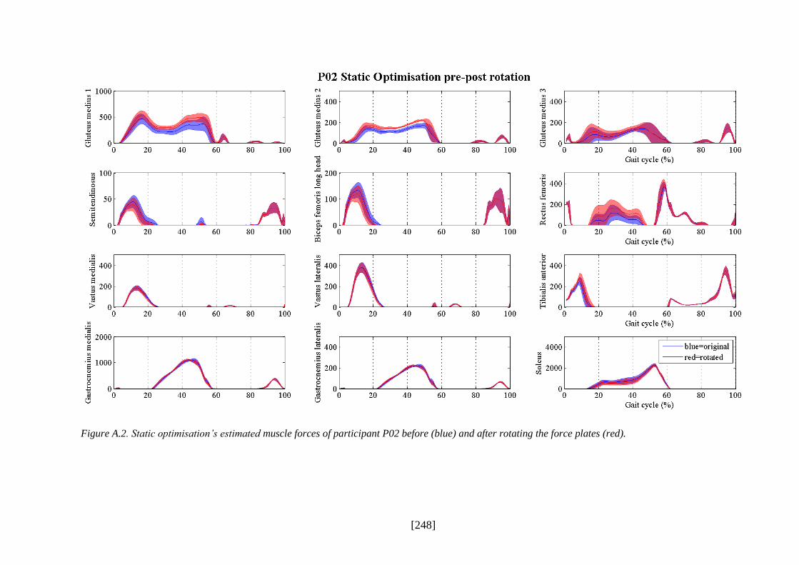
[248]

Figure A.2. Static optimisation’s estimated muscle forces of participant P02 before (blue) and after rotating the force plates (red).

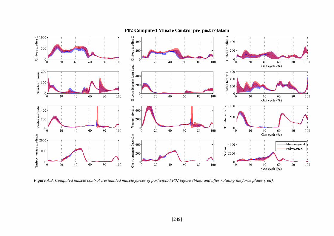
[249]

Figure A.3. Computed muscle control’s estimated muscle forces of participant P02 before (blue) and after rotating the force plates (red).

[250]

List of References

Ackland, D. C., Lin, Y. C., & Pandy, M. G. (2012). Sensitivity of model predictions of muscle

function to changes in moment arms and muscle-tendon properties: a Monte-Carlo

analysis. Journal of Biomechanics, 45(8), 1463-1471.

Alkjaer, T., Simonsen, E., & Dyhre-Poulsen, P. (2001). Comparison of inverse dynamics

calculated by two- and three-dimensional models during walking. Gait and Posture,

13(2), 73-77.

Alkner, B. A., Tesch, P. A., & Berg, H. E. (2000). Quadriceps EMG/force relationship in knee

extension and leg press. Medicine & Science in Sports & Exercise, 32(2), 459-463.

Anderson, F. C., & Pandy, M. G. (1999). A dynamic optimization solution for vertical jumping

in three dimensions. Comput. Meth. Biomech. Biomed. Eng., 2, 201-231.

Anderson, F. C., & Pandy, M. G. (2001a). Dynamic optimization of human walking. J Biomech

Eng, 123(5), 381-390.

Anderson, F. C., & Pandy, M. G. (2001b). Static and dynamic optimization solutions for gait

are practically equivalent. Journal of Biomechanics, 34(2), 153-161. doi:

10.1016/S0021-9290(00)00155-X.

Andriacchi, T. P. (1988). Biomechanics and gait analysis in total knee replacement. Orthop

Rev, 17(5), 470-473.

Andriacchi, T. P., & Alexander, E. J. (2000). Studies of human locomotion: past, present,

future. Journal of Biomechanics, 33(10), 1217-1224.

Arch, E. S., Stanhope, S. J., & Higginson, J. S. (2015). Passive-dynamic ankle-foot orthosis

replicates soleus but not gastrocnemius muscle function during stance in gait: Insights

for orthosis prescription. Prosthet Orthot Int. doi: 10.1177/0309364615592693.

Arnold, A. S., Anderson, F. C., Pandy, M. G., & Delp, S. L. (2005). Muscular contributions to

hip and knee extension during the single limb stance phase of normal gait: a framework

for investigating the causes of crouch gait. Journal of Biomechanics, 38(11), 2181-2189.

[251]

Arnold, A. S., Salinas, S., Asakawa, D. J., & Delp, D. (2000). Accuracy of Muscle Moment

Arms Estimated from MRI-Based Musculoskeletal Models of the Lower Extremity.

Computer Aided Surgery, 5, 108-119.

Arnold, E. M., Hamner, S. R., Seth, A., Millard, M., & Delp, S. L. (2013). How muscle fiber

lengths and velocities affect muscle force generation as humans walk and run at

different speeds. J Exp Biol, 216(Pt 11), 2150-2160. doi: 10.1242/jeb.075697.

Arnold, E. M., Ward, S. R., Lieber, R. L., & Delp, S. L. (2010). A Model of the Lower Limb

for Analysis of Human Movement. Annals of Biomedical Engineering, 38(2), 269-279.

Au, C., & Dunne, J. (2012, 09.08.2013). Gait 2392 and 2354 Models. OpenSim Documentation.

Retrieved 08.02.2015, from http://simtk-confluence.stanford.edu:8080/display/

OpenSim/Gait+2392+and+2354+Models.

Baker, R. (2007). The history of gait analysis before the advent of modern computers. Gait

& Posture, 26(3), 331-342. doi: 10.1016/j.gaitpost.2006.10.014.

Baker, R. (2011). Globographic visualisation of three dimensional joint angles. J Biomech,

44(10), 1885-1891. doi: 10.1016/j.jbiomech.2011.04.031.

Baker, R. (2013). Measuring Malking: A Handbook of Clinical Gait Analysis. London:

MacKeith Press.

Basmajian, J. V., & De Luca, C. J. (1985). Muscles Alive. Their Functions Revealed by

Electromyography (5th ed.). Baltimore, USA: Williams & Wilkins.

Bazett-Jones, D. M., Cobb, S. C., Joshi, M. N., Cashin, S. E., & Earl, J. E. (2011). Normalizing

hip muscle strength: establishing body-size-independent measurements. Arch Phys Med

Rehabil, 92(1), 76-82. doi: 10.1016/j.apmr.2010.08.020.

Besier, T., Fredericson, M., Gold, C., Beaupre, G., & Delp, S. L. (2009). Knee muscle forces

during walking and running in patellofemoral pain patients and pain-free controls.

Journal of Biomechanics, 42(7), 898-905.

Bigland, B., & Lippold, O. C. J. (1954). The relation between force, velocity and integrated

electrical activity in human muscles. Journal of Physiology, 123, 214-224.

Blackburn, J. T., Bell, D. R., Norcross, M. F., Hudson, J. D., & Engstrom, L. A. (2009).

Comparison of hamstring neuromechanical properties between healthy males and

[252]

females and the influence of musculotendinous stiffness. J Electromyogr Kinesiol,

19(5), e362-369. doi: 10.1016/j.jelekin.2008.08.005.

Bogey, R. A., Cerny, K., & Mohammed, O. (2003). Repeatability of wire and surface electrodes

in gait. Am J Phys Med Rehabil, 82(5), 338-344. doi:

10.1097/01.PHM.0000064717.90796.7A.

Bogey, R. A., Gitter, A. J., & Barnes, L. A. (2010). Determination of ankle muscle power in

normal gait using an EMG-to-force processing approach. Journal of Electromyography

and Kinesiology, 20(1), 46-54. doi: http://dx.doi.org/10.1016/j.jelekin.2008.09.013.

Bogey, R. A., Perry, J., & Gitter, A. J. (2005). An EMG-to-Force Processing Approach for

Determining Ankle Muscle Forces During Normal Human Gait. IEEE Transactions on

Neural Systems and Rehabilitation Engineering, 13(3), 302-310.

Bohannon, R. W., & Williams Andrews, A. (2011). Normal walking speed: a descriptive meta-

analysis. Physiotherapy, 97(3), 182-189. doi: 10.1016/j.physio.2010.12.004.

Bolsterlee, B., Vardy, A. N., van der Helm, F. C., & Veeger, H. E. (2015). The effect of scaling

physiological cross-sectional area on musculoskeletal model predictions. J Biomech,

48(10), 1760-1768. doi: 10.1016/j.jbiomech.2015.05.005.

Bosmans, L., Valente, G., Wesseling, M., Van Campen, A., De Groote, F., De Schutter, J., &

Jonkers, I. (2015). Sensitivity of predicted muscle forces during gait to anatomical

variability in musculotendon geometry. J Biomech, 48(10), 2116-2123. doi:

10.1016/j.jbiomech.2015.02.052.

Bowsher, K. A., & Vaughan, C. L. (1995). Effect of foot-progression angle on hip joint

moments during gait. Journal of Biomechanics, 28(6), 759-762.

Brand, R. A., Crowninshield, R., Wittstock, C., Pedersen, D., Clark, C., & van Krieken, F.

(1982). A Model of Lower Extremity Muscular Anatomy. JOurnal of Biomechanical

Engineering, 104, 304-310.

Brand, R. A., Pedersen, D. R., & Friedrich, J. A. (1986). The Sensitivity of Muscle Force

Predictions to Changes in Physiologic Cross-Sectional Area. Journal of Biomechanics,

19(8), 589-596.

Bresler, B., & Frankel, J. P. (1950). The forces and Moments in the Leg During Level Walking.

Trans. ASME, 72, 27-36.

[253]

Buchanan, T. S., Lloyd, D. G., Manal, K., & Besier, T. F. (2005). Estimation of Muscle Forces

and Joint Moments Using a Forward-Inverse Dynamics Model. Medicine & Science in

Sports & Exercise, 37(11), 1911-1916.

Burden, A. (2010). How should we normalize electromyograms obtained from healthy

participants? What we have learned from over 25 years of research. J Electromyogr

Kinesiol, 20(6), 1023-1035. doi: 10.1016/j.jelekin.2010.07.004.

Cappozzo, A., Catani, F., Croce, U. D., & Leardini, A. (1995). Position and Orientation in space

of bones during movement, anatomical frame definition and determination. Clinical

Biomechanics, 10, 171-178.

Chand, J., Hammer, S., & Hicks, J. (2012, 14.11.2014). Collecting Experiemntal Data.

OpenSim Documentation. Retrieved 11.02.2015, from http://simtk-

confluence.stanford.edu:8080/display/OpenSim/Collecting+Experimental+Data.

Chandler, R., Clauser, C., McConville, J., Reynolds, H., & Young, J. (1975). Investigation of

the inertial properties of the human body. Springfield, Virgina.

Chow, C. K., & Jacobson, D. H. (1971). Human Locomotion via Optimal Programming.

Mathemactical Bioscience, 10, 239-306.

Clarys, J. (2000). Electromyography in sports and occupational settings: an update of its limits

and possibilities. Ergonomics, 43, 1750-1762.

Collins, J. J. (1995). The redundant nature of locomotor optimization laws. Journal of

Biomechanics, 28(3), 251-267.

Crowninshield, R. D., & Brand, R. A. (1981). A physiologically based criterion of muscle force

prediction in locomotion. Journal of Biomechanics, 14(11), 793-801. doi:

10.1016/0021-9290(81)90035-X.

Davis III, R. B., Õunpuu, S., Tyburski, D., & Gage, J. R. (1991). A gait analysis data collection

and reduction technique. Human Movement Science, 10(5), 575-587. doi:

10.1016/0167-9457(91)90046-Z.

De Groote, F., Pipeleers, G., Jonkers, I., Demeulenaere, B., Patten, C., Swevers, J., & De

Schutter, J. (2009). A physiology based inverse dynamic analysis of human gait:

potential and perspectives. Computer Methods in Biomechanics & Biomedical

Engineering, 12(5), 563-574.

[254]

De Leva, P. (1996). Adjustments to Zatsiorsky-Seluyanov's segment intertia parameters.


De Luca, C. J. (1997). The Use of Surface Electromyography in Biomechanics. Journal of

Applied Biomechanics, 13(2), 135-163.

Della Croce, U., Leardini, A., Chiari, L., & Cappozzo, A. (2005). Human movement analysis

using stereophotogrammetry. Part 4: assessment of anatomical landmark misplacement

and its effects on joint kinematics. Gait Posture, 21(2), 226-237. doi:

10.1016/j.gaitpost.2004.05.003.

Delp, S. L. (1990). Surgery Simulation: A Computer Graphics System to Analyse and Design

Musculoskeletal Reconstructions of the Lower Limb. (Ph.D.), Standford University,

Stanford, CA.

Delp, S. L., Anderson, F. C., Arnold, A. S., Loen, P., Habib, A., John, C. T., . . . Thelen, D. G.

(2007). OpenSim: Open-Source Software to Create and Analyze Dynamic Simulations

of Movement. IEEE Trans Biomed Eng, 54(11), 1940-1950.

Delp, S. L., Arnold, A. A., Speers, R. A., & Moore, C. (1996). Hamstrings and psoas lenths

during normal and crouch gait: implications for muscle-tendon surgery. Journal of

Orthopaedic Research, 14, 144-151.

Delp, S. L., Loan, P., Hoy, M. G., Zajac, F. E., Topp, E. L., & Rosen, J. M. (1990). An

interactive graphics-based model of the lower extremtiy to study orhtopaedics surgical

procedures. IEEE transactions on bio-medical engineering, 37, 757-767.

Delp, S. L., & Maloney, W. (1993). Effects of Hip Center Location on the Moment-Generating

Capacity of the Muscles. Journal of Biomechanics, 26(4/5), 485-499.

Dempster, W. (1955). Space Requirements of the Seated Operator. Geometrical, Kinematic,

and Mechanical Aspects of the BodyWith Special Reference to the Limbs. Wright-

Patterson Air Force Base, OH: Wright Air Development Center, Air Research and

Development Command.

DeVita, P. (2005). Musculoskeletal Modeling and the Prediction of In Vivo Muscle and Joint

Forces. Medicine & Science in Sports & Exercise, 37(11), 1909-1910.

Dixon, P. C., Böhm, H., & Döderlein, L. (2012). Ankle and midfoot kinetics during normal

gait: A multi-segment approach. Journal of Biomechanics, 45(6), 1011-1016.

[255]

Downs, S. H., & Black, N. (1998). The feasibility of creating a checklist for the assessment of

the methodological quality both of randomised and non-randomised studies of health

care interventions. J Epidemiol Community Health, 52, 377-284.

Eng, J. J., & Winter, D. A. (1995). Kinetic analysis of the lower limbs during walking: what

information can be gained from a three-dimensional model? Journal of Biomechanics,

28(6), 753-758.

Erdemir, A., McLean, S., Herzog, W., & van den Bogert, A. J. (2007). Model-based estimation

of muscle forces exerted during movements. Clinical Biomechanics, 22(2), 131-154.

Faber, G. S., Kingma, I., Martin Schepers, H., Veltink, P. H., & van Dieen, J. H. (2010).

Determination of joint moments with instrumented force shoes in a variety of tasks.


Ferrari, A., Benedetti, M., Pavan, E., Frigo, C., Bettinelli, D., Rabuffetti, M., . . . Leardini, A.

(2008). Quantitative comparison of five current protocols in gait analysis. Gait and

Posture, 28(2), 207-216.

Finni, T., Komi, P. V., & Lukkarimiemi, J. (1998). Achulles tendon loading during walking:

application of a novel optic ffiber technique. Eur J Appl Physiol, 77, 289-291.

Fluit, R., van der Krogt, M. M., van der Kooij, H., Verdonschot, N., & Koopman, H. F. (2012).

A simple controller for the prediction of three-dimensional gait. J Biomech, 45(15),

2610-2617. doi: 10.1016/j.jbiomech.2012.08.019.

Fraysse, F., Dumas, R., Cheze, L., & Wang, X. (2009). Comparison of global and joint-to-joint

methods for estimating the hip joint load and the muscle forces during walking. Journal

of Biomechanics, 42(14), 2357-2362.

Friederich, J. A., & Brand, R. A. (1990). Muscle fiber architecture in the human lower limb.


Gage, J. R. (1994). The role of gait analysis in the treatment of cerebral palsy. J Pediatr Orthop,

14(6), 701-702.

Ganley, K., & Powers, C. (2004). Determination of lower extremity anthropometric parameters

using dual energy X-ray absorptiometry: the influence on net joint moments during gait.

Clin Biomech (Bristol, Avon), 19(1), 50-56.

[256]

Glitsch, U., & Baumann, W. (1997). The three-dimensional determination of internal loads in

the lower extremity. Journal of Biomechanics, 30(11–12), 1123-1131. doi:

10.1016/S0021-9290(97)00089-4.

Goldberg, S. R., Kepple, T. M., & Stanhope, S. J. (2009). In Situ Calibration and Motion

Capture Transformation Optimization Improve Instrumented Treadmill Measurements.

Journal of Applied Biomechanics, 25, 401-446.

Gonzales, R., Buchanan, T., & Delp, S. (1997). How muscles architecture and moment arms

affect wrist flexion-extension moments. Jounral of Biomechanics, 30(7), 705-712.

Gordon, A., Huxley, A., & Julian, F. (1966). the variation in isometric tension with sarcomere

length in vertebrate muscle fibres. Jounral of Physiology, 184, 170-192.

Gorton, G. E., 3rd, Hebert, D. A., & Gannotti, M. E. (2009). Assessment of the kinematic

variability among 12 motion analysis laboratories. Gait Posture, 29(3), 398-402. doi:

10.1016/j.gaitpost.2008.10.060.

Grabiner, M., Feuerbach, J., Lundin, T., & Davis, B. (1995). Visual guidance to force plates

does not influence ground reaction froce variability. Journal of Biomechanics, 28(9),

1115-1117.

Grosset, J. F., Piscione, J., Lambertz, D., & Perot, C. (2009). Paired changes in

electromechanical delay and musculo-tendinous stiffness after endurance or plyometric

training. Eur J Appl Physiol, 105(1), 131-139. doi: 10.1007/s00421-008-0882-8.

Hase, K., & Yamazaki, N. (1997). Development of a Three-Dimensional Whole Body

Musculoskeletal Model for Various Motion Analysis. Jsme International Journal Series

C-Dynamics Control Robotics Design and Manufacturing, 40(1), 25-32.

Havanan, E. (1964). A Mathematical Model of the Human Body (pp. 64-102). Ohio: Aerospace

Medical Division.

Heintz, S., & Gutierrez-Farewik, E. M. (2007). Static optimization of muscle forces during gait

in comparison to EMG-to-force processing approach. Gait and Posture, 26(2), 279-288.

Hermens, H., & Freriks, B. Retrieved 25.09.2015, from http://www.seniam.org/.

Hermens, H., Freriks, B., Disselhorst-Klug, C., & Rau, G. (2000). Development of

recommendations for SEMG sensors and sensor placement procedures. Journal of

Electromyographyand Kinesiology, 10, 361-374.

[257]

Herzog, W. (1998). Muscle. In B. M. Nigg & W. Herzog (Eds.), Biomechanics of the Musculo-

skeletal System (Vol. 2nd, pp. 148-188). West Sussex, UK: John Wiley & Sons Ltd.

Hicks, J. (2012a). How Inverse Dynamics Works. Retrieved 13.09.2015, from http://simtk-

confluence.stanford.edu:8080/display/OpenSim/How+Inverse+Dynamics+Works.

Hicks, J. (2012b). Model Editing. OpenSim Support. Retrieved 18.08.2015, 2015, from

http://simtk-confluence.stanford.edu:8080/x/S4Qz.

Hicks, J. (2013, 22.07.2013). OpenSim's Capabilities. OpenSim Documentation. Retrieved

11.02.2015, from http://simtk-confluence.stanford.edu:8080/display/OpenSim/

OpenSim%27s+Capabilities.

Hicks, J., & Dembia, C. (2012, 17.07.2013). How Inverse Kinematics Works. OpenSim

Documentation. Retrieved 11.02.2015, from http://simtk-

confluence.stanford.edu:8080/display/OpenSim/How+Inverse+Kinematics+Works.

Hicks, J., & Dembia, C. (2014). How Static Optimisation Works. Retrieved 13.09.2015, from

http://simtk-confluence.stanford.edu:8080/display/OpenSim/How+Static+

Optimization+Works.

Hicks, J., & Dunne, J. (2012, 14.02.2014). How Scaling Works. OpenSim Documentation.

Retrieved 08.02.2015, from http://simtk-confluence.stanford.edu:8080/pages/viewinfo.

action?pageId=3376178.

Hicks, J., & Uchida, T. (2013a). How CMC Works. Retrieved 15.09.2015, from http://simtk-

confluence.stanford.edu:8080/display/OpenSim/How+CMC+Works.

Hicks, J., & Uchida, T. (2013b). How RRA works. Retrieved 14.09.2015, from http://simtk-

confluence.stanford.edu:8080/display/OpenSim/How+RRA+Works.

Hicks, J., Uchida, T. K., Seth, A., Rajagopal, A., & Delp, S. L. (2015). Is my model good

enough? Best practices for verification and validation of musculoskeletal models and

simulations of movement. J Biomech Eng, 137(2), 020905. doi: 10.1115/1.4029304

Higgins, J., & Green, S. (2011). Cochrane Handbook for Systematic Reviews of Interventions

Retrieved from Available from www.cochrane-handbook.org.

Hill, A. V. (1938). The heat of shortening and the dynamic constrants of muscle. Proceedings

of The Royal Society of London. Series B, 76, 136-195.

[258]

Hill, A. V. (1952). The mechanics of active muscle. Proceedings of the Royal Society of London

- Series B, 141(902), 104-117.

Hof, A. L., Elzinga, H., Grimmius, W., & Halbertsma, J. P. K. (2002). Speed dependence of

averaged EMG profiles in walking. Gait & Posture, 16, 78-86.

Hof, A. L., & van den Berg, J. (1977). Linearity between the weighted sum of the EMGs of the

human triceps surae and the total torque. Journal of Biomechanics, 10, 529-539.

Hollands, K. L., Pelton, T. A., Tyson, A. F., Hollands, M. A., & van Vliet, P. M. (2012).

interventions for coordination of walking following stroke: systematic review. Gait &

Posture, 35, 349-359.

Holloway, C. S., Symonds, A., Suzuki, T., Gall, A., Smitham, P., & Taylor, S. (2015). Linking

wheelchair kinetics to glenohumeral joint demand during everyday accessibility

activities. Conf Proc IEEE Eng Med Biol Soc, 2478-2481.

Hoy, M. G., Zajac, F. E., & Gordon, M. E. (1990). A musculoskeletal model of the human

lower extremity: the effect of muscle, tendon, and moment arm on the moment.angle

relationship of musculotendon actuators at the hip, knee, and ankle. Journal of

Biomechanics, 23(2), 157-169.

Hug, F., Hodges, P. W., & Tucker, K. (2015). Muscle force cannot be directly inferred from

muscle activation: illustrated by the proposed imbalance of force between the vastus

medialis and vastus lateralis in people with patellofemoral pain. J Orthop Sports Phys

Ther, 45(5), 360-365. doi: 10.2519/jospt.2015.5905.

Hughes, V. A., Frontera, W. R., Wood, M., Evans, W. J., Dallal, G. E., Roubenoff, R., &

Fiatarone Singh, M. A. (2001). Longitudinal Muscle Strength Changes in Older Adults:

Influence of Muscle Mass, Physical Activity, and Health. Journal of Gerontology,

56A(5), B209-B217.

Inman, V. (1953). The Pattern of Muscular Activity in the Lower Extremity during Walking:

University of California.

Ivanenko, Y., Dominici, N., & Lacquaniti, F. (2007). Development of Independent Walking in

Toddlers. Exercise and Sport Sciences Reviews, 35(2), 67-73.

Izquierdo, M., Aguado, X., Gonzalez, R. V., López, J. L., & Häkkinen, K. (1999). Maximal and

explosive force production capacity and balance performance in men of different ages.

Eur J Appl Physiol, 79, 260-267.

[259]

Johnson, J. C. (1978). Comparison of analysis techniques for electromyographic data. Aviation

Space & Environmental Medicine, 49, 14-18.

Judge, J. O., Ounpuu, S., & Davis, R. B., 3rd. (1996). Effects of age on the biomechanics and

physiology of gait. Clin Geriatr Med, 12(4), 659-678.

Kadaba, M. P., Ramakrishnan, H. K., & Wootten, M. E. (1990). Measurement of Lower

Extremity Kinematics During Level Walking. Journal Of Orthopaedic Research, 8,

383-392.

Kadaba, M. P., Ramakrishnen, H. K., Wootten, J. G., Gainey, J., Gorton, G., & Cochran, G. V.

B. (1989). Repeatability of Kinematic, Kinetic, and Electromyographic Data in Normal

Adult Gait. Journal Of Orthopaedic Research, 7, 849-860.

Kainz, H., Modenese, L., Carty, C., & Lloyd, D. (2014). Direct kinematics versus inverse

kinematics: Kinematic modelling approach alters lower limb joint kinematics, muscle

moment arm and muscle-tendon length estimates in children with cerebral palsy. Paper

presented at the Congress of the International Society of Electrophysiology and

Kinesiology, Rome, Italy.

Kerrigan, D. C., Todd, M. K., & Della Croce, U. (1998). Gender differences in joint

biomechanics during walking - Normative study in young adults. American Journal of

Physical Medicine & Rehabilitation, 77(1), 2-7. doi: 10.1097/00002060-199801000-

00002.

Kirtley, C. (2006). Clinical gait analysis: theory and practise: Churchill Livingstone,

ELSEVIER.

Kirtley, C., Whittle, M. W., & Jefferson, R. J. (1985). Influence of walking speed on gait

parameters. Journal of Biomedical Engineering, 7, 282-288.

Knutson, D. (2007). Mechanics of the Musculoskeletal System. In D. Knutson (Ed.),

Fundamentals of Biomechanics (pp. 69-103). New York, USA: Springer.

Komi, P. V. (1990). Relevance of in-vivo force measurements to human biomechanics. Journal

of Biomechanics, 23 (Suppl. 1), 23-34.

Komi, P. V., & Viitasalo, J. T. (1967). Signal characteristics of EMG at different levels of

muscle tensions. Acta Physiol Scand, 96, 267-276.

[260]

Komura, T., & Nagano, A. (2004). Evaluation of the influence of muscle deactivation on other

muscles and joints during gait motion. Journal of Biomechanics, 37(4), 425-436. doi:

10.1016/j.jbiomech.2003.09.022.

Komura, T., Nagano, A., Leung, H., & Shinagawa, Y. (2005). Simulating pathological gait

using the enhanced linear inverted pendulum model. IEEE Transactions on Biomedical

Engineering, 52(9), 1502-1513.

Koopman, B., Grootenboer, H. J., & de Jongh, H. J. (1995). An inverse dynamics model for the

analysis, reconstruction and prediction of bipedal walking. Journal of Biomechanics,

28(11), 1369-1376.

Leardini, A., & O'Connor, J. J. (2002). A model for lever-arm length calculation of the flexor

and extensor muscles at the ankle. Gait & Posture, 15(3), 220.

Leardini, A., Sawacha, Z., Paolini, G., Ingrosso, S., Nativo, R., & Benedetti, M. G. (2007). A

new anatomically based protocol for gait analysis in children. Gait Posture, 26(4), 560-

571. doi: 10.1016/j.gaitpost.2006.12.018.

Lee, S., & Son, J. (Producer). (2010, 07.02.2015). Lee-Son's Toolbox: a Toolbox that Converts

VICON Mocap Data into OpenSim Inputs. Retrieved from https://simtk.org/home/lee-

son/.

Lee, S. J., & Hidler, J. (2008). Biomechanics of overground vs. treadmill walking in healthy

individuals. J Appl Physiol, 104, 747-755. doi: 10.1152/japplphysiol.01380.2006.

Lelas, J. L., Merriman, G. J., Riley, P. O., & Kerrigan, D. C. (2003). Predicting peak kinematic

and kinetic parameters from gait speed. Gait & Posture, 17(2), 106-112. doi:

10.1016/s0966-6362(02)00060-7.

Lerner, Z. F., Board, W. J., & Browning, R. C. (2015). Pediatric obesity and walking duration

increase medial tibiofemoral compartment contact forces. J Orthop Res. doi:

10.1002/jor.23028.

Lieber, R. L. (2010). Skeletal Muscle Structure, Function, and Plasticity. The Physiological

Basis of Rehabilitation. (Vol. 3). Philadelphia, USA: Lippincott Williams & Williams.

Lin, Y. C., Dorn, T. W., Schache, A. G., & Pandy, M. G. (2012). Comparison of different

methods for estimating muscle forces in human movement. Proceedings of the

Institution of Mechanical Engineers. Part H - Journal of Engineering in Medicine,

226(2), 103-112.

[261]

Lippold, O. C. J. (1952). The relation between integrated action potentials in a human muscle

and its isometric tension. Journal of Physiology, 117, 492-499.

Liu, J., & Lockhart, T. (2006). Comparison of 3D joint moments using local and global inverse

dynamics approaches among three different age groups. Gait and Posture, 23(4), 480-

485.

Liu, M. Q., Anderson, F. C., Pandy, M. G., & Delp, S. L. (2006). Muscles that support the body

also modulate forward progression during walking. Journal of Biomechanics, 39(14),

2623-2630. doi: 10.1016/j.jbiomech.2005.08.017.

Liu, M. Q., Anderson, F. C., Schwartz, M. H., & Delp, S. L. (2008). Muscle contributions to

support and progression over a range of walking speeds. Journal of Biomechanics,

41(15), 3243-3252. doi: 10.1016/j.jbiomech.2008.07.031.

Lloyd, D. G., & Besier, T. F. (2003). An EMG-driven musculoskeletal model to estimate

muscle forces and knee joint moments in vivo. J Biomech, 36(6), 765-776. doi:

10.1016/s0021-9290(03)00010-1.

Lund, K., & Hicks, J. (2013). Getting Started with RRA. Retrieved 09.10.2015, from

http://simtk-confluence.stanford.edu:8080/display/OpenSim/Getting+Started+

with+RRA.

MacIntosh, B. J., Gardiner, P. F., & MacComas, A. J. (2006). Skeletal Muslce: Form and

Function (2nd ed.): Human Kinetics.

Mahlknecht, P., Kiechl, S., Bloem, B. R., Willeit, J., Scherfler, C., Gasperi, A., . . . Seppi, K.

(2013). Prevalence and burden of gait disorders in elderly men and women aged 60-97

years: a population-based study. PLoS One, 8(7), e69627. doi:

10.1371/journal.pone.0069627.

McConville, J., Clauser, C., Churchill, T., Cuzzi, J. R., & Kaleps, I. (1980). Anthropometric

relationships of bod yand body segment moments of inertia. Wright-Patterson AFB,

Ohio: Air Force Aerospace Medical Research Laboratory.

McGinley, J. L., Baker, R., Wolfe, R., & Morris, M. E. (2009). The reliability of the three-

dimensional kinematic gait measurements: A systematic review. Gait & Posture, 29,

360-369.

[262]

McGinley, J. L., Wolfe, R., Morris, M., Pandy, M., & Baker, R. (2014). Variability of Walking

in Able-Bodied Adults Across Different Time Intervals. Journal of Physical Medicine

and Rehabilitation Sciences, 17, 6-10.

Merletti, R., & Hermens, H. (2000). Introduction to the special issue on the SENIAM European

Concerted Action. Journal of Electromyography and Kinesiology, 10(5), 283-286.

Miller Buffinton, C., Buffinton, E. M., Bieryla, K. A., & Pratt, J. E. (2016). Biomechanics of

Step Initiation After Balance Recovery With Implications for Humanoid Robot

Locomotion. Journal of Biomechanical Engineering, 138(3).

Monaco, V., Coscia, M., & Micera, S. (2011). Cost function tuning improves muscle force

estimation computed by static optimization during walking 33rd Annual International

Conference of the IEEE EMBS, 8263 - 8266.

Murray, M. P., Drought, A. B., & Kory, R. C. (1964). Walking Patterns of Normal Men. Journal

of Bone and Joint Surgery, 46A, 335-360.

Muybridge, E. (1907). The Human Figure In Motion 1907 (third ed. Vol. 3rd impression):

Chapman and Hall.

Nene, A., Byrne, C., & Hermens, H. (2004). Is rectus femoris really a part of quadriceps?:

Assessment of rectus femoris function during gait in able-bodied adults. Gait &

Posture, 20(1), 1-13. doi: 10.1016/s0966-6362(03)00074-2.

Neptune, R. R., & Hull, M. L. (1999). A theoretical analysis of preferred pedaling rate selection

in endurance cycling. Journal of Biomechanics, 32, 409-415.

Neptune, R. R., Kautz, S. A., & Zajac, F. E. (2001). Contributions of the individual ankle plantar

flexors to support, forward progression and swing initiation during walking. Journal of

Biomechanics, 34, 1387-1398.

Neptune, R. R., Sasaki, K., & Kautz, S. A. (2008). The effect of walking speed on muscle

function and mechanical erergetics. Gait & Posture, 28, 135-143.

Nisell, R., Németh, G., & Ohlsén, H. (1986). Joint forces in extension of the knee. Analysis of

a mechanical model. Acta Orthop Scand, 57, 41-46.

Nordez, A., Gallot, T., Catheline, S., Guével, A., Cornu, C., & Hug, F. (2009).

Electromechanical delay revised using very high frame rate ultrasound. J Appl Physiol,

106, 1970-1975. doi: 10.1152/japplphysiol.00221.2009.

[263]

Oggero, E., Pagnacco, G., Morr, D., Simon, S., & Berme, N. (1998). PProbability od valid gait

data acquisition using currently available force plates. Biomedical Sciences

Instrumentation, 34, 392-397.

OpenSim. (2013, 24th of July, 2013). OpenSim Support. 2013, from http://simtk-

confluence.stanford.edu:8080/display/OpenSim/OpenSim+Support.

Pandy, M. G., & Andriacchi, T. P. (2010). Muscle and Joint Function in Human Locomotion.

In M. L. Yarmush, J. S. Duncan & M. L. Gray (Eds.), Annual review of biomedical

engineering (Vol. 12, pp. 401-433).

Pandy, M. G., & Berme, N. (1988a). A numerical method for simulating the dynamics of human

walking. Journal of Biomechancis, 21(12), 1043-1051.

Pandy, M. G., & Berme, N. (1988b). Synthesis of human walking: a planar model for single

support. Journal of Biomechanics, 21(12), 1053-1060.

Pandy, M. G., Zajac, F. E., Sim, E., & Levine, W. S. (1990). An optimal control model for

maximum-height human jumping. Journal of Biomechanics, 23(12), 1185-1198.

Passmore, E., & Sangeux, M. (2014). Improving repeatability of setting volume origin and

coordinate system for 3D gait analysis. Gait Posture, 39(2), 831-833. doi:

10.1016/j.gaitpost.2013.11.002

Perry, J. (1992). Gait nalysis: Normal and Pathological Function. Thorofare, NJ: SLACK

Incorporated.

Perry, J., & Burnfield, J. M. (2010). Gait Analysis: Normal and Pathological Function. 2nd

edition: SLACK incorporated.

Peters, A., Galna, B., Sangeux, M., Morris, M., & Baker, R. (2010). Quantification of soft tissue

artifact in lower limb human motion analysis: A systematic review. Gait & Posture, 31,

1-8.

Piazza, S., & Delp, S. L. (1996). The influence of muscles on the knee flexion during the swing

phase of gait. Journal of Biomechanics, 29(6), 723-733.

Pinzone, O., Schwartz, M. H., & Baker, R. (2016). Comprehensive non-dimensional

normalization of gait data. Gait & Posture, 44, 68-73. doi:

10.1016/j.gaitpost.2015.11.013.

[264]

Prince, F., Corriveau, H., Hébert, R., & Winter, D. A. (1997). Gait in elderly. Gait and Posture,

5, 128-135.

Rabuffetti, M., & Crenna, P. (2004). A modular protocol for the analysis of movement in

children. Gait & Posture ESMAC Abstracts 2004, 20S, S61-S112.

Rampichini, S., Ce, E., Limonta, E., & Esposito, F. (2013). Effects of fatigue on the

electromechanical delay components in gastrocnemius medialis muscle. Eur J Appl

Physiol. doi: 10.1007/s00421-013-2790-9.

Rao, G., Amarantini, D., Berton, E., & Favier, D. (2006). Influence of body segments’

parameters estimation models on inverse dynamics solutions during gait. Journal of

Biomechanics, 39(8), 1531-1536.

Ren, L., Jones, R. K., & Howard, D. (2008). Whole body inverse dynamics over a complete

gait cycle based only on measured kinematics. J Biomech, 41(12), 2750-2759. doi:

10.1016/j.jbiomech.2008.06.001.

Ridgewell, E., Dobson, F., Bach, T. M., & Baker, R. (2010). A systematic review to determine

best practice reporting guidelines for AFO interventions in studies involving children

with cerebral palsy. Prothetics and Orthotics International, 34(2), 129-145.

Rodrigo, S. E., Ambrósio, J. A. C., Tavares da Silva, M. P., & Penisi, O. H. (2008). Analysis

of Human Gait Based on Multibody Formulations and Optimization Tools. Mechanics

Based Design of Structures and Machines, 36(4), 446-477. doi:

10.1080/15397730802425497.

Sartori, M., Reggiani, M., Farina, D., & Lloyd, D. G. (2012). EMG-driven forward-dynamic

estimation of muscle force and joint moment about multiple degrees of freedom in the

human lower extremity. PLoS One, 7(12), e52618. doi: 10.1371/journal.pone.0052618.

Schache, A. G., Baker, R., & Vaughan, C. L. (2007). Differences in lower limb transverse plane

joint moments during gait when expressed in two alternative reference frames. J

Biomech, 40(1), 9-19. doi: 10.1016/j.jbiomech.2005.12.003.

Schuenke, M., Schulte, E., Ross, L. M., Schumacher, U., & Lamperti, E. D. (2006). Atlas of

Anatomy: General Anatomy and Musculosceletal System. Stuttgart: Georg Thieme

Verlag.

Schwartz, M. H., Rozumalski, A., & Trost, J. P. (2008). The effect of walking speed on the gait

of typically developing children. Journal of Biomechanics, 41, 1639-1650.

[265]

Schwartz, M. H., Trost, J. P., & Wervey, R. A. (2004). Measurement and management of errors

in quantitative gait data. Gait Posture, 20(2), 196-203. doi:

10.1016/j.gaitpost.2003.09.011.

Seireg, A., & Arvikar, R. J. (1973). A mathematical model for evaluation of forces in lower

extremities of the musculo-skeletal system. Journal of Biomechanics, 6, 313-326.

Seth, A., & Pandy, M. G. (2007). A neuromusculoskeletal tracking method for estimating

individual muscle forces in human movement. Journal of Biomechanics, 40, 356-366.

Shewman, T., & Konrad, P. (2011). Surface Electromyography (SEMG). Clinical Sequence

assessments and SEMG feedback: A Beginner's Guide. Scottsdale, Arizona USA:

Noraxon U.S.A.

Silva, M. P. T., & Ambrosio, J. A. C. (2003). Solution of redundant muscle forces,in human

locomotion with multibody dynamics and optimization tools. Mechanics Based Design

of Structures and Machines, 31(3), 381-411. doi: 10.1081/sme-120022856.

Sinclair, J., Taylor, P. J., & Hobbs, S. J. (2013). Digital filtering of three-dimensional lower

extremity kinematics: an assessment. J Hum Kinet, 39, 25-36. doi: 10.2478/hukin-2013-

0065.

Skalshoi, O., Iversen, C. H., Nielsen, D. B., Jacobsen, J., Mechlenburg, I., Soballe, K., &

Sorensen, H. (2015). Walking patterns and hip contact forces in patients with hip

dysplasia. Gait Posture, 42(4), 529-533. doi: 10.1016/j.gaitpost.2015.08.008.

Soderberg, G. L., & Cook, T. M. (1984). Electromyography in Biomechanics. Physical

Therapy, 64, 1813-1820.

Spector, S. A., Gardiner, P. F., Zernicke, R. F., Roy, R. R., & Edgerton, V. R. (1980). Muscle

Architecture and Force-Velocity Characteristics of Cat Soleus and Medial

Gastrocnemius: Implications for Motor Control. Journal of Neurophysiology, 44(5),

951-960.

Sutherland, D. H. (1978). Gait analysis in cerebral palsy. Dev Med Child Neurol, 20(6), 807-

813.

Sutherland, D. H. (2001). The evolution of clinical gait analysis part l: kinesiological EMG.

Gait & Posture, 14(1), 61-70. doi: 10.1016/S0966-6362(01)00100-X.

[266]

Szczerbik, E., & Kalinowska, M. (2011). The influence of knee marker placement error on

evaluation of gait kinemaitc parameters. Acta of BIomengineering and Biomechanics,

13(3), 43-46.

Thacker, B. H. (2001). ASME Standards Comittee on Verification and Validation in

Computational Solid Mechanisms Technical Report: ASME Council on Codes and

Standards.

Thelen, D. G. (2003). Adjustment of Muscle Mechanics Model Parameters to Simulate

Dynamic Contractions in Older Adults. Journal of Biomechanical Engineering, 125(1),

70. doi: 10.1115/1.1531112.

Thelen, D. G., Anderson, A. E., & Delp, S. L. (2003). Gererating dynamic simulations of

movement using computed muscle control. Journal of Biomechanics, 36, 321-328.

Thelen, D. G., & Anderson, F. C. (2006). Using computed muscle control to generate forward

dynamic simulations of human walking from experimental data. J Biomech, 39(6),

1107-1115. doi: 10.1016/j.jbiomech.2005.02.010.

Thelen, D. G., Chumanov, E. S., Hoerth, D. M., Best, T. M., Swanson, S. C., Li, L. I., . . .

Heiderscheit, B. C. (2005). Hamstring Muscle Kinematics during Treadmill Sprinting.

Medicine & Science in Sports & Exercise, 37(1), 108-114. doi:

10.1249/01.mss.0000150078.79120.c8.

Umberger, B. R. (2008). Effects of suppressing arm swing on kinematics, kinetics, and

energetics of human walking. J Biomech, 41(11), 2575-2580. doi:

10.1016/j.jbiomech.2008.05.024.

van den Bogert, A. J., & De Koning, J. J. (1996). On optimal filtering for inverse dynamics

analysis. Paper presented at the Proceedings of the IXth Biennial Conference of the

Canadian Society for Biomechanics, Vancouver.

Vaughan, C., Davis, B., & O'Connor, J. (1992). Dynamic of Human Gait. . Champaign, Illinois:

Human Kinetics Publishers.

Vaughan, C., Davis, B. L., & O'Connor, J. C. (1999). Dynamics of Human Gait. Second edition.

Howard Place: Kiboho Publisher.

Verghese, J., LeValley, A., Hall, C. B., Katz, M. J., Ambrose, A. F., & Lipton, R. B. (2006).

Epidemiology of Gait Disorders in Communitx-Residing Older Adults. J Am Geriatric

Soc, 54(2), 255-261.

[267]

Verniba, D., Vergara, M. E., & Gage, W. H. (2015). Force plate targeting has no effect on

spatiotemporal gait measures and their variability in young and healthy population. Gait

Posture, 41(2), 551-556. doi: 10.1016/j.gaitpost.2014.12.015.

White, S. C., & Winter, D. A. (1993). Predicting Muscle Forces in Gait from EMG Signals and

Musculotendon Kinematics. Journal of Electromyography and Kinesiology, 2(4), 217-

231.

Whittle, M. W. (2001). Gait analysis: an introduction (3 ed.): Butterworth-Heinemann.

Wickiewicz, T. L., Roy, R. R., Powell, P. L., & Edgerton, V. R. (1983). Muscle architecture of

the human lower limb. Clin Orthop Relat Res, 179, 275-283.

Winter, D. A. (1990). The Biomechanics and Motor Control of Human Gait: Normal, Elderly

and Pathological: Waterloo Biomechanics.

Winter, D. A. (2009). Biomechanics and motor contral of human movement. 4th edition.

Winter, D. A., Patla, A. E., Frank, J. S., & Walt, S. E. (1990). Biomechanical walking pattern

changes in the fit and healthy elderly. Physical Therapy, 70, 340-347.

Woods, J. J., & Bigland Ritchie, B. (1983). Linear and nonlinear surface EMF/ force

relationships in human muscles: an anatomical/ functional argument for the existence

of both. American Journal of Physical Medicine, 62, 287-299.

Woolf, A. D., Erwin, J., & March, L. (2012). The need to address the burden of musculoskeletal

conditions. Best Pract Res Clin Rheumatol, 26(2), 183-224. doi:

10.1016/j.berh.2012.03.005.

Xu, H., Merryweather, A., Bloswick, D., Mao, Q., & Wang, T. (2015). The effect of toe marker

placement error on joint kinematics and muscle forces using OpenSim gait simulation.

Biomed Mater Eng, 26 Suppl 1, S685-691. doi: 10.3233/BME-151360.

Yamaguchi, G. T., & Zajac, F. E. (1989). A planar model of the knee joint to characterize the

knee extensor mechanism. Journal of Biomechanics, 22(1), 1-10.

Yavuz, S. U., Sendemir-Urkmez, A., & Turker, K. S. (2010). Effect of gender, age, fatigue and

contraction level on electromechanical delay. Clin Neurophysiol, 121(10), 1700-1706.

doi: 10.1016/j.clinph.2009.10.039.

Zajac, F. E. (1989). Muscle and Tendon: Properties, Models, Scaling, and Application to

Biomechanics and Motor Control. Critical Reviews in Biotechnology, 17, 359-411.

[268]

Zatsiorsky, V., Seluyanov, V., & Chugunova, L. (1990). Methonds of determining mass-inertia

characteristics of human body segments. In G. Chernyi & S. Regirer (Eds.),

Contemporary Problems of Biomechanics (pp. 272-291). Massachusetts: CRC Press.

muscle force estimation in clinical gait analysisusir.salford.ac.uk/id/eprint/39257/1/muscle force...

Documents