murphy, neil (2012) estimating the incidence of hiv in sub...
TRANSCRIPT

Glasgow Theses Service http://theses.gla.ac.uk/
Murphy, Neil (2012) Estimating the incidence of HIV in Sub-Saharan Africa. MSc(R) thesis. http://theses.gla.ac.uk/2885/ Copyright and moral rights for this thesis are retained by the author A copy can be downloaded for personal non-commercial research or study, without prior permission or charge This thesis cannot be reproduced or quoted extensively from without first obtaining permission in writing from the Author The content must not be changed in any way or sold commercially in any format or medium without the formal permission of the Author When referring to this work, full bibliographic details including the author, title, awarding institution and date of the thesis must be given

Estimating the Incidence of
HIV in Sub-Saharan Africa
Neil Murphy
A Dissertation Submitted to the
University of Glasgow
for the degree of
Master of Science
School of Mathematics and Statistics
September 2011
c⃝Neil Murphy

Abstract
It is common knowledge that HIV is a serious problem in South Africa
and one of the worst affected areas of this country is KwaZulu-Natal. As
such, accurate measurement of HIV incidence in this area is of vital impor-
tance. Unfortunately, surveys of HIV incidence in the area often return high
numbers of missing results making the task of estimating the incidence and
prevalence very difficult. In this study, methods are developed to produce
accurate measurements of the incidence of HIV from data which contain a
large number of missing values.
As well as developing our own method, we consider the merits of existing
methods of estimating HIV incidence, particularly those which are able to
produce incidence estimates using cross-sectional surveys. These methods
make use of the optical density (OD) value, a measure which can be taken at
the same time as HIV tests and which increases with time since HIV infection.
The OD values are used to ascertain whether HIV-positive individuals are
recently infected or not (i.e. infected within a pre-determined time frame).
These recency classifications are then used to produce estimates of the HIV
incidence.
The method of incidence estimation developed in this study consists of
i

imputing the missing data values before applying traditional methods of in-
cidence estimation to the imputed dataset. This imputation consists of two
parts: deterministic and probabilistic imputation. To impute deterministi-
cally, we assume that once an individual has tested positive for HIV they can-
not then test negative in a later test. This allows us to back- and forward-fill
as appropriate some of the missing values in HIV tests carried out at different
times on the same individual. Remaining missing values are imputed prob-
abilistically with probabilities calculated using observed values in the data.
Using our method, our best estimate of the HIV incidence between the
first and second stage of testing is 31.04 infections per 1000 person years with
a 95% confidence interval of 30.25 to 31.83 infections per 1000 person years.
Our best estimate of the HIV incidence between the second and third stages
of testing is 30.92 infections per 1000 person years with a 95% confidence
interval of 29.72 to 32.13 infections per 1000 person years. Our method also
produces a best estimate of the HIV incidence between the first and third
stages of testing of 30.96 infections per 1000 person year with a 95% confi-
dence interval of 30.46 to 31.47 infections per 1000 person years.
Simulation of HIV test data allows us to assess the accuracy and appro-
priateness of the methods considered in this study. The inclusion of missing
data in these simulated datasets allows us to check the performance of each of
these methods under conditions similar to those seen in our original dataset.
Our imputation method was shown to cope well with missing data and pro-
duced estimates of the incidence with consistently low biases and root mean
square errors. One of the methods which produces incidence estimates based
on cross-sections of the data was also shown to perform reasonably well with
ii

generally good levels of accuracy.
iii

Acknowledgements
I would like to thank my project supervisors Professor John McColl and
Dr Duncan Lee for their help and support throughout this project. My
thanks also go to Till Barnighausen at the Africa Centre for Health and
Population studies for providing the data used in the project. I would also
like to extend my gratitude to the School of Mathematics and Statistics at
the University of Glasgow for funding this research.
Further thanks go to my friends and family for their support and under-
standing throughout the duration of this project.
iv

Contents
1 Introduction 1
1.1 About HIV/AIDS . . . . . . . . . . . . . . . . . . . . . . . . . 1
1.2 The Africa Centre . . . . . . . . . . . . . . . . . . . . . . . . . 2
1.3 Aims of this Study . . . . . . . . . . . . . . . . . . . . . . . . 4
2 Methods and Literature 6
2.1 The Simplest Method of Incidence Estimation . . . . . . . . . 6
2.1.1 Estimating incidence . . . . . . . . . . . . . . . . . . . 6
2.2 Taking time into account when estimating incidence . . . . . . 7
2.3 A few problems . . . . . . . . . . . . . . . . . . . . . . . . . . 9
2.4 Current methods of HIV incidence estimation . . . . . . . . . 10
2.4.1 Parekh’s Incidence Formula . . . . . . . . . . . . . . . 11
2.4.2 McDougal’s Incidence Formula . . . . . . . . . . . . . 14
2.5 Missing Data Mechanisms . . . . . . . . . . . . . . . . . . . . 16
2.6 Missing Data Imputation . . . . . . . . . . . . . . . . . . . . . 17
2.7 Confidence Intervals using Imputed Data Sets . . . . . . . . . 18
2.8 Data Simulation . . . . . . . . . . . . . . . . . . . . . . . . . . 20
2.8.1 Bias . . . . . . . . . . . . . . . . . . . . . . . . . . . . 20
2.8.2 Root Mean Squared Error . . . . . . . . . . . . . . . . 21
2.9 Our intended approach to HIV incidence estimation . . . . . . 22
v

3 Preliminary Analysis 23
3.1 Missing Data . . . . . . . . . . . . . . . . . . . . . . . . . . . 23
3.2 A Crude Method of Incidence estimation . . . . . . . . . . . . 27
3.3 Taking time into account when estimating incidence . . . . . 32
3.4 Applying the Formula Derived in Parekh et al. (2002) to our
Data . . . . . . . . . . . . . . . . . . . . . . . . . . . . . . . . 33
3.4.1 Applying Parekh’s formula to the same data used in
sections 3.2 and 3.3 . . . . . . . . . . . . . . . . . . . . 33
3.4.2 Applying Parekh’s formula to an expanded dataset . . 38
3.4.3 Applying McDougal’s methods of incidence estimation
to our data . . . . . . . . . . . . . . . . . . . . . . . . 39
4 Imputation of Missing Values 41
4.1 Missing Values in our Data Set . . . . . . . . . . . . . . . . . 41
4.2 Deterministic Imputation of HIV Status . . . . . . . . . . . . 41
4.3 Probabilistic Imputation . . . . . . . . . . . . . . . . . . . . . 45
5 Data simulation 55
5.1 Simulating Demography . . . . . . . . . . . . . . . . . . . . . 58
5.2 Simulating HIV test results . . . . . . . . . . . . . . . . . . . 59
5.2.1 Simulating time between tests . . . . . . . . . . . . . . 59
5.2.2 Simulating HIV status at each of the testing stages . . 59
5.2.3 Simulating Recency status . . . . . . . . . . . . . . . . 62
5.3 Missingness . . . . . . . . . . . . . . . . . . . . . . . . . . . . 64
5.3.1 Missing completely at random . . . . . . . . . . . . . . 64
5.3.2 Missing at random . . . . . . . . . . . . . . . . . . . . 65
5.4 Calculate incidence estimates . . . . . . . . . . . . . . . . . . 66
5.5 Impute missing values . . . . . . . . . . . . . . . . . . . . . . 66
vi

5.6 Calculate incidence estimates . . . . . . . . . . . . . . . . . . 66
5.7 MCAR Simulations . . . . . . . . . . . . . . . . . . . . . . . . 67
5.8 MAR Simulations . . . . . . . . . . . . . . . . . . . . . . . . . 71
5.8.1 MAR simulation with 2 age groups . . . . . . . . . . . 71
5.8.2 MAR simulation with 3 age groups . . . . . . . . . . . 74
5.8.3 MAR simulation with 4 Age groups . . . . . . . . . . . 77
5.8.4 MAR simulation with low HIV prevalence and incidences 80
5.8.5 MAR simulation with small sample size . . . . . . . . . 84
5.9 Brief summary of our simulation results . . . . . . . . . . . . . 87
6 Conclusions 89
6.1 Summary of results . . . . . . . . . . . . . . . . . . . . . . . . 89
6.2 Limitations of the study . . . . . . . . . . . . . . . . . . . . . 92
6.3 Further Work . . . . . . . . . . . . . . . . . . . . . . . . . . . 94
Appendices 96
A Additional multiple imputation results 96
B Additional MCAR simulation results 102
B.1 MCAR simulation with 2 age groups . . . . . . . . . . . . . . 102
B.2 MCAR simulation with 4 age groups . . . . . . . . . . . . . . 104
vii

List of Tables
3.1 Number of missing values for variables in data . . . . . . . . . 24
3.2 Table of HIV Status by HIV Status at Previous Stage . . . . . 26
3.3 Missing test results as a proportion by age-sex group (%) . . . 27
3.4 Crude Incidence Estimates for Different Stages of the Study . 29
3.5 Incidence Estimates for Different Stages of the Study using
time between HIV Tests . . . . . . . . . . . . . . . . . . . . . 33
3.6 Incidence Estimates for Different Stages of the Study using
Parekh’s Final Method . . . . . . . . . . . . . . . . . . . . . . 37
3.7 Incidence Estimates for Different Stages of the Study using
Parekh’s intermediate Method . . . . . . . . . . . . . . . . . . 38
3.8 Incidence Estimates for expanded dataset using Parekh’s Meth-
ods . . . . . . . . . . . . . . . . . . . . . . . . . . . . . . . . . 39
3.9 Table of HIV incidence estimates at different stages using dif-
ferent McDougal formulae . . . . . . . . . . . . . . . . . . . . 40
4.1 Table of HIV Status by HIV Status at Previous Stage . . . . . 43
4.2 Crude HIV Incidence estimates before and after deterministic
imputation . . . . . . . . . . . . . . . . . . . . . . . . . . . . . 44
4.3 Missing test results as a proportion by age-sex group after
deterministic imputation (%) . . . . . . . . . . . . . . . . . . 45
4.4 Table of sequences of HIV status after deterministic imputation 46
viii

4.5 Table of possible test result sequences for missing value sequences 47
4.6 Table of age-group breakdowns by number of age-groups . . . 49
4.7 Incidence estimates from multiple imputation using 4 age groups
(infections per 1000 person years) . . . . . . . . . . . . . . . . 52
4.8 Incidence estimates with 95% confidence intervals after multi-
ple imputation (infections per 1000 person years) . . . . . . . 54
5.1 Arbitrarily chosen stage 1 HIV prevalences for different age-
sex groups . . . . . . . . . . . . . . . . . . . . . . . . . . . . . 60
5.2 MCAR probabilities of missingness example . . . . . . . . . . 65
5.3 MAR probabilities of missingness example . . . . . . . . . . . 66
5.4 Simulated HIV prevalences (%) and incidences (infections per
1000 person years) - MCAR simulation with 3 age groups . . . 68
5.5 Simulated probabilities of missingness (%) - MCAR simulation
with 3 age groups . . . . . . . . . . . . . . . . . . . . . . . . . 68
5.6 Bias and RMSE from simulation with imputation . . . . . . . 70
5.7 Simulated HIV prevalences (%) and incidences (infections per
1000 person years) - MAR simulation with 2 age groups . . . . 72
5.8 Probabilities of missingness by stage and age-sex group (%) -
MAR simulation with 2 age groups . . . . . . . . . . . . . . . 73
5.9 Bias and RMSE from simulation with imputation - MAR sim-
ulation with 2 age groups . . . . . . . . . . . . . . . . . . . . . 74
5.10 Simulated HIV prevalences (%) and incidences (infections per
1000 person years) - MAR simulation with 3 age groups . . . . 75
5.11 Probability of missingness by stage and age-sex group (%) -
MAR simulation with 3 age groups . . . . . . . . . . . . . . . 76
5.12 Bias and RMSE from simulation with imputation . . . . . . . 77
ix

5.13 Simulated HIV prevalences (%) and incidences (infections per
1000 person years) - MAR simulation with 4 age groups . . . . 78
5.14 Probabilities of missingness by stage and age-sex group (%) -
MAR simulation with 4 age groups . . . . . . . . . . . . . . . 79
5.15 Bias and RMSE from simulation with imputation . . . . . . . 80
5.16 Simulated HIV prevalences (%) and incidences (infections per
1000 person years) - MAR simulation with low incidences . . . 81
5.17 Probabilities of missingness by stage and age-sex group (%) -
MAR simulation with low incidences . . . . . . . . . . . . . . 82
5.18 Bias and RMSE from simulation with imputation (Simulation
with low incidence and prevalence) . . . . . . . . . . . . . . . 83
5.19 Simulated HIV prevalences (%) and incidences (infections per
1000 person years) - MAR simulation with small sample size . 84
5.20 Probabilities of missingness by stage and age-sex group (%) -
MAR simulation with small sample size . . . . . . . . . . . . . 85
5.21 Bias and RMSE from simulation with imputation (MAR sim-
ulation with small sample size) . . . . . . . . . . . . . . . . . 86
A.1 Incidence estimates from multiple imputation without age group-
ing (infections per 1000 person years) . . . . . . . . . . . . . . 97
A.2 Incidence estimates from multiple imputation using 2 age groups
(infections per 1000 person years) . . . . . . . . . . . . . . . . 98
A.3 Incidence estimates from multiple imputation using 3 age groups
(infections per 1000 person years) . . . . . . . . . . . . . . . . 99
A.4 Incidence estimates from multiple imputation using 5 age groups
(infections per 1000 person years) . . . . . . . . . . . . . . . . 100
A.5 Incidence estimates from multiple imputation using 6 age groups
(infections per 1000 person years) . . . . . . . . . . . . . . . . 101
x

B.1 Simulated HIV prevalences (%) and incidences (infections per
1000 person years) - MCAR simulation with 2 age groups . . . 102
B.2 Bias and RMSE from simulation with imputation . . . . . . . 103
B.3 Simulated HIV prevalences (%) and incidences (infections per
1000 person years) - MCAR simulation with 4 age groups . . . 104
B.4 Bias and RMSE from simulation with imputation . . . . . . . 105
xi

List of Figures
2.1 Flow Diagram of Recency Classification . . . . . . . . . . . . . 13
3.1 Histograms of Time between HIV Tests at different Stages . . 31
5.1 Flow Diagram of Simulation Method . . . . . . . . . . . . . . 57
xii

Chapter 1
Introduction
1.1 About HIV/AIDS
The Human Immunodeficiency Virus (HIV) is a retrovirus which attacks
the cells of the immune system before limiting or preventing their ability
to function, thereby weakening the infected person’s immune system. It is
transmitted by sexual intercourse, transfusion of contaminated blood or by
sharing of contaminated needles. It can also be transmitted from a mother
to her baby during pregnancy, childbirth and breastfeeding. It usually takes
between 10 and 15 years for HIV to reach its final stage which is known as
Acquired Immune Deficiency Syndrome (AIDS). As the virus worsens, the
infected person’s immune system continues to weaken, leaving them vulner-
able to infection from other viruses and diseases.
In 2005, the estimated prevalence of HIV in KwaZulu-Natal was 13.8%
(95% confidence interval (C.I.) 10.3% to 18.2%) for males and 18.5% (95%
C.I. 15.4% to 22.0%) for females (HIV and AIDS Strategy for the Province
of KwaZulu-Natal 2006-2010 (2006)). The estimated overall prevalence for
1

CHAPTER 1. INTRODUCTION 2
both males and females was 16.5% (95% C.I. 14.0% to 19.3%). The HIV
prevalence in the whole of South Africa was estimated as 10.8% so it would
appear that the HIV epidemic is worse in KwaZulu-Natal than it is in other
parts of the country.
Another worrying figure is the estimate in National HIV and Syphilis
Antenatal Sero-Prevalence Survey in South Africa 2004 (2005) that 40.7%
of pregnant women attending antenatal clinics in KwaZulu-Natal were HIV
positive (95% C.I. 38.8% to 42.7%). The same estimate for South Africa as
a whole is 29.5% (95% C.I. 28.5% to 30.5%).
The HIV epidemic in South Africa as a whole is obviously severe and
these figures would suggest that KwaZulu-Natal is one of the worst affected
regions of the country.
1.2 The Africa Centre
Established in 1997 by the University of KwaZulu-Natal and the South
African Medical Research Council with funding from the UK based charity
the Wellcome Trust, the Africa Centre was created to conduct and support
research into issues surrounding the population and reproductive health of
people in sub-Saharan Africa.
Originally named the Africa Centre for Population Studies and Repro-
ductive health, its name was changed in 2002 to the Africa Centre for Health
and Population Studies to signify the wider range of research which is carried
out there. The Centre is located in the Umkhanyakude district of KwaZulu-

CHAPTER 1. INTRODUCTION 3
Natal which is in the grip of an HIV epidemic.
The largest venture being undertaken by the Africa Centre is the Africa
Centre Demographic Information System (ACDIS). This is a demographic
surveillance system (DSS) established in a rural South African population
by the Africa Centre which began data collection on 1 January 2000. The
ACDIS demographic surveillance area is approximately 430km2, contains
about 11,000 households and is located in the southern area of the Umkhanyakude
district of KwaZulu-Natal. In order to be included in the study, an individual
must be a member of a household within the area. What differentiates the
ACDIS from other DSSs is that an individual does not have to be resident
in the surveillance area at the time of data collection as long as they are a
member of a household in the area. Also, unlike other DSSs, individuals can
be a member of more than one household within the area. Given that many
residents of this area often travel to other parts of the country for work, and
so may not be present when data is collected, this allows for collection of
data which give a more accurate representation of the demography of the
area.
As part of the ACDIS, a population-based HIV cohort study was carried
out between 2003 and 2006. To be eligible for inclusion in the cohort, indi-
viduals had to be resident in the surveillance area and aged 15-49 years for
women or 15-54 years for men.
The data in the ACDIS is collected by visiting a key member of each
household every six months who provides information on every member of
the household. There were 3 rounds of data collection for the HIV cohort with

CHAPTER 1. INTRODUCTION 4
every eligible individual being visited by a team of two trained fieldworkers
in each round. If an individual was not present when the fieldworkers visited
then up to four repeat visits were made. If an individual was no longer living
in the household then the case was passed on to a specially trained tracking
team who were responsible for finding the individual at their new residence.
This was done in order to try and ensure that even those who regularly
worked away from home were included in the data, hopefully resulting in a
more representative sample. The fieldworkers then gained written informed
consent from the individuals before pricking their finger to obtain a blood
sample. This blood sample was then used to prepare a dried blood spot
for HIV testing in accordance with the Joint United Nations Programme on
HIV/AIDS and World Health Organisation Guidelines for Using HIV Testing
Technologies (Guidelines for Using HIV Testing Technologies in Surveillance:
Selection, Evaluation, and Implementation (2001)).
Unfortunately, even with the follow-up visits and tracking teams men-
tioned above, an HIV test result could not always be obtained and, as such,
missing data is an inherent property of ACDIS dataset. These missing test
results form the basis of a lot of the analysis carried out in this study.
1.3 Aims of this Study
In this project, we investigate methods for estimating the incidence of
HIV/AIDS using data from the ACDIS cohort. First, we shall review some
methods for estimating HIV incidence which have been developed by others
as well as statistical methods which are widely used for estimating incidence.
We then attempt to improve upon these existing methods and develop our

CHAPTER 1. INTRODUCTION 5
own means of estimating HIV incidence using multiple imputation to ‘fill
in’ missing test results. In order to assess how well these different means
of HIV incidence estimation perform, we produce some simulated data sets
for which we know the population parameters and use these to compare the
estimates produced using the different methods to the ‘true’ HIV incidence
in the simulated population.

Chapter 2
Methods and Literature
2.1 The Simplest Method of Incidence Esti-
mation
Incidence is a measure of the probability of developing some new condi-
tion within a specified time period, it is usually expressed as the number of
incidents within the given time period or as the proportion (or rate) of indi-
viduals who develop the condition to the total number of unaffected people
in the population at the start of the period.
Prevalence is a measure of the probability of having a certain condition
at a specific point in time and is usually expressed as a proportion.
2.1.1 Estimating incidence
In an ideal world, when estimating incidence one would have a random
sample of subjects from the population at risk who have not experienced the
event of interest at time 0 and then have results for all the same subjects
6

CHAPTER 2. METHODS AND LITERATURE 7
indicating whether or not they had experienced the event of interest after
a given time. The incidence could then be estimated using the following
equation:
I =x
n(2.1)
where x is the number of people who experienced the event of interest in the
specified time period and n is the total number of people in the sample. I is
the incidence estimate which is written as the percentage of people who ex-
perienced the event of interest in the specified time period or as the number
of events per k person years (typical values of k are 100 and 1000).
Taking HIV incidence as an example, suppose we had a sample of 1000
subjects from the at risk population (i.e. n = 1000) who were HIV negative
at time zero, all of whom were tested again for HIV after exactly a year.
Supposing that after a year 50 of these subjects tested as HIV positive (i.e.
x = 50) while the remaining 950 tested as HIV negative, the HIV incidence
estimate for this sample can be calculated as:
I =x
n=
50
1000= 0.05 = 5% per year = 50 per 1000 person years (2.2)
So, we would estimate that 5% of HIV-negative people in the at risk
population would become HIV-positive within a year.
2.2 Taking time into account when estimat-
ing incidence
Of course, in reality it is very unlikely that we would have a random
sample of subjects all of whom had been retested after exactly the same

CHAPTER 2. METHODS AND LITERATURE 8
amount of time after testing negative at time zero. One way of overcoming
this problem is to use the following equation:
I =x
n∑i=1
ti
× 1000. (2.3)
Where the tis are the times between tests for those who didn’t experience
the event of interest and the time to the event of interest for those who did.
Taking HIV incidence as an example once again, suppose we have a sample
of 700 subjects from the at-risk population all of whom test as HIV-negative
at time zero (i.e. n = 700). Then the tis are either the time to infection
or the time to the subject’s next HIV negative test. Suppose now that 36
of our 700 subjects became HIV positive and the sum of the tis (i.e. the
total number of person years) is 828.5 years then our estimate of the HIV
incidence is
I =x
n∑i=1
ti
× 1000 =36
700∑i=1
ti
× 1000 =36
828.5× 1000
= 0.0435× 1000
= 43.5 infections per 1000 person years.
So, from this data set we would estimate that the HIV incidence is 43.5
infections per 1000 person years or that 4.35% of HIV negative people in the
at-risk population would be HIV positive within a year.

CHAPTER 2. METHODS AND LITERATURE 9
2.3 A few problems
In reality, however, estimating incidence is never this simple. Missing
data is a common problem associated with incidence estimation. It may be
the case that we have data for subjects at baseline but not at the end of the
study or even that we have data for subjects at the end of the study but not
at the beginning. In some situations it may be that both results are missing
for some subjects. To simply remove these subjects from the study would
seem like the easiest option but it is certainly not the best. There may exist
a relationship between experiencing the event of interest and dropping out
of the study, for example someone who knows that they are likely to have
become HIV positive since their last test may be less likely to agree to be
re-tested for the disease. If this were the case it would certainly be foolish to
ignore these subjects as it would lead to a biased estimate of incidence. As
such, one must find a method of establishing whether or not such a relation-
ship exists and also the strength of the relationship. This information would
then need to be incorporated into any calculations of the incidence estimate.
Another problem which one is likely to come across (and have to take into
account when estimating incidence) is that we do not know the exact time
until an individual contracts HIV. So if, for example, you wish to calculate
the one year incidence rate and you have subjects who were re-tested after
11 months and were found to have not experienced the event of interest you
may have to establish some means of estimating the number of people who
tested negative at 11 months who would then go on to test positive at 12
months. Similarly, if you have some subjects who tested positive at, say, 14
months then you would need to find some means of estimating the number
of them who were already positive at 12 months. If the rate of infection was

CHAPTER 2. METHODS AND LITERATURE 10
constant across time then this would be a relatively straightforward task,
however, this may not be the case.
The rate of infection may not be constant because those members of the
population who are most at risk of experiencing the event of interest may
experience it at the beginning of the study period. As a result, the number
of subjects in the population most at risk who have yet to experience the
event of interest will decrease as the study progresses, leading to changes in
the incidence rate at different time points. It is also worth noting that the
incidence rate may differ between different groups of people, for example, the
HIV incidence rate for males may not be the same as that for females or it
may differ according to the age of an individual.
2.4 Current methods of HIV incidence esti-
mation
With repeated HIV testing, a number of authors (including McDougal
et al. (2006) and Parekh et al. (2002)) have proposed specific approaches to
estimating incidence that make use of optical density (OD) values to indi-
cate the recency of an infection. OD values are a measure which are taken on
HIV positive subjects and increase with time after seroconversion. Current
methods of HIV incidence estimation typically choose some OD cut-off value
below which an HIV positive subject is classified as recently infected. For
example, one such cut-off which has been used in the past is to categorize
HIV positive subjects with an OD value of less than or equal to 0.8 as re-
cently infected (less than 153 days since seroconversion) and subjects with
an OD value greater than 0.8 as non-recently infected (more than 153 days
CHAPTER 2. METHODS AND LITERATURE 11
since seroconversion). OD cut-off values and definitions of recently infected
vary from study to study. Of course, when one chooses such a cut-off value,
inevitably, there are going to be some misclassifications (i.e. people who are
classified as recently infected when they are not and people who are classified
as non-recently infected when they are not) which adds yet another potential
source of bias which one needs to take into account when estimating inci-
dence. The problem with using such cut-off values is that there is no set
definition of recent infection (i.e. 150 days since seroconversion, 180 days or
200 days) and the cut-off values are usually chosen for the sake of convenience
(i.e. the OD cut-off value and definition of recent infection which give the
fewest misclassifications).
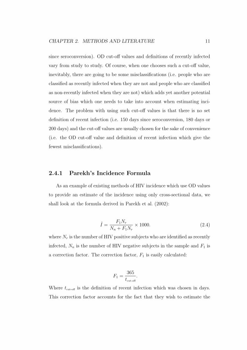
2.4.1 Parekh’s Incidence Formula
As an example of existing methods of HIV incidence which use OD values
to provide an estimate of the incidence using only cross-sectional data, we
shall look at the formula derived in Parekh et al. (2002):
I =F1Nr
Nn + F1Nr
× 1000. (2.4)
whereNr is the number of HIV positive subjects who are identified as recently
infected, Nn is the number of HIV negative subjects in the sample and F1 is
a correction factor. The correction factor, F1 is easily calculated:
F1 =365
tcut-off.
Where tcut-off is the definition of recent infection which was chosen in days.
This correction factor accounts for the fact that they wish to estimate the

CHAPTER 2. METHODS AND LITERATURE 12
incidence for a year but have only included HIV positive subjects who sero-
converted tcut-off days before their first positive HIV test.
One of the main benefits claimed for this method of incidence estimation
is that we do not need the results of HIV tests at 2 different time points
for every subject. Instead, we need only the results from one HIV test and
then use the OD value of those who are HIV positive to estimate how many
seroconverted within the last year.
An improved version of the formula is offered in the same paper (Parekh
et al. (2002)) which adds a second correction factor, F2 which adjusts for
misclassification of which infections are recent. This second correction factor
is calculated as follows:
F2 =Pobs + (spec)− 1
Pobs[(sens) + (spec)− 1]. (2.5)
The improved version of the formula from Parekh et al. (2002) is then
I =F1F2Nr
Nn + F1F2Nr
× 1000. (2.6)
Here Pobs is the proportion of HIV positive subjects who tested as recently
infected, (spec) is the specificity (i.e. the proportion of non-recent infections
which were classified as non-recent) and (sens) is the sensitivity (i.e. the pro-
portion of recent infections which were classified as recent). Figure 2.1 below
helps to demonstrate how this correction factor adjusts for misclassifications.

CHAPTER 2. METHODS AND LITERATURE 13
Figure 2.1: Flow Diagram of Recency Classification
Figure 2.1 shows the probabilities of being classified as recently infected
or not based on whether the individual is truly recently infected or not and
allows us to deduce the following (where θ is the incidence estimate):
Pobs = θ(sens) + (1− θ)(1− (spec))
= θ(sens) + 1− (spec)− θ + θ(spec)
= θ[(sens) + (spec)− 1] + 1− (spec).
By rearranging this equation, we get
θ =Pobs + (spec)− 1
(sens) + (spec)− 1.
Then F2 is simply
F2 =θ
Pobs
=Pobs + (spec)− 1
Pobs[(sens) + (spec)− 1], (2.7)

CHAPTER 2. METHODS AND LITERATURE 14
as in equation 2.5.
One problem with this correction factor is that the specificity and sensi-
tivity are difficult to estimate and will depend on the OD cut-off value which
is chosen and also the definition of recent infection (although this is high-
lighted in the paper).
A problem with both of Parekh’s formulae is that they do not take into
account the fact that the incidence rate may not be constant across the year.
They only include HIV positive subjects who seroconverted within 160 days
of their HIV test and assume that the incidence rate for the first 160 days is
the same as that for the whole year. This approach to incidence calculation
also fails to take missing data into account, i.e. people who are asked to take
part in the study but refuse, which (assuming there was any) may contribute
towards a biased estimate of HIV incidence. For example, people who refuse
to partake in the study may be more likely to contract HIV than those who
do not.
2.4.2 McDougal’s Incidence Formula
Another example of a formula which is used in cross-sectional HIV testing
is that derived in McDougal et al. (2006) which is given as
IMcD =fNr
fNr + ωNn
× 1000. (2.8)
Where ω is the mean period of time (in years) from seroconversion to
reaching an OD value equal to the recency cut-off value and f is a correction
factor calculated as
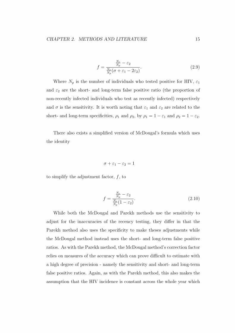
CHAPTER 2. METHODS AND LITERATURE 15
f =
Nr
Np− ε2
Nr
Np(σ + ε1 − 2ε2)
. (2.9)
Where Np is the number of individuals who tested positive for HIV, ε1
and ε2 are the short- and long-term false positive ratio (the proportion of
non-recently infected individuals who test as recently infected) respectively
and σ is the sensitivity. It is worth noting that ε1 and ε2 are related to the
short- and long-term specificities, ρ1 and ρ2, by ρ1 = 1− ε1 and ρ2 = 1− ε2.
There also exists a simplified version of McDougal’s formula which uses
the identity
σ + ε1 − ε2 = 1
to simplify the adjustment factor, f , to
f =
Nr
Np− ε2
Nr
Np(1− ε2)
. (2.10)
While both the McDougal and Parekh methods use the sensitivity to
adjust for the inaccuracies of the recency testing, they differ in that the
Parekh method also uses the specificity to make theses adjustments while
the McDougal method instead uses the short- and long-term false positive
ratios. As with the Parekh method, the McDougal method’s correction factor
relies on measures of the accuracy which can prove difficult to estimate with
a high degree of precision - namely the sensitivity and short- and long-term
false positive ratios. Again, as with the Parekh method, this also makes the
assumption that the HIV incidence is constant across the whole year which

CHAPTER 2. METHODS AND LITERATURE 16
may not be the case. The estimates which it produces will also depend on the
definition of recent infection chosen as well as the corresponding OD cut-off
value.
2.5 Missing Data Mechanisms
When dealing with missing data, we must consider the mechanisms which
cause the data to be missing in the first place. Three such mechanisms are
described in Little & Rubin (2002) and are detailed below
Suppose we have a data matrix Y = (yij) with no missing values which
has I rows and J columns where yij is the value of the variable Yj for the ith
subject. Then, for missing data, we create a missing data indicator matrix,
M , also with I rows and J columns, with entries mij = 1 if yij is missing
and mij = 0 if yij is present. The conditional distribution, f(M |Y, ϕ), where
ϕ represents unknown parameters, describes the missing data mechanism.
A missing data mechanism is called missing completely at random (MCAR)
if missingness does not depend on the values in the data set (whether missing
or not), i.e.
f(M |Y, ϕ) = f(M |ϕ),∀Y, ϕ.
A missing data mechanism is called missing at random (MAR) if miss-
ingness depends only on the values in the data set which are observed and
not on the values which are missing, i.e. (assuming the previously described
data set)

CHAPTER 2. METHODS AND LITERATURE 17
f(M |Y, ϕ) = f(M |YOBS, ϕ),∀YMISS, ϕ.
Where YOBS denotes values of Y which are not missing and YMISS denotes
values of Y which are missing.
If the distribution of M does depend on the missing values of Y (i.e. on
YMISS), then the missing data mechanism is called not missing at random
(NMAR)
2.6 Missing Data Imputation
If the missing data mechanism is MCAR, then the values which are miss-
ing do not differ systematically from those which are observed. As such,
the missing data do not introduce any bias when performing a complete-case
analysis and imputation of the missing values is not necessary. However,
if the missing data mechanism is not MCAR but MAR then imputation of
missing values becomes important.
In some instances, missing data values can be imputed deterministically,
that is, the missing values can be determined from non-missing values ob-
served on the same individual depending, of course, on prior knowledge about
the variable for which data values are missing. For example, with HIV test-
ing, once someone has been diagnosed as HIV-positive they cannot go back
to being HIV-negative. As such, once they have tested positive for HIV, all
following HIV tests can be imputed as positive. Similarly, if someone tests
negative for HIV, then all previous tests can be imputed as negative. Of

CHAPTER 2. METHODS AND LITERATURE 18
course, deterministic imputation such as this requires the assumption that
all tests are accurate.
Where missing values are present, there are several methods for filling-in,
or imputing, these values. These methods of imputation generally take two
forms which are described in Little & Rubin (2002) as being explicit or im-
plicit modelling. Explicit modelling is where the predictive distribution used
for imputing the missing values (which is based on the observed values in the
data) is that of a formal statistical model which means that the associated
assumptions are explicit. An example of explicit modelling is where missing
values are imputed using a regression model with the missing value as the
response variable and observed values of the unit with missing data as the
explanatory variable. Implicit modelling is where the predictive distribution
is based on an algorithm which implies an underlying distribution and hence
the underlying assumptions are implicit. An example of implicit modelling
is where one imputes the missing value by drawing from a sample of non-
missing values taken from units which are classified as similar according to
the observed values of the unit for which data is missing.
2.7 Confidence Intervals using Imputed Data
Sets
Once complete data sets have been created using the imputation methods
described in the previous section, we can use each set of data to produce a
point estimate of the same parameter (e.g. incidence rate) and combine
these to obtain a confidence interval. This can be done as described in Little

CHAPTER 2. METHODS AND LITERATURE 19
& Rubin (2002). Supposing we have D imputed data sets which are each
divided into H strata, the estimate of the HIV incidence from the dth data
set, θd, is given by
θd =H∑
h=1
nh
nθh(d).
Where nh is the number of subjects in the hth strata, n is the total
number of subjects in the sample and θh(d) is the estimated incidence in the
hth stratum of the dth data set. The variance associated with the estimated
incidence in each data set is given by
var(θd) =H∑
h=1
(nh
n
)2
×s2h(d)nh
.
Where s2h(d) is the estimated variance of the incidence estimate in the hth
strata of the dth data set.
With D estimates of the incidence and associated variance, we can now
proceed to calculate an overall estimate for the D imputed data sets. The
average incidence estimate of theD imputed data sets, θT is simply calculated
as
θT =1
D
D∑d=1
θd.
The total variability associated with θT is then given by
VT =1
D
D∑d=1
var(θd) +D + 1
D
1
D − 1
D∑d=1
(θd − θT )2.

CHAPTER 2. METHODS AND LITERATURE 20
Now, θ − θ has approximately a t distribution with centre zero, squared
scale VT and degrees of freedom given by
d.f. = (D − 1)
1 +1
D + 1
1D
D∑d=1
var(θd)
1D−1
D∑d=1
(θd − θT )2
2
.
We now have all the appropriate information to create an approximate
95% confidence interval for θ. This is given by:
θT ± t0.025,d.f.
√VT
d.f.+ 1.
2.8 Data Simulation
In order to test different methods of incidence estimation one can simu-
late various datasets for which we choose the ‘true’ values of the population
parameters which we are trying to estimate (i.e. the HIV incidence). In doing
so, we can compare our estimates of the HIV incidence to that value of the
incidence which was chosen prior to the simulation and gain an impression
of how well they perform.
2.8.1 Bias
Once the data sets have been simulated, we need some means of quantify-
ing the difference between our estimate of a parameter and the true parameter
value. One way of doing this is to calculate the bias of our estimator, this
is simply the difference between the expected value of the estimator and the
actual value of the parameter which it estimates. The bias is

CHAPTER 2. METHODS AND LITERATURE 21
Bias(θ) = E(θ)− θ
which is estimated by
1
n
n∑i=1
θi − θ. (2.11)
Here θ is our estimate of the parameter value, θ, n is the number of
simulated data sets and θi is the value of our estimate in the ith data set.
2.8.2 Root Mean Squared Error
Another means of quantifying the difference between our estimator and
the associated parameter is to calculate the root mean squared error (RMSE).
This is the square root of the mean square error (MSE) which is the mean of
the squares of the differences between our estimator values and the parameter
value. The root mean squared error is
RMSE(θ) =
√MSE(θ)
=
√E[(θ − θ)2]
which is estimated as
√√√√ 1
n
n∑i=1
(θi − θ)2. (2.12)

CHAPTER 2. METHODS AND LITERATURE 22
2.9 Our intended approach to HIV incidence
estimation
Given the reasonably large number of missing values in the dataset, it
seems likely that some method for imputing these missing values would be
useful when producing estimates of the incidence of HIV. We will attempt to
use multiple imputation of missing values along with the Parekh and McDou-
gal approaches to estimating HIV incidence to obtain improved estimates.

Chapter 3
Preliminary Analysis
3.1 Missing Data
One of the most obvious problems with our data set is that there is a lot
of missing values, particularly with HIV test results. There are a number of
reasons why these missing values may have occurred. Some of the individuals
refused to have the test taken, while others moved away from the area and
were lost to follow up. Other missing values are the result of inconclusive
HIV tests.
Table 3.1 below shows the number and proportion of missing values for
some of the variables in our data. The total population size was 20,284. The
7 individuals for whom we have no age are the same 7 for whom we have no
information about sex. In fact, in the cases of these 7 individuals, we have
no information whatsoever and, as such, it was decided that these subjects
should be removed from the data set completely. It would also appear from
this table that the number of visits which were completed reached a peak
at the second stage of testing given that this is the stage with the lowest
23

CHAPTER 3. PRELIMINARY ANALYSIS 24
number of missing visit dates. Reassuringly, only a small number of the tests
of recent infection are missing at stage 2 (0.56%), however, the relatively large
number of missing recency test results at stage 3 (46%) is rather worrying.
The recency test was not carried out at the first stage of testing.
Table 3.1: Number of missing values for variables in data
Age 7 (0.034%)
Sex 7 (0.034%)
Date of Visit 1 5580 (26.954%)
Date of Visit 2 3137 (15.153%)
Date of Visit 3 6615 (31.953%)
Recency test 1 N/A N/A
Recency test 2 16 (0.559%)
Recency test 3 794 (45.949%)
For the purpose of our analysis, we have chosen to include only those
individuals who were either female and aged 15 to 49 years or male and aged
15 to 54 years, in accordance with the design of the cohort study from which
the data is taken. A person’s age is taken to be their age on the day on
which they entered the study. Furthermore, we have included only those
individuals who were resident in the surveillance area on the day on which
they entered the study in our analysis.
Table 3.2 below shows the patterns of results of HIV tests at the three
stages. In this table, N is a negative HIV test, P is a positive HIV test and
X is a missing value. The subscripts on the numbers of HIV-positive people
are the number who are classified as recently infected, according to their OD

CHAPTER 3. PRELIMINARY ANALYSIS 25
value. From this table, we can see that the number of missing values for HIV
tests is quite high at every stage. It is also worth noting that the proportions
of HIV positive people who go on to have a missing value for their next HIV
test are always higher than the proportions of HIV negative people who go
on to have a missing value for their next test. This would suggest that the
missing data mechanism is unlikely to be MCAR. Also highlighted by this
table is the fact that this HIV test is not 100% accurate as demonstrated by
the fact that a very small proportion of the tests results go from positive at
one stage to negative at the next.

CHAPTER 3. PRELIMINARY ANALYSIS 26
Table 3.2: Table of HIV Status by HIV Status at Previous Stage
Stage 1 Stage 2 Stage 3
N 1945 (50.0%)
N 3888 (41.7%) P 542 (1.4%)
X 1889 (48.6%)
N 1 (0.6%)
N 9317 (49.1%) P 17345 (1.9%) P 650 (37.6%)
X 107 (61.8%)
N 898 (17.1%)
X 5256 (56.4%) P 722 (1.4%)
X 4286 (81.5%)
N 2 (50%)
N 4 (0.2%) P 00 (0%)
X 2 (50%)
N 1 (0.1%)
P 2606 (13.7%) P 79721 (30.6%) P 3281 (41.2%)
X 468 (58.7%)
N 2 (0.1%)
X 1805 (69.3%) P 2440 (13.5%)
X 1559 (86.4%)
N 1454 (43.3%)
N 3356 (47.6%) P 436 (1.3%)
X 1859 (55.4%)
N 3 (0.3%)
X 7045 (37.1%) P 87448 (12.4%) P 2721 (31.1%)
X 599 (68.5%)
N 2231 (79.3%)
X 2815 (40.0%) P 5476 (19.4%)
X 37 (1.3%)
The subscript on a number of positive tests denotes the number of those individuals classified as recently infected.
CHAPTER 3. PRELIMINARY ANALYSIS 27
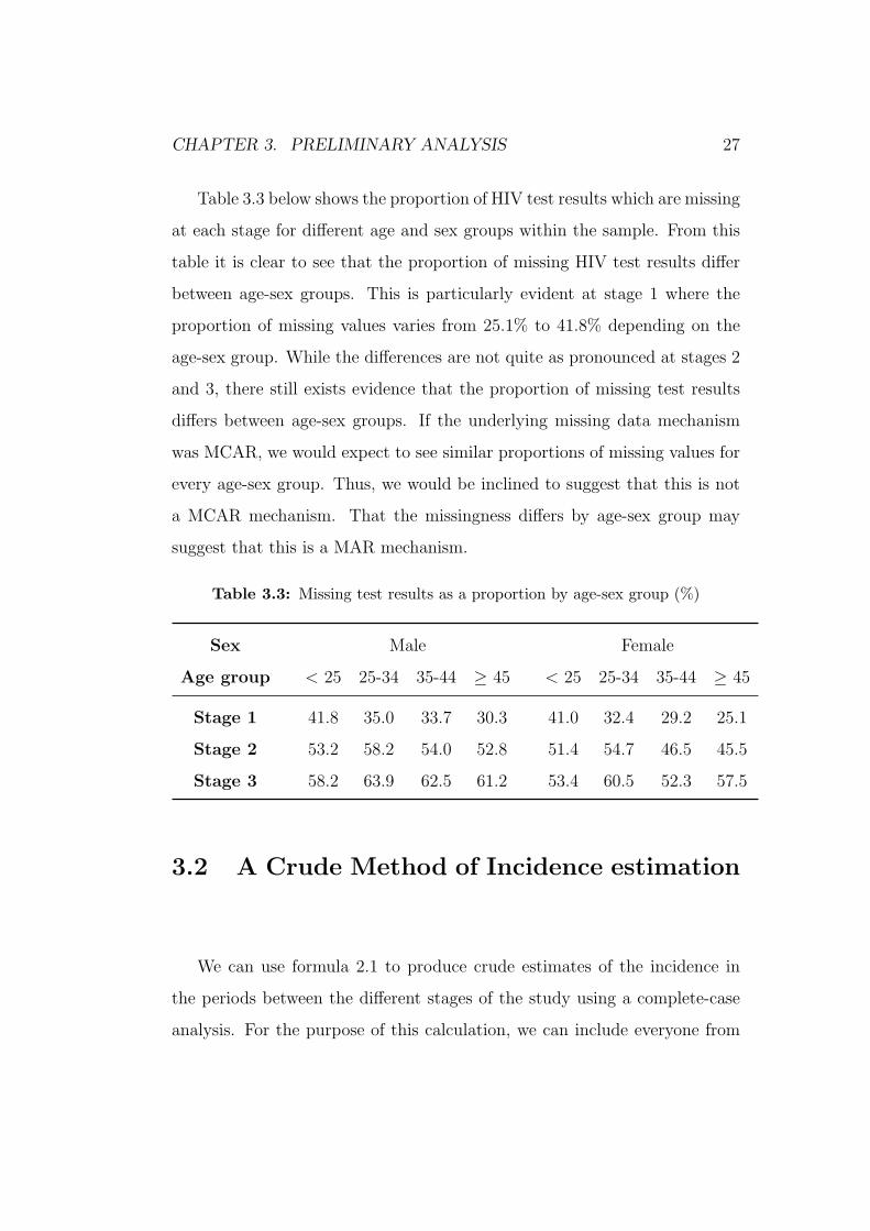
Table 3.3 below shows the proportion of HIV test results which are missing
at each stage for different age and sex groups within the sample. From this
table it is clear to see that the proportion of missing HIV test results differ
between age-sex groups. This is particularly evident at stage 1 where the
proportion of missing values varies from 25.1% to 41.8% depending on the
age-sex group. While the differences are not quite as pronounced at stages 2
and 3, there still exists evidence that the proportion of missing test results
differs between age-sex groups. If the underlying missing data mechanism
was MCAR, we would expect to see similar proportions of missing values for
every age-sex group. Thus, we would be inclined to suggest that this is not
a MCAR mechanism. That the missingness differs by age-sex group may
suggest that this is a MAR mechanism.
Table 3.3: Missing test results as a proportion by age-sex group (%)
Sex Male Female
Age group < 25 25-34 35-44 ≥ 45 < 25 25-34 35-44 ≥ 45
Stage 1 41.8 35.0 33.7 30.3 41.0 32.4 29.2 25.1
Stage 2 53.2 58.2 54.0 52.8 51.4 54.7 46.5 45.5
Stage 3 58.2 63.9 62.5 61.2 53.4 60.5 52.3 57.5
3.2 A Crude Method of Incidence estimation
We can use formula 2.1 to produce crude estimates of the incidence in
the periods between the different stages of the study using a complete-case
analysis. For the purpose of this calculation, we can include everyone from

CHAPTER 3. PRELIMINARY ANALYSIS 28
our data who had at least two HIV tests, the first of which was negative.
We know that each subject’s tests were supposed to be taken approximately
a year apart from one another in this study so if we assume that the HIV
tests are exactly a year apart we can produce the incidence estimates shown
in table 3.4 below.
Looking at table 3.4, we can see that the incidence rate between stage 1
and 2 is estimated as 42.6 infections per 1000 person years. In other words we
would estimate that, between stages 1 and 2, 42.6 of every 1000 HIV-negative
people in the at-risk population would become HIV-positive within a year.
Similarly, using this method we would estimate that, between stages 2 and
3, 27.7 of every 1000 HIV-negative people in the at-risk population would
become HIV-positive within a year. If we look instead at the first and final
stage of this study, then we would estimate that, between stages 1 and 3, 62.9
of every 1000 HIV-negative people in the at-risk population would become
HIV-positive within the two-year period, an average incidence rate across
time of 31.5 infections per 1000 person years. This is not consistent with
the calculations for the two time periods separately, which give a combined
estimate of
1
2
{42.6
1000+
27.7
1000×(1− 42.6
1000
)}= 34.6 per 1000 person years.

CHAPTER 3. PRELIMINARY ANALYSIS 29
Table 3.4: Crude Incidence Estimates for Different Stages of the Study
Incidence
Stages (No. Infections per 1000 person years)
1 → 2 42.60
2 → 3 27.73
1 → 3 31.47
However, these estimates are based on the assumption that there is ex-
actly a year between each HIV test. Looking at figure 3.1 below, however,
we can see that this is clearly not the case.
Figure 3.1 shows the histograms of time between HIV tests for different
stages of the study with a line indicating what the time should be if there
was exactly a year between each test. Looking first at the histogram of time
between the HIV tests at stage 1 and 2, we can clearly see that the majority
of subjects waited for more than a year after their first HIV test to receive
their second HIV test, with some subjects waiting over 800 days. This would
certainly seem to cast some doubt on the accuracy of our estimation of the
incidence between stage 1 and stage 2 in table 3.4. Looking now at the his-
togram of time between subjects’ HIV tests at stage 2 and stage 3, we can
see that the average time between these tests is actually reasonably close
to being a year. As such, our estimate of the incidence between stages 2
and 3 in table 3.4, while still far from perfect, may well be a more accurate
reflection of the actual incidence than our estimate for stages 1 and 2. It is
also clear from the histogram of time between subjects’ HIV tests at stages
1 and 3 that the average time between the first and last HIV test is greater
than 2 years since the majority of the times lie to the right of the line at 2

CHAPTER 3. PRELIMINARY ANALYSIS 30
years. This is to be expected since many of the times used for this plot will
be the sum of the time between tests at stages 1 and 2 and the time between
tests at stages 2 and 3. This would lead us to believe that our estimate of
the incidence between stage 1 and 3 is not very accurate.

CHAPTER 3. PRELIMINARY ANALYSIS 31
Histogram of Time between Test at Stage 1 and Test at Stage 2
Time (Days)
Fre
quen
cy
0 200 400 600 800 1000 1200
010
0020
00
Histogram of Time between Test at Stage 2 and Test at Stage 3
Time (Days)
Fre
quen
cy
0 200 400 600 800 1000 1200
010
0020
00
Histogram of Time between Test at Stage 1 and Test at Stage 3
Time (Days)
Fre
quen
cy
0 200 400 600 800 1000 1200
010
0020
00
Figure 3.1: Histograms of Time between HIV Tests at different Stages

CHAPTER 3. PRELIMINARY ANALYSIS 32
3.3 Taking time into account when estimat-
ing incidence
In order to improve our estimate, we must take the time between HIV
tests into account when calculating the incidence. We can do so using for-
mula 2.3 where the tis are the times between HIV tests for those who didn’t
seroconvert and the time to seroconversion for those who did. To begin with,
the time of seroconversion is estimated as the midpoint between the subject’s
last negative HIV test and their first positive HIV test. Using this formula
we can produce the results in table 3.5 below.
Table 3.5 shows the estimates of incidence between different stages which
are produced by using formula 2.3. From this table we can see that the
incidence estimates produced using formula 2.3 are lower than those which
did not take time between HIV test into account (using formula 2.2). The
incidence between stage 1 and stage 2 is certainly much lower than that in
table 3.4 and so we would now estimate that 32.9 of every 1000 HIV-negative
subjects in the at-risk population would become HIV-positive within a year.
This is still slightly higher than our estimates of the incidence between stages
1 and 2 and between stages 1 and 3. The stage 1 → 3 incidence estimate is
still not consistent with the other estimates.

CHAPTER 3. PRELIMINARY ANALYSIS 33
Table 3.5: Incidence Estimates for Different Stages of the Study using time be-
tween HIV Tests
Incidence
Stages (No. Infections per 1000 person years)
1 → 2 32.93
2 → 3 28.62
1 → 3 28.57
While taking time into account has helped improve our incidence esti-
mates slightly, there are obviously many more improvements which can be
made.
3.4 Applying the Formula Derived in Parekh
et al. (2002) to our Data
3.4.1 Applying Parekh’s formula to the same data used
in sections 3.2 and 3.3
In order to apply the formula for calculating incidence derived in Parekh
et al. (2002) shown in equation 2.6, we must first calculate the individual
terms of the equation. We shall first calculate the incidence between the
first and second stage of data collection by including all subjects who were
negative at the first stage and then either negative or positive at the second
stage. Initially, we will use the same data which was used in sections 3.2 and
3.3 so as to enable comparisons between our crude methods and Parekh’s

CHAPTER 3. PRELIMINARY ANALYSIS 34
formula. However, we are able only to include those HIV positive subjects
for whom we have information about their OD value.
We shall begin by calculating the simplest part of the equation, the cor-
rection factor F1, which does not depend on our data and is simply calculated
as
F1 =365
153= 2.386.
Note that we are using the value of 153 as this is the number of days after
HIV infection for which someone is classified as recently infected according
to the article by Barnighausen et al. (2008) which used the same data set as
was available to us.
Now, to calculate the proportion of HIV positive subjects who tested as
recently infected (i.e. with an OD value of less than or equal to 0.8 - the cut-
off used in Barnighausen et al. (2008)) at the second stage of data collection,
Pobs, allowing for missing information about recency.
Pobs =No. Individuals who tested as recently infected at 2nd stage
Total No. HIV positive individuals at 2nd Stage
=45
173= 0.260.
It is also necessary to estimate the specificity (the proportion of non-
recent infections who tested as non-recent) and the sensitivity (the propor-
tion of recent infections who tested as recent). For the purpose of these
calculations, for those who tested negative for HIV at the first stage and
positive at the second stage, we shall take their date of seroconversion as the
midpoint between the dates of their first and second HIV tests

CHAPTER 3. PRELIMINARY ANALYSIS 35
Specificity =Total No. of non-recent who tested as non-recent
Total No. of non-recently infected
=117
161= 0.727 = 72.7%
and
Sensitivity =Total No. of recently infected who tested as recently infected
Total No. of recently infected
=1
7= 0.143 = 14.3%.
Clearly, these values for sensitivity and specificity are quite low, par-
ticularly the 14.3% sensitivity. This is likely a result of the fact that the
time between HIV testing at the first stage and the second stage was ap-
proximately a year for each individual meaning that few of the HIV positive
individuals would have registered as recently infected (within 153 days in
this case). As a result, we have instead chosen to use the sensitivity and
specificity values which were provided in the paper Parekh et al. (2002) as
these were calculated using a sample of individuals who were tested for HIV
much more frequently. These values are
Sensitivity = 82.7%
Specificity = 97.8%.
So, we are now able to calculate F2 as follows:

CHAPTER 3. PRELIMINARY ANALYSIS 36
F2 =Pobs + (spec)− 1
Pobs[(sens) + (spec)− 1]
=0.268 + 0.978− 1
0.268× (0.827 + 0.978− 1)
=0.246
0.216
= 1.140.
All we need now in order to be able to calculate our estimate of the
HIV incidence is the number of HIV positive subjects who tested as recently
infected, Nr, and the number of HIV negative subjects in the sample, Nn.
At stage 2, these are:
Nr = 45
Nn = 3888.
So, our estimate of the HIV incidence in one year is
I =F1F2Nr
Nn + F1F2Nr
× 1000
=2.386× 1.137× 45
3888 + 2.386× 1.137× 45× 1000
=122.08
4010.08× 1000
= 30.52 infections per 1000 person years.
That is, we would estimate that approximately 30 of every 1000 HIV-negative
subjects in the at-risk population would become infected within a year.
If we now apply equation 2.6 to the data between the other stages, then
we get the results shown in table 3.6 below.

CHAPTER 3. PRELIMINARY ANALYSIS 37
Table 3.6: Incidence Estimates for Different Stages of the Study using Parekh’s
Final Method
Incidence
Stages (No. Infections per 1000 person years)
1 → 2 30.52
2 → 3 5.96
1 → 3 2.10
From table 3.6, we can see that the estimates for the incidence between
stages 2 and 3 and between stages 1 and 3 using Parekh’s method are much
lower than that for the incidence between stages 1 and 2 and certainly lower
than the incidence estimates using the other methods. This is likely a result
of the fact that only 4 of the HIV positive specimens at stage 3 were classified
as recently infected according to the OD value compared to 45 classified as
recently infected at stage 2.
Table 3.6 shows the results of using one form of Parekh’s formula for
estimating incidence. There is another, simpler form (shown in equation
2.4) which is similar but does not include the second correction factor which
adjusts for misclassifications in the recency test. It would certainly be worth-
while estimating the incidence using this simpler form to see how the results
compare. Upon doing so, one gains the results shown in table 3.7 below.

CHAPTER 3. PRELIMINARY ANALYSIS 38
Table 3.7: Incidence Estimates for Different Stages of the Study using Parekh’s
intermediate Method
Incidence
Stages (No. Infections per 1000 person years)
1 → 2 26.87
2 → 3 5.58
1 → 3 3.34
Looking at table 3.7 (and table 3.6), we can see that there is very little
difference in the estimate of the incidence from stage 2 to stage 3 between be-
tween the two forms of Parekh’s formula. However, the estimate from stages
1 to 2 is slightly lower while the estimate from stages 2 to 3 is slightly higher.
So, it would appear that correcting for the misclassification in recency testing
does, indeed, make some difference to the final estimate of the incidence and
so it would seem wise to use the more complicated form of Parekh’s formula
since misclassification is almost inevitable.
3.4.2 Applying Parekh’s formula to an expanded dataset
Unlike with our crude estimates of incidence (sections 3.2 & 3.3), Parekh’s
formula does not require the results from two HIV tests taken at separate
times. Instead, it requires only the results of one HIV test and the OD
values of those who tested as HIV positive at that time to classify HIV
positive specimens as recently infected or not. As such, we can expand the
amount of data used in the calculation of our incidence estimates to include
those people who had just one HIV test (although, for our calculations of the

CHAPTER 3. PRELIMINARY ANALYSIS 39
incidence at each stage we will be excluding anyone who has previously tested
positive). So, rather than estimates of the incidence between stages, we now
have estimates of the incidence at each stage. These are shown in table 3.8
below (using both the intermediate and final forms of Parekh’s method)
Table 3.8: Incidence Estimates for expanded dataset using Parekh’s Methods
Incidence (No. Infections per 1000 person years)
Stage Intermediate Method Final Method
2 29.72 27.92
3 5.81 3.31
From the results in table 3.8, we can see that these estimates of the
HIV incidence are generally slightly higher than those based on the smaller
dataset. Unfortunately, incidence estimates for stage 1 were not possible as
we have no OD values for the HIV-positive specimens at this stage. It is
also worth noting the small values for the incidence at stage 3. It appears to
have come about as a results of a low proportion of HIV-positive specimens
being classified as recently infected at stage 3. Clearly, this is one weakness
of Parekh’s formula. That is, that it requires reasonably large proportions of
the HIV-positive specimens to be classified as recently infected.
3.4.3 Applying McDougal’s methods of incidence esti-
mation to our data
In chapter 2, we looked at several formulae for estimating HIV incidence.
These include the formulae derived by McDougal (section 2.4.2). Table 3.9

CHAPTER 3. PRELIMINARY ANALYSIS 40
below shows the results of applying these formulae to our data for stages 2
and 3 of the study.
Table 3.9: Table of HIV incidence estimates at different stages using different
McDougal formulae
HIV incidence
Method (Infections per 1000 person years)
Stage 2 Stage 3
McDougal 24.01 3.36
McDougal (Simplified) 24.68 3.46
From table 3.9, we can see that the estimates of HIV incidence at stage
2 produced by each method are reasonably similar with estimates of 24.01
and 24.68 infections per 1000 person years. Likewise, the estimates of HIV
incidence at stage 3 are also rather similar at 3.36 and 3.46 infections per
1000 person years. However, the methods shown here seem to suffer from
the same problem as occurred with Parekh’s method, that is, low numbers
of HIV positive specimens registering as recently infected (according to the
OD value) at stage 3 leading to very low estimates of HIV incidence. We
can only speculate as to how this problem has arisen. Potentially, there is a
major problem with OD or a serious sampling bias at stage 3.

Chapter 4
Imputation of Missing Values
4.1 Missing Values in our Data Set
We produced a number of different estimates of the HIV incidence in chap-
ter 3. However none of these incidence estimates took the missing values in
our data into account meaning that there may well exist some response bias
which we have not yet taken into account. In order to try and improve our es-
timates, it was decided to find a method of imputing the missing data values.
When an HIV test result is missing, two distinct pieces of information
must be imputed: HIV status(either HIV positive or negative) and time
between tests (to be used in some estimation procedures). We start by de-
scribing the deterministic imputation of HIV status.
4.2 Deterministic Imputation of HIV Status
Presently, there is no cure for HIV. As such, once someone has serocon-
verted they cannot return to being HIV-negative. Assuming that the HIV
41

CHAPTER 4. IMPUTATION OF MISSING VALUES 42
results for which we do have information are correct, we are then able to im-
pute some of the HIV results deterministically. That is, if an individual tests
as HIV-negative at one stage, then they must be HIV-negative at all preced-
ing stages. Similarly, if an individual tests as HIV-positive at one stage then
they must be HIV-positive at all following stages. In the very small num-
ber of cases where an individual tests as HIV-positive at one stage and then
HIV-negative at a later stage, it was decided to back-fill the HIV-negative
result rather than forward-fill the HIV-positive results. If we apply this to
our data, we produce the HIV test result sequences shown in table 4.1 below.
Looking at table 4.1, we can see that, after our deterministic imputation,
once someone tests positive for HIV, they remain HIV-positive for the re-
mainder of the study. Also, an individual who has a missing HIV test result
at one stage can only be classified as positive or missing at any following
stages since, if they were to be negative at a later stage, then the missing
value would have been reclassified as a negative HIV test result. Comparing
this to our table of the original data (table 3.2), we can see that there is a
large increase in the number of subjects classified as HIV-negative at stage
1 with 9317 individuals classified as HIV-negative in our original data and
14914 classified as HIV-negative after deterministic imputation. There is ac-
tually a small decrease in the number of the HIV-positive subjects at stage
1 from the original data to our data after deterministic imputation. This
is the result of the fact that we decided to back-fill the negative results for
those individuals who went from positive to negative and the fact that we
are forward-filling positive results so we can’t impute any positive values at
stage 1.

CHAPTER 4. IMPUTATION OF MISSING VALUES 43
Table 4.1: Table of HIV Status by HIV Status at Previous Stage
Stage 1 Stage 2 Stage 3
N 14914 (78.6%)
N 6537 (63.0%)
N 10384 (69.6%) P 97 (0.9%)
X 3750 (36.1%)
P 172 (1.2%) P 172 (100%)
X 4358 (29.2%)P 72 (1.7%)
X 4286 (98.3%)
P 2599 (13.7%) P 2599 (100%) P 2599 (100%)
P 871 (59.9%) P 871 (100%)
X 1455 (7.7%)X 584 (40.1%)
P 547 (93.7%)
X 37 (6.3%)
If we use the data set produced by this deterministic imputation, then
we can produce the crude HIV incidence estimates shown in table 4.2 below.
Note that these incidence estimates use the method shown in equation 2.1
which does not take time between tests into account. This is because many
of the visit dates are also missing, leaving us unable to ascertain the time
between visits.
Comparing table 4.2 to table 3.4, it is clear that the incidence estimates
for the data produced using deterministic imputation are much lower than
those from the original data. The reason for this is that there is a much
greater number of negative HIV test results in the data which can be back-

CHAPTER 4. IMPUTATION OF MISSING VALUES 44
filled using deterministic imputation than there is positive test results which
can be forward-filled. The fact that an individual has to be HIV-negative
at the earlier stage to be included in incidence estimates also means that
all the deterministically imputed negative results can be incorporated into
our incidence estimates whereas only a small fraction of the imputed positive
results can be used in incidence estimates. The only imputed positive results
which can be included in our estimates are the 107 individuals who had an
HIV test result sequence of N P X in our original data. These individuals
would then be imputed as N P P which would contribute towards the estimate
of the incidence between stages 1 and 3 since they are negative at stage 1
and newly classified as positive at stage 3.
Table 4.2: Crude HIV Incidence estimates before and after deterministic impu-
tation
Incidence(per 1000 person years)
Stages Before After
1 → 2 42.60 16.29
2 → 3 27.73 14.62
1 → 3 31.47 24.79
Table 4.3 below contains the proportion of missing values by age and
sex group after deterministic imputation. At each stage, there is noticeable
variability in the proportion of missing values between age-sex groups. This
is particularly evident at stages 1 and 3 where the difference between the
highest and lowest proportions is greater than 15%. With this in mind, it is
important that we take age and sex into account when we proceed to impute
the remaining missing test results probabilistically.
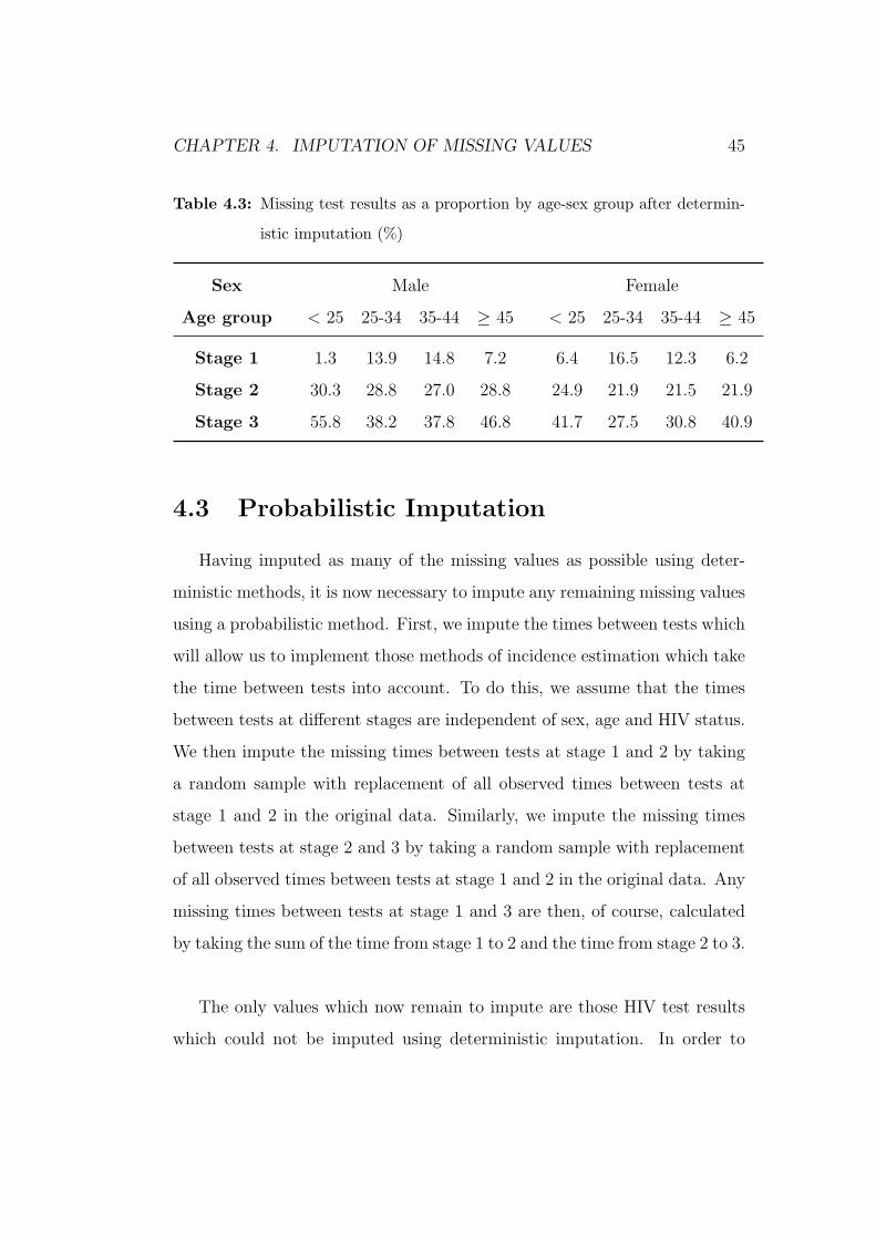
CHAPTER 4. IMPUTATION OF MISSING VALUES 45
Table 4.3: Missing test results as a proportion by age-sex group after determin-
istic imputation (%)
Sex Male Female
Age group < 25 25-34 35-44 ≥ 45 < 25 25-34 35-44 ≥ 45
Stage 1 1.3 13.9 14.8 7.2 6.4 16.5 12.3 6.2
Stage 2 30.3 28.8 27.0 28.8 24.9 21.9 21.5 21.9
Stage 3 55.8 38.2 37.8 46.8 41.7 27.5 30.8 40.9
4.3 Probabilistic Imputation
Having imputed as many of the missing values as possible using deter-
ministic methods, it is now necessary to impute any remaining missing values
using a probabilistic method. First, we impute the times between tests which
will allow us to implement those methods of incidence estimation which take
the time between tests into account. To do this, we assume that the times
between tests at different stages are independent of sex, age and HIV status.
We then impute the missing times between tests at stage 1 and 2 by taking
a random sample with replacement of all observed times between tests at
stage 1 and 2 in the original data. Similarly, we impute the missing times
between tests at stage 2 and 3 by taking a random sample with replacement
of all observed times between tests at stage 1 and 2 in the original data. Any
missing times between tests at stage 1 and 3 are then, of course, calculated
by taking the sum of the time from stage 1 to 2 and the time from stage 2 to 3.
The only values which now remain to impute are those HIV test results
which could not be imputed using deterministic imputation. In order to

CHAPTER 4. IMPUTATION OF MISSING VALUES 46
do this, we first make note of the fact that, after deterministic imputation,
there remains only six possible sequences of HIV test results which contain
missing values. These are those missing test results which are not preceded
by a positive test result nor followed by a negative test result. These are
detailed in table 4.4 below.
Table 4.4: Table of sequences of HIV status after deterministic imputation
HIV Status
Stage 1 Stage 2 Stage 3
N X
NX
P
X
P P
XX
P
X
Furthermore, using the logic that was detailed in our method of deter-
ministic imputation, there are also a limited amount of possible sequences of
HIV test results which each of these missing value sequences can actually be
imputed as. These are set out in table 4.5 below.
CHAPTER 4. IMPUTATION OF MISSING VALUES 47
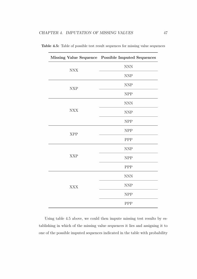
Table 4.5: Table of possible test result sequences for missing value sequences
Missing Value Sequence Possible Imputed Sequences
NNXNNN
NNP
NXPNNP
NPP
NXX
NNN
NNP
NPP
XPPNPP
PPP
XXP
NNP
NPP
PPP
XXX
NNN
NNP
NPP
PPP
Using table 4.5 above, we could then impute missing test results by es-
tablishing in which of the missing value sequences it lies and assigning it to
one of the possible imputed sequences indicated in the table with probability

CHAPTER 4. IMPUTATION OF MISSING VALUES 48
according to the ratio of these possible imputed sequences to one another in
the original data set.
For example, suppose we had missing values which lay in the sequence
NXX. This would then be assigned to be NNN, NNP or NPP. The probability
of being assigned to each of these can be calculated using the equations:
PNNN =nNNN
nNNN + nNNP + nNPP
PNNP =nNNP
nNNN + nNNP + nNPP
PNPP =nNPP
nNNN + nNNP + nNPP
Where PNNN, PNNP and PNPP are the probabilities of being assigned to be
NNN, NNP and NPP respectively and nNNN, nNNP and nNPP are the number of
times each sequence of test results appear in the original (pre-deterministic
imputation) sample. Where nijk = 0 in the sample, it is replaced by value 12
so as to eradicate the possibility of probabilities which are equal to zero.
Of course, we can extend this method of imputation to take into account
variations between different age and sex groups within the sample. This
is done by establishing the age-sex group to which the individual belongs
before calculating the probability with which they should be assigned to each
possible test result sequence using only those individuals (with fully observed
test result sequences) in the sample who belong to the same sub-group. That
is, for each imputation, we will define a set of age groups and every individual
will be assigned to an age-sex group according to, of course, their age and sex.

CHAPTER 4. IMPUTATION OF MISSING VALUES 49
Any individual with a missing test result after deterministic imputation will
have imputation probabilities calculated as detailed above using the observed
data within their assigned age-sex groups. We will carry out imputations
with between 1 and 6 age groups (and, therefore, between 2 and 12 age-sex
groups). The size of the age groups, of course, depend on the number of the
age groups. The age groups used in these imputations are detailed in 4.6
below.
Table 4.6: Table of age-group breakdowns by number of age-groups
No. age groups Breakdowns (years of age)
1 All ages
2 <35, ≥35
3 <28, 28-41, ≥42
4 <25, 25-34, 35-44, ≥45
5 <23, 24-30, 31-38, 39-47, ≥48
6 <21, 22-27, 28-32, 33-39, 40-47, ≥48
In order to allow us to take account of the variability in the results pro-
duced by this method of imputation, we will repeat this method of prob-
abilistic imputation ten times. Thus, rather than having a single imputed
dataset, we will have 10 imputed datasets. We will then be able to produce
10 estimates of the incidence (one from each of our imputed datasets) and
by taking the mean of these 10 estimates, we will thus be able to produce
an estimate of the incidence which should be more accurate than that which
would be produced with just one imputed dataset. Further to this, we will
also be able to produce 95% confidence intervals which take into account both
the variance associated with each of the 10 estimates (the within-imputation

CHAPTER 4. IMPUTATION OF MISSING VALUES 50
variance) and the variability between each of the imputations as described
in section 2.7.
Applying this imputation method to our dataset using four different age
groups (8 age-sex groups), we produce the estimates of the incidence detailed
in table 4.7 below. From this table, we can see that once this method has
been applied the mean estimates of the incidence are actually fairly con-
sistent with one another with the stage 1 to 2 incidence being reasonably
similar to that for stages 2 to 3 (31.04 and 30.92 infections per 1000 person
years respectively). This is quite reassuring in that we should be obtaining
reasonably similar results since we would not expect the incidence within the
cohort to change too much in the course of the few years across which the
testing took place. This may suggest that our method of imputation is ef-
fective since the stages 1 to 2 and stages 2 to 3 incidence were quite different
prior to imputation. Also reassuring is the fact that the estimated incidence
between stages 1 and 3 now lies between our estimates for the 1→2 and 2→3
incidence as we would expect.
Also from table 4.7, we can see that the variance associated with our es-
timates is larger for the 2 to 3 incidence than for the 1 to 2 incidence. This is
as expected since all those who went from HIV-negative to -positive between
stages 1 and 2 will be excluded for the 2 to 3 estimates because we use only
those who were negative at stage 2 to estimate the incidence between stages
2 and 3. Thus, the estimated incidence between stages 2 and 3 will be based
on smaller sample sizes, resulting in a larger variance.
From table 4.7, we also find justification for imputing multiple datasets.

CHAPTER 4. IMPUTATION OF MISSING VALUES 51
Clearly, there exists some variation in the the estimates of incidence which
each imputation produces and, as such, it is crucial that we impute the miss-
ing values more than once so that this variation can be incorporated into
our results such as with the 95% confidence intervals in the last row of this
table. That these confidence intervals are reasonably narrow means that we
are able to estimate the incidence with a fair degree of precision.

CHAPTER 4. IMPUTATION OF MISSING VALUES 52
Table
4.7:Incidence
estimates
from
multiple
imputationusing4agegroups(infectionsper
1000personyears)
1→2incidence
2→3incidence
1→3incidence
Imputation
Estim
ate
Variance
Estim
ate
Variance
Estim
ate
Variance
129.28
1.69
32.92
2.51
30.79
1.01
230.75
1.76
29.69
2.26
30.28
0.99
331.18
1.81
30.66
2.33
30.93
1.02
431.27
1.81
30.93
2.38
31.12
1.03
531.21
1.81
30.93
2.38
31.05
1.02
631.48
1.80
31.88
2.43
31.61
1.03
731.59
1.85
31.15
2.36
31.37
1.03
831.16
1.80
30.68
2.33
30.95
1.02
930.66
1.77
28.58
2.21
29.74
0.98
1031.81
1.87
31.79
2.45
31.77
1.06
MeanEst.(95%
C.I.)
31.04
(30.25,31.83)
30.92
(29.72,32.13)
30.96
(30.46,31.47)

CHAPTER 4. IMPUTATION OF MISSING VALUES 53
These results, in terms of variance and differences between imputations,
are similar to those which we achieved when imputing using different num-
bers of age groups. Tables A.1 to A.5 in appendix A contain the results for
multiple imputation using no age groups and using 2, 3, 5 and 6 age groups.
The mean incidences and associated 95% confidence intervals are shown in
table 4.8 below.
From table 4.8 below, we can see that the estimated incidence increases
with the number of age groups which were used in imputation. This is the
case until we get to around 4 age groups, beyond which the estimates either
decrease or increase only slightly. These differences suggest that the decision
to impute HIV test results within age-sex groups was correct. The changes
in our estimates level out around about 4 age groups which might imply
that this is the optimum number of age groups to use in our imputation of
this data. That the width of the confidence intervals do not differ greatly
between imputations with different numbers of age groups reassures us that
the accuracy of our estimates will not be greatly affected by the number of
age groups which we choose to carry out our imputations with.

CHAPTER 4. IMPUTATION OF MISSING VALUES 54
Table 4.8: Incidence estimates with 95% confidence intervals after multiple im-
putation (infections per 1000 person years)
Age Groups 1→2 2→3 1→3
1 27.75 (27.12, 28.38) 28.91 (27.72, 30.10) 28.23 (27.72, 28.73)
2 28.64 (27.70, 29.59) 29.63 (28.29, 30.98) 29.04 (28.51, 29.58)
3 29.46 (28.37, 30.55) 30.61 (29.35, 31.87) 29.93 (29.10, 30.75)
4 31.04 (30.25, 31.83) 30.92 (29.72, 32.13) 30.96 (30.46, 31.47)
5 31.47 (30.35, 32.58) 30.74 (29.82, 31.66) 31.15 (30.48, 31.82)
6 30.88 (30.00, 31.76) 30.39 (29.21, 31.58) 30.66 (30.15, 31.18)
Chapter 5
Data simulation
Having investigated various possible means for estimating the incidence
of HIV, it is important that we now find some means of assessing the relative
accuracy of the estimates which each produces. In order to do this, we are
going to simulate some new datasets. In doing so, we can apply our method
of estimating the HIV incidence to a dataset for which we know precisely the
values of the parameters which our method is designed to estimate. As such,
we are then able to compare our estimate of a parameter value to the true
value of that parameter.
Figure 5.1 below outlines the method which was used in our simulations.
This begins with the demography of the simulated population, once the de-
mographic parameters are set, they are not re-simulated. That is, through-
out the simulations, the individuals stay the same, it is only their test results
which are simulated again in the next simulation. After the demography
of the simulated population is set, the HIV test results and other relevant
information are simulated 1000 times. For each of these 1000 simulations,
we estimate the prevalence and incidence using various methods before em-
55

CHAPTER 5. DATA SIMULATION 56
ploying our imputation method to estimate the prevalence and incidence once
again. The numbers in figure 5.1 correspond to sections 1 to 6 of this chapter
for ease of reference, for example, ‘1.’ in the flow diagram corresponds to sec-
tion 5.1 (Simulating Demography) and ‘2.2’ in the flow diagram corresponds
to section 5.2.2.

CHAPTER 5. DATA SIMULATION 57
Figure 5.1: Flow Diagram of Simulation Method

CHAPTER 5. DATA SIMULATION 58
5.1 Simulating Demography
When simulating an appropriate dataset, there are a number of param-
eter values which must be set. The first of these parameters which we need
to consider is the size of the dataset which we wish to create. This can be
chosen more or less arbitrarily but we must bear in mind that the method of
imputation was designed using a reasonably large dataset. Unless otherwise
stated, all simulations presented here are carried out using a dataset con-
taining 20,000 individuals, which is approximately in line with the number
of records in our original dataset.
The next parameter values which must be decided upon are those per-
taining to age and sex. If we first take sex, then we must decide upon the
probability that each individual is male or female. Of course, the probabili-
ties that an individual is male (Pm) or female (Pf ) must sum to 1:
Pm + Pf = 1.
In our case, every simulation will be carried out with Pm = Pf = 0.5.
With the sex of each individual in the simulated population having been
established, we can now proceed to simulate the age of each individual. In
order to establish an age distribution which is consistent with that of the orig-
inal data, we simulate each age by taking a random draw with replacement
from the original population, dependent on sex. That is, if an individual is
simulated as female then their age is assigned by drawing at random (with
replacement) from the ages of all females in the original dataset. If an indi-
vidual is simulated as male then their age is assigned by drawing at random

CHAPTER 5. DATA SIMULATION 59
from the ages of all males in the original dataset. Once every individual in
the simulated dataset has an age and a sex, they can then be assigned to
groups depending on age and sex. This is important because, in our simu-
lated datasets, the incidence and prevalence will be allowed to vary between
different age-sex groups, as one would expect to see in reality.
5.2 Simulating HIV test results
5.2.1 Simulating time between tests
An important aspect in our calculation of HIV incidence is the length of
time between different HIV tests. In simulating these we assume that the
time between different tests is independent of sex, age and HIV status. In
keeping with the format of our original data, we intend to simulate HIV test
results at three different points in time. The times between the first and
second test are simulated by taking a random sample with replacement from
all the observed times between the first and second test in our original data.
Likewise, the times between the second and third test are simulated by tak-
ing a random sample with replacement from all the observed times between
the second and third test in our original data.
5.2.2 Simulating HIV status at each of the testing stages
When simulating HIV status at each of the 3 stages, we will start at the
first stage and work our way forward. So, an individual’s simulated HIV
status at stage 1 is governed by the HIV prevalence which we decide upon

CHAPTER 5. DATA SIMULATION 60
for the age-sex group to which they belong. For example, we can arbitrarily
choose the stage 1 HIV prevalences as set out in table 5.1.
Table 5.1: Arbitrarily chosen stage 1 HIV prevalences for different age-sex groups
Age groupSex
Male Female
< 28 years 0.25 0.17
28 - 41 years 0.27 0.21
> 41 years 0.18 0.19
Shown in table 5.1 is an example of the stage 1 HIV prevalences that may
be chosen. So, for example, if we simulated an individual as being 32 years
old and female, they would then be assigned as HIV positive at stage 1 with
probability 0.21 and negative with probability 0.79 (= 1 - 0.21). Similarly,
if the individual was simulated as being a 49 year old male, they would be
HIV positive at stage 1 with probability 0.18 and negative with probability
0.82 (= 1 - 0.18). Of course, the number of age groups and the prevalence
within each age-sex group are not fixed and we can change them as we see
fit for different simulations.
After determining the initial HIV status of each individual in our sim-
ulated dataset, the next logical step is to determine their HIV statuses at
the second stage of testing. Those individuals who are HIV-positive at stage
1 will automatically be HIV-positive at stage 2 as well, as they cannot be
HIV-negative when they have previously tested as positive. The stage 2 sta-
tus of an individual who is HIV-negative at stage 1 is determined using the

CHAPTER 5. DATA SIMULATION 61
1→2 incidence, which is another parameter which we can arbitrarily choose
ourselves.
So, for all those who were simulated as HIV-positive at stage 1, the prob-
ability of being HIV-positive at stage 2 is 1. As such, individuals in the
simulated data set are HIV-positive at the second stage of testing with prob-
ability given by
PP2 =
1 if HIV-positive at first testing stage
θ1→2×t1→2
1000otherwise.
Where PP2 is the probability of being simulated as HIV-positive at stage
2, θ1→2 is the chosen incidence (in infections per 1000 person years) between
stages 1 and 2 for the age-sex group to which the individual belongs and
t1 → 2 is the individual’s time between tests at stage 1 and 2 in years.
HIV statuses at the third stage of testing are simulated in a similar fashion
to those at stage 2 with everyone who was positive at the previous stage being
simulated as positive with a probability of 1 and everyone who was negative
at the previous stage simulated as positive with probability according to the
chosen incidence in their age-sex group. That is, at stage 3, individuals are
simulated as HIV positive with probability given by
PP3 =
1 if HIV-positive at second testing stage
θ2→3×t2→3
1000otherwise.
Where PP3 is the probability of being simulated as HIV-positive at stage
3, θ2→3 is the chosen incidence (in infections per 1000 person years) between

CHAPTER 5. DATA SIMULATION 62
stages 2 and 3 for the age-sex group to which the individual belongs and t2→3
is the individual’s time between tests at stage 2 and 3 in years.
5.2.3 Simulating Recency status
It is certainly of interest to investigate the effectiveness of the methods
which use the recency status of individuals to estimate the HIV incidence.
It was decided to include the Parekh method in our simulations since this
requires only the sensitivity and specificity of the test of recency and these
are relatively straightforward to simulate. Unfortunately, we were unable
to include the McDougal method as this requires knowledge of the long-
and short-term false-positive ratios which are difficult to simulate effectively,
particularly in tandem with the sensitivity and specificity required for the
Parekh method. It should be noted, though, that our interest lies in the ef-
fectiveness of recency status in producing accurate estimates of the incidence
rather than the adjustments which need to be made for the inaccuracies of
recency testing.
If we wish to apply Parekh’s method to our simulated data, then it is also
necessary to include an indicator of whether or not each person was recently
infected. For the purpose of these simulations we will take the definition of
recent infection to be that the individual was infected in the 153 days prior
to their test date, as in Barnighausen et al. (2008). In addition to this, we
assume that if an individual has tested as HIV-positive at a previous stage,
then they are not recently infected. Thus, an individual who has tested as
negative for HIV at stage 1 and positive at stage 2 is recently infected with
probability

CHAPTER 5. DATA SIMULATION 63
Pr2 = min
(1,
153
t12
).
Where Pr2 is the probability that an HIV-positive individual is recently
infected at the second stage of testing and t12 is the time between the first
and second test in days. Note that if the time between tests is 153 days or
less, the individual is recently infected with probability 1.
When simulating recency status at the third testing stage, we again as-
sume that if they have tested positive for HIV at any previous stage that
they are not recently infected. So, similarly to stage 2 recency status, an
individual who tested as negative for HIV at stage 2 and positive at stage 3
is recently infected with probability
Pr3 = min
(1,
153
t23
).
Where Pr3 is the probability that an HIV-positive individual is recently
infected at the third stage of testing and t23 is the time between the second
and third test in days.
Of course, in reality, the test of recency isn’t perfect. This is reflected
by the sensitivity and specificity values associated with the test which were
provided in Barnighausen et al. (2008). As such, in order to test the Parekh
method of incidence estimation, which takes the specificity and sensitivity of
the tests into account, we must ‘misclassify’ a proportion of the recency test
results in accordance with some specificity and sensitivity values. For this
purpose, we take the values in Barnighausen et al. (2008) which were given
as

CHAPTER 5. DATA SIMULATION 64
Sensitivity = 0.827 and
Specificity = 0.978.
Sensitivity is defined as the proportion of people who are actually recently
infected who would be classified as recently infected by the test. As such,
those who were initially simulated as recently infected are now re-classified
as non-recently infected with probability 0.173 (= 1 - 0.827). Specificity is
defined as the proportion of people who are not recently infected who would
be classified as not recently infected by the test. With this in mind, those
who were initially simulated as non-recently infected are now re-classified as
recently infected with probability 0.022 (= 1 - 0.978).
5.3 Missingness
Of course, since our method of incidence estimation is designed to deal
with missing values, our simulation would not be complete without first im-
plementing a missing data mechanism. In these simulations we will look at
two missing data mechanisms: missing completely at random (MCAR) and
missing at random (MAR).
5.3.1 Missing completely at random
In order to implement a MCAR missing data mechanism we first need to
decide on the proportion of test results we wish to be missing at each stage
of testing. To simulate a MCAR mechanism, we then simply have to remove
this proportion of test results from each stage, irrespective of age, gender or
test results. Of course, where HIV test results have been removed, we also

CHAPTER 5. DATA SIMULATION 65
remove the times between tests associated with that test. Also, wherever
an HIV test is simulated as missing, the test of recency is also simulated
as missing. So, for example, if we choose probabilities of missingness as in
table 5.2 below then the probability of the HIV test result for an 25-year old
female being missing at stage 2 is 0.17. Likewise, the probability that the
HIV test for a 52-year old male is missing at stage 2 is also 0.17.
Table 5.2: MCAR probabilities of missingness example
Stage Probability of missingness
1 0.24
2 0.17
3 0.31
5.3.2 Missing at random
To implement a MAR missing data mechanism, rather than simply having
a probability of missingness which applies to the every individual in the
dataset at each stage, the proportion of missing test results will vary by
testing stage and by age and sex groups. Using the example probabilities
of missingness shown in table 5.3 below, the stage 1 HIV test result for a
25-year-old female is missing with probability 0.22. The probability that a
52-year-old male’s test result would be missing at stage 3 is 0.28

CHAPTER 5. DATA SIMULATION 66
Table 5.3: MAR probabilities of missingness example
Sex Male Female
Age group < 35 ≥ 35 < 35 ≥ 35
Stage 1 0.17 0.24 0.22 0.15
Stage 2 0.26 0.25 0.19 0.23
Stage 3 0.32 0.28 0.34 0.30
5.4 Calculate incidence estimates
Before implementing our imputation, we shall first calculate our complete-
case incidence estimates. The methods to be employed at this stage include
the Parekh method (formula 2.6) as well as the incidence methods detailed
in formulae 2.3 and 2.1 (crude methods with and without time between tests
taken into account) which will be referred to as the crude and crudest method
respectively in this chapter for ease of reference.
5.5 Impute missing values
Once the complete-case incidence estimates have been produced, it now
remains to implement the method of imputation described in chapter 4. As
before, this imputation will be repeated ten times (for each simulation).
5.6 Calculate incidence estimates
As in chapter 4, we calculate the incidence for each imputed dataset.
The mean of the incidences from the ten imputed datasets is then taken to

CHAPTER 5. DATA SIMULATION 67
produce the overall estimate of the incidence for our imputation method.
5.7 MCAR Simulations
In carrying out these simulations we wish to examine how each of the in-
cidence methods perform under different circumstances. In order to do this,
we will first simulate datasets which have HIV prevalences and incidences
which are reasonably similar to those observed in the original dataset. The
sample size and the proportion of missing test results will also take on values
close to those observed in our original dataset. The incidences and preva-
lences will differ by age-sex group and we will first assess the performance
of each method by changing the number of age-sex groups to see how these
affect the bias and RMSE of each. We will then proceed to assess how each
performs when given abnormal parameter values such as a small sample size,
or comparitively low values of HIV prevalence and incidence.
We will begin with a relatively straightforward simulation. We shall im-
plement a MCAR missing data mechanism and let the incidence differ by
sex and a 3-level age group (i.e. 6 age-sex groups). The HIV prevalences
and incidences in each of the age-sex groups are provided in table 5.4 below.
Similarly, the probabilities of an HIV test result being classified as missing
at each stage of testing are given in table 5.5 below. The parameters in this
simulation were chosen so as to be reasonably close to those in our original
dataset.
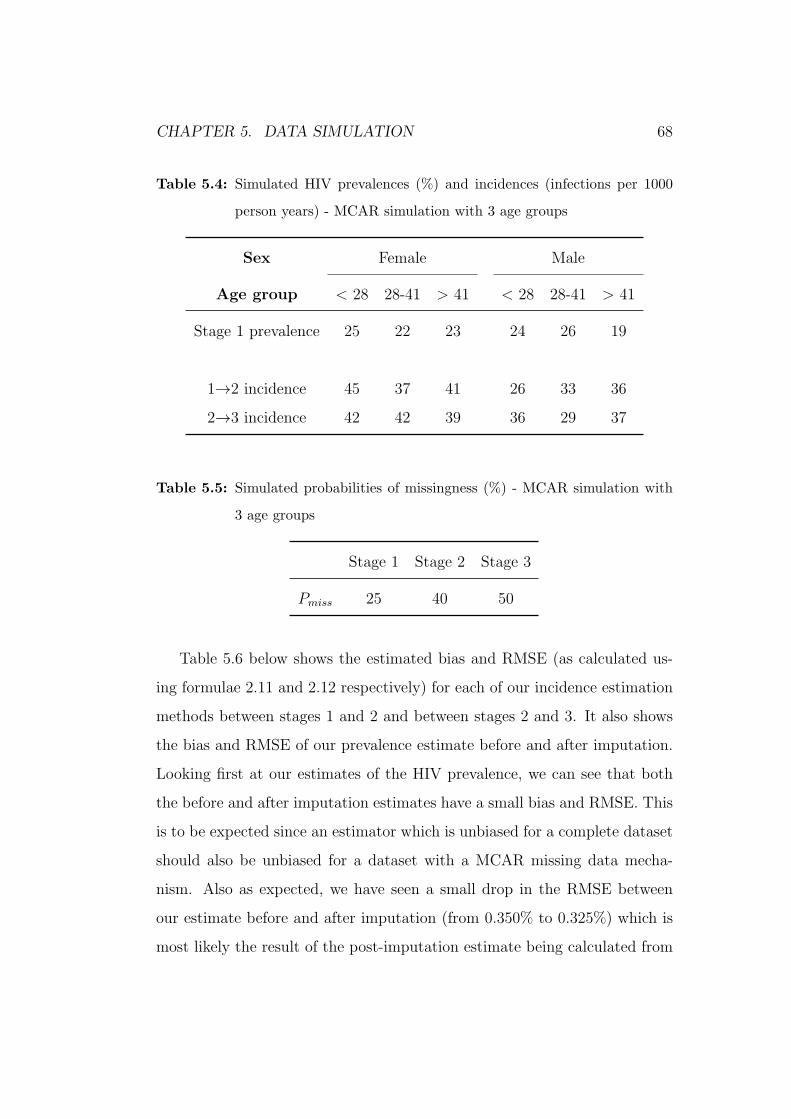
CHAPTER 5. DATA SIMULATION 68
Table 5.4: Simulated HIV prevalences (%) and incidences (infections per 1000
person years) - MCAR simulation with 3 age groups
Sex Female Male
Age group < 28 28-41 > 41 < 28 28-41 > 41
Stage 1 prevalence 25 22 23 24 26 19
1→2 incidence 45 37 41 26 33 36
2→3 incidence 42 42 39 36 29 37
Table 5.5: Simulated probabilities of missingness (%) - MCAR simulation with
3 age groups
Stage 1 Stage 2 Stage 3
Pmiss 25 40 50
Table 5.6 below shows the estimated bias and RMSE (as calculated us-
ing formulae 2.11 and 2.12 respectively) for each of our incidence estimation
methods between stages 1 and 2 and between stages 2 and 3. It also shows
the bias and RMSE of our prevalence estimate before and after imputation.
Looking first at our estimates of the HIV prevalence, we can see that both
the before and after imputation estimates have a small bias and RMSE. This
is to be expected since an estimator which is unbiased for a complete dataset
should also be unbiased for a dataset with a MCAR missing data mecha-
nism. Also as expected, we have seen a small drop in the RMSE between
our estimate before and after imputation (from 0.350% to 0.325%) which is
most likely the result of the post-imputation estimate being calculated from

CHAPTER 5. DATA SIMULATION 69
a larger sample size (with missing values now having been imputed).
Focussing now on the incidence between stages 1 and 2, we can see that
the two methods which perform best are the crude method and our impu-
tation method. Both have small biases, with our imputation method per-
forming slightly better in this respect (a bias of 0.07 compared to the crude
method’s bias of -0.148). The RMSE of these two methods is also smaller
than any of the others, while being fairly similar to one another (2.002 and
2.047 respectively). Parekh’s method also performs quite well with a bias
and RMSE of 0.214 and 3.515 respectively. The crudest method does not
perform quite so favourably with a bias of -6.9 infections per 1000 person
years.
Looking at the results for the incidence between stages 2 and 3, we see
that they are similar to those observed for stages 1 to 2. In terms of bias,
our imputation method performs marginally better than the others with a
bias of -0.11 with the crude and Parekh methods not far behind (biases of
-0.14 and -0.29 respectively). The crudest method has again been shown to
be incredibly biased with a bias of -19.5 infections per 1000 person years. In
terms of RMSE, the crude method and our imputation method perform very
similarly to one another with Parekh’s method once again not far behind.
Yet again , the crudest method has performed particularly badly with a very
large RMSE.

CHAPTER 5. DATA SIMULATION 70
Table 5.6: Bias and RMSE from simulation with imputation
Estimator Bias RMSE
Stage 1 Prevalence (%)
Before Imputation 0.007 0.350
After Imputation 0.002 0.325
1 → 2 Incidence (Infections per 1000 person years)
Crudest -6.872 7.067
Crude -0.148 2.002
Parekh 0.214 3.515
Imputation Method -0.070 2.047
2 → 3 Incidence (Infections per 1000 person years)
Crudest -19.475 19.533
Crude -0.142 3.052
Parekh -0.292 3.838
Imputation Method -0.109 3.123
In addition to the results which are presented above, we carried out an-
other 2 MCAR simulations. These simulations were similar but had 2 and 4
age groups (4 and 8 age-sex groups) by which the incidence and prevalence
differed. The results from these were similar to those seen already with the
imputation method performing the best and to a similar or marginally better

CHAPTER 5. DATA SIMULATION 71
level than the crude method. Again, these methods were closely followed by
the Parekh method which had a small bias and RMSE. The crudest method
did not perform well in any of our MCAR simulations. The results of these
two simulations are presented in appendix B.
From our MCAR simulations, it is quite evident that the crude method
and our imputation method are the least biased of all the methods which
we have studied here. The Parekh method also performs well. The crudest
method, which does not take time between tests into account, has proven to
be quite biased. Although this is as expected since we know that the average
time between tests - particularly between stages 1 and 2 - is far from a year
as this formula assumes.
5.8 MAR Simulations
Having completed our MCAR simulations, both the crude and imputation
methods have performed as expected under a MCARmissing data mechanism
in that both have proven to be approximately unbiased so far. The Parekh
method has also been shown to have small bias. With the introduction of
MAR missing data mechanisms in our next simulations, we might expect to
see the bias of some of our methods increase. In particular, we would expect
to see the introduction of some bias with our crude method since it does not
take account of the different levels of missingness within different groups in
the data.
5.8.1 MAR simulation with 2 age groups
Our first MAR simulation will contain 2 age groups, thereby allowing the
prevalence, incidence and missingness to differ by 4 age-sex groups. Table

CHAPTER 5. DATA SIMULATION 72
5.7 shows the prevalences and incidences within each age-sex group.
Table 5.7: Simulated HIV prevalences (%) and incidences (infections per 1000
person years) - MAR simulation with 2 age groups
Sex Female Male
Age group < 35 ≥ 35 < 35 ≥ 35
Stage 1 prevalence 16 23 21 24
1→2 incidence 15 35 36 28
2→3 incidence 36 69 31 55
As we are now simulating a missing at random dataset, the probability
of missingness varies by age-sex group as well as by testing stage. These
probabilities are detailed in table 5.8 below. The differences in the level of
missingness between each age-sex group in this simulation are reasonably
large and, as a consequence, we would expect that those methods which do
not take the missing data mechanism into account will display a reasonable
amount of bias. A glance at tables 5.7 and 5.8 and we notice that the stage
2 to 3 incidence is particularly high for males aged 35 or over while the
probability of missingness at stage 3 for this same group of individuals is
particularly low. As a consequence, we might expect those estimates of the
stage 2 to 3 incidence produced using methods which do not take the missing
data mechanism into account to be heavily influenced by this age-sex group
and, therefore, be particularly biased.

CHAPTER 5. DATA SIMULATION 73
Table 5.8: Probabilities of missingness by stage and age-sex group (%) - MAR
simulation with 2 age groups
Sex Female Male
Age group < 35 ≥ 35 < 35 ≥ 35
Stage 1 32 38 15 13
Stage 2 11 8 11 42
Stage 3 44 1 43 46
Using the parameters detailed in tables 5.7 and 5.8 to execute a sim-
ulation, we produce the bias and RMSE estimates for our prevalence and
incidence estimation methods detailed in table 5.9 below. In this scenario,
our imputation method performs best with the smallest bias and RMSE es-
timates at each stage. The next best performers are the crude and Parekh
methods with the Parekh method having a smaller bias than the crude for
the stage 1 to 2 incidence but the crude method having the smaller RMSE
in both cases. These results are more or less as expected given that we have
now moved from a MCAR to a MAR missing data mechanism meaning that
we would expect to see an increase in the bias of the crude method, or indeed
any method which doesn’t take the missingness into account. We should also
note that the bias and RMSE of some of our methods have increased between
the stages 1 to 2 estimates and the stages 2 to 3 estimates. It is possible
that this is due, at least in part, to the particularly high 2 to 3 incidence and
particularly low missingness for males aged over 35 as mentioned previously.
So, we can see that under a MAR missing data mechanism, just one group
of individuals can have a large effect on the accuracy of incidence estimates
which do not take the missingness into account.

CHAPTER 5. DATA SIMULATION 74
Table 5.9: Bias and RMSE from simulation with imputation - MAR simulation
with 2 age groups
Estimator Bias RMSE
Stage 1 Prevalence (%)
Before Imputation 0.231 0.393
After Imputation -0.009 0.285
1 → 2 Incidence (Infections per 1000 person years)
Crudest 4.497 4.770
Crude 0.481 1.451
Parekh -0.158 2.399
Imputation Method -0.013 1.353
2 → 3 Incidence (Infections per 1000 person years)
Crudest -15.655 15.712
Crude 1.090 2.494
Parekh 1.361 3.798
Imputation Method -0.005 2.330
5.8.2 MAR simulation with 3 age groups
Our next missing at random simulation has HIV prevalence, incidence
and missingness which differs according to 3 age groups and the gender of

CHAPTER 5. DATA SIMULATION 75
the individual. The HIV prevalences and incidences are detailed in table
5.10 below. Looking at this table we notice that the values are slightly more
consistent with one another than those in our previous simulation (table 5.7)
and there are no unusually large values as was the case previously. As such,
we may expect lower biases than were observed in our MAR simulation with
2 age groups.
Table 5.10: Simulated HIV prevalences (%) and incidences (infections per 1000
person years) - MAR simulation with 3 age groups
Sex Female Male
Age group < 28 28-41 > 41 < 28 28-41 > 41
Stage 1 prevalence 25 22 23 24 26 19
1→2 incidence 45 37 41 26 33 36
2→3 incidence 42 42 39 36 29 37
The probabilities of being classified as missing at each stage are detailed
in table 5.11. As with table 5.10 above, we notice that the values are reason-
ably consistent with one another and there are no extreme values such as the
1% probability of missingness for males aged over 35 in our MAR simulation
with 2 age groups (table 5.8). Again, we may expect to this to result in less
biased estimates than those seen in our previous simulation.

CHAPTER 5. DATA SIMULATION 76
Table 5.11: Probability of missingness by stage and age-sex group (%) - MAR
simulation with 3 age groups
Sex Female Male
Age group < 28 28-41 > 41 < 28 28-41 > 41
Stage 1 25 24 21 23 26 20
Stage 2 21 23 17 24 21 19
Stage 3 30 29 30 29 27 26
The bias and RMSE estimated by the simulations which were carried out
using the parameters detailed in tables 5.10 and 5.11 above are shown in
table 5.12 below. The first thing we notice when looking at this table is
that the bias of our crude method is much smaller than that observed in our
previous MAR simulation (section 5.8.1). The reason for this is apparent if
we look again at table 5.11 and notice that the probabilities of missingness
do not differ greatly between age and sex group. At each stage, there is
never more than 6% difference in the minimum and maximum probability of
missingness. These reasonably small differences in the level of missingness
between age and sex groups mean that our simulation is not too far removed
from a MCAR dataset which would explain the small bias observed with our
crude method.
As with our MCAR simulations, the best performing methods are our
imputation method and the crude method. Also like our MCAR simulations,
these two methods were closely followed by Parekh’s. The crudest method
displays a reasonable amount of bias.

CHAPTER 5. DATA SIMULATION 77
Table 5.12: Bias and RMSE from simulation with imputation
Estimator Bias RMSE
Stage 1 Prevalence (%)
Before Imputation -0.027 0.348
After Imputation 0.004 0.323
1 → 2 Incidence (Infections per 1000 person years)
Crudest 2.262 2.869
Crude 0.033 1.663
Parekh 0.458 3.106
Imputation Method -0.024 1.602
2 → 3 Incidence (Infections per 1000 person years)
Crudest -11.545 11.637
Crude 0.017 2.085
Parekh -0.039 3.181
Imputation Method 0.079 2.084
5.8.3 MAR simulation with 4 Age groups
Our next simulation is, again, similar to those which have proceeded it
but with an increased number of age-sex groups by which the missingness,
prevalence and incidence differ. We now have 8 age-sex groups with inci-

CHAPTER 5. DATA SIMULATION 78
dences and prevalences as detailed in table 5.13 below. As before, we have
chosen prevalences and incidences which are reasonably similar to those ob-
served in our original dataset.
Table 5.13: Simulated HIV prevalences (%) and incidences (infections per 1000
person years) - MAR simulation with 4 age groups
Sex Female Male
Age group < 25 25-34 35-44 ≥ 45 < 25 25-34 35-44 ≥ 45
Stage 1 prevalence 12 17 23 25 22 18 35 24
1→2 incidence 26 22 30 25 35 37 37 15
2→3 incidence 23 22 22 29 33 35 36 16
For this simulation, we have purposely ensured that there are noticeable
differences in the level of missingness in each of our age-sex groups in order
to ensure that we can test how the methods perform under a truly MAR
missing data mechanism. The probabilities of missingness are detailed in
table 5.14 below.

CHAPTER 5. DATA SIMULATION 79
Table 5.14: Probabilities of missingness by stage and age-sex group (%) - MAR
simulation with 4 age groups
Sex Female Male
Age group < 25 25-34 35-44 ≥ 45 < 25 25-34 35-44 ≥ 45
Stage 1 45 23 43 19 28 7 6 24
Stage 2 28 31 29 31 44 37 33 35
Stage 3 35 44 24 30 22 21 37 25
Using the parameters detailed above to run a simulation, we produce the
bias and RMSE estimates for each of our methods detailed in table 5.15. In
terms of the stage 1 prevalence, our imputation method clearly outperforms
the pre-imputation estimate with a much smaller bias and RMSE. However,
when we look at the stage 1 to 2 incidence, the crude method and our im-
putation method both perform very similarly in terms of bias and RMSE.
This is not the case with the stage 2 to 3 incidence though, with the bias and
RMSE of our imputation method much lower than that of the crude method.
Interestingly, the bias of the Parekh method at stages 2 to 3 is slightly lower
than that of our imputation method despite being noticeably larger at stages
1 to 2. Despite this, our imputation method still has the smaller RMSE and
since the bias is very low in both cases we would still consider this method
to be that which performs the best in this simulation given that it performs
consistently well.

CHAPTER 5. DATA SIMULATION 80
Table 5.15: Bias and RMSE from simulation with imputation
Estimator Bias RMSE
Stage 1 Prevalence (%)
Before Imputation 0.991 1.049
After Imputation 0.007 0.304
1 → 2 Incidence (Infections per 1000 person years)
Crudest -3.436 3.747
Crude 0.032 1.681
Parekh -0.360 2.829
Imputation Method 0.029 1.612
2 → 3 Incidence (Infections per 1000 person years)
Crudest -9.201 9.296
Crude -0.372 1.981
Parekh -0.026 2.762
Imputation Method 0.072 2.000
5.8.4 MAR simulation with low HIV prevalence and
incidences
The method of imputation method which we have developed in the course
of this study has so far been applied only to datasets with reasonably high

CHAPTER 5. DATA SIMULATION 81
HIV prevalences and incidences. These values were chosen to be reasonably
consistent with those observed in our original dataset. As such, it would be
of interest to investigate how it, and other methods, perform when applied
to data with comparatively low incidences and prevalences of HIV. This will
enable us to see how each method performs when applied to a dataset which
is purposely different from our own. Our next simulation is a MAR with 4
age groups and has HIV-incidences and prevalences as detailed in table 5.16
below.
Table 5.16: Simulated HIV prevalences (%) and incidences (infections per 1000
person years) - MAR simulation with low incidences
Sex Female Male
Age group < 25 25-34 35-44 ≥ 45 < 25 25-34 35-44 ≥ 45
Stage 1 prevalence 7 2 7 4 10 3 3 0
1→2 incidence 5 6 7 7 2 3 8 7
2→3 incidence 2 2 5 10 7 4 1 6
The probabilities of missingness for this simulation are shown in table
5.17 below. These have been maintained around about the same level as our
previous simulations so as to improve our ability to determine the effect of
low incidences on the accuracy of each of the methods.
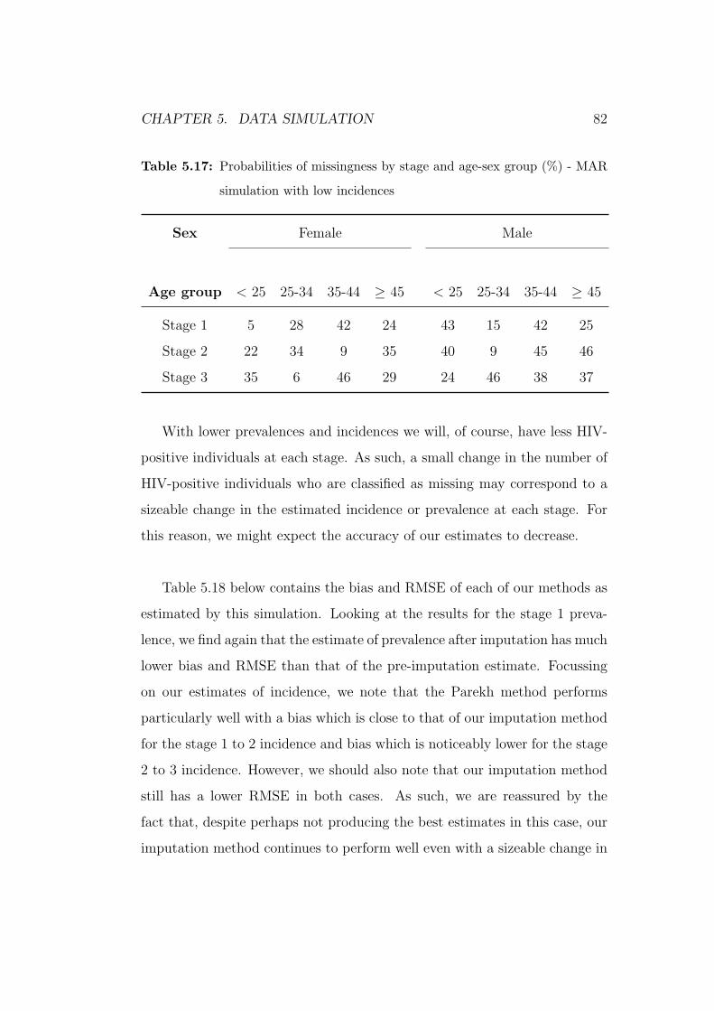
CHAPTER 5. DATA SIMULATION 82
Table 5.17: Probabilities of missingness by stage and age-sex group (%) - MAR
simulation with low incidences
Sex Female Male
Age group < 25 25-34 35-44 ≥ 45 < 25 25-34 35-44 ≥ 45
Stage 1 5 28 42 24 43 15 42 25
Stage 2 22 34 9 35 40 9 45 46
Stage 3 35 6 46 29 24 46 38 37
With lower prevalences and incidences we will, of course, have less HIV-
positive individuals at each stage. As such, a small change in the number of
HIV-positive individuals who are classified as missing may correspond to a
sizeable change in the estimated incidence or prevalence at each stage. For
this reason, we might expect the accuracy of our estimates to decrease.
Table 5.18 below contains the bias and RMSE of each of our methods as
estimated by this simulation. Looking at the results for the stage 1 preva-
lence, we find again that the estimate of prevalence after imputation has much
lower bias and RMSE than that of the pre-imputation estimate. Focussing
on our estimates of incidence, we note that the Parekh method performs
particularly well with a bias which is close to that of our imputation method
for the stage 1 to 2 incidence and bias which is noticeably lower for the stage
2 to 3 incidence. However, we should also note that our imputation method
still has a lower RMSE in both cases. As such, we are reassured by the
fact that, despite perhaps not producing the best estimates in this case, our
imputation method continues to perform well even with a sizeable change in

CHAPTER 5. DATA SIMULATION 83
the parameter which it was designed to estimate.
Table 5.18: Bias and RMSE from simulation with imputation (Simulation with
low incidence and prevalence)
Estimator Bias RMSE
Stage 1 Prevalence (%)
Before Imputation -0.145 0.245
After Imputation 0.006 0.180
1 → 2 Incidence (Infections per 1000 person years)
Crudest -0.012 0.557
Crude 0.076 0.570
Parekh 0.048 1.008
Imputation Method -0.042 0.572
2 → 3 Incidence (Infections per 1000 person years)
Crudest -1.483 1.546
Crude -0.106 0.677
Parekh 0.035 0.993
Imputation Method 0.102 0.698

CHAPTER 5. DATA SIMULATION 84
5.8.5 MAR simulation with small sample size
In line with the size of our original dataset, all of our simulations so far
have been performed using a dataset with a reasonably large number of in-
dividuals (20,000). It would be interesting to see if our methods of incidence
continue to perform to the same level when applied to a relatively small
dataset. In this simulation, we will be using a sample size of just 2000 and,
as such, we might expect the RMSE of our methods to increase given that all
estimates will be based on smaller sample sizes, which should increase their
variance. The prevalences and incidences, as we have done previously, were
chosen to be reasonably close to those which were observed in our original
data. These are detailed in table 5.19 below.
Table 5.19: Simulated HIV prevalences (%) and incidences (infections per 1000
person years) - MAR simulation with small sample size
Sex Female Male
Age group < 25 25-34 35-44 ≥ 45 < 25 25-34 35-44 ≥ 45
Stage 1 prevalence 23 27 11 21 24 10 26 13
1→2 incidence 28 32 17 27 23 24 32 20
2→3 incidence 27 20 28 31 24 32 23 31
Similarly to our incidences, the probabilities of missingness were chosen
so as to not be entirely dissimilar to those observed in the original dataset.
These are detailed in tabled 5.20 below.

CHAPTER 5. DATA SIMULATION 85
Table 5.20: Probabilities of missingness by stage and age-sex group (%) - MAR
simulation with small sample size
Sex Male Female
Age group < 25 25-34 35-44 ≥ 45 < 25 25-34 35-44 ≥ 45
Stage 1 13 26 28 15 33 34 9 19
Stage 2 31 14 40 21 32 25 28 40
Stage 3 17 14 39 34 32 14 22 29
Looking at the results for this simulation which are detailed in table 5.21
below, it is apparent that the Parekh method performs quite well with very
low bias estimates for both the stage 1 to 2 incidence and the stage 2 to 3
incidence. While our imputation method displays a bias which is large by
comparison, it is still reasonably low (0.33 for stages 1 to 2 and 0.45 for 2 to
3) which is reassuring given the small sample size. The crude method also
performs quite well with reasonably low biases, particularly for the stage 1
to 2 incidence estimate. As we expected, all methods also have an RMSE
which is larger than we have generally seen previously. This is, of course,
can be accredited to the greatly reduced sample size.
Once again, it is reassuring that, while not being the least biased method
in this simulation, our imputation method continues to perform well with
low biases and the lowest RMSEs of all the methods.

CHAPTER 5. DATA SIMULATION 86
Table 5.21: Bias and RMSE from simulation with imputation (MAR simulation
with small sample size)
Estimator Bias RMSE
Stage 1 Prevalence (%)
Before Imputation 0.201 1.071
After Imputation -0.039 0.956
1 → 2 Incidence (Infections per 1000 person years)
Crudest -0.764 4.506
Crude 0.408 4.631
Parekh 0.061 7.970
Imputation Method 0.330 4.246
2 → 3 Incidence (Infections per 1000 person years)
Crudest -6.524 7.787
Crude -0.031 5.607
Parekh -0.044 7.988
Imputation Method 0.451 5.392

CHAPTER 5. DATA SIMULATION 87
5.9 Brief summary of our simulation results
In carrying out our simulations we have noticed a number of patterns. In
our MCAR simulations, the crude method and our imputation method per-
formed to a similar level in terms of both bias and RMSE. These two methods
were closely followed by the Parekh method which also demonstrated a low
level of bias in most cases. The good performance of the crude method in
this scenario is as expected since estimates which are based on data with a
missing completely at random missing data mechanism should not require
any adjustment in order to obtain unbiased results.
It is when we move to MAR simulations that we start to see bias intro-
duced to the results which are produced by the crude method. Again, this
is as expected since the crude method makes no adjustments for the missing
data mechanism and, as such, should produce biased results.
The Parekh method continued to perform to a similar level as it had
with our MCAR simulations with a fairly low level of bias. We should note,
though, that in reality one would not know the exact value of the sensi-
tivity and specificity of the tests of recency which would introduce further
uncertainty to the estimates produced using the Parekh method. One of the
reasons the Parekh method performs quite well is that, while it does not
take the missingness into account, it uses the results from only one stage
of testing meaning it is only exposed to the missingness at that one stage
rather than at two stages as with the other methods. This is, at least partly,
why we sometimes see it perform well in estimating, say, the stage 1 to 2
incidence but then perform comparatively badly in estimating the stage 2 to
3 incidence. So, much like the crude method, it performs well when the prob-

CHAPTER 5. DATA SIMULATION 88
abilities of missingness are reasonably consistent across the age-sex groups
and relatively poorly when there is more variability in the probabilities of
missingness between age-sex groups. Unlike the crude method though, it is
less affected by the missingness since it doesn’t have to cope with a combi-
nation of missing values from two stages.
Our imputation method consistently produced estimates with bias and
RMSE which were among the lowest of any of the methods investigated.
However, when we began to perform MAR simulations with parameters that
differed greatly from those which were observed in our original data, we did
see small amounts of bias creep into some of the estimates which our im-
putation method produced. Even so, it still performed well with biases and
RMSE which were still reasonably small. As such, our imputation method is
the only which can be considered to have performed consistently well in all
of our simulations.
The crudest method did not perform well in any of our simulations. This
is as we would expect since it does not take the time between tests into
account.

Chapter 6
Conclusions
6.1 Summary of results
In the course of this study, we have looked at a number of different meth-
ods of estimating the incidence of HIV, each with its own merits. We began
with the crudest method of imputation which was described in section 2.1.1
(equation 2.1). While it is the simplest method of estimating incidence, it
is only useful when the data to which it is applied conforms to some strict
rules. Specifically, it only works effectively when each and every individual
in the dataset is tested once at baseline and then tested again after precisely
the same amount of time. This fact was demonstrated when it was applied to
our simulated datasets in a complete-case analysis and the bias and RMSE
for the crudest method were both noticeably higher than that for every other
method in almost every simulation.
It was for this reason that we introduced our second method incidence
estimation, the crude method as described in section 2.2 (equation 2.3). This
formula takes the time between tests into account and, as such, should per-
89

CHAPTER 6. CONCLUSIONS 90
form better in circumstances, such as ours, where the time between each indi-
vidual’s test is not exactly the same. When applied to our original dataset in
a complete-case analysis, it provided estimates of the incidence between dif-
ferent stages which were much more consistent with one another than those
calculated using the crudest method of incidence estimation. This would im-
ply that (as we would expect) this method is more accurate than the crudest
method of incidence estimation. This is demonstrated by our MCAR sim-
ulations, where, in a complete-case analysis, this method performs well and
proves to be unbiased and have a small RMSE. However, this method does
not take into account the missing test results and can return biased estimates
of the incidence when the missing data mechanism is not MCAR. Again, this
fact is demonstrated by the complete-case analyses in our simulations when
the bias of this method increases noticeably when we move from MCAR sim-
ulations to MAR simulations.
Next, we began to investigate the Parekh and McDougal methods as de-
scribed in sections 2.4.1 and 2.4.2 respectively. These methods are useful in
that they do not require test results at two separate time points. Instead,
they use the results from a single test to estimate whether or not each HIV-
positive individual seroconverted within a designated time frame prior to the
test (153 days in our case). However, both these methods make a number of
assumptions about the data. They rely heavily on measures of the accuracy
of the test, which can be difficult to estimate. In our simulation studies,
where we knew exactly the accuracy of the test results (i.e. the sensitivity
and the specificity), the Parekh formula performed reasonably well in terms
of having a small bias and RMSE. This would certainly suggest that such
methods can be effective if measures such as the sensitivity and specificity

CHAPTER 6. CONCLUSIONS 91
can be estimated with a high degree of precision. Though, it is possible be
that our simulation method favoured these methods by the manner in which
we simulated recency. When applied to our original data, we note that it
can produce some abnormally low estimates of the incidence (see tables 3.6
and 3.9). Both these methods produce estimates of the incidence between
stages 2 and 3 of around 2 to 5 infections per 1000 person years. Such low
estimates may suggest that, while these methods can work well under certain
conditions, they are somewhat incompatible with our data which.
The next step was to develop a method of HIV incidence of our own. For
this we imputed the HIV test results within each age-sex group depending
on the incidence and prevalence of HIV in each of these groups (as described
in chapter 4). Applying this to our original dataset decreased our 1 → 2 inci-
dence estimate (as calculated using the crude method) and slightly increased
our 2 → 3. This brought the two estimates approximately in line with each
other whereas previously there was a difference of about 4 infections per 1000
person years between them. When applied to our simulated data sets, this
method was shown to be amongst the least biased in every case with a couple
of exceptions where extreme values of parameters were used.
With regards to our original data, there can be little doubt that our im-
putation method is the preferred method of incidence estimation of those
investigated in the course of this study. The crudest method was almost
immediately discounted as a credible means of incidence estimation since
it does not take the length of time between HIV tests into account. The
crude method produced more realistic estimates of the incidence, however,
it’s estimate of the incidence between stage 1 and stage 3 was lower than the

CHAPTER 6. CONCLUSIONS 92
estimate it produced for both the stages 1 to 2 incidence and stages 2 to 3
incidence. Of course, the stages 1 to 3 incidence should lie between the 1 to
2 incidence and the 2 to 3 incidence. As such, it is clear that these estimates
of the incidence have been affected by the missing values in the data. Both
the McDougal and Parekh methods produced estimates of the incidence be-
tween stages 2 and 3 and between 1 and 3 which were impossibly low. This
is indicative of either a serious problem with the OD values at stage 3 or
some major response bias. Our imputation method did not show any such
bizarre results and performed consistently well in our chapter 5 simulations.
Using our imputation method, our best estimate of the HIV incidence
between stages 1 and 2 is 31.04 infections per 1000 person years with a
95% confidence interval of 30.25 to 31.83 infections per 1000 person years.
Our best estimate of the HIV incidence between stages 2 and 3 is 30.92
infections per 1000 person years with a 95% confidence interval of 29.72 to
32.13 infections per 1000 person years. Our imputation method also produces
the best estimate of the HIV incidence between stages 1 and 3 of 30.96
infections per 1000 person year with a 95% confidence interval of 30.46 to
31.47 infections per 1000 person years.
6.2 Limitations of the study
In developing our method of incidence estimation, we assumed a MAR
missing data mechanism in our dataset. However, there exists the very real
possibility that the mechanism was NMAR, that is, the missingness depends
on the HIV test results. For example, this could arise if an individual knows
or suspects that they have become HIV-positive since their last negative test

CHAPTER 6. CONCLUSIONS 93
result and, for this reason, refuses to be re-tested. Unfortunately, data which
are not missing at random are very difficult to impute since the probability
of missingness depends on the missing value itself.
In applying the McDougal and Parekh methods, we relied heavily on mea-
sures of the accuracy of the test. Specifically, we required knowledge about
the sensitivity, specificity and the long- and short-term false positive ratios.
Ideally, we would have been able to use the OD values and the times from
seroconversion to test date in order to produce our own estimates of the test
specificity and sensitivity as well as choose our own OD cut-off definition of
recency. In order to do this, we would need to know with a fair degree of
precision the between seroconversion and HIV testing. In addition to this,
we would require a wide variety in the length of times - from a matter of
days to a matter of months - between seroconversion and testing in order
to choose an appropriate definition of recency and corresponding OD cut-off
value. Unfortunately, neither of these conditions is met since our best esti-
mate of the time from seroconversion to testing is the mid-point between the
last negative and first positive HIV test and the times between tests are typ-
ically around a year or greater. As such, we are forced to rely on estimates
of the specificity, sensitivity and long- and short-term false positive ratios
from elsewhere which may not be compatible with the data in our study. If
the true values of these measures differ to those which were used, they will
adversely affect our estimates of the incidence. It should be noted, however,
that our simulation study did show that the Parekh method performed quite
well when the true value of the sensitivity and specificity are known.
It also became quite apparent in our chapter 3 analysis that there is some-

CHAPTER 6. CONCLUSIONS 94
thing quite erroneous about the OD values seen at the third stage of testing.
This resulted in some very low results when estimating both the 2 to 3 and
1 to 3 incidence using McDougal and Parekh methods. As such, we were
left with little confidence in these results and were left unable to test the
McDougal or Parekh method on an appropriate real-world dataset.
The method of imputation developed in this study was designed to make
the most of the data which were available to us. In addition to this, we
observed a slight drop in accuracy when we applied this imputation method
to simulated datasets which were somewhat dissimilar to our own. As such,
it would be unwise to attempt to draw any conclusions about the application
of this method to a wider range of datasets.
6.3 Further Work
There are a number of ways in which the work completed in this study
could be carried forward. One aspect that is worthy of further investigation
is the use of the OD value as an indicator of recency. It is incredibly useful in
that it can be used to produce an estimate of the incidence using the results
from only one test at one time point. It is this relationship with time that is
of the most interest. That the OD value increases with time would suggest
that there could be some means of modelling the relationship between the
two. If this could be achieved, one could then produce estimates of the time
since seroconversion at the testing date for each individual in a given dataset.
This would also mean that we would be making better use of the available
information in that each individual would have their own estimate of time
since seroconversion instead of simply being classified as recently or not re-

CHAPTER 6. CONCLUSIONS 95
cently infected. By dropping the use of recent/non-recent classification, we
would also avoid the issue of false-positives and false-negatives, thereby re-
moving the need for (difficult) estimation of sensitivity, specificity and long-
and short-term false positive ratios. This was an option which was considered
early in our own study, unfortunately we were unable to obtain appropriate
data.
In addition to this, different methods of imputation could be attempted.
Specifically, we could impute all missing values probabilistically, missing out
the deterministic step altogether. The manner in which we impute proba-
bilistically could also be adjusted. Instead of estimating the probability from
the original dataset, we could have drawn the estimate for each imputation
separately from a distribution of possible probability values. For example,
we could set up a uniform distribution for the probabilities on an interval
around the ‘best’ estimate and draw a probability from it each time or con-
struct a confidence interval for the probability and draw from it each time.
Of course, possible further work could also include the application of the
methods investigated here to other HIV datasets and comparing the results
estimates of the HIV incidence which already exist for those datasets. This
would be particularly useful since, at present, our method of imputation is
quite specific to our own dataset since it was designed to make optimum use
of the data which was available to us.
Appendix A
Additional multiple imputation
results
96

APPENDIX A. ADDITIONAL MULTIPLE IMPUTATION RESULTS 97
Table
A.1:Incidence
estimates
from
multiple
imputationwithoutagegrouping(infectionsper
1000personyears)
1→2incidence
2→3incidence
1→3incidence
Imputation
Estim
ate
Variance
Estim
ate
Variance
Estim
ate
Variance
127.44
1.40
28.02
2.04
27.67
0.83
227.82
1.42
28.76
2.11
28.22
0.85
327.90
1.42
29.69
2.16
28.64
0.86
428.29
1.44
29.85
2.17
28.93
0.86
527.81
1.41
30.19
2.21
28.80
0.86
627.58
1.41
26.86
1.94
27.27
0.81
728.94
1.47
28.16
2.05
28.60
0.85
827.38
1.39
30.83
2.24
28.82
0.86
927.26
1.39
28.24
2.05
27.66
0.83
1027.06
1.38
28.51
2.08
27.66
0.83
MeanEst.(95%
C.I.)
27.75
(27.12,28.38)
28.91
(27.72,30.10)
28.23
(27.72,28.73)

APPENDIX A. ADDITIONAL MULTIPLE IMPUTATION RESULTS 98
Table
A.2:Incidence
estimates
from
multiple
imputationusing2agegroups(infectionsper
1000personyears)
1→2incidence
2→3incidence
1→3incidence
Imputation
Estim
ate
Variance
Estim
ate
Variance
Estim
ate
Variance
128.13
1.43
30.89
2.26
29.27
0.88
227.51
1.39
30.91
2.27
28.92
0.87
328.64
1.46
30.27
2.21
29.31
0.88
430.40
1.54
27.88
2.03
29.33
0.87
527.41
1.40
30.41
2.23
28.65
0.86
629.09
1.47
29.74
2.15
29.35
0.87
728.22
1.43
29.68
2.18
28.82
0.86
828.39
1.45
26.74
1.96
27.68
0.83
929.72
1.05
31.01
2.27
30.25
0.90
1028.95
1.47
28.78
2.10
28.86
0.86
MeanEst.(95%
C.I.)
28.64
(27.70,29.59)
29.63
(28.29,30.98)
29.04
(28.51,29.58)

APPENDIX A. ADDITIONAL MULTIPLE IMPUTATION RESULTS 99
Table
A.3:Incidence
estimates
from
multiple
imputationusing3agegroups(infectionsper
1000personyears)
1→2incidence
2→3incidence
1→3incidence
Imputation
Estim
ate
Variance
Estim
ate
Variance
Estim
ate
Variance
130.53
1.65
32.63
2.43
31.39
0.98
228.57
1.52
29.89
2.24
29.10
0.90
328.49
1.51
31.20
2.35
29.60
0.92
429.92
1.62
29.99
2.24
29.93
0.94
528.10
1.50
30.91
2.29
29.25
0.90
629.23
1.57
29.51
2.17
29.34
0.91
728.39
1.52
30.63
2.29
29.32
0.91
831.64
1.69
32.77
2.44
32.09
1.00
929.42
1.58
29.53
2.19
29.45
0.92
1030.31
1.62
29.07
2.15
29.78
0.92
MeanEst.(95%
C.I.)
29.46
(28.37,30.55)
30.61
(29.35,31.87)
29.93
(29.10,30.75)

APPENDIX A. ADDITIONAL MULTIPLE IMPUTATION RESULTS 100
Table
A.4:Incidence
estimates
from
multiple
imputationusing5agegroups(infectionsper
1000personyears)
1→2incidence
2→3incidence
1→3incidence
Imputation
Estim
ate
Variance
Estim
ate
Variance
Estim
ate
Variance
131.40
1.81
30.55
2.27
31.05
1.01
232.52
1.91
29.53
2.17
31.26
1.02
331.90
1.86
30.11
2.22
31.14
1.02
431.56
1.84
31.55
2.34
31.56
1.03
530.22
1.79
31.19
2.32
30.59
1.01
631.88
1.86
31.19
2.34
31.58
1.04
729.72
1.73
29.69
2.18
29.72
0.97
832.76
1.93
32.18
2.39
32.50
1.07
930.00
1.77
30.91
2.30
30.38
1.00
1032.69
1.9
30.50
2.25
31.74
1.03
MeanEst.(95%
C.I.)
31.47
(30.35,32.58)
30.74
(29.82,31.66)
31.15
(30.48,31.82)

APPENDIX A. ADDITIONAL MULTIPLE IMPUTATION RESULTS 101
Table
A.5:Incidence
estimates
from
multiple
imputationusing6agegroups(infectionsper
1000personyears)
1→2incidence
2→3incidence
1→3incidence
Imputation
Estim
ate
Variance
Estim
ate
Variance
Estim
ate
Variance
131.27
1.81
31.24
2.40
31.25
1.03
231.04
1.77
32.57
2.50
31.66
1.04
330.40
1.73
30.48
2.32
30.41
0.99
431.14
1.79
31.08
2.35
31.12
1.02
532.42
1.84
28.34
2.15
30.70
1.00
630.21
1.74
30.43
2.28
30.28
0.99
730.30
1.72
29.56
2.26
29.99
0.98
830.87
1.75
31.01
2.33
30.89
1.00
929.55
1.67
29.71
2.23
29.61
0.95
1031.59
1.80
29.51
2.23
30.70
1.00
MeanEst.(95%
C.I.)
30.88
(30.00,31.76)
30.39
(29.21,31.58)
30.66
(30.15,31.18)

Appendix B
Additional MCAR simulation
results
B.1 MCAR simulation with 2 age groups
Table B.1: Simulated HIV prevalences (%) and incidences (infections per 1000
person years) - MCAR simulation with 2 age groups
Sex Female Male
Age group < 35 ≥ 35 < 35 ≥ 35
Stage 1 prevalence 22.5 15 25 17.5
1→2 incidence 60 70 80 50
2→3 incidence 50 50 60 40
102

APPENDIX B. ADDITIONAL MCAR SIMULATION RESULTS 103
Table B.2: Bias and RMSE from simulation with imputation
Estimator Bias RMSE
Stage 1 Prevalence (%)
Before Imputation -0.005 0.333
After Imputation -0.011 0.317
1 → 2 Incidence (Infections per 1000 person years)
Crudest -13.408 13.576
Crude -0.273 2.586
Parekh 1.138 4.763
Imputation Method 0.068 2.571
2 → 3 Incidence (Infections per 1000 person years)
Crudest -27.151 27.206
Crude -0.200 3.492
Parekh -0.394 4.514
Imputation Method 0.086 3.528

APPENDIX B. ADDITIONAL MCAR SIMULATION RESULTS 104
B.2 MCAR simulation with 4 age groups
Table B.3: Simulated HIV prevalences (%) and incidences (infections per 1000
person years) - MCAR simulation with 4 age groups
Sex Female Male
Age group < 25 25-34 35-44 ≥ 45 < 25 25-34 35-44 ≥ 45
Stage 1 prevalence 17 24 27 19 18 22 27 16
1→2 incidence 40 43 51 48 36 42 29 34
2→3 incidence 38 41 43 49 42 37 34 53

APPENDIX B. ADDITIONAL MCAR SIMULATION RESULTS 105
Table B.4: Bias and RMSE from simulation with imputation
Estimator Bias RMSE
Stage 1 Prevalence (%)
Before Imputation -0.003 0.315
After Imputation 0.003 0.300
1 → 2 Incidence (Infections per 1000 person years)
Crudest -7.237 7.413
Crude 0.035 1.943
Parekh 0.297 3.379
Imputation Method 0.051 2.040
2 → 3 Incidence (Infections per 1000 person years)
Crudest -20.530 20.585
Crude -0.082 3.019
Parekh -0.237 4.133
Imputation Method -0.171 3.076

Bibliography
Barnighausen, T., Wallrauch, C., Welte, A., McWalter, T. A., Mbizana, N.,
Viljoen, J., Graham, N., Tanser, F., Puren, A. & Newell, M.-L. (2008),
‘HIV Incidence in Rural South Africa: Comparison of Estimates from
Longitudinal Surveillance and Cross-Sectional cBED Assay Testing’, PLoS
ONE 3, e3640.
Guidelines for Using HIV Testing Technologies in Surveillance: Selec-
tion, Evaluation, and Implementation (2001), http://data.unaids.org/
publications/IRC-pub02/jc602-hivsurvguidel_en.pdf.
Hargrove, J. W., Humphrey, J. H., Mutasa, K., Parekh, B. S., McDougal,
J. S., Ntozini, R., Chidawanyika, H., Moulton, L. H., Ward, B., Nathoo,
K., Iliff, P. J. & Kopp, E. (2008), ‘Improved HIV-1 incidence estimates
using the BED capture enzyme immunoassay’, AIDS 22(4), 511–518.
HIV and AIDS Strategy for the Province of KwaZulu-Natal 2006-2010 (2006),
Report, Office of the Premier, Pietermaritzburg, KwaZulu-Natal, South
Africa.
Little, R. J. A. & Rubin, D. B. (2002), Statistical Analysis with Missing
Data, Wiley series in probability and statistics, 2nd edn, John Wiley &
Sons, Inc.
106

BIBLIOGRAPHY 107
McDougal, J. S., Parekh, B. S., Peterson, M. L., Branson, B. M., Dobbs,
T., Ackers, M. & Gurwith, M. (2006), ‘Comparison of HIV Type 1 Inci-
dence Observed during Longitudinal Follow-Up with Incidence Estimated
by Cross-Sectional Analysis Using the BED Capture Enzyme Immunoas-
say’, Aids Research and Human Retroviruses 22(10), 945–952.
McWalter, T. A. & Welte, A. (2008), ‘Relating Recent Infection Prevalence
to Incidence with a Sub-population of Non-progressors’, http://arxiv.
org/abs/0801.3380. Accessed 22 February 2010.
Muhwava, W., Nyirenda, M., Mutevedzi, T., Herbst, K. & Hosegood, V.
(2007), Operational and Methodological Procedures of the Africa Centre
Demographic Information System, Monograph 1, Africa Centre for Health
and Population Studies, Somkhele, South Africa.
National HIV and Syphilis Antenatal Sero-Prevalence Survey in South Africa
2004 (2005), Report, Department of Health, Pretoria, South Africa.
Parekh, B., Kennedy, M., Dobbs, T., Pau, C., Byers, R., Green, T., Hu,
D., Vanichseni, S., Young, N., Choopanya, K., Mastro, T. & McDougal, J.
(2002), ‘Quantitative Detection of Increasing HIV Type 1 Antibodies after
Seroconversion: A Simple Assay for Detecting Recent HIV Infection and
Estimating Incidence’, Aids Research and Human Retroviruses 18(4), 295–
307.
World Health Organisation Website (2010), http://www.who.int/topics/
hiv_aids/en/. Accessed 25 January 2010.