MPRAMunich Personal RePEc Archive

Preference aggregation theory withoutacyclicity: The core without majoritydissatisfaction

Masahiro Kumabe and H. Reiju Mihara

The Open University of Japan, Kagawa University Library

July 2010

Online at https://mpra.ub.uni-muenchen.de/23918/MPRA Paper No. 23918, posted 16. July 2010 08:27 UTC

Preference aggregation theory without acyclicity:

The core without majority dissatisfaction∗

Masahiro KumabeFaculty of Liberal Arts, The Open University of Japan2-11 Wakaba, Mihama-ku, Chiba City, 261-8586 Japan

H. Reiju Mihara†

Kagawa University LibraryTakamatsu 760-8525, Japan

July 2010

Abstract

Acyclicity of individual preferences is a minimal assumption in so-cial choice theory. We replace that assumption by the direct assump-tion that preferences have maximal elements on a fixed agenda. Weshow that the core of a simple game is nonempty for all profiles of suchpreferences if and only if the number of alternatives in the agenda isless than the Nakamura number of the game. The same is true if wereplace the core by the core without majority dissatisfaction, obtainedby deleting from the agenda all the alternatives that are non-maximalfor all players in a winning coalition. Unlike the core, the core withoutmajority dissatisfaction depends only on the players’ sets of maximalelements and is included in the union of such sets. A result for anextended framework gives another sense in which the core withoutmajority dissatisfaction behaves better than the core.

Journal of Economic Literature Classifications: C71, D71, C02.Keywords: Core, Nakamura number, kappa number, simple games,

voting games, maximal elements, acyclic preferences, limit ordinals.

∗Games and Economic Behavior (2010), doi:10.1016/j.geb.2010.06.008.†Corresponding author.

URL: http://econpapers.repec.org/RAS/pmi193.htm (H.R. Mihara).

1

1 Introduction

1.1 Preference aggregation theory for acyclic individual pref-erences

Preference aggregation theory is concerned with aggregating individual pref-erences into a (collective) social preference, which is then maximized to yielda set of best alternatives. The theory investigates the extent to which so-cial preferences inherit desirable properties from individual preferences. Wetypically restrict (strict) individual and social preferences to those asym-metric relations � on a set X of alternatives that are either (i) acyclic or(ii) transitive or (iii) negatively transitive.1

Of the properties (i), (ii), and (iii) for asymmetric preferences, negativetransitivity is the most demanding. Arrow’s Theorem (1963) points out thedifficulty of aggregating preferences for more than two alternatives whilepreserving asymmetry and negative transitivity.2

Acyclicity is the least demanding of the properties; it is necessary andsufficient for the existence of a maximal element on every finite subset ofalternatives. The Nakamura number plays a critical role in the study of pref-erence aggregation rules with acyclic social preferences.3 Consider a simplegame (voting game) W, a collection of “winning” coalitions in a set N ofplayers. Combining the game with a set X of alternatives and a profilep = (�p

i )i∈N of individual preferences, one obtains a simple game withpreferences (W, X,p), for which one can define the social preference �p

W(dominance relation) and the core C(W, X,p) (the set of maximal alterna-tives with respect to �p

W). Nakamura’s theorem (1979) gives a restrictionon the number of alternatives that the set of players can deal with rationally(Theorem 1): the core of a simple game with preferences is always (i.e., forall profiles of acyclic preferences) nonempty if and only if the number of al-ternatives is finite and below a certain number, called the Nakamura numberof the simple game. The theorem thus gives a condition (Corollary 1) forthe social preferences to inherit acyclicity from individual preferences.

1Define the weak preference � by x � y ⇔ y 6� x. � is asymmetric iff � is complete(reflexive and total). (i) � is acyclic if for any finite set {x1, x2, . . . , xm} ⊆ X, wheneverx1 � x2, . . . , xm−1 � xm, we have xm 6� x1. If � is acyclic, it is asymmetric andirreflexive. (ii) � is transitive if x � y and y � z imply x � z. When � is transitive, wesay � is quasi-transitive. (iii) � is negatively transitive if x 6� y and y 6� z imply x 6� z.� is negatively transitive iff � is transitive.

2The restriction to two alternatives disappears when there are infinitely many individ-uals (Fishburn, 1970), but such a resolution relies on highly nonconstructive mathematicalobjects (Mihara, 1997, 1999).

3Banks (1995), Truchon (1995), Andjiga and Mbih (2000), and Kumabe and Mihara(2008a) are recent contributions to the literature. Earlier papers on acyclic rules canbe found in Truchon (1995) and Austen-Smith and Banks (1999). Kumabe and Mihara(2008b) comprehensively study the restrictions that various properties for a simple gameimpose on its Nakamura number.

2

To deal with an empty core (or cycles in social preferences), severalauthors have investigated solutions different from the core. We pick twoexamples for which there have been recent developments. First, Duggan(2007) proposes a procedure in which one deletes particular instances ofpreferences until the resulting subrelation is acyclic (alternatively, transi-tive or negatively transitive), and collects the maximal elements of all such(maximal acyclic) subrelations.4 Second, taking voters’ foresight into con-sideration, Rubinstein (1980) proposes the stability set, a superset of thecore.5 All these investigations focus on treating cyclic social preferences,assuming that individual preferences satisfy a rationality property at leastas strong as acyclicity.

1.2 Preference aggregation theory without acyclicity

In this paper, we propose a preference aggregation theory without acyclicity.In contrast to the authors cited in the preceding paragraph, we do notattempt to remove cycles in (social and even individual) preferences.

We retain the usual framework (e.g., Arrow, 1963, Section II.2) in whicha set X of underlying alternatives is distinguished from an agenda (oppor-tunity set) B ⊆ X with which a group N of players are confronted. Inparticular, fixing a simple game W and a set X, we focus on the aggrega-tion methods that assign the core C(W, B,p) or the core without majoritydissatisfaction C+(W, B,p) (introduced later)6 to each (W, B,p) satisfyinga certain assumption. The assumption, which is actually a condition con-cerning a pair (B,p), is that every player’s preference �p

i has a maximalelement in B: the maximal set maxB �p

i (the set of maximal elements ofthe preference) is nonempty for each i.7 This is a rather direct assumptionat the individual level, which is to be inherited to the requirement at thesocial level that there is a chosen alternative for the given pair.

The assumption is distinctive in that it involves an agenda B as well asa profile p. For this reason, it does not fit the following Standard Scenario

4A related procedure is to collect the maximal elements of all maximal chains (subsetsof alternatives on which the majority preference is a linear order), which yields the Banksset (Banks, 1985; Penn, 2006); the set consists of the sophisticated voting outcomes ofsome binary agenda.

5Le Breton and Salles (1990) provide a sufficient condition for the general nonemptynessof the stability set in terms of the Nakamura number. Using more complex characteristicnumbers, Martin and Merlin (2006) propose a weaker sufficient condition and Andjigaand Moyouwou (2006) a necessary and sufficient condition for the general nonemptynessof the stability set.

6As the notation suggests, we define the core (without majority dissatisfaction) relativeto an agenda B.

7Acyclicity of a preference is independent of the property of having a maximal element.There is a cyclic preference that has a maximal element on X. When X is infinite, there isan acyclic preference that has no maximal element on X. Similarly, the property of havinga maximal element on B is independent of the property of having a maximal element on X.

3

in social choice theory (Arrow, 1963, page 12) very well: before knowingan agenda, the players discover and report their own preferences (on X) tothe planner; having obtained a choice rule that assigns a nonempty subsetto every agenda, the planner applies the rule to a particular agenda B.Since the planner does not generally know whether a pair (B,p) satisfiesthe assumption until she faces the agenda B, what she obtains immediatelyafter learning the profile p of preferences is only a partial choice rule, whichmight assign an empty set to some agenda.8

An Alternative Scenario that the assumption fits well is the following:the planner first presents an agenda B to the players, who then discover andreport their own preferences (for alternatives in B at least) to the planner;the planner then makes a choice. This is perhaps a closer description ofactual collective decisions. While failing to produce a choice rule at anintermediate stage, the scenario has some advantages over the StandardScenario.

First, the Alternative Scenario can deal with context-dependent choicesbased on multiple rationales (preferences belonging to the same individual)more easily, where the context is given by an agenda (Kalai et al., 2002;Ambrus and Rozen, 2008). The problem with the Standard Scenario is thata player is supposed to report a single preference for the whole set X, whenshe might actually have an irreducible set of multiple rationales.

Second, as Arrow (1963, page 110) writes, “ideally, one could observeall preferences among the available alternatives, but there would be no wayto observe preferences among alternatives not feasible for society,” even ifeach player has a single preference. This argument justifies the AlternativeScenario either directly or via Arrow’s IIA (Independence of Irrelevant Al-ternatives), which requires that social choice from an agenda depends onlyon the individual preferences restricted to the agenda. Both the core andthe core without majority dissatisfaction satisfy Arrow’s IIA.9 10

8This is not to say that partial rules are uninteresting as an object of study. Com-putability theory (e.g., Odifreddi, 1992), for example, is powerful precisely because itincludes partial functions in its scope.

9To be precise, whenever �pi ∩(B×B) =�p′

i ∩(B×B) for all i, we have C(W, B,p) =C(W, B,p′) and C+(W, B,p) = C+(W, B,p′). The assertion for C+ is a corollary ofLemma 4. The reader should not confuse Arrow’s IIA with the IIA (sometimes calledproperty α) for choice rules, discussed by Kalai et al. (2002), for example.

10Because of Arrow’s IIA, it does not really matter whether we define preferences on Xor on B. If a preference were defined on an agenda, however, a more straightforwardformulation would be to remove the symbol B from the framework and call that agenda X.Doing so, however, would make the connection between the Alternative Scenario and theframework much less clear. For this reason, we formally define preferences on X insteadof on B.

4

1.3 The core without majority dissatisfaction

The core without majority dissatisfaction (Definition 1) is obtained by delet-ing from an agenda all the alternatives that are non-maximal for all individ-ual players in a large (winning) coalition. It is (Lemma 5) a strengthening orsubset of the core, obtained by deleting from the agenda all the alternativesthat are non-maximal for a large (winning) coalition of players collectively.Consequently, it only chooses Pareto efficient alternatives from an agenda,unlike other solutions such as the stability set (Rubinstein, 1980, page 153).

The core without majority dissatisfaction is a simple solution conceptthat treats the maximal sets maxB �p

i of the players in a better-behavedway than the core does. (It is reasonable to pay attention to such sets, sincethey are the very objects that we assume to be nonempty.) First, unlike thecore, the core without majority dissatisfaction depends only on the players’maximal sets (Lemma 4).11 Second, each alternative in the core withoutmajority dissatisfaction belongs to someone’s maximal set (Lemma 6). Thesame is not true for the core (Examples 1 and 2).

1.4 Overview of the results

The main results of the paper are similar to Nakamura’s theorem (1979), ex-cept that they consider profiles for an agenda B—profiles of (not necessarilyacyclic) preferences that have maximal elements on the agenda.

The first main result, Theorem 2, is about the original Nakamura num-ber for simple games W defined on an algebra of coalitions. It asserts thatthe following statements are equivalent: (i) the number of alternatives in theagenda B is less than the Nakamura number ν(W); (ii) the core C+(W, B,p)without majority dissatisfaction is nonempty for all profiles p for the agenda;(iii) the core C(W, B,p) is nonempty for all profiles p for the agenda. Re-gardless of which choice rule is used, the Nakamura number therefore mea-sures the extent (the size of an agenda) to which simple games will assuredlychoose some alternative from the agenda, whether individual preferences areassumed to be acyclic or to have maximal elements.

Theorem 2 is remarkable for the following reasons: First, it demonstratesthat one can obtain a significant result without assuming acyclic preferences.Though neglected in the literature, a preference aggregation theory withoutacyclicity has potential. Second, the general nonemptyness of the core im-plies the general nonemptyness of the strengthening of the core. The corewithout majority dissatisfaction is as satisfactory as the core according tothis criterion. Third, restricting preferences to those with maximal elementsallows us to drop the awkward condition that the agenda is finite. UnlikeTheorem 1, Theorem 2 gives a condition for the general nonemptyness of

11This property is sometimes called “tops-only”; it is investigated in an abstract socialchoice framework by Mihara (2000), for example.

5

the core for infinite, as well as finite, agenda. Fourth, it fits the AlternativeScenario. It gives a condition for the planner to be assured of the existenceof a chosen alternative as soon as she presents an agenda to the players(i.e., before she learns their preferences, supposing that they have maximalelements). Fifth, our framework is very general. Like Nakamura (1979), weimpose no conditions such as monotonicity or properness on simple games.Unlike Nakamura (1979), we consider arbitrary sets of players and arbitraryalgebras of coalitions.12

The second main result, Theorem 3, is about the kappa number (Defi-nition 2), an extension of the Nakamura number to the even more generalframework that distinguishes the collection B′ of the sets of players for whichone can assign winning/losing status from the algebra B of (identifiable)coalitions. The kappa number κ(W ′) is defined for a collection W ′ ⊆ B′ ofwinning sets. The result asserts that the following two statements are equiv-alent: (i) the number of alternatives in the agenda B is less than the kappanumber κ(W ′); (ii) the core C+(W ′, B,p) without majority dissatisfactionis nonempty for all profiles p for the agenda. It also asserts that the abovetwo statements imply, but are not implied by: (iii) the core C(W ′, B,p) isnonempty for all profiles p for the agenda.

Theorem 3 gives another sense in which the core without majority dis-satisfaction behaves better than the core. Computing the kappa numberis not an easy task in general. So, in applying the theorem, Lemma 9 isuseful; it estimates the kappa number from above and below in terms of theNakamura numbers.

2 Preliminaries

2.1 Some facts about ordinal numbers

The notion of ordinal numbers (or ordinals) generalizes that of natural num-bers. This section presents some facts about ordinals.13 Consult a textbookfor axiomatic set theory (e.g., Hrbacek and Jech (1984)) for more systematictreatment.

We start by introducing the first “few” ordinals. The natural numbersare constructed from ∅ as follows: 0 = ∅, 1 = 0 ∪ {0} = {0} = {∅}, 2 =1∪{1} = {0, 1} = {∅, {∅}}, 3 = 2∪{2} = {0, 1, 2}, 4 = 3∪{3} = {0, 1, 2, 3},etc. The first ordinal number that is not a natural number is the set ω =

12Most works in this literature consider finite sets of players. Nakamura (1979) considersarbitrary (possibly infinite) sets of players and the algebra of all subsets of players.

13The paper does not require much knowledge of the theory of ordinal numbers. Un-derstanding a few notions (such as limit ordinals and cardinal numbers) and facts willsuffice to understand details of the paper (mostly in footnotes). A deeper application toeconomic theory can be found in Lipman (1991), who uses this theory to find a fixed pointof an “infinite regress” that a modeler faces.

6

{0, 1, 2, 3, . . .} of natural numbers. We can continue the process to obtainω +1 = ω∪{ω} = {0, 1, 2, . . . , ω}, ω +2 = (ω +1)+1 = (ω +1)∪{ω +1} ={0, 1, 2, . . . , ω, ω + 1}, etc. We then have ω · 2 = ω + ω = {0, 1, 2, . . . , ω, ω +1, ω + 2, . . .}, ω · 2 + 1, . . . , ω · 3, . . . , ω · ω = {0, 1, 2, . . . , ω, ω + 1, . . . , ω ·2, ω · 2 + 1, . . . , ω · 3, . . . , ω · 4, . . .}.

For a given ordinal α, its successor α + 1 = α∪ {α} always exists and isan ordinal. For a given ordinal α, α−1 does not necessarily exist: if there isan ordinal β such that α = β + 1, then α is a successor ordinal ; otherwise,it is a limit ordinal. Every natural number except 0 is a successor ordinal.Both ω and ω + ω are limit ordinals. But ω + 1, ω + 2, etc. are successorordinals.

Define α < β if and only if α ∈ β. < has all the properties of a linearorder. Every set A of ordinal numbers are well-ordered by <, that is, everynonempty subset of A has a <-least element.

Each ordinal α has the property that

α = {β : β is an ordinal and β < α}.

If α is a successor ordinal, say β +1, then as a set, it has a greatest element,namely β. If α is a limit ordinal, then it does not have a greatest element,and α = sup{β : β < α}.

A function whose domain is an ordinal α is called a (transfinite) sequenceof length α.

Two sets Y and Y ′ are equipotent if there is a bijection (one-to-one andonto function) from Y to Y ′. An ordinal number α is an initial ordinal if itis not equipotent to any β < α. For example, ω is an initial ordinal, becauseit is not equipotent to any natural number. ω + 1 not initial, because it isequipotent to ω. Similarly, none of countable ordinals ω + 2, ω + 3, ω + ω,ω · ω, ωω, . . . is initial.

The cardinal number of a set Y , denoted #Y , is the unique initial ordinalequipotent to Y . In particular, if Y is countable, then #Y = ω. Thereare arbitrarily large cardinal numbers. Infinite cardinal numbers form atransfinite sequence of alephs ℵα, with α ranging over all ordinal numbers.We have ℵα + ℵβ = ℵα · ℵβ = max{ℵα,ℵβ}. Appendix A.1 gives a proof ofthe following:

Lemma 1 An infinite cardinal number is a limit ordinal.

Without defining the ordinal sum and the cardinal sum here, let us justmention the following useful lemma (proved in Appendix A.2):

Lemma 2 #(α + β) = #α + #β, where the sum on the left side is theordinal sum and the sum on the right is the cardinal sum.

7

2.2 Framework

Let N be an arbitrary nonempty set of players and B ⊆ 2N an arbitraryBoolean algebra of subsets of N (so B includes N and is closed under union,intersection, and complementation). The elements of B are called coali-tions. Intuitively, they are the observable or identifiable or describablesubsets of players. A (B)-simple game W is a subcollection of B such that∅ /∈ W and W 6= ∅. The elements of W are said to be winning, and theother elements in B are losing. A simple game W is weak if the intersection∩W = ∩S∈WS of the winning coalitions is nonempty.

Let X be a (finite or infinite) set of alternatives, with cardinal number#X ≥ 2. In this paper, a (strict) preference is an asymmetric relation� on X: if x � y (“x is preferred to y”), then y 6� x. A relation � is totalif x 6= y implies x � y or y � x. An asymmetric relation is a linear orderif it is transitive and total. A binary relation � on X is acyclic if for anyfinite set {x1, x2, . . . , xm} ⊆ X, whenever x1 � x2, . . . , xm−1 � xm, we havexm 6� x1. Acyclic relations are preferences since they are asymmetric (andirreflexive). Let A be the set of acyclic preferences on X.

A profile is a list p = (�pi )i∈N of individual preferences �p

i . Intuitively,x �p

i y means that player i prefers x to y at profile p. A profile p is (B)-measurable if { i : x �p

i y } ∈ B for all x, y ∈ X. Denote by ANB the set of

all measurable profiles of acyclic preferences.An agenda (or “budget set” or “opportunity set”) B is a subset of

X. Note that a preference, when restricted to the elements in B, definesan asymmetric relation on B. Let B ⊆ X be an agenda. An alternativex ∈ B is said to be a maximal element of B with respect to a binaryrelation � (written x ∈ maxB � though B is often dropped) if there doesnot exist an alternative y ∈ B such that y � x. Let M(B) be the set ofpreferences for B, i.e., asymmetric relations � on X that has a maximalelement of B.14 Let M(B)N

B be the set of profiles for B, i.e., measurableprofiles p = (�p

i )i∈N ∈ M(B)N of preferences �pi for B.

A (B)-simple game with (ordinal) preferences is a list (W, B,p)of a B-simple game W ⊆ B, a subset B of alternatives, and a profilep = (�p

i )i∈N . Given the simple game with preferences, we define the(not necessarily asymmetric) dominance relation �p

W on X by x �pW y

if and only if there is a winning coalition S ∈ W such that x �pi y for all

i ∈ S.15 The core C(W, B,p) of the simple game with preferences is the

14We define a preference for B on X, despite the fact that the set of maximal elementsof B with respect to � depends only on the restricted relation � ∩(B × B).

15In this definition, { i : x �pi y } need not be winning since we do not assume W is

monotonic. Andjiga and Mbih (2000) study Nakamura’s theorem, adopting the notionof dominance that requires the above coalition to be winning. Their dominance relationdistinguishes the game from its monotonic cover, while the classical dominance �p

W doesnot. The two notions are equivalent if and only if the game is monotonic.

8

set maxB �pW of undominated alternatives:

C(W, B,p) = {x ∈ B : 6 ∃y ∈ B such that y �pW x}.

An alternative x ∈ B is Pareto in B if there exists no y ∈ B such that{ i : y �p

i x } = N . It is easy to prove that any alternative in C(W, B,p) orin

∪i max �p

i is Pareto in B.A (preference) aggregation rule is a map �:p 7→�p from profiles p

of preferences to binary relations (social preferences) �p on the set X ofalternatives. For example, the mapping �W from profiles p ∈ AN

B of acyclicpreferences to dominance relations �p

W is an aggregation rule.

2.3 Nakamura’s theorem for acyclic preferences

Nakamura (1979) gives a condition for a 2N -simple game with preferencesto have a nonempty core for any profile p of acyclic preferences. To stateNakamura’s theorem, we define the Nakamura number ν(W) of a B-simplegame W to be the size of the smallest collection of winning coalitions havingempty intersection16

ν(W) = min{#W ′ : W ′ ⊆ W and∩

W ′ = ∅}

if∩

W :=∩

S∈W S = ∅ (i.e., if W is nonweak); otherwise, set ν(W) =+∞, which is understood to be greater than any cardinal number. By theassumption that ∅ /∈ W and W 6= ∅, we have ν(W) ≥ 2. It is easy to provethe following lemma:17

Lemma 3 If W is a nonweak B-simple game, then 2 ≤ ν(W) ≤ min{#S :S ∈ W} + 1 and ν(W) ≤ #N .

The following theorem extends Nakamura’s result (Nakamura, 1979) forB = 2N :

Theorem 1 (Kumabe and Mihara (2008a)) Let W ⊆ B be a simplegame and B ⊆ X an agenda. Then the core C(W, B,p) is nonempty for allmeasurable profiles p ∈ AN

B of acyclic preferences if and only if B is finiteand #B < ν(W).

Since �pW is acyclic if and only if the set C(W, B,p) of maximal elements

of B with respect to �pW is nonempty for every finite subset B of X, we have:

Corollary 1 The dominance relation �pW is acyclic for all p ∈ AN

B if andonly if #B < ν(W) for all finite B ⊆ X.

16The minimum of the following set of cardinal numbers exists since every set of ordinalnumbers has a <-least element.

17This result can be found in Nakamura (1979, Lemma 2.1 and Corollary 2.2).

9

3 Two notions of the core

In this section, we first introduce the notion of the core without majority dis-satisfaction, a strengthening of the core. We then compare the two notionsof the core, focusing on how they treat the maximal elements of individualpreferences.

We consider B-simple games (W, B,p) with preferences, given for eachprofile p (not necessarily in M(B)N

B ). An alternative x ∈ B is not in thecore C(W, B,p) if x is not maximal with respect to the dominance relation�p

W : there are y ∈ B and a winning coalition S ∈ W such that for all i ∈ S,yi = y and yi �p

i x. (That is, x ∈ B is not in C(W, B,p) if for some y ∈ B,the set {i : y �p

i x} contains a winning coalition.) So, an alternative x (e.g.,d in Examples 1 and 2 below) can be in the core even if there is a winningcoalition contained in the set of players i that prefer some yi to x, as longas yi is different among the players. To exclude such an x from the core, wemodify the definition:

Definition 1 An alternative x ∈ B is in the core C+(W, B,p) withoutmajority dissatisfaction if there is no winning coalition S ∈ W such thatfor all i ∈ S, there exists some yi ∈ B satisfying yi �p

i x.18 In other words,x ∈ B is in C+(W, B,p) if the set {i : x /∈ maxB �p

i } = {i : y �pi x for

some y ∈ B} of players for whom x is non-maximal (players “dissatisfiedwith x”) contains no winning coalition.19

Remark 1 The word “core” usually refers to the set of maximal alter-natives with respect to some relation. We adopt the word since the corewithout majority dissatisfaction is indeed the set of maximal elements withrespect to the following extended dominance relation �p

W , which relates asubset Y of alternatives to an alternative x.20 First, we extend i’s prefer-

18To belong to C+(W, B,p), an alternative must be a maximal element for at least oneindividual in each S ∈ W. So we can rewrite C+(W, B,p) =

∩S∈W

∪i∈S maxB �p

i .19The core without majority dissatisfaction consists of those alternatives not rejected by

the following scheme (when the players behave sincerely): After proposing an agenda B,for each alternative x ∈ B, the planner does the following: (i) she proposes x to the players;(ii) she asks each player i whether i is “dissatisfied” with x (which, by definition, meanswhether i finds some alternative in B better than x), without asking what alternative yi

is better; (iii) if a winning coalition of players are “dissatisfied” with x, then the plannerrejects x. Under this scheme, the planner elicits individual preferences in a very incompletemanner (as is usual with real-world decisions). Also, the members of the winning coalitionare only united in their opposition to x: they do not have to agree on an alternative y thatshould replace x; they do not even have to know what alternatives yj the other membersj prefer. See Remark 2 for further discussion.

20The extended dominance �pW can be seen as a dominance relation of a game in

constitutional form (Andjiga and Moulen, 1989), which associates a simple game witheach pair of subsets of alternatives. Note, however, that the dominance relations (e.g.,i-domination) they actually analyze, unlike ours, require each player in a locally winningcoalition to prefer all the alternatives in Y to x.

10

ence �pi ⊆ X × X to a relation �p

i ⊆ 2X × X (where 2X is the power set ofX): Y �p

i x if and only if there is y ∈ Y such that y �pi x.21 Next, we

extend the dominance relation �pW⊆ X × X to a relation �p

W⊆ 2X × X:Y �p

W x if and only if there is S ∈ W such that for all i ∈ S, Y �pi x. Then,

x ∈ C+(W, B,p) if and only if there is no Y ⊆ B such that Y �pW x (if and

only if B 6�pW x).

Remark 2 The core without majority dissatisfaction rejects any alterna-tive (“status quo”) x dominated by some set Y of alternatives with respect tothe extended dominance relation in Remark 1. According to this dominancerelation, a coalition can block x without having to agree on a replacementalternative. Admittedly, this notion of dominance may lack strong support,especially if one sticks to the usual interpretation of alternatives as completedescriptions of social states. However, when the standard solution (the core)selects too many alternatives, deleting some of them on a relatively weakground could normatively be desirable.22 The point of the main results isthat they provide a condition (Nakamura’s inequality) ensuring that some-thing remains even after alternatives are rejected on weak grounds.

Having said that, we give an example where blocking behavior withoutagreeing on a single alternative y is plausible. One such example is a pop-ularity contest among certain goods. Consider the problem of selecting the“best” articles published in economic journals in 2010, for instance. Forsimplicity, assume that N = {1, 2, 3}—the opinions (preferences) of onlythree experts are elicited. Since one wants to compare different articles, anatural candidate for an alternative is an article, which is not a social state.Then the idea in Remark 1 of a set Y dominating an article x should beintuitive enough, since it can be restated as follows: there are a majority, saythe coalition {1, 2}, of experts i and a feasible social state (y1, y2, x) ∈ Y 3

that dominates the feasible social state (x, x, x) in the conventional sense:each i ∈ {1, 2} prefers (y1, y2, x) to (x, x, x); that is, 1 prefers y1 to x and 2prefers y2 to x. When one can assume that each allocation (y1, y2, y3) ∈ Y 3

is feasible, this restatement makes a perfect sense.23 Anyone accepting the

21We are following the consequentialist approach of extending preferences on X to oneson its power set—the set of opportunity sets. Unless one is concerned with preferencesfor flexibility (e.g., Kreps, 1979) or freedom of choice, this approach is standard.

22After all, the dominance relation that defines the core has relatively weak support inview of the stability set proposed by Rubinstein, for example: a coalition rejects alterna-tives without taking into consideration that the dominating alternative may further berejected.

23If each y ∈ Y is a disposable private good that is available in sufficient quantity, theassumption is satisfied. Note that we require a majority despite dealing with a privategood, since we are considering a popularity contest. If each y ∈ Y is a public good,(y1, y2, y3) generally describes an infeasible, imaginary social state in which each i con-sumes the public good yi. The restatement loses some validity because of the lack offeasibility. Nevertheless, it does not lose all the validity in our view, since preferences areoften elicited in a very incomplete manner in the real world, as footnote 19 suggests.

11

conventional dominance relation defining the core would be ready to acceptthe extended dominance relation.

The following two lemmas are immediate from the definition. The firstone says that the core without majority dissatisfaction depends only on theset of maximal elements of each player.

Lemma 4 Let p, p′ be two profiles satisfying maxB �pi = maxB �p′

i forall i. Then C+(W, B,p) = C+(W, B,p′).

Lemma 5 For each profile p, we have C+(W, B,p) ⊆ C(W, B,p). Theinclusion ⊆ is strict for some profile.

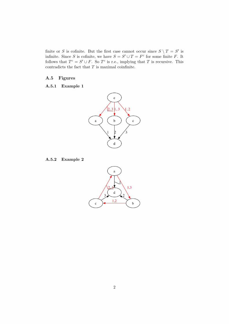
Each of Examples 1 and 2 below24 shows that the inclusion is sometimesstrict. Example 1 also shows that an alternative can be in the core even ifit is not maximal with respect to anyone’s preference:

Example 1 Let N = {1, 2, 3} and let W consist of the coalitions having amajority (i.e., having at least two players). Let X = {a, b, c, d, e}. Definea profile by �1= {(a, d), (e, b), (e, c)}, �2= {(b, d), (e, a), (e, c)}, and �3={(c, d), (e, a), (e, b)}. Then the sets max �i of maximal elements of X withrespect to �i are given by max �1= {a, e}, max �2= {b, e}, and max �3={c, e}. But the core C is {d, e}. So, the core is neither a subset nor a supersetof

∪i max �i= {a, b, c, e}. The core C+ without majority dissatisfaction is

{e}, which is a subset of∪

i max �i.

Example 2 also shows that the core, even if it is nonempty, does notnecessarily intersect the union of the maximal elements of individual prefer-ences:

Example 2 We modify the simplest voting paradox (a cycle involving threealternatives and three players) by adding an alternative d. Let N = {1, 2, 3}and let W consist of the coalitions having a majority. Let X = {a, b, c, d}.Define a profile by �1= {(a, b), (b, c), (a, d)}, �2= {(b, c), (c, a), (b, d)}, and�3= {(c, a), (a, b), (c, d)}. Then the core C is {d}. So it does not inter-sect

∪i max �i= {a, b, c}. The core C+ without majority dissatisfaction is

empty.

Unlike the core, the core without majority dissatisfaction is always in-cluded in the union of the maximal elements of individual preferences:

Lemma 6 For each profile p, we have C+(W, B,p) ⊆ C(W, B,p)∩(∪

i maxB �pi

).25

24See Appendix A.5 for graph representations of the profiles in these examples.25Appendix A.3 shows that the inclusion is strict for some profile.

12

Proof. By Lemma 5, it suffices to show that C+ is a subset of∪

i maxB �pi .

Suppose x ∈ B but x /∈∪

i maxB �pi . Then, x /∈ maxB �p

i for any i ∈ N .This implies that {i : x /∈ maxB �p

i } = N ⊇ S for any winning coalitionS ∈ W. (Such an S exists since W 6= ∅.) By the definition of C+, we havex /∈ C+.

4 Preferences with Maximal Alternatives

We consider in the rest of the paper profiles for a set B of alternatives, thatis, measurable profiles consisting of preferences that have a maximal elementof B.

4.1 The results for the core of a simple game

We now give a version of Nakamura’s theorem for profiles for a set B ofalternatives:

Theorem 2 Let W ⊆ B be a simple game and B ⊆ X an agenda. LetM(B)N

B be the set of measurable profiles of preferences having a maximalelement of B. Then the following statements are equivalent:26

(i) #B < ν(W);(ii) the core C+(W, B,p) without majority dissatisfaction is nonempty forall p ∈ M(B)N

B ;(iii) the core C(W, B,p) is nonempty for all p ∈ M(B)N

B .

Proof. (i)⇒(ii). Suppose C+(W, B,p) = ∅ for some profile p for B. ByDefinition 1, for each x ∈ B, there is a winning coalition Sx ∈ W such thatSx ⊆ {i : x /∈ max �p

i }. We claim that∩

x∈B Sx = ∅. (Otherwise, there isan i who is in Sx for all x ∈ B. It follows that �p

i has no maximal elementof B.) The claim shows that ν(W) ≤ #B.

(ii)⇒(iii). Immediate from Lemma 5.

(iii)⇒(i). Suppose #B ≥ ν(W). We construct a profile p for B suchthat C(W, B,p) = ∅. Let ν = ν(W) ≥ 2.

Step 1, Case (a): ν is finite. We construct a profile p such that thedominance relation �p

W has a cycle consisting of ν alternatives (and thecycle contains an alternative x0 greater than any alternative y not belongingto the cycle).

By the definition of the Nakamura number, there is a collection W ′ ={L0, . . . , Lν−1} of winning coalitions such that

∩W ′ =

∩ν−1k=0 Lk = ∅.

26 The implication (iii)⇒(ii) is not the same as the following statement (Example 2):for each p ∈ M(B)N

B , if C(W, B,p) 6= ∅, then C+(W, B,p) 6= ∅.

13

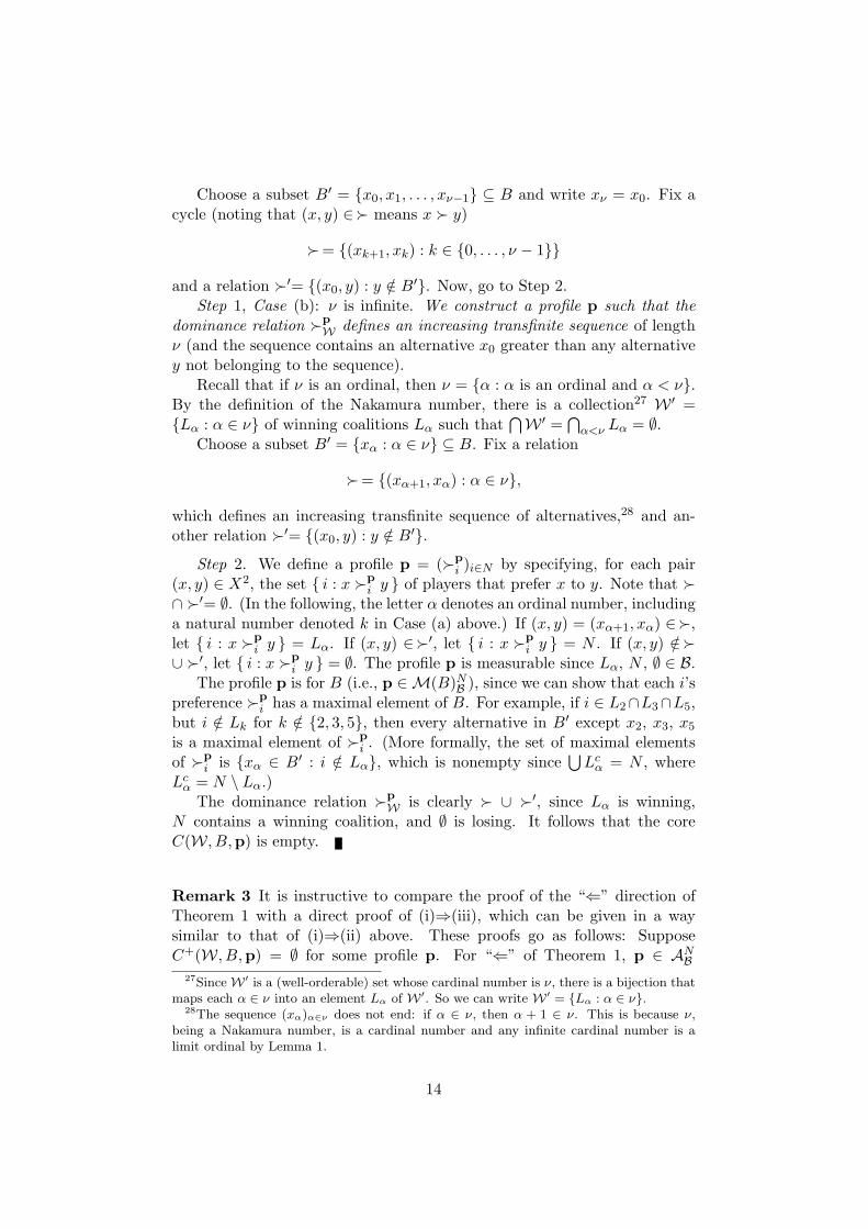
Choose a subset B′ = {x0, x1, . . . , xν−1} ⊆ B and write xν = x0. Fix acycle (noting that (x, y) ∈� means x � y)

�= {(xk+1, xk) : k ∈ {0, . . . , ν − 1}}

and a relation �′= {(x0, y) : y /∈ B′}. Now, go to Step 2.Step 1, Case (b): ν is infinite. We construct a profile p such that the

dominance relation �pW defines an increasing transfinite sequence of length

ν (and the sequence contains an alternative x0 greater than any alternativey not belonging to the sequence).

Recall that if ν is an ordinal, then ν = {α : α is an ordinal and α < ν}.By the definition of the Nakamura number, there is a collection27 W ′ ={Lα : α ∈ ν} of winning coalitions Lα such that

∩W ′ =

∩α<ν Lα = ∅.

Choose a subset B′ = {xα : α ∈ ν} ⊆ B. Fix a relation

�= {(xα+1, xα) : α ∈ ν},

which defines an increasing transfinite sequence of alternatives,28 and an-other relation �′= {(x0, y) : y /∈ B′}.

Step 2. We define a profile p = (�pi )i∈N by specifying, for each pair

(x, y) ∈ X2, the set { i : x �pi y } of players that prefer x to y. Note that �

∩ �′= ∅. (In the following, the letter α denotes an ordinal number, includinga natural number denoted k in Case (a) above.) If (x, y) = (xα+1, xα) ∈�,let { i : x �p

i y } = Lα. If (x, y) ∈�′, let { i : x �pi y } = N . If (x, y) /∈�

∪ �′, let { i : x �pi y } = ∅. The profile p is measurable since Lα, N , ∅ ∈ B.

The profile p is for B (i.e., p ∈ M(B)NB ), since we can show that each i’s

preference �pi has a maximal element of B. For example, if i ∈ L2∩L3∩L5,

but i /∈ Lk for k /∈ {2, 3, 5}, then every alternative in B′ except x2, x3, x5

is a maximal element of �pi . (More formally, the set of maximal elements

of �pi is {xα ∈ B′ : i /∈ Lα}, which is nonempty since

∪Lc

α = N , whereLc

α = N \ Lα.)The dominance relation �p

W is clearly � ∪ �′, since Lα is winning,N contains a winning coalition, and ∅ is losing. It follows that the coreC(W, B,p) is empty.

Remark 3 It is instructive to compare the proof of the “⇐” direction ofTheorem 1 with a direct proof of (i)⇒(iii), which can be given in a waysimilar to that of (i)⇒(ii) above. These proofs go as follows: SupposeC+(W, B,p) = ∅ for some profile p. For “⇐” of Theorem 1, p ∈ AN

B27Since W ′ is a (well-orderable) set whose cardinal number is ν, there is a bijection that

maps each α ∈ ν into an element Lα of W ′. So we can write W ′ = {Lα : α ∈ ν}.28The sequence (xα)α∈ν does not end: if α ∈ ν, then α + 1 ∈ ν. This is because ν,

being a Nakamura number, is a cardinal number and any infinite cardinal number is alimit ordinal by Lemma 1.

14

is a profile of acyclic preferences; for (i)⇒(iii), p ∈ M(B)NB is a profile of

preferences having a maximal element (of B). Then,(a) for each x ∈ B, there are y ∈ B and a winning coalition Sx ∈ W suchthat Sx ⊆ {i : y �p

i x} (hence y �pW x).

Note that x is not a maximal element for the players in Sx. The desiredconclusion ν(W) ≤ #B follows if we show

∩x∈B Sx = ∅. So suppose there

is an i who is in Sx for all x ∈ B.

• To show “⇐” of Theorem 1, assume B is finite. By repeated applica-tion of (a), we find the dominance ≺p

W contains an infinitely ascendingsequence: x0 ≺ x1 ≺ x2 ≺ x3 ≺ · · ·. Since B is finite, the sequencecontains a cycle such as x2 ≺ x3 ≺ x4 ≺ x2 ≺ x3 ≺ · · ·. It follows thati’s preference contains the same cycle, which violates the assumption.

• For (i)⇒(iii) of Theorem 2, a contradiction is immediate: let x ∈ Bbe a maximal element for �p

i ; then i ∈ Sx is violated. We do not evenneed the assumption that B is finite. We remark that the possibilityremains that i ∈ Sx if x ∈ B is not a maximal element for i. So i’spreference may contain a cycle without contradiction; it consists onlyof non-maximal elements for her.

The following example is an application of Theorem 2. It gives a condi-tion for an infinite set of alternatives to have an element in the core, thatis, a maximal element with respect to the dominance relation �p

W .

Example 3 Let N = [0, 1] be the unit interval on the set of real numbersand let B consist of all subsets of N . Define a simple game W by S ∈W if and only if Sc is countable. Then, it is easy to show that ν(W)is uncountable. Let X be a countable set of alternatives (e.g., the set ofrational numbers in [0, 1]). Suppose that for each i, her preference �p

i hasa maximal alternative (e.g., a utility function representing �p

i has finitelymany “peaks,” all corresponding to rational numbers). Then, Theorem 2implies that C+(W, X,p) and C(W, X,p) both contain alternatives.

The profiles constructed in the proof of (iii)⇒(i) of Theorem 2 consistof individual preferences that may have more than one maximal alterna-tive. However, we can modify the proof in such a way that each individualpreference has exactly one maximal alternative. That gives the followingproposition:

Proposition 1 Let W ⊆ B be a simple game and B ⊆ X an agenda. Thenthe three equivalent statements (i), (ii), and (iii) in Theorem 2 are equivalentto the following statements:(ii.a) The core C+(W, B,p) without majority dissatisfaction is nonempty forall measurable profiles p of preferences having exactly one maximal elementof B.

15

(ii.b) The core C+(W, B,p) without majority dissatisfaction is nonempty forall measurable profiles p of linear orders having a maximal element of B.(iii.a) The core C(W, B,p) is nonempty for all measurable profiles p ofpreferences having exactly one maximal element of B.(iii.b) The core C(W, B,p) is nonempty for all measurable profiles p oflinear orders having a maximal element of B.

Proof. (ii)⇒(ii.a)⇒(ii.b) and (iii)⇒(iii.a)⇒(iii.b) are obvious. (ii.b)⇒(iii.b)is immediate from Lemma 5.

(iii.b)⇒(i). Suppose #B ≥ ν(W). We construct a profile p satisfyingthe condition such that C(W, B,p) = ∅. Let ν = ν(W) ≥ 2. In Step 1 ofthe proof of Theorem 2, replace the relation �′ by an arbitrary asymmetricsubrelation �′⊂ X × (X \ B′) that is linear on X \ B′ and satisfies x �′ ywhenever x ∈ B′ and y ∈ X \ B′. We replace Step 2 of the proof by thefollowing argument.

Case: ν is finite. Define L−1 = N and for all k ∈ {0, . . . , ν − 1},

Dk = (L−1 ∩ L0 ∩ · · · ∩ Lk−1) \ Lk.

Then {D0, . . . , Dν−1} is a family of (possibly empty) pairwise disjoint coali-tions in B such that Lk ⊆ Dc

k := N \ Dk for all k and∪ν−1

k=0 Dk = N (i ∈ Nis in the first Dk such that i /∈ Lk).

Define p as follows: for each k, all players i in Dk have the same linearlyordered preference �p

i with maximal element xk, obtained by taking thetransitive closure of � \{(xk+1, xk)}∪ �′. Obviously, p is measurable sincefor each x, y ∈ X, { i : x �p

i y } is a finite union of Dk’s. Also, �pW includes

� ∪ �′. (If (x, y) = (xk+1, xk) ∈�, we have { i : x �pi y } = Dc

k ⊇ Lk ∈ W ′.If (x, y) ∈�′, then { i : x �p

i y } = N .) It follows that C(W, X,p) = ∅.

Case: ν is infinite. Note that (B′ × B′)∩ �′= ∅. Define p as follows:If (x, y) ∈�′, then { i : x �p

i y } = N . If (x, y) /∈ (B′ × B′)∪ �′, then{ i : x �p

i y } = ∅. If (x, y) = (xα, xβ) ∈ B′ × B′, xα �pi xβ if and only if

either29

• i ∈ Lcα ∩ Lc

β and α < β; or

• i ∈ Lcα ∩ Lβ and α 6= β; or

• i ∈ Lα ∩ Lβ and α > β.

29For each i, {xα : i ∈ Lcα} 6= ∅ is i’s preferred class of alternatives in B′ and {xα : i ∈

Lα} is her less-preferred class. Her preference �pi is linear on B′ satisfying the following

conditions: (a) if two alternatives belong to her preferred class, then i prefers the one withthe smaller index; (b) i prefers each alternative in her preferred class to any in her less-preferred class; (c) if two alternatives belong to her less-preferred class, then i prefers theone with the greater index. For example, if i ∈ L2 ∩ L3 ∩ L5, but i /∈ Lα for α /∈ {2, 3, 5},then i ranks the alternatives in the following order: x0, x1, x4, x6, x7, . . . , x5, x3, x2.

16

This is equivalent to saying that 30

{ i : x �pi y } = {i : xα �p

i xβ} =

Lc

α if α < β,Lβ if α > β,∅ if α = β.

The profile p is measurable since N , ∅, Lcα, Lβ ∈ B.

Clearly, each i’s preference �pi is a linear order on X that has a unique

maximal element of B, namely the alternative in her preferred class {xα :i ∈ Lc

α} 6= ∅ with the smallest index.The dominance relation �p

W clearly includes � ∪ �′, since {i : xβ+1 �pi

xβ} = Lβ ∈ W for each β ∈ ν, for example. It follows that C(W, X,p) =∅.

Remark 4 The argument for the finite ν case of the proof does not gothrough for the infinite case, since Dk does not necessarily belong to Bwhen k is infinite. The argument for the infinite case causes difficulty whenapplied to the finite case. For example, suppose ν = 4 and i ∈ L0 ∩ L3.Since i ∈ L3 and 4 > 3, we have x4 �p

i x3 by the definition of p. Sincei ∈ L0 and 3 > 0, we have x3 �p

i x0. Since x0 = x4, �pi is not asymmetric.

4.2 The results for the core of a collection of winning sets

4.2.1 Extended framework

We extend the framework by introducing a collection B′, consisting of subsetsof the set N of players. Recall that B consists of the coalitions—intuitively,they are the observable or identifiable sets of players. In contrast, B′ consistsof the sets for which one can assign winning/losing status—sometimes theyare the sets whose size is well-defined (Example 4); other times they are thesets that are half-identifiable or listable (Example 5). We assume B ⊆ B′,which means that one can assign such a status for any coalition.

A collection W ′ of winning sets is a subcollection of B′ satisfying∅ /∈ W ′ and W ′ 6= ∅. Given W ′, the most natural simple game one candefine is the following: the B-simple game W induced by W ′ consists ofthe winning coalitions (winning sets that are also coalitions), that is, W =W ′∩B. We can define the core and the core without majority dissatisfactionas before, with W replaced by W ′. Lemma 5 and W ⊆ W ′ imply thefollowing.

Lemma 7 Let W ′ ⊆ B′ and W = W ′ ∩ B. Then the following statementsare true:

30xα �pi xβ iff either (1) α < β and i ∈ (Lc

α ∩ Lcβ) ∪ (Lc

α ∩ Lβ) = Lcα ∩ (Lc

β ∪ Lβ) = Lcα

or (2) α > β and i ∈ (Lcα ∩ Lβ) ∪ (Lα ∩ Lβ) = Lβ . Note that the first two cases can be

restated: if α < β, then {i : xβ �pi xα} = Lα and {i : xα �p

i xβ} = Lcα.

17

(i) C+(W ′, B,p) ⊆ C+(W, B,p) ⊆ C(W, B,p).(ii) C+(W ′, B,p) ⊆ C(W ′, B,p) ⊆ C(W, B,p).

Since we had better be able to identify who prefers a given alternativeto another, we leave the definitions of measurable profiles and profiles foran agenda unaltered.

4.2.2 Justification for the extended framework

We have assumed B′ = B in the previous sections, but there are reasonsfor distinguishing the collection B′ from the Boolean algebra B of coalitions.We illustrate that by two examples in this section. We also give an exampleof a decision-making situation where the framework makes sense.

The following example gives some, though limited, justification for theextended framework:

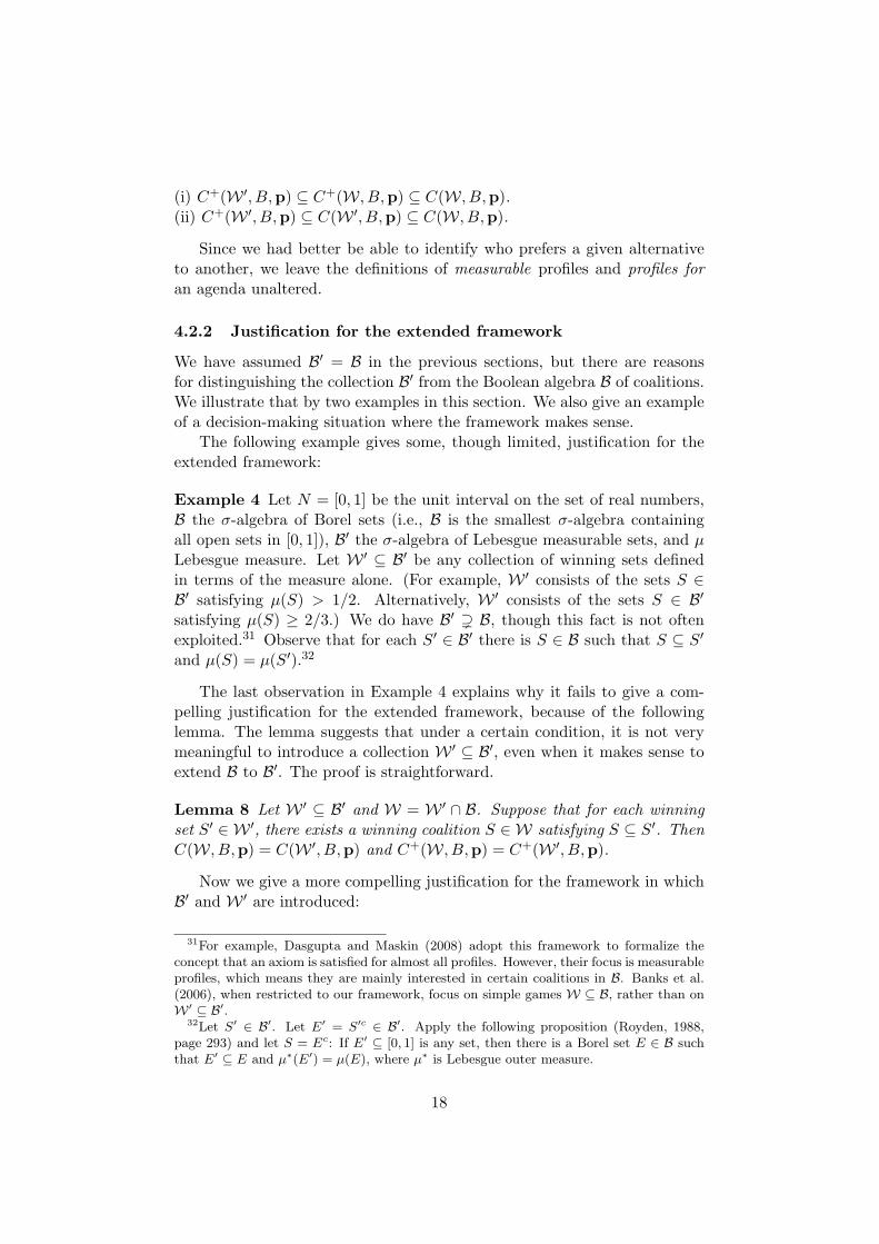
Example 4 Let N = [0, 1] be the unit interval on the set of real numbers,B the σ-algebra of Borel sets (i.e., B is the smallest σ-algebra containingall open sets in [0, 1]), B′ the σ-algebra of Lebesgue measurable sets, and µLebesgue measure. Let W ′ ⊆ B′ be any collection of winning sets definedin terms of the measure alone. (For example, W ′ consists of the sets S ∈B′ satisfying µ(S) > 1/2. Alternatively, W ′ consists of the sets S ∈ B′

satisfying µ(S) ≥ 2/3.) We do have B′ ) B, though this fact is not oftenexploited.31 Observe that for each S′ ∈ B′ there is S ∈ B such that S ⊆ S′

and µ(S) = µ(S′).32

The last observation in Example 4 explains why it fails to give a com-pelling justification for the extended framework, because of the followinglemma. The lemma suggests that under a certain condition, it is not verymeaningful to introduce a collection W ′ ⊆ B′, even when it makes sense toextend B to B′. The proof is straightforward.

Lemma 8 Let W ′ ⊆ B′ and W = W ′ ∩ B. Suppose that for each winningset S′ ∈ W ′, there exists a winning coalition S ∈ W satisfying S ⊆ S′. ThenC(W, B,p) = C(W ′, B,p) and C+(W, B,p) = C+(W ′, B,p).

Now we give a more compelling justification for the framework in whichB′ and W ′ are introduced:

31For example, Dasgupta and Maskin (2008) adopt this framework to formalize theconcept that an axiom is satisfied for almost all profiles. However, their focus is measurableprofiles, which means they are mainly interested in certain coalitions in B. Banks et al.(2006), when restricted to our framework, focus on simple games W ⊆ B, rather than onW ′ ⊆ B′.

32Let S′ ∈ B′. Let E′ = S′c ∈ B′. Apply the following proposition (Royden, 1988,page 293) and let S = Ec: If E′ ⊆ [0, 1] is any set, then there is a Borel set E ∈ B suchthat E′ ⊆ E and µ∗(E′) = µ(E), where µ∗ is Lebesgue outer measure.

18

Example 5 Let N = {0, 1, 2, . . .} be the set of natural numbers. A naturaland faithful way to model identifiable or half-identifiable sets of players isto let B be the algebra of recursive sets (coalitions) and B′ the lattice of r.e.sets.33

The first reason for introducing B′ ⊇ B in our framework is that wecannot let B be the lattice of r.e. sets, since the lattice is not a Booleanalgebra.

The second reason is that the natural system (We)e∈N for indexing r.e.sets is easier to handle than the system (ϕe)e∈N that can be used for indexingrecursive sets (where ϕe is the eth partial recursive function and We itsdomain). For example, while ϕe corresponds to (i.e., is the characteristicfunction of) no recursive set for some e ∈ N (and there is no algorithm todecide whether a given e corresponds to some recursive set), We correspondsto (i.e., is) an r.e. set for any e ∈ N . One can therefore write any class of r.e.sets as {We : e ∈ I} for some (not necessarily r.e.) set I of indices, withoutworrying that some We might correspond to no r.e. set. Odifreddi (1992,page 226) gives more reasons for preferring (We)e∈N to (ϕe)e∈N .

We now give a reason for introducing W ′ ⊆ B′ into our framework. Weexhibit W ′, W = W ′ ∩ B, and p for which C+(W, X,p) 6= C+(W ′, X,p).

A set is cofinite if it is the complement of a finite set; otherwise, it iscoinfinite. A coinfinite r.e. set T is maximal coinfinite34 if it has onlytrivial supersets: if S is a coinfinite r.e. set satisfying S ⊇ T , then S \ T isfinite.

Let W ′0 be the collection of all maximal coinfinite sets. Since maximal

coinfinite sets are nonrecursive, we have W0 = W ′0 ∩ B = ∅, which is not

a simple game according to our definition. We can nevertheless concludeW0 6= W ′

0 and define the core, obtaining C(W0, X,p) = C+(W0, X,p) = Xfor any profile p. Let X = {a, b, c} and define a profile p by �p

i = {(a, b)}for all i ∈ N . Then, C(W ′

0, X,p) = C+(W ′0, X,p) = {a, c} 6= X.

Let W ′1 = {S′ ∈ B′ : S′ ⊇ T for some maximal coinfinite T}. Then we

can easily show that W1 = W ′1 ∩ B consists of all cofinite sets; therefore,

W1 6= W ′1. Let X = {x−1, x0, x1, x2, . . .} be a countable set. Let T ∈ B′

be a maximal coinfinite set. Define a profile p as follows: �pi = {(xi, x−1)}

if i ∈ T ; �pi = ∅ otherwise. Then, { i : x �p

i y } is {i} if x = xi for i ∈ T

33According to Church’s thesis (Odifreddi, 1992), a set of players (natural numbers) isrecursive if there is an algorithm that, given any player, will decide whether she is in theset. A set of players is r.e. (recursively enumerable) if there is an algorithm that lists, insome order, the members of the set; the condition in general does not mean that there isan algorithm to decide whether a given player belongs to it. A set A ⊆ N is recursive ifand only if A and Ac are both r.e. Odifreddi (1992) gives detailed discussion of recursiontheory (computability theory). The papers by Mihara (1997, 1999) contain short reviewsof recursion theory.

34What we call maximal coinfinite sets are known as maximal sets in recursion theory(Odifreddi, 1992, page 288). Friedberg (1958) constructively proves the existence of suchsets.

19

and y = x−1; it is ∅ otherwise. So p is measurable and each player hasa maximal alternative. We have C(W1, X,p) = C(W ′

1, X,p) = X. Also,{i : x /∈ max �p

i } is T if x = x−1; it is ∅ otherwise. So, C+(W1, X,p) = Xbut C+(W ′

1, X,p) = X \ {x−1}.

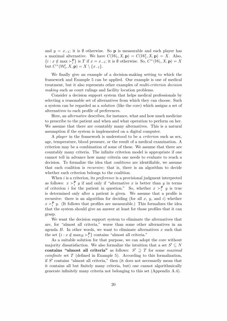
We finally give an example of a decision-making setting to which theframework and Example 5 can be applied. Our example is one of medicaltreatment, but it also represents other examples of multi-criterion decisionmaking such as court rulings and facility location problems.

Consider a decision support system that helps medical professionals byselecting a reasonable set of alternatives from which they can choose. Sucha system can be regarded as a solution (like the core) which assigns a set ofalternatives to each profile of preferences.

Here, an alternative describes, for instance, what and how much medicineto prescribe to the patient and when and what operation to perform on her.We assume that there are countably many alternatives. This is a naturalassumption if the system is implemented on a digital computer.

A player in the framework is understood to be a criterion such as sex,age, temperature, blood pressure, or the result of a medical examination. Acriterion may be a combination of some of these. We assume that there arecountably many criteria. The infinite criterion model is appropriate if onecannot tell in advance how many criteria one needs to evaluate to reach adecision. To formalize the idea that coalitions are identifiable, we assumethat each coalition is recursive; that is, there is an algorithm to decidewhether each criterion belongs to the coalition.

When i is a criterion, its preference is a provisional judgment interpretedas follows: x �p

i y if and only if “alternative x is better than y in termsof criterion i for the patient in question.” So, whether x �p

i y is trueis determined only after a patient is given. We assume that a profile isrecursive: there is an algorithm for deciding (for all x, y, and i) whetherx �p

i y. (It follows that profiles are measurable.) This formalizes the ideathat the system should give an answer at least for those profiles that it cangrasp.

We want the decision support system to eliminate the alternatives thatare, for “almost all criteria,” worse than some other alternatives in anagenda B. In other words, we want to eliminate alternatives x such thatthe set {i : x /∈ maxB �p

i } contains “almost all criteria.”As a suitable solution for that purpose, we can adopt the core without

majority dissatisfaction. We also formalize the intuition that a set S′ ⊆ Ncontains “almost all criteria” as follows: S′ ⊇ T for some maximalcoinfinite set T (defined in Example 5). According to this formalization,if S′ contains “almost all criteria,” then (it does not necessarily mean thatit contains all but finitely many criteria, but) one cannot algorithmicallygenerate infinitely many criteria not belonging to this set (Appendix A.4).

20

Suppose, for the time being, that one can assign winning/losing statusonly to (recursive) coalitions. One can naturally define that a coalition Sis winning if it contains “almost all criteria”; that is, S ⊇ T for somemaximal coinfinite T . A problem is that the set {i : x /∈ maxB �p

i } may(i) contain “almost all criteria” without (ii) containing a winning coalition.That is, we want to eliminate x, but the definition (Definition 1) of the corewithout majority dissatisfaction does not allow us to eliminate it. Indeed,Example 5 shows that when the set itself is maximal coinfinite, it containsno winning coalition.

To rectify this problem, we assign winning/losing status to every r.e.set of criteria. (An r.e. set is half-identifiable in the sense that there isan algorithm that enumerates its elements.) We define that an r.e. setis winning if it contains “almost all criteria” as above. We then havethe equivalence of the following for r.e. sets S′: (i) S′ contains “almost allcriteria”; (ii) S′ contains a winning r.e. set; (iii) S′ is winning. Fortunately,when B is r.e., the set {i : x /∈ maxB �p

i } is also r.e., since it can be rewrittenas {i : ∃y[y ∈ B ∧ y �p

i x]}. So to determine whether to reject x here, weonly need to check whether this set is winning.

4.2.3 The results for the extended framework

Before stating the main result for the extended framework, we need to extendthe notion of the Nakamura number.

Let B′ ⊇ B be a collection that includes B, the Boolean algebra of coali-tions. Let W ′ ⊆ B′ be a collection of winning sets. A nonempty collectionZ ⊆ B is a (B)-cover of S′ ∈ B′ if

∪Z :=

∪S∈Z S ⊇ S′. If Z is a finite cover,

then∪

Z ∈ B, since B is a Boolean algebra. So, we can assume without lossof generality that #Z is either 1 or infinite. Let M(W ′) be the collection ofpairs (Y,Z) such that(a) Y ⊆ W ′ and(b) Z:Y →→ B is a correspondence that maps each winning set W ∈ Y toa B-cover Z(W ) of W and that satisfies

∩W∈Y

∪Z(W ) = ∅.

Definition 2 The kappa number κ(W ′) of a collection W ′ of winningsets relative to B is +∞ (greater than any cardinal number) if M(W ′) = ∅;otherwise, it is the cardinal number given by35

κ(W ′) = min(Y,Z)∈M(W ′)

max{#Y, sup{#Z(W ) : W ∈ Y}}.

35The right-hand side is well-defined, since every set of ordinals has a supremum(Hrbacek and Jech, 1984, page 141) as well as the least element. (The same is not true forclasses that are not sets, like the class of all cardinal numbers.) To see the supremum is acardinal number, let supγ αγ = α, where each αγ is a cardinal number. It suffices to showthat α is an initial ordinal. Suppose β < α. Then, by the definition of the supremum,β < αγ for some γ. Since αγ is a cardinal, #β < αγ . But αγ ≤ α implies that α is notequipotent to β.

21

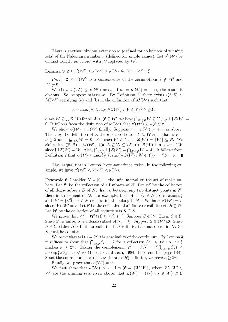
There is another, obvious extension ν ′ (defined for collections of winningsets) of the Nakamura number ν (defined for simple games). Let ν ′(W ′) bedefined exactly as before, with W replaced by W ′.

Lemma 9 2 ≤ ν ′(W ′) ≤ κ(W ′) ≤ ν(W) for W = W ′ ∩ B.

Proof. 2 ≤ ν ′(W ′) is a consequence of the assumptions ∅ /∈ W ′ andW ′ 6= ∅.

We show ν ′(W ′) ≤ κ(W ′) next. If κ := κ(W ′) = +∞, the result isobvious. So, suppose otherwise. By Definition 2, there exists (Y,Z) ∈M(W ′) satisfying (a) and (b) in the definition of M(W ′) such that

κ = max{#Y, sup{#Z(W ) : W ∈ Y}} ≥ #Y.

Since W ⊆∪

Z(W ) for all W ∈ Y ⊆ W ′, we have∩

W∈Y W ⊆∩

W∈Y

∪Z(W ) =

∅. It follows from the definition of ν ′(W ′) that ν ′(W ′) ≤ #Y ≤ κ.We show κ(W ′) ≤ ν(W) finally. Suppose ν := ν(W) 6= +∞ as above.

Then, by the definition of ν, there is a collection Y ⊆ W such that #Y =ν ≥ 2 and

∩W∈Y W = ∅. For each W ∈ Y, let Z(W ) = {W} ⊆ B. We

claim that (Y,Z) ∈ M(W ′). ((a) Y ⊆ W ⊆ W ′. (b) Z(W ) is a cover of Wsince

∪Z(W ) = W . Also,

∩W∈Y

∪Z(W ) =

∩W∈Y W = ∅.) It follows from

Definition 2 that κ(W ′) ≤ max{#Y, sup{#Z(W ) : W ∈ Y}} = #Y = ν.

The inequalities in Lemma 9 are sometimes strict. In the following ex-ample, we have ν ′(W ′) < κ(W ′) < ν(W).

Example 6 Consider N = [0, 1], the unit interval on the set of real num-bers. Let B′ be the collection of all subsets of N . Let W ′ be the collectionof all dense subsets D of N , that is, between any two distinct points in N ,there is an element of D. For example, both W = {r ∈ N : r is rational}and W ′ = {

√2 + r ∈ N : r is rational} belong to W ′. We have ν ′(W ′) = 2,

since W ∩W ′ = ∅. Let B be the collection of all finite or cofinite sets S ⊆ N .Let W be the collection of all cofinite sets S ⊆ N .

We prove that W = W ′ ∩ B ( W ′. (⊆): Suppose S ∈ W. Then, S ∈ B.Since Sc is finite, S is a dense subset of N . (⊇): Suppose S ∈ W ′∩B. SinceS ∈ B, either S is finite or cofinite. If S is finite, it is not dense in N . SoS must be cofinite.

We prove that ν(W) = 2ω, the cardinality of the continuum. By Lemma 3,it suffices to show that

∩α<ν Sα = ∅ for a collection {Sα ∈ W : α < ν}

implies ν ≥ 2ω. Taking the complement, 2ω = #N = #(∪

α<ν Scα) ≤

ν · sup{#Scα : α < ν} (Hrbacek and Jech, 1984, Theorem 1.3, page 188).

Since the supremum is at most ω (because Scα is finite), we have ν ≥ 2ω.

Finally, we prove that κ(W ′) = ω.We first show that κ(W ′) ≤ ω. Let Y = {W,W ′}, where W , W ′ ∈

W ′ are the winning sets given above. Let Z(W ) = {{r} : r ∈ W} ⊂ B

22

and Z(W ′) = {{r′} : r′ ∈ W ′} ⊂ B. It is straightforward to show that(Y,Z) ∈ M(W ′). Since #Y = 2 and sup{#Z(W ), #Z(W ′)} = ω, we haveκ(W ′) ≤ ω.

We next show that κ(W ′) is not finite. Suppose it is finite. Then, thereexists (Y,Z) ∈ M(W ′) such that Y is finite and Z(W ) ⊂ B is finite for eachW ∈ Y. Since B is a Boolean algebra, this implies that

∪Z(W ) ∈ B, which

in turn implies that∪

Z(W ) is either finite or cofinite. Suppose∪

Z(W ) isfinite for some W ∈ Y ⊆ W ′. Then

∪Z(W ) ⊇ W implies that W ∈ W ′ is

finite, a contradiction. Hence∪

Z(W ) is cofinite for all W ∈ Y. Being afinite intersection of cofinite sets,

∩W∈Y

∪Z(W ) is nonempty, contrary to

assumption.

Lemma 10 κ is an extension of ν. That is, if W ′ ⊆ B ⊆ B′, then κ(W ′) =ν(W ′).

Proof. Suppose W ′ ⊆ B. Then, W = W ′ ∩ B = W ′. Lemma 9 impliesν ′(W ′) ≤ κ(W ′) ≤ ν(W ′). Since ν ′ extends ν and W ′ is a simple game inthis case, we have ν ′(W ′) = ν(W ′), from which the conclusion follows.

We now give the main result for the extended framework.

Theorem 3 Let W ′ ⊆ B′ be a collection of winning sets and B ⊆ X anagenda. Let M(B)N

B be the set of measurable profiles of preferences havinga maximal element of B. Then the following two statements are equivalent:(i) #B < κ(W ′);(ii) the core C+(W ′, B,p) without majority dissatisfaction is nonempty forall p ∈ M(B)N

B .Moreover, these equivalent statements imply, but are not implied by(iii) the core C(W ′, B,p) is nonempty for all p ∈ M(B)N

B .

Proof.36 (i)⇒(ii). Suppose C+(W ′, B,p) = ∅ for some profile p ∈M(B)N

B . We show that #B ≥ κ(W ′).By the definition (Definition 1) of C+, for each x ∈ B, there is a winning

set Wx ∈ W ′ such that Wx ⊆ { i : x /∈ maxB �pi }. We claim that

∩x∈B{ i :

x /∈ maxB �pi } = ∅. (Otherwise, there is a player i whose preference has no

maximal element of B.)Let Y = {Wx : x ∈ B} ⊆ W ′. We have #Y ≤ #B. For each Wx ∈ Y,

letZ(Wx) = {{ i : y �p

i x } : y ∈ B}.

We have #Z(Wx) ≤ #B.We claim that (Y,Z) ∈ M(W ′). (Details. We verify (b) of the definition

of M(W ′). First, Z(Wx) ⊆ B since p measurable implies { i : y �pi x } ∈ B.

Second, Z(Wx) is a cover of Wx since∪

Z(Wx) =∪

y∈B{ i : y �pi x } = { i :

36Lemmas 7 and 9 are not useful for proving Theorem 3 from Theorem 2, and vice versa.

23

x /∈ maxB �pi } ⊇ Wx. Third,

∩Wx∈Y

∪Z(Wx) =

∩x∈B{ i : x /∈ maxB �p

i

} = ∅ by the claim above.)By the definition (Definition 2) of κ, we get

κ(W ′) ≤ max{#Y, sup{#Z(Wx) : x ∈ B}} ≤ #B.

(ii)⇒(i). Suppose #B ≥ κ := κ(W ′). We construct a profile p ∈M(B)N

B such that C+(W ′, B,p) = ∅. By the definition (Definition 2) ofκ(·), there exists (Y,Z) ∈ M(W ′) such that37

(a) Y = {Lα : α < κ′} ⊆ W ′, where κ′ := #Y:(b) Z maps each Lα ∈ Y to Z(Lα) = {Lβ

α : β < β(α)} ⊆ B (whereβ(α) := #Z(Lα)) satisfying L′

α :=∪

Z(Lα) =∪

β<β(α) Lβα ⊇ Lα ∈ W ′

and∩

Lα∈Y∪

Z(Lα) =∩

α<κ′ L′α = ∅;

(c) κ = max{κ′, sup{β(α) : α < κ′}} ≤ #B.Write B = {xα : α < #B} and let B′ = {xα : α < κ′}.

Case: κ is finite. We construct a profile p such that the dominancerelation �p

W has a cycle consisting of κ alternatives. Since β(α) ≤ κ is finitefor all α < κ′ in this case, L′

α =∪

β Lβα is a finite union of elements of the

Boolean algebra B. So we can assume L′α ∈ B and β(α) = 1 without loss

of generality. By (c), we have κ′ = κ. Write xκ = x0 and fix a relation�′= {(x0, y) : y /∈ B′}. Let

�pi = {(xα+1, xα) : L′

α 3 i}∪ �′

for all i ∈ N . The profile p is the same as that in the proof of Theorem 2,except that Lα is replaced by L′

α ∈ B. The rest of the proof runs as before.

Case: κ is infinite. We construct a profile p such that for each alternativexα ∈ B, there is a winning set of players i who prefer another alternativexα+βi

∈ B to xα.38 Since preferences involving alternatives outside B areirrelevant, we construct the profile in such a way that it satisfies �p

i ⊆ B×Bfor all i.

We define p by specifying { i : x �pi y } for each pair (x, y) = (xα′ , xα) ∈

B×B satisfying α′ > α. (If (x, y) does not satisfy the conditions concerningthe indices, then { i : x �p

i y } = ∅.) Note that each such pair can beuniquely written as (x, y) = (xα+β , xα) for some β > 0.39 Let L1

α = ∅if β(α) = 1; otherwise, we can assume β(α) is infinite. Define p by the

37We can write Y and Z(Lα) in the form below (footnote 27).38Though not required in our setting, we construct the profile so that individual pref-

erences will be acyclic. This is achieved by the following: no player prefers an alternativexα′ ∈ B with smaller index to xα (if α′ ≤ α, then xα′ 6�p

i xα).39β is the unique ordinal isomorphic to {γ : α ≤ γ < α′}.

24

following, which immediately establishes that p is measurable:40

{i : xα+β �pi xα} =

L0

α ∪ L1α ∈ B if α < κ′ and β = 1,

Lβα ∈ B if α < κ′ and 1 < β < β(α),

N ∈ B if κ′ ≤ α < #B and β = 1,∅ ∈ B otherwise.

For each xα ∈ B, we have {i : xα /∈ maxB �pi } =

∪β{i : xα+β �p

i

xα}, which equals∪

β<β(α) Lβα = L′

α (if α < κ′; the equality holds whetherβ(α) is 1 or infinite) or N (otherwise). In either case, the set contains awinning set Lα ∈ W ′. Therefore, xα /∈ C+(W ′, B,p). This establishes thatC+(W ′, B,p) = ∅.

To establish that p ∈ M(B)NB , we need to show that each i’s pref-

erence �pi has a maximal element of B. Since

∩α<κ′ L′

α = ∅, we have∪α<κ′(L′

α)c = N . So, for each i ∈ N , there is an α < κ′ such that i /∈ L′α.

Since i /∈ Lβα for any β < β(α), we have xα ∈ maxB �p

i by the definitionof p.

(ii)⇒(iii). Immediate from Lemma 7.

(iii)6⇒(i). Consider Example 6. We first prove that C(W ′, B,p) =C(W, B,p) for all p ∈ M(B)N

B and all B ⊆ X. By Lemma 7, it suffices toshow that C(W, B,p) ⊆ C(W ′, B,p). Suppose x ∈ B is not in C(W ′, B,p).Then, there are y ∈ B and S ∈ W ′ such that S ⊆ { i : y �p

i x }. Since p ismeasurable, { i : y �p

i x } ∈ B is either finite or cofinite. If it is finite, thenS ∈ W ′ is finite, a contradiction. It follows that { i : y �p

i x } is cofinite,hence it belongs to W. So x /∈ C(W, B,p).

Choose an agenda B satisfying #B = ω. (i) is violated since #B = ω 6<ω = κ(W ′). On the other hand, since #B = ω < 2ω = ν(W), Theorem 2implies that C(W, B,p) 6= ∅ for all p ∈ M(B)N

B . Then (iii) is satisfied sinceC(W ′, B,p) = C(W, B,p).

References

Ambrus, A., Rozen, K., Jul. 2008. Revealed conflicting preferences. Discus-sion Paper 1670, Cowles Foundation, Yale University, New Haven.40See Appendix A.5 for a graph representation of the profile. For the subsequent argu-

ment, we need to verify that xα+β and xα corresponding to the first two cases do existin B, that is, α + β < #B (and α < #B, which is obvious). For the first and the thirdcases, since α < #B, we have α+β = α+1 < #B. This is because #B, being an infinitecardinal number, is a limit ordinal by Lemma 1. For the second case, since α < κ′ ≤ #B,we have #α < #B. This is because #B, being a cardinal number, is not equipotent toα < #B. Similarly, since β < β(α) ≤ #B, we have #β < #B. If α and β are finite,the conclusion is obvious since #B is infinite in this case. Suppose otherwise. Then, byLemma 2, we have #(α + β) = #α + #β = max{#α, #β} < #B = #(#B). This impliesthat there is no one-to-one function from #B to α + β. Therefore, α + β < #B.

25

Andjiga, N. G., Mbih, B., 2000. A note on the core of voting games. Journalof Mathematical Economics 33, 367–372.

Andjiga, N. G., Moulen, J., 1989. Necessary and sufficient conditions forl-stability of games in constitutional form. International Journal of GameTheory 18, 91–110.

Andjiga, N. G., Moyouwou, I., 2006. A note on the non-emptiness of thestability set when individual preferences are weak orders. MathematicalSocial Sciences 52, 67–76.

Arrow, K. J., 1963. Social Choice and Individual Values, 2nd Edition. YaleUniversity Press, New Haven.

Austen-Smith, D., Banks, J. S., 1999. Positive Political Theory I: CollectivePreference. University of Michigan Press, Ann Arbor.

Banks, J. S., 1985. Sophisticated voting outcomes and agenda control. SocialChoice and Welfare 1, 295–306.

Banks, J. S., 1995. Acyclic social choice from finite sets. Social Choice andWelfare 12, 293–310.

Banks, J. S., Duggan, J., Le Breton, M., 2006. Social choice and electoralcompetition in the general spatial model. Journal of Economic Theory126, 194–234.

Dasgupta, P., Maskin, E., 2008. On the robustness of majority rule. Journalof the European Economic Association 6, 949–973.

Duggan, J., 2007. A systematic approach to the construction of non-emptychoice sets. Social Choice and Welfare 28, 491–506.

Fishburn, P. C., 1970. Arrow’s Impossibility Theorem: Concise proof andinfinite voters. Journal of Economic Theory 2, 103–6.

Friedberg, R. M., 1958. Three theorems on recursive enumeration. I. decom-position, II. maximal set, III. enumeration without duplication. Journalof Symbolic Logic 23, 309–316.

Hrbacek, K., Jech, T., 1984. Introduction to Set Theory, second, revised andexpanded edition. Marcel Dekker, New York.

Kalai, G., Rubinstein, A., Spiegler, R., 2002. Rationalizing choice functionsby multiple rationales. Econometrica 70, 2481–2488.

Kreps, D. M., 1979. A representation theorem for “preference for flexibility”.Econometrica 47, 565–577.

26

Kumabe, M., Mihara, H. R., 2008a. Computability of simple games: Acharacterization and application to the core. Journal of MathematicalEconomics 44, 348–366.

Kumabe, M., Mihara, H. R., 2008b. The Nakamura numbers for computablesimple games. Social Choice and Welfare 31, 621–640.

Le Breton, M., Salles, M., 1990. The stability set of voting games: Classi-fication and genericity results. International Journal of Game Theory 19,111–127.

Lipman, B. L., 1991. How to decide how to decide how to . . . : Modelinglimited rationality. Econometrica 59, 1105–1125.

Martin, M., Merlin, V., 2006. On the characteristic numbers of voting games.International Game Theory Review 8, 643–654.

Mihara, H. R., 1997. Arrow’s Theorem and Turing computability. EconomicTheory 10, 257–76.

Mihara, H. R., 1999. Arrow’s theorem, countably many agents, and morevisible invisible dictators. Journal of Mathematical Economics 32, 267–287.

Mihara, H. R., 2000. Coalitionally strategyproof functions depend only onthe most-preferred alternatives. Social Choice and Welfare 17, 393–402.

Nakamura, K., 1979. The vetoers in a simple game with ordinal preferences.International Journal of Game Theory 8, 55–61.

Odifreddi, P., 1992. Classical Recursion Theory: The Theory of Functionsand Sets of Natural Numbers. Elsevier, Amsterdam.

Penn, E. M., 2006. The Banks set in infinite spaces. Social Choice andWelfare 27, 531–543.

Royden, H. L., 1988. Real Analysis, 3rd Edition. Macmillan, New York.

Rubinstein, A., 1980. Stability of decision systems under majority rule. Jour-nal of Economic Theory 23, 150–159.

Truchon, M., 1995. Voting games and acyclic collective choice rules. Math-ematical Social Sciences 29, 165–179.

27

A Appendix: Supplementary Material

This is supplementary material for “Preference aggregation theory withoutacyclicity: The core without majority dissatisfaction” by Masahiro Kumabeand H. Reiju Mihara.

A.1 Proof of Lemma 1

We show that an infinite cardinal number is a limit ordinal.Suppose α is an infinite cardinal number that is not a limit ordinal.

Then, being a successor ordinal, α = β + 1 = β ∪ {β} for some ordinal β.Clearly, β < α. Since α is initial, there is no bijection between α = β ∪ {β}and β. But we can construct such a bijection f as follows: f(γ) = 0 if γ = β;f(γ) = γ + 1 if γ ∈ ω; f(γ) = γ if γ ∈ β but γ /∈ ω.

A.2 Proof of Lemma 2

We show that #(α + β) = #α + #β, where the sum on the left side is theordinal sum and the sum on the right is the cardinal sum.

Pick disjoint well-ordered sets (A,<A) and (B,<B) isomorphic to ordi-nals α and β, respectively. Then, we have #(α + β) = #(A ∪ B) (Hrbacekand Jech, 1984, Theorem 5.5, page 152). This is equal to #α + #β by thedefinition of the cardinal sum.

A.3 The inclusion of Lemma 6 is strict for some profile

We show that there is a profile p such that there is an alternative not inC+(W, B,p) but in C(W, B,p) ∩ (

∪i maxB �p

i ).We “replicate” sufficiently many times an example for which C+ is a

proper subset of C, and then add an “insignificant” player whose maximalalternative contains an alternative belonging to the difference C \ C+. Webuild on Example 1 here. Let N = {1, 1′, 2, 2′, 3, 3′, 4} and let W consistof the coalitions having a majority. Let X = {a, b, c, d, e}. Define a profileby �1=�1′= {(a, d), (e, b), (e, c)}, �2=�2′= {(b, d), (e, a), (e, c)}, �3=�3′={(c, d), (e, a), (e, b)}, and �4= ∅ (or any preference such that d is a maximal).Then, as before, the core C is {d, e} and the core C+ without majoritydissatisfaction is {e}. So C+ is a proper subset of C ∩ (

∪i max �i) = {d, e}.

A.4 The complement of a maximal coinfinite set contains noinfinite r.e. sets

Let T be a maximal coinfinite set. We show that T c contains no infinite r.e.subsets.

Let S′ ⊆ T c be an infinite r.e. set. Then S = S′ ∪ T is an r.e. setcontaining T . By the definition of maximal coinfinite sets, either S \ T is

1

finite or S is cofinite. But the first case cannot occur since S \ T = S′ isinfinite. Since S is cofinite, we have S = S′ ∪ T = F c for some finite F . Itfollows that T c = S′ ∪ F . So T c is r.e., implying that T is recursive. Thiscontradicts the fact that T is maximal coinfinite.

A.5 Figures

A.5.1 Example 1

A.5.2 Example 2

2

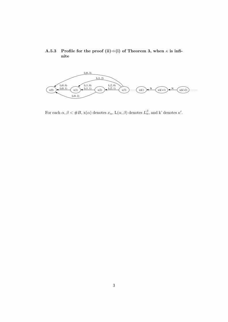
A.5.3 Profile for the proof (ii)⇒(i) of Theorem 3, when κ is infi-nite

x(0) x(1)

L(0, 0)L(0, 1) x(2)

L(0, 2)

L(1, 0)L(1, 1) x(3)

L(0, 3)

L(1, 2)

L(2, 0)L(2, 1) x(k') x(k'+1)N x(k'+2)N

For each α, β < #B, x(α) denotes xα, L(α, β) denotes Lβα, and k’ denotes κ′.

3