MPRAMunich Personal RePEc Archive

Modern Knowledge Based Economy:all-factors endogenous growth model andtotal investment allocation.

Michael Bormotov

Canadian Economics Association

10. January 2010

Online at http://mpra.ub.uni-muenchen.de/19932/MPRA Paper No. 19932, posted 18. January 2010 07:55 UTC

1

Modern Knowledge Based Economy:

all-factors endogenous growth model

and total investment allocation.

The working paper (first draft).

By Michael Bormotov

Abstract

The core problem in focus of this paper is studying how modern economy can keep

sustained growth in terms of increasing reliance on both knowledge and human capitals and

dependence on continuously depleting non-renewable natural resources.

The aim of this paper is to bridge in some way the gap between macroeconomic growth

models and models of technological evolution.

The ultimate goal of this work is to determine the optimal rate of savings and the optimal,

i.e. delivering maximum cumulative consumption during given period , total investment

allocation among physical capital, human capital, natural capital and knowledge capital, all

subject of endogenous growth, for the modern knowledge based economy where savings are

the unique source of investments.

Extended to four factors the neo-classical CES production function including physical

capital K, human capital L, raw materials (natural capital) R and knowledge capital A in three

different forms: for perfect substitution, for the case of no substitution and for the case of

unit elasticity of substitution, is accepted as the basic growth model.

There are four most important features which distinguish our all-factors endogenous

growth model from basic endogenous growth model:

- The total national capital stock which reflects the growth potential of economy is considered

consisting of four parts: physical capital, human capital, natural capital and knowledge capital.

Therefore our model embeds all four factors of production (physical capital, human capital,

natural capital and knowledge capital) as opposed to three factors (physical capital, labour and

knowledge) included in Romer model.

- The labour, represented by Human capital, is not assumed equal to population and is

measured in money units (total earnings of qualified labour which is considered equal to total

2

household income). Investments in Education system transform Population in Human capital.

Therefore in our model labour supply grows proportionally investments in human capital,

whine the path of population growth is given exogenously according to exponential or

logistics curves.

- Marginal rate of consumption and consequently marginal rate of savings are assumed

constant during exploring period; they are not given as initial conditions but are subject of

optimisation inside the model.

- Growth of every of four employed factors is considered depending on investments in

corresponding sector of economy only. It is assumed that investments, measured in money

units, absorb and exhaustively represent all underlying resources (physical capital, labour, raw

materials).

A three steps algorithm for finding the optimum solution is created. The first step defines

in general an optimum structure of investment allocation among K, L and R. The second step

defines optimum investment allocation between A from one hand and all other factors from

the other hand. The third step applies defined optimum value on optimum structure.

Key words: knowledge based economy; economic cycles; endogenous growth; investment;

optimisation; knowledge capital; human capital; natural resources.

3

Contents

1. The background ……………………………………….. 4

2. Endogenous and Exogenous factors of growth………... 11

3. Diminishing returns versus increasing returns………... 14

4. The character of return on investments in knowledge... 16

5. Selecting the type of model…………………………….. 18

6. The rate of savings and sustained growth……………… 20

7. Substitution of Natural capital by Knowledge capital…. 24

8. The concept of all-factors endogenous growth ………… 26

9. Embedding Knowledge into growth model…………….. 29

10. Investments in Knowledge Capital…………………….. 33

11. Knowledge capital flow and economic cycles…………. 36

12. A problem of dimensions……………………………….. 41

13. Natural resources in growth model……………………. 44

14 . The Human Capital……………………………………. 47

15. Lags between investments and growth………………… 49

16. The all-factors endogenous growth model…………….. 51

The Case of Perfect Substitution……………………….. 51

The Case of no Substitution……………………………... 54

The Case of Unit Elasticity of Substitution…………….. 56

17. Application of the model………………………………… 58

Conclusions……………………………………………….. 65

References………………………………………………… 71

4

1. The background

The internal mechanism of long run business cycles cannot be satisfactorily drawn from

market supply-demand fluctuation caused by entrepreneur extreme self-confidence leading to

overproduction or by customer misleading expectations, because the market itself is able to

compensate such kind of turbulence in relatively short periods, which normally do not exceed

5 years, i.e. the duration of the Kitchin cycle (3–5 years). (Bormotov, 2009).

Proceedings devoted to technological and techno-economic paradigm (e.g. Dosi, 2008;

Perez, 2004) give general explanations on how qualitative events of technological evolution

cause quantitative macroeconomic fluctuations. The details of the mechanism and its links to

macroeconomic growth models are still left blurry.

The core problem in focus of this paper is studying how modern economy can keep

sustained growth in terms of increasing reliance on both knowledge and human capitals and

dependence on continuously depleting non-renewable natural resources.

The aim of this paper is to bridge in some way the gap between macroeconomic growth

models and models of technological evolution.

The ultimate goal of this work is to determine the optimal the optimal rate of savings s and

the optimal investment allocation for economy where savings are considered as unique source

of investment capital IΣ , I

Σ = (1 – s)Y, which is exclusively responsible for endogenous

growth of all production factors (i.e. physical capital K, human capital L, raw materials

(natural capital) R and knowledge capital A) provided that the structure of total investment

allocation IΣ=I

K +I

L+ I

R+ I

A is optimal, i.e. delivers maximum to the target function which is

considered total cumulative consumption during period [0,T].

Investments in capital formation are restricted to total savings effectuated by both,

households and businesses in previous periods (i.e. fresh and vintage savings). Total

investments may not exceed the amounts of total savings. The value of total investments may

be less than total savings by the portion which gets immobilized on saving accounts, in

government bonds, etc. Any money injections, which are not accompanied by proportional

growth in goods and services supply, drive an economy away from the equilibrium. There is a

lag between increasing of Government spending and the reaction of the economy in form of

increasing supply. During this period an economy has to works in stressed regime,

5

characterised by inflation and ―chip‖ money supply. The final balance of positive and negative

consequences of this kind of regulations appears to be unpredictable for every particular case.

If Government through Central Bank ―create‖ extra investment capital by turning on the

printing machine and issuing unsecured money it leads to rising of inflation, blows up

investment bubbles and consequently drive economy to unavoidable slow down.

S D

Figure 1. Demand-Supply circle

Figure 1 illustrates how supply S creates demand D and in turn how demand D creates

supply S in the circle model. Increasing in production leads to increase in household and

business income i.e. extends total purchasing capability, i.e. increases demand. In short run the

increasing in demand is not necessarily proportional to the increasing in supply. Total

purchasing capability (TPC) is a total solvable demand corrected to present value. The TPC of

an amount of current month’ money C, t months in future, can be calculated as following:

where i denotes assumed future monthly rate of inflation.

There are some natural limits for swings in aggregate demand and aggregate supply (Figure

2). Growth of aggregate supply is limited by quantity and quality of available production

factors. Aggregate demand has to fluctuate inside the corridor, composed by the aggregate

purchasing capability or total amount of money available for purchasing, from one side, and

by the value of aggregate minimum consumer basket, along with minimum Government and

business spending that let the economy to run normally, from the other side.

6

P D

Peq

S

Smin D/Seq Dmax Smax Y

Figure 2. Demand-Supply corridor.

The value of total purchasing capability is assumed consisting of following parts that are

categorised analogically to total income (gross value added product based measure):

- Compensation of employees (wages and salaries);

- Operating surplus (gross profit, rent and interest of firms, government and other institutions);

- Mixed incomes;

- Taxes minus Subsides on products;

- Tax minus subsidies on production (other than those on products).

Figure 3 depicts the circular flow of income.

Business Injections

Consumption of Abroad

Factor domestic goods payments and services

Banks Government

Net savings Net Taxes Export expenditures

Household Withdrawals

Figure 3. The circular flow of income

Source: “Aggregate Demand and Supply and Macroeconomic Problems‖

www.bized.co.uk/educators/he/pearson/workshops/adas.htm

7

Despite assuming sustained economic growth and using constant basic prices

comparability sake we however do not apply to our model the classical term of a steady-state

growth as specified by Léon Walras (1874) and Gustav Cassel (1918). We do not consider a

uniform rate of growth when primary factor supplies, consumer demands and the outputs at

every period are growing at a constant rate and proportions of employed factors and produced

goods cannot be changed. Contra versa, in our model proportions between factors and goods

produced are subject of change due to new knowledge implementation and rate of growth is

not an initial prerequisite but a function derived from total output, rate of savings and

investments allocation among four production factors at every step of economic growth.

Similarly to Smulders (2004) we assume that the resource inputs flow must decline over

time and cumulative resource input over the given horizon is bounded, while cumulative

production is considered unbounded.

Output is produced by employing factors of production. There are four inputs or production

factors in our model: ―Physical capital‖, ―Human capital‖ (see Becker, 1964), ―Knowledge

capital‖ and ―Raw materials‖. All production factors are considered endogenous. Growth of

Physical capital depends exclusively on related investments and is assumed technically

unbounded. Growth in Human capital depends on investments in education and professional

training and is limited by population that is subject of exogenous alterations. Knowledge

capital is considered theoretically unlimited and depends on investments involved. Growth in

Raw materials supply depends on investment in exploring and extraction of natural resources

and is restricted to available (discovered) natural deposits. The availability of natural resource

evolves over time.

In macroeconomic growth theory the total output reflects the wealth of economy

adequately if it is cleaned thoroughly from any traces of inflation; otherwise the results may

be misleading. Natural resource becomes more and more expensive over time because of

scarcity. Thus naturally caused growth of prices on natural resource, especially energy (oil,

natural gas, coal), affects all basic costs and in turn lifts prices on all other goods and services,

i.e. creates inflation necessarily. That hidden creeping inflation may positively transform the

figures of total output, while the real common wealth and purchase capability exhibit an

opposite tendency; therefore the careful correction on inflation is required.

8

Physical Capital embodies the man-made resources, which include the buildings,

machinery, equipment, and inventories created by all three factors (capital, land and labour).

In this sense, capital goods may be contrasted with consumer goods. The creation of capital

goods means that consumption is forgone, resulting in savings. The flow of saving becomes a

flow of investments. Expenditures on education and training are referred to as investment in

human capital. (Britannica, 2009).

It is corny fact of common knowledge which anyone can read about in any related

textbook that capital, land and labour along with magical entrepreneurship (last one is

debateable) are the factors of production and economic growth. Here are the arguments

against treating entrepreneurship as a production factor given by Schumpeter: ―This social

function [entrepreneurship] is already losing importance and is bound to lose it at an

accelerating rate in the future even if the economic process itself of which entrepreneurship

was the prime mover went on unabated. For, on the one hand, it is much easier now than it has

been in the past to do things that lie outside the familiar routine – innovation itself is being

reduced to routine. Technological progress is increasingly becoming the business of teams of

trained specialists who turn out what is required and make it work in predictable ways. The

romance of earlier commercial adventure is rapidly wearing away, because so many things

can be strictly calculated that had of old to be visualized in a flash of genius.‖ (Schumpeter,

1942: 132; cited from Langlois, 1991). The epic ―entrepreneurship‖ is inherently

technological and business knowledge rather than a matter of individual talents or mystic art

like a Smith`s ―invisible hand‖ and now deserves be replaced by the category of ―knowledge‖.

Therefore it appears obvious that economic growth depends on existence, quantity and

quality of capital, land labour and knowledge. If so, economic growth models should include

all those factors, and do not be restricted to capital and labour only as neoclassical models do.

Economists while studding economic growth should not neglect any of growth factors.

Example of United Arab Emirates shows how possessing of natural resources may turn

rapidly a feudal society into modern civilization. Example of Japan demonstrates a jump into

post-industrial community with no natural resources, just by increasing stock of knowledge

and growing national human capital. Any factor matters while exploring the mechanism of

economic growth.

9

It is obvious that economics is all about managing of scarce resources. Therefore it seems

merely illogic to skip natural resources in growth models. It could be reasonable a while ago

for studding purposes and simplicity sake when the scarcity was not so strict like now. Labour

and natural resources then were assuming unlimited and thereby were often put apart of

considerations. Knowledge was out of the scope of mainstream economics because of

miserable share of knowledge based goods and services in total output. Now times have been

changed. Convenience of calculation cannot be a priority while exploring how modern

economy works and explaining what the mechanism of its growth is. In terms of knowledge

based economy we have to differentiate population and qualified labour. Population may be

transformed into qualified labour through proper education and training, i.e. by creating

human capital. Thereby modern economic requires four kinds of investments for growth:

investments in physical capital, investments in human capital, investments in natural resources

and investments in knowledge capital.

Summarising, let us assume that the economic growth model can be formulated as

following

Y=f(K,L,R,A)

Where: Y – total output;

K – physical capital;

L – human capital;

M – natural resources (natural capital);

A – knowledge capital.

Total output does not represent the current welfare of population adequately since

includes capital formation. There is a perennial problem of preference: spending versus

saving, current welfare versus future welfare. On our opinion total consumption CΣ 0,T during

certain period of time [0,T] reflects household welfare more realistically:

CΣ 0,T = 𝑐𝑡

𝑇0 Yt

where ct denotes marginal rate of consumption.

Yearly consumption is assumed as a constant percentage of total yearly output.

10

A cumulative consumption per capita during given period of time is recognised in this paper

as a sufficient welfare criterion also.

11

2. Endogenous and Exogenous factors of growth.

In order to distinguish between endogenous and exogenous factors of economic growth first

of all we have to determine where the border of economy is situated. If the border is demarked

properly, then all factor, that fall inside the border should be considered endogenous, and all

other factors, that affect the economy from outside the border appear to be exogenous.

Let us start with several common definitions of economy.

―The term ―economy‖ refers to the institutional structures, rules and arrangements by

which people and society choose to employ scarce productive resources that have alternative

uses, in order to produce various commodities over time and to distribute them for

consumption, now and in the future, among various people and groups in society. In a free

market economy such as Canada’s, the laws of supply and demand determine what, how and

where goods and services will be produced, and who will consume them and when. A

―strong‖ or ―healthy‖ economy is usually one that is growing at a good pace.‖

(http://www.canadianeconomy.gc.ca/English/economy/economy.html)

―The system of production, distribution and consumption; the efficient use of resources;

frugality in the expenditure of money or resources.‖ (wordnetweb.princeton.edu/perl/webwn)

―(1)Careful, thrifty management of resources, such as money, materials, or labour. (2)The

system or range of economic activity in a country, region, or community. (3) An orderly,

functional arrangement of parts; an organized system.‖

(http://www.thefreedictionary.com/economy)

―(1) The management of the income, expenditures, etc. of a household, business,

community, or government. (2) Careful management of wealth, resources, etc.; (3) restrained

or efficient use of materials, technique, etc.; (3) a system of producing, distributing, and

consuming wealth.‖ (http://www.yourdictionary.com/economy)

―Entire network of produces, distributors, and consumers of goods and services in a local,

regional, or national community.‖

(http://www.businessdictionary.com/definition/economy.html)

―(1) Activities related to the production and distribution of goods and services in a

particular geographic region. (2) The correct and effective use of available resources.‖

12

(http://www.investorwords.com/1652/economy.html)

The summarised definition based on given above may be formulated as following:

―The term ―economy‖ refers to entire network of produces, distributors, and consumers of

goods and services taken worldwide, in particular country, region, or community; to activities

related to production, distribution and consuming of goods and services undertaken by a

household, business, or government; and to careful, thrifty, restrained and efficient

management and arrangements by which they choose to employ scarce productive resources

that have alternative uses‖.

Even elementary analysis of this compiled definition shows that at least ―activities related

to the production‖ and ―arrangements by which they choose to employ scarce productive

resources‖ should necessarily include researches, developments and consequent innovations

that result in technology improvements. Ergo, applied knowledge, innovations and technology

are the parts of economic system and endogenous factors of growth.

Roughly speaking, all factors of production which are creating inside particular economic

system and with the means of the economic system (i.e. investments of different nature) are

considered endogenous. Although some factor of growth occupy mixed position being

partially endogenous and partially exogenous.

Let us roughly classify which particular factors of growth stay inside, outside and on the

border. Nature (earthquakes, hurricanes etc.) and politics are definitely impact the economy

from outside. Natural resources occupy position partially outside and partially inside the

border. We have to distinguish non-recoverable natural resources (oil, coal, gas) versus

recoverable (wood/timber) and recyclable (metals) natural resources. Non-recoverable natural

resources deposits may be either potential (not available for extraction) or explored (available

for extraction). Existence, availability and value of unexplored deposits of non-recoverable

natural resources (oilfields, gas fields, coalfields, mineral deposits etc.) are exogenous factors.

Activities related to extraction, transportation and purification of natural resources as well as

related ecological activities are endogenous factors.

Human capital is positively endogenous factor since it is being created inside economy by

transforming the population in qualified labour through costly education and professional

training.

Export is partially endogenous and partially exogenous factor of growth. Quality and

13

prising of export products are endogenous. Import policy and solvency of foreign countries

are exogenous factors.

The combination of scarcity of natural resources and permanent growth of population

stimulate creation of new knowledge since new technology is the only mean that is capable to

overcome the resources scarcity.

Example: Occurring impact of oil and natural gas scarcity on world economy have

stimulated creation of bio-diesel fuel and air turbine power plants. The wide transition to

alternate sources of energy will change the structure of entire economy and severe economic

fluctuations are expected.

The range of market commodities has been recently extended dramatically by marketable

pieces of knowledge in form of untouchable information goods and services. The market is far

not restricted to preferably touchable goods any more. Hence all activities related to creation,

distribution and implementation of technological (business, commercial) knowledge should be

referred to economic activities. Therefore theoretical discussions about endogenous or

exogenous nature of techno-shifts have no subject since this is just new commodities interred

the market and created by the economic system on demand of the market. Earlier, when

technological knowledge was rather part of pure science or even art, than market

commodities, it was reasonable to consider techno-shifts as external, coming from outside,

shocks.

But external chocks still exist. They are natural cataclysms such as earthquakes, hurricanes,

surges of Sun activity, exhausting of key natural resources, severe political decisions, etc.

Some wars and distractive political decisions have visible economic background and should

be explored and classified in order to qualify if they are rather endogenous or exogenous. For

instance, painful political demarches and following war for oil fields undertaken by country

that is suffering of oil scarcity appears to be endogenous economic phenomena, rather than

mere exogenous shock. Voluntary political decisions, that affect an economy, may be

considered as exogenous shocks also. Some environment restrictions fall in the same category.

14

3. Diminishing returns versus increasing returns.

When one speaks about returns, it is tacitly supposed, that definite amount is invested in

order to gain an income (return on investments).

There is always some framework inside which the economy is running. Rural and

industrial examples are most often quoted: given plot of land, seeds and a crop; or given plant,

with constant labour and variable physical capital or constant stock of physical capital and

variable labour supply.

If we apply an analogical approach when considering human capital acquisition in form of

education and training or knowledge capital acquisition in form of R&D, i.e. recognise

particular framework, we have to arrive to similar conclusions. If the territory and the

population are given, then growing investment in education from some point will definitely

start delivering diminishing return just because of becoming surplus and unnecessarily.

Unlimited investments in R&D in particular field, or sector, or concept or project, that became

obsolesce and therefore do not bring further substantial scientific results, will necessarily

become from some point a subject of diminishing returns also.

From the other side, if we remove framework from mentioned above classical examples and

start speaking about investment in machinery in very general, then diminishing effect may

abate or disappear at all.

Diminishing return stimulate technological progress since makes business to look for

innovations in order to keep higher returns on investment capital.

Scarcity in any factor creates diminishing return of investments in all other factors and in

itself also (scare factors becomes more expensive). For instance, the scarcity of oil create

diminishing return of investments in machinery, human capital and even in knowledge until

R&D provide the economy with the solution for oil scarcity problem. Oil is far not just energy

sours, but rather a key raw material for chemical industry.

As far as all factors grow proportionally, i.e. when there are more machinery, more stuff,

more raw materials and more knowledge then no diminishing return applies. Therefore

diminishing return is a function of scarcity and of improper, asymmetric investments in

factors growth.

15

Natural resources represent naturally scarce factor (self defined) with some qualifications.

There are non-renewable natural resources (oil, coal, gas) versus renewable (wood/timber) and

recyclable (metals) natural resources. Non-recoverable natural resources deposits are scarce

indeed.

Population (―raw material‖ that is partially being transformed through education and

training in qualified labour or human capital) is a naturally scarce factor also. It is restricted to

the size of the land and environment self- recovery norms.

Physical capital is not considered a naturally scarce factor.

Knowledge is considered potentially unlimited and hence absolutely non-scarce factor.

In case when available stock of a naturally scarce factor is sufficient to meet all current

needs and there is no danger to get it exhausted suddenly then it seems possible to take that

originally scarce factor as conditionally or temporally non-scarce one. If so, naturally scarce

factor can temporally and conditionally be treated as a non-scarce one, i.e. no diminishing

return applies.

16

4. The character of return on investments in knowledge.

Increasing return and diminishing return on investments in knowledge both are existing

phenomena. Let us differentiate the total bank of knowledge and particular piece of

knowledge that is being created and added to total bank. The total knowledge has now limits.

The ken is being permanently extended by new discoveries and inventions. The process of

exploring of infinite nature is infinite itself. The more we know the more we do not know; this

is obvious. (Figure 4.) Blowing up bubble of knowledge increases the squire of its contact with

unknown permanently.

NATURE NATURA

Knowledge

Figure 4. Unlimited knowledge

Since total knowledge is unlimited, total investments in knowledge are not subject of

diminishing return. This is clear, but not absolutely clear. Let us explore the example. Total

investments available in particular period of time are restricted to savings. Let us assume that

available investment capital is being shared among investment in stock capital, in human

capital (high skilled labour), in natural resources (including environment recovery) and in

knowledge. If only investments in knowledge are not subject of diminishing return and contra

versa deliver increasing return on investments it appears reasonable to direct the lion share of

total investments into cultivation of that ―bonanza‖ to all others factor disadvantage. What

can be expected after? Most likely something similar to classical example with the given lot of

land and increasing quantity of seeds will happened. Adding more and more pieces of pure

knowledge to the stock knowledge does not mean its automatic implementation in real

economy. Practical extracting of advantages that contains in created knowledge requires new

equipment and machinery may be different raw materials, etc. If proper developing of such an

17

infrastructure is late, insufficient or ignored the advantages of new knowledge left just

potential and further unilateral investments will be bringing less and less returns analogically

to exciding investments in sowing seeds on limited plot of land do. We can track the same

regularity when exploring investments in human capital i.e. in education and professional

training. Any economy needs as much high qualified labour as it can employ and now more.

Further investments in human capital above that limit will be bringing less and less returns,

i.e. are subject of diminishing return.

Therefore investment in creation and implementation of particular piece of knowledge

(technological concept, technology, machinery, etc.) are considered subject of diminishing

return due to obsolesce, competition and limited market capacity. In some sense diminishing

return serves the economy as a stimulator of technological progress.

18

5. Selecting the type of model.

Since introduction in 1961 (Arrow, 1961) constant elasticity of substitution (CES)

functions have become extremely popular in computable general equilibrium (CGE) models

and in other applied researches, providing a whole range of possibilities with high degree of

flexibility in substitution options from no substitution (the Leontief case of fixed coefficients)

through convex Cobb-Douglas isoquants to perfect substitution (linearity) models. (Sancho,

2009).

Let us extend the neo-classical two factor CES production function to four factor model

including physical capital K, human capital L, raw materials (natural capital) R and knowledge

capital A:

(1) Y = 𝛿

𝐴0 A (αK

λ+ βL

λ +γR

λ)

1/ λ.

where α, β, γ are the share parameters, α+β+γ =1; –∞ ≤ λ ≤ 1 determines the degree of

substitutability of the inputs; and = 𝛿

𝐴0 A catch the effect of implementation of new

knowledge,

parameter δ ≥ 0 characterises the rate of knowledge influence on growth, A0 stands for basic

value of knowledge capital, A represents current level of knowledge capital, A ≥ A0.

Elasticity of substitution e = 1

1−λ . In the limit as e approaches 1, (???) transforms in Cobb-

Douglas function; as e approaches infinity there is a linear (perfect substitutes) function; and

for Leontief (perfect complements) model e approaching 0.

In the case of perfect substitution (λ = 1) the function is:

(2) Y = (αK+ βL +γR) 𝛿

𝐴

𝐴0

In the case of no substitution (λ = –∞) the function can be specified as following:

(3) Y = min{ 𝛿𝐴

𝐴0 αK

max; 𝛿

𝐴

𝐴0 A βL

max ; 𝛿

𝐴

𝐴0 A γR

max }.

In the case of unit elasticity of substitution (λ = 0) the function is:

(4) Y = 𝑏 Kα L

β R

γ(𝐴

𝐴0)δ

.

19

Figure 1 plots the Y = const isoquants for these three cases.

L

λ = –∞

λ = 1 λ = 0

K

Figure 1 CES production functions isoquants

20

6. The rate of savings and sustained growth.

Let us specify a growth function by extending an approach employed in Solow-Swan

model (Solow, 1956) :

Y=f (K, L, R, A)

where Y denotes total output and K, L, R, A stand for physical capital, human capital, natural

capital and knowledge capital respectively.

The function is assumed to vary continuously with all factors.

Physical capital is considered a subject of depreciation with constant rate d; human capital

and knowledge capitals are assumed subject of obsolesce with constant rate ω; natural capital

is being depleted with the rate e.

Aggregate demand is assumed equal to aggregate supply and consequently total

investment I are equals to total savings S. Total savings is considered a function of total

output Y and marginal propensity to consume c

S = (1-c)Y or S = sY

where s = (1-c) denotes the marginal propensity to save.

Therefore I = sY.

Total investments I are assumed to be split in four portions, one for each of factors

I = IK + I

L + I

R + I

A

where IK

, IL

, IR

and IA stand for investment in physical capital, human capital, natural capital

and knowledge capital respectively.

Investment in particular factor is assumed the only source of its growth. In case of constant

growth

K = K0 + k IK

L = L0 + l IL

21

R = R0 + r IR

A = A0 + a IA

where K0, L0, R0, A0 stand for initial values of physical capital, human capital, natural capital

and knowledge capital respectively;

k, l, r, a denote coefficients of growth.

Figure 5 illustrates the aria of conditional growth of total output in function of depreciating

physical capital, all other factor are being the same. Over the point where the curve dK crosses

the curve sY depreciation of physical capital cannot be compensated by its growth and the

total output starts decreasing, pooling in turn decreasing of total investments, that accelerates

recession.

Y d K

Y=f [K, (L0, R0, A0)]

s2Y

Yeq

s2 > s1

s1Y

K0 Kmin (1) Kmin (2) K

Figure 5.The aria of conditional growth of total output in function of depreciating physical

capital.

Let us note, that [Yeq; Kmin] represent a solution of equation

s f [K, (L0, R0, A0)] = dK

and K = K0 + k IK

consequently Kmin = K0 + k IK

min

22

and [Yeq; Kmin] is equivalent to {s f [(K0 + k IK

min), (L0, R0, A0)]; (K0 + k IK

min )}.

For keeping on sustained growth it is necessary to increase investments in physical capital

from IK

min(1) to IK

min(1).

The obsolesce of knowledge capital can be plotted analogically (Figure 6).

Y ω A

Y=f [A, (K0, R0, A0)]

s2Y

Yeq

s2 > s1

s1Y

A0 Amin (1) Amin (2) A

Figure 6.The aria of conditional growth of total output in function of knowledge capital

subject of obsolesce (all other factors being the same).

On the Figure 6 the point [Yeq; Amin] is equivalent to

{s f [(A0 + a IA

min), (K0, L0, R0,)]; (L0 + l IA

min )}.

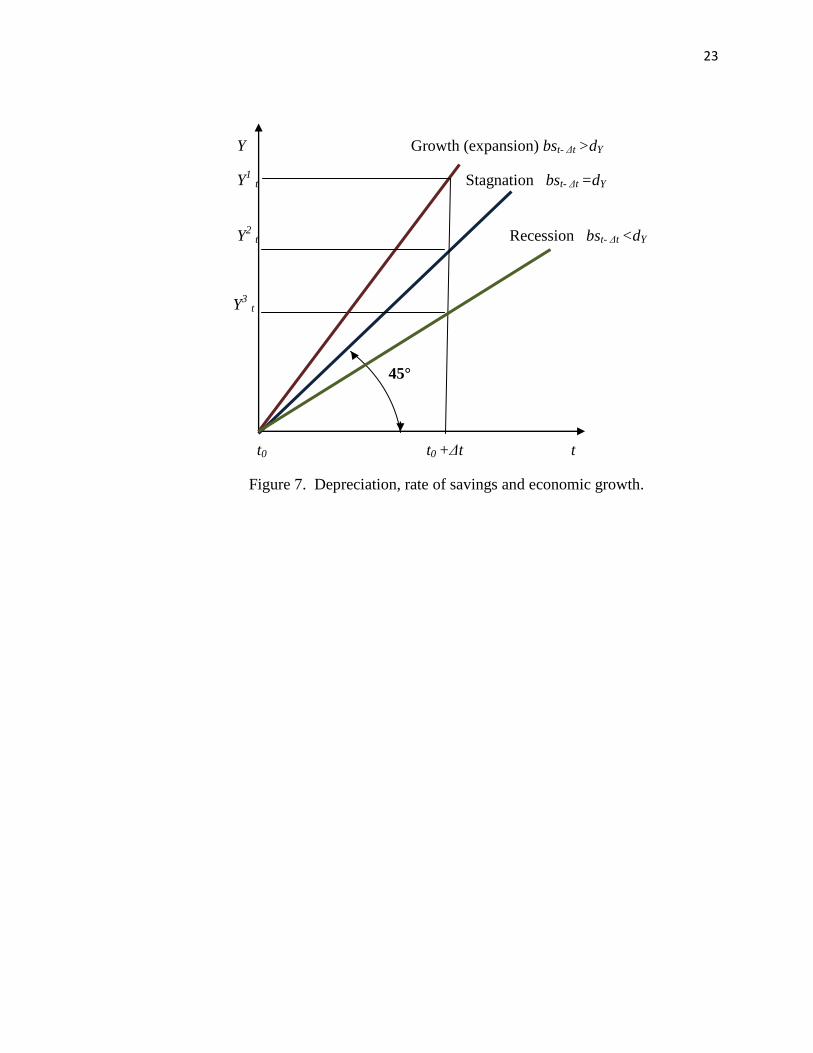
Figure 7 depicts links between rate of depreciation, rate of savings and economic

fluctuation. Depreciation of Human capital and Knowledge capital occurs due to obsolesce.

Depreciation of Natural capital is caused by depletion of natural deposits. Depreciation of

physical capital occurs due to tear and wear and obsolesce also.

23

Y Growth (expansion) bst- Δt >dY

Y1 t Stagnation bst- Δt =dY

Y2 t Recession bst- Δt <dY

Y3 t

45°

t0 t0 +Δt t

Figure 7. Depreciation, rate of savings and economic growth.

24

7. Substitution of Natural capital by Knowledge capital.

Knowledge capital substitutes partially natural resources in growth model. (Figure 8)

Y

Share of Natural

Resources in

total output Share of Knowledge

Capital in total output

t

Figure 8. Substitution of depleting natural resources by growing stock of

knowledge.

Let us assume that

RγA

δ = B = Const

Where B is a constant and (RγA

δ) is a fragment of growth function

Y = aKαL

β R

γA

δ

Let us assume that growth oh knowledge capital affect consumption of natural resources only;

all other staying the same. Then,

A(R) = (B ∕ Rγ)1∕δ

= B 1∕δ

R –γ ∕ δ

𝑑

𝑑𝑅 A(R)=( – γ ∕ δ) B

1∕δR

–(γ ∕ δ + 1)

Figure 9 illustrates the substitution of natural resources R by knowledge capital A. Curves Y1

and Y2 are represented by so named indifference curve i.e. curves at each point of which the

substitution of one factor or combination of factors by another factor or combination of factors

keeps total output constant. The slope of an indifference curve represents the marginal rate of

substitution that is not constant.

25

Rγ

KL

Y = Y2

Y = Y1

Aδ

Figure 9.

Figure 10 illustrates the substitution of natural resources R by combination of two factors

(physical capital K and human capital L)

,

Rγ

ΔA

Y = Y2 , A = A2

Y = Y1, A = A1

KαL

β

Figure 10.

On the figure the up shift of the curve from Y1 to Y2 occurs due to growth of knowledge capital

A from level A1 to level A2.

26

8. The concept of all-factors endogenous growth.

Our concept describes how the amalgamation of physical capital K, human capital L,

natural capital R and knowledge capital A, embedded in roundly endogenous growth model

produces consistent over time output delivering maximum welfare to population.

There are four most important features which distinguish our all-factors endogenous

growth model from basic endogenous growth model.

1. The total national capital stock which reflects the growth potential of economy is

considered consisting of four parts: physical capital, human capital, natural capital and

knowledge capital. Therefore our model embeds all four factors of production (physical

capital, human capital, natural capital and knowledge capital) as opposed to three factors

(physical capital, labour and knowledge) included in Romer model.

2. The labour, represented by Human capital, is not assumed equal to population and is

measured in money units (total earnings of qualified labour which is considered equal to total

household income). Investments in Education system transform Population in Human capital.

Therefore in our model labour supply grows proportionally investments in human capital,

whine the path of population growth is given exogenously according to exponential or

logistics curves.

3. Marginal rate of consumption and consequently marginal rate of savings are assumed

constant during exploring period; they are not given as initial conditions but are subject of

optimisation inside the model.

4. Growth of every of four employed factors is considered depending on investments in

corresponding sector of economy only. It is assumed that investments, measured in money

units, absorb and exhaustively represent all underlying resources (physical capital, labour, raw

materials).

In our model the simple economy produces output Y, by combining resources input R,

qualified labour input L, physical capital input K, and knowledge input A, all measured in

money units, and is composed of four sectors:

- exploring and extraction of Natural Resources, environment recovery and protecting;

- production of capital goods and services and final consumer goods and services;

27

- R&D or Knowledge Capital creation;

- education and training or Human Capital formation.

Natural resources sector supplies industrial sector with raw materials and energy; delivers

energy to population and in turn employs machinery, manufactured by industrial sector,

energy, that it produce itself, along with qualified labour, supplied by human capital sector

and new knowledge, produced by R&D sector. The extraction of natural resource becomes

gradually more expensive and requires increasing investments in recovery and preventive

protection of environment.

Industrial sector manufactures heterogeneous machines combining raw materials and

energy, supplied by natural resources sector with capital goods and services that it produced

itself, qualified labour provided by human capital sector and knowledge capital, produced by

R&D sector.

Education and training sector transforms population into qualified labour by employing

produced by itself high qualified labour (professors and instructors), knowledge capital (stock

of codified academic knowledge, codified applied knowledge, and tacit knowledge),

laboratory and training equipment, energy and few sample raw materials.

R&D sector employs human capital, laboratory and experimental equipment, energy and

some sample raw materials and produces new knowledge which being added to total stock of

knowledge increases knowledge capital.

Y = f (K,L,R,A)

Y = C + S

I = S

IK

+ IL + I

R + I

A = I

Y0 = f (K0,L0,R0,A0)

L ≤ P

R ≤ D

Neo-classical production functions assume diminishing return for either single factor and

constant return on scale for both factors altogether. We adhere to the extended opinion that

28

since growing stock of knowledge is able to partially subside the scarce resources and

transform the input-output ratios it appears reasonable to assume diminishing return for

physical capital, human capital and natural resources taken separately, constant return for all

three factors taken together, unlimited return to scale for knowledge capital, and increasing

return to scale for all four factors taken together. Technically it means that the sum of factor

coefficients in growth model exceeds one.

29

9. Embedding Knowledge into growth model.

In this paper we differentiate neoclassical exogenous growth models, basic endogenous

growth model, and present all-factors endogenous growth model.

There is a technical problem of embedding knowledge capital in growth model.

Neoclassical exogenous models and endogenous models employ different approaches to

knowledge specification.

According to (Solow, 19741) the exogenous production model with exhaustible natural

resources R can be specified as the following

Y(t) =emgt

LgR

hK

(1-g-h)

where emgt

stands in place of total factor productivity

ATFP and catches the effect of exogenous

knowledge growth on total output

ATFP = emgt

where mg is a rate of Hicks - neutral technical progress (Hicks, 1966) or equivalently m is a

rate of labour-augmenting technical progress.

In the ―cake-eating‖ exogenous model (Smulders, 2004):

Y(t) = eat

R(t)γ

knowledge productivity ATFP is assumed growing at a constant rate, denoted by a:

ATFP = eat

Endogenous growth models recognise two ways for improving of knowledge capital:

learning by doing and investments in R&D.

Let s assume constant return to scale for all rival factors K, L, and R, i.e. α + β + ν = 1

because of the replication argument: doubling all rival inputs should double output (Romer

1990). The stock of technological knowledge is assumed improving because of learning by

doing. Building of physical capital involves participants in the process of problems solving

and decision making therefore more experience is accumulated. Hence, the level of total factor

productivity, ATFP, is considered relaying to the stock of physical capital (Smulders, 2004):

A(t)TFP = K δ (t)

30

On our opinion ―learning-by-doing‖ improves rather human capital, then knowledge

capital, since represents a method of professional education and training.

The R&D-driven technological changes are phenomena of different nature. should be

distinguished from learning-by-doing since it is an activity separate from production.

New technologies (ideas or blueprints for new ways to produce) are modeled as a non-rival

input in production, denoted by A, that complements the rival inputs K, L, R. (Jones, 2002):

Y = KαL

β R

γ A

δ

It is assumed that innovation system produces new knowledge A on the base of existing

stock of knowledge A0 by brain efforts of researches denoted by LA exclusively, i.e. the share

of laboratory equipment and consumables in total expenses is considered negligibly small. For

instance, the invention of a new piece of software will have relied on the previous invention of

the relevant computer hardware, which itself relied on the previous invention of

semiconductor chips, and so on. (Bretschger, 2004; Groth , 2002; Jones, 1995 ; Whelan,

2007):

A = ξ Aφ

0 LλA

where parameter φ < 1 captures intertemporal knowledge spillovers, 0 < λ < 1 captures

congestion (or duplication) in research. (Smulders, 2004).

The seminal Romer’ endogenous model (Romer, 1990) describes the aggregate production

function as

Y = LY1-α

𝑥𝑖𝛼𝐴

𝑖=1

where LY is the number of workers producing output; the xi’s are different types of

capital goods, and 0 < α < 1; the marginal diminishing returns applies, not to capital as a

whole, but separately to each group of capital goods.

There are LA workers engaged in R&D creating a flow of invention that leads to production

of new capital goods; therefore A is not fixed. This is described analogically (3.12) by using a

―production function‖ for the change in the number of capital goods (Whelan, 2007):

A* = γ LAλ A

ϕ

31

The change in the number of capital goods depends on the number of researchers LA

and on the prevailing value of knowledge A.

In the simplest case when λ = ϕ = 1 growth of knowledge is directly proportional to the

number of researchers:

A* = γ LAA

Wages are assumed equated across sectors, so the R&D sector hire workers up to the

point where their value is as high as at any other sector of economy.

Summarising the above , we take in this paper all factors endogenously, recognise

―learning by doing‖ as a tacit factor of growth rather human capital then knowledge capital;

we consider the assuming that neither physical capital nor raw materials are used is R&D as

unreasonable. Therefore according to our vision the growth of knowledge capital is a function

of total investment in R&D sector of economy. The value of investments in new knowledge

creation is considered absorbing all spending on R&D, including laboratory equipment,

consumable materials, salaries and wages, etc.

Knowledge primary enhances the effectiveness of production through endogenous

technological change that stems from new technologies related R&D. Investment in

knowledge capital formation shares total investment pool with investment in physical capital

and investment in raw materials.

Physical capital consists of rival pieces of machinery and equipment, while new technologies

represent a non-rival input in production, that complements the rival inputs K, L, R. (Jones,

2002)

The production of new peaces or knowledge requires employment of professional

researches, denoted by LA and scientific laboratory equipment, denoted by KA. Since the

production of knowledge is considered substantially less material-intensive than production of

goods, the consumption of raw materials is assumed ignorable. (See: Jones 1995, Romer and

River-Batiz 1991)

A =aAbϕ LA

λ KA

κ

Where Ab denotes the basic stock of knowledge and a, ϕ, λ, κ – are coefficients.

32

The professional labour LA employed in a new knowledge creating activities is the part of total

labour supply LT and is a subject of equation

LA = LT – LP – LR

where LP and LR denotes the labour employed in production sector and in natural resources

sector respectively.

Because of lag 𝛥𝑡 which reflects the latent period of knowledge gestation growing of

knowledge cannot be considered as a continuous function of time, therefore

ΔA = 0, 𝑡 < 𝛥𝑡𝑓 𝛥𝐼 , 𝑡 ≥ 𝛥𝑡

Investments in some R&D projects may not deliver economic effect and just increases total

stock of knowledge in expected time horizon. Innovation sector accumulates knowledge and

by reaching some critical mass discharges periodically with inventions of different magnitude.

In that sense innovation system appears to be similar to a huge capacitor.

The share of investments in knowledge capital in total investments is relatively small, but

delivers non-proportion inadequately big added value. Anyway, investments in knowledge

capital should be at least sufficient for compensating knowledge obsolesce, growth of

population and depleting of natural resources.

33

10. Investments in Knowledge Capital.

There are three stages in the process of technological change. The first is invention of a

new product or process. The second is innovation, which is the transformation of an invention

into a commercial product, accomplished through continual improvement and refinement of

the new product or process. The third is diffusion, which is the process of gradually adoption

of the innovation by other firms or individuals from a small niche community to being in

widespread use. (Schumpeter,1942)

The process of technological change is initiated by a public or private investment in

research and development research and development (Rothwell, 1992).The output of the R&D

activities is a knowledge capital that is the intangible asset which is necessarily being used

along with other inputs while generating revenues. The value and allocation of investment in

the knowledge, knowledge spillovers and diffusion are at least partly governed by profit

incentives (Griliches, 1979).

The cycle of life of new superior technology is typically follows an S-shaped (logistic)

curve (Rogers, 1995).

The fraction of potential users that adapt the new technology rises only slowly in the early

stage, then gets faster, then slows down again as the technology reaches maturity and

approaches saturation. Experience with a technology leads to a gradual improvement over

time as a function of learning processes: learning in R&D stages, learning at the

manufacturing stage (―learning-by-doing‖) and learning as a result of use of the product

(―learning by using‖) (Rosenberg 1982, sited from Löschel, 2001).

Investments in Knowledge Capital are accumulated inside Innovation System and when the

stock of knowledge reaches some critical value it erupts with inventions of different

magnitude. According to the concept being employed in this paper the growing stock of

knowledge capital follows recurrent cycle of 45 - 60 years, the duration which corresponds to

Kondratiev wave. Knowledge capital periodically reaches some ―critical mass‖ and then

erupts with inventions of different magnitude. Every 45 - 60 years cycle starts on the platform

of previous major basic invention and by the end of the first 7 – 12 years, corresponding to

Juglar cycle, innovation system generates a minor basic invention. Then by the end of the next

7 – 12 years or 15 – 25 consequent years from the beginning (Kuznets cycle) it erupts with

34

medium basic invention. After that, on the ground of mentioned medium invention during

next 7 – 12 years knowledge capital produces another one minor basic invention and by the

end of the cycle (45 - 60 years in row from the beginning) finally erupts with new major basic

invention which serves as a platform of the next generation of growing cyclical movements.

(Figure 11). Innovations serve as an interface between Knowledge Capital, formatting by

Innovation System, and the market.

A Next major basic

invention

Enviloping S-curve minor basic invention

Previous major basic

invention medium basic invention

minor basic invention

10 25 35 50 t

Figure 11 The hypothetic step pattern of Knowledge Capital growth.

The value of total investments in less than total savings by the portion which gets immobilized

on saving accounts, in government bonds, etc. For some period Δt they are taken out of

income but do not deliver any economic effect.

There are some return-on-scale issues related to R&D investment: inventions appear more

often if more resources are invested in research and development activities. R&D may not

result in creating any marketable product by the end of the period planned beforehand, but

deliver it later, after more efforts have been invested. That regularity is assumed to be

describable by stochastic model employing Bernoulli distribution with probability density

function P(t) and distribution function D(t),

35

𝑃 𝑡 = 1 − 𝑝 𝑓𝑜𝑟 𝑛 = 0𝑝 𝑓𝑜𝑟 𝑛 = 1

𝐷 𝑡 = 1 − 𝑝 𝑓𝑜𝑟 𝑛 = 01 𝑓𝑜𝑟 𝑛 = 1

Parameter p is assumed dependable in function of total investments IA

i(t) in particular project

i:

p(IΣ)=1 – e

– δ f(I)

where 0 ˂ δ ≤ 1 is a coefficient catching a sensitivity of parameter p to growth of

investments and

𝑓 𝐼 = 𝐼 𝑡 𝑑𝑡𝑡

0

represents total investments in particular R&D project made from the beginning up to instant

of time t (reconsidered from Dosi, 2008, page 8).

The portion of investments in knowledge which did not deliver marketable effect inside

expected period could not be considered wasted, but contra versa is being accumulated in the

foundation of oncoming more important inventions. Technically, the more R&D efforts are

undertaken the more drastic results may be inspected. The value of scientific research depend

primary on value of investments, assuming all other resources are available for money.

Implementation of knowledge leads to changes in structure of production cost and brings

new features to final products. Knowledge reduces the share of raw materials and energy for

benefit of capital depreciation and added value (high-tech equipment and high qualified

labour). Growth of fractions of capital depreciation and wages is smoothed by the related

growth in productivity of capital and labour since more expensive equipment and labour are

normally producing more output per time unit.

36

11. Knowledge capital flow and economic cycles.

Due to ―Capacitor effect‖ of innovation system which regularly erupts with a surge of

inventions after relatively calm period of latent knowledge accumulation along with a lug

effect caused by lumpy nature of investments in physical capital, human capital and natural

resources, the general growth trend of total production function is interfered and complicated

by fluctuations of different durations, amplitude and severity.

Economic growth is not a continue function but a function with discontinuities. ―If all

factors were infinitely divisible, the production function would be continuous and we could

move about on it by infinitesimal steps. Many factors, however, are not infinitely divisible but

available only in such large minimum units—think, for example, of a railroad track or even a

steel plant—that product responds to addition of a unit not by a small variation but by a jump,

which means that the production function is discontinuous in such points. Such factors we call

lumpy.‖ (Schumpeter, 1939: 31)

“…the man who saves obviously does something either to change his economic situation or

to provide for a change in it which he foresees…‖ (Schumpeter, 1939: 32)

―…lags may result from causes other than technological. Friction is an example. The

reader may think of costs incident to change of occupation or to … shift from the production

of one kind or quality … to another, or to the exchange … of one asset for another, or of the

resistance to change of some prices or of the difficulty of adapting long-time contracts or of

persuading oneself … to act, and so on.‖ ―(Schumpeter, 1939: 43)

―In fact if the large plant needed in a branch of manufacture is fully occupied, and cannot

be rapidly increased, an increase in the price offered for its products may have no perceptible

effect in increasing the output for some considerable time‖ ( Marshall, 1920, Book V, chapter

XII).

Investments in physical capital, human capital, knowledge capital, natural resources deliver

growth after a latent periods, that are different in length (duration). There is no economic

effect in production sector related to investments in R&D such as new job creation, reduction

of cost or output growth during a latent period. Some effect of investments occurs just inside

R&D sector which is substantially smaller than production one. Growth of R&D sector is

37

unable to compensate the hardships caused by stagnation. Therefore the bottom line during the

latent period is negative.

Earning profit is the only or at least the major reason for entrepreneur for running

business. An economy exists in particular time and place. Unleashed entrepreneurship does

not know limits and cause overproduction. This is a part of nature of economic system, its

core, basic, fundamental attribute. New technology allows earning profit due to contraction of

cost, new utility obtained, or both factors altogether. Capital is always on watch for higher

interest and moves where actual profit or profit expectations are higher. ―It was not supposed

that the Production Function would remain unchanged over time; it would be shifted by the

discovery of new techniques of producing - that is to say, by invention. Inventions … would

not be adopted unless they raised the Social Product … It seemed to me that rises in wages …

would encourage the adoption of inventions which economised in Labour and so were biased

against Labour…‖(Hicks, 1973). Competition, namely the threat of losing profit, losing

business or being pushed out of market along with looking for higher profit and wider market

share, stimulates innovations (Figure 12).

Marginal (maximum) market price

P, C

Price

Profit

Cost

Marginal (minimum) production cost

t

Figure 12.

Innovations allow either to low cost or to rise price proportionally to value added.

Technological advantages let more output to be produced with the same input, or the same

output with fewer inputs (for example, ―just in time‖ logistic technology, etc.).

38

Approximately two massive investments attacks happen that correspond to two subordinate

cycles in every hyper-cycle. After that any further substantial investments inside the the same

technological concept are considered unreasonable. It means that expected total extra profit

doesn’t compensate required extra investments reliably, or expected interest earned on

investment is lower than one that non-risky capital shelters offer.

The model catches economic cycles related to technological evolutionary and

revolutionary changes in two ways.

The first, there is a latent periods for basic inventions gestation that makes investments in

R&D ―frozen‖ for years or even for decades. It hurts the economy, but not too hart because

total spending on R&D never exceed 10% of GDP and are spread over the time.

The second phenomenon appears much more influential. Flow of secondary inventions

grows slowly during the period following straightforwardly the new basic invention. After

that, when the invention got vide dissemination the surge of consequent invention arises. Then

during the period preceding next basic invention the big wave abates and finally ceases.

Inventions deliver opportunities for business innovations and growth. The higher density

of invention flow the more opportunities for economic growth are being employed and contra

versa the rarer frequency of inventions the fewer business opportunities are available.

Growth of stock of knowledge ΔA is assumed as a function of one argument -

investments in knowledge capital IA . Due to both ―capacitor effect‖ and lag effect growth of

knowledge capital may be preferably approximated by logistic function:

A(I) = 𝐵

1+𝑉exp (−𝛿𝐼𝐴 )

where B, V and δ – parameters of the S-curve,

I = IA

tΣ = 𝐼(𝑡)𝑑𝑡𝑇

0.

In the simplest case IA

tΣ= iA

tT

where iA

t stands for average yearly investment in R&D and T for the number of years.

or by combination of two exponential functions:

39

A(IA)=

𝐴0 𝑒xp 𝛿 𝐼𝐴 at accelerated growth faze

𝐴0 𝑒xp −𝛿 𝐼𝐴 at slowing down growth faze

or in a most simplified case as a linear function

A= 𝐴0 , 𝐼 < 𝐼𝑐𝑟

𝐴0 + 𝛿𝐼𝑐𝑟 , 𝐼 = 𝐼𝑐𝑟

The Figure 13 illustrates the models given above.

A

A= 𝐴0 + 𝛿𝐼𝑐𝑟

A(I) = A0 exp(−𝛿𝐼) A(I) = 𝐵

1+𝑉exp (−𝛿𝐼)

A(I) = A0 exp(𝛿𝐼)

A0

Icr IA

Figure 13.

Alterations in value of knowledge capital A affects productivity of physical capital K,

human capital L and effectiveness of use of natural resources R. Consequently all other

factors become involuntary involved in fluctuations following with some retard the knowledge

dynamics pattern with even wider swings that knowledge capital does due to effect of

amplifier, similar to how slide pressure applied on gas pedal makes heavy vehicle to run faster

or miserable movement of brake pedal slows it down. Knowledge capital serves like a

regulator for entire economy and makes it sound loudly or quieter just with light turn of

40

investments in R&D button. In other worlds, investments in knowledge capital IA affect

effectiveness of investments in all other factors responsible for economic growth, namely IK,

IL

and IR.

41

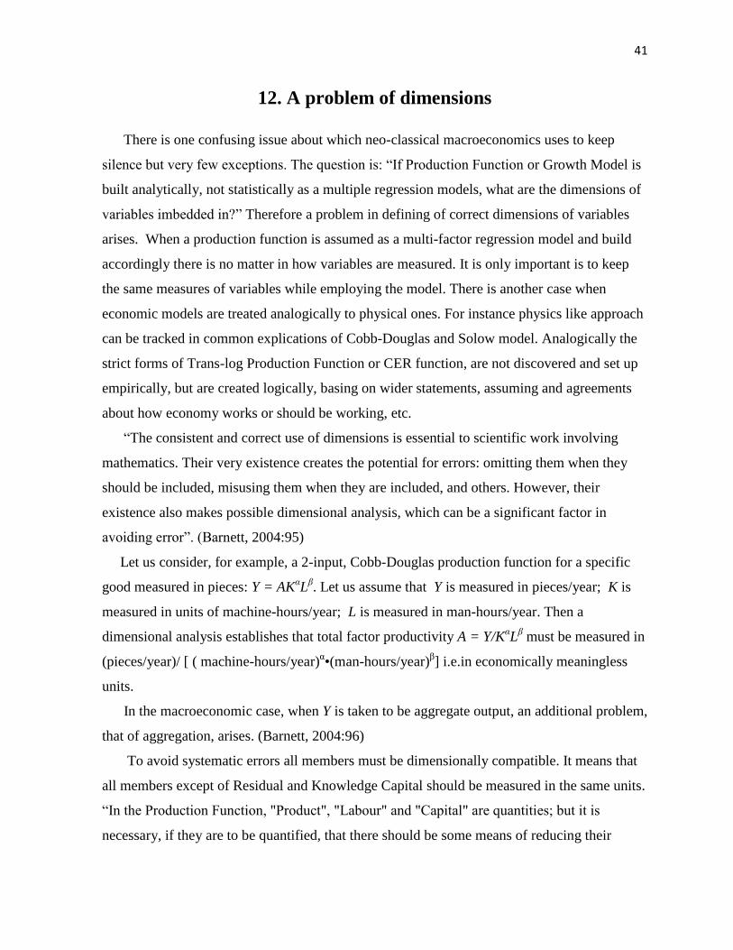
12. A problem of dimensions

There is one confusing issue about which neo-classical macroeconomics uses to keep

silence but very few exceptions. The question is: ―If Production Function or Growth Model is

built analytically, not statistically as a multiple regression models, what are the dimensions of

variables imbedded in?‖ Therefore a problem in defining of correct dimensions of variables

arises. When a production function is assumed as a multi-factor regression model and build

accordingly there is no matter in how variables are measured. It is only important is to keep

the same measures of variables while employing the model. There is another case when

economic models are treated analogically to physical ones. For instance physics like approach

can be tracked in common explications of Cobb-Douglas and Solow model. Analogically the

strict forms of Trans-log Production Function or CER function, are not discovered and set up

empirically, but are created logically, basing on wider statements, assuming and agreements

about how economy works or should be working, etc.

―The consistent and correct use of dimensions is essential to scientific work involving

mathematics. Their very existence creates the potential for errors: omitting them when they

should be included, misusing them when they are included, and others. However, their

existence also makes possible dimensional analysis, which can be a significant factor in

avoiding error‖. (Barnett, 2004:95)

Let us consider, for example, a 2-input, Cobb-Douglas production function for a specific

good measured in pieces: Y = AKαL

β. Let us assume that Y is measured in pieces/year; K is

measured in units of machine-hours/year; L is measured in man-hours/year. Then a

dimensional analysis establishes that total factor productivity A = Y/KαL

β must be measured in

(pieces/year)/ [ ( machine-hours/year)α•(man-hours/year)

β] i.e.in economically meaningless

units.

In the macroeconomic case, when Y is taken to be aggregate output, an additional problem,

that of aggregation, arises. (Barnett, 2004:96)

To avoid systematic errors all members must be dimensionally compatible. It means that

all members except of Residual and Knowledge Capital should be measured in the same units.

―In the Production Function, "Product", "Labour" and "Capital" are quantities; but it is

necessary, if they are to be quantified, that there should be some means of reducing their

42

obvious heterogeneity to some kind of uniformity. For none of the three is the reduction a

simple matter; it cannot be solved, even in the case of Labour, by counting heads or by

counting man-hours. The crucial problem, however, is that of capital. Capital, here, must

mean physical capital goods; it is an aggregate of physical goods which we have to represent

by a single quantity. As is now well known … there are just two cases in which this can be

done without error … One is the obvious case in which all components change

proportionately; the other … is that in which the price-ratios between the goods, or their

marginal rates of substitution, remain constant.‖ (Hicks, 1973)

Econometrics models are very diverse due to mostly being united in the form of

―special cases‖ and generally do not confined to any a priori given "supermodel". Economists

use to find the unique sets of variables which best describe the subject of studies. Thus the

check of dimensions for all employing variables and in order to test the correctness of the

models appears to be mandatory in economics the similar way as in physics. The

"considerations of dimension‖, in fact serve as additional conditions and may precede the

creation of a new models, and even serve as a priori requirement for these models.

The "considerations of dimension" have long been effectively used in the physics to verify

the correctness of the equations (Pospelov, 2006). Comparison or the addition of quantities

measured in different units indicates the presence of errors. On the other hand, knowledge of

dimensions of some variables can help to specify correctly the dimensions for others, even

without a detailed account of equations describing the process. That method of model analysis

has been undeservedly left out of scope of the researches building econometrics models. Let

us recall what such a system of units is by the experience of physics. The basic units in the

International System of Units (SI) are: kg, meter, second, ampere, Kelvin, luxury. Such item

as, for example, Newton = kg · meter/sek2 is derived from the basic units.

In econometrics models all input variables are measured in natural (capita, piece, kg, m,

m2, m

3, etc.) and money units. The final output variables on macroeconomic level are most

often measured in money units. Employing ―considerations of dimensions‖ for examples to

macroeconomic growth model specified as

Y = a K

α L

βR

γ A

δ (.)

43

where Y stays for total output and K, L, R, A denote physical capital, human capital, natural

capital and knowledge capital respectively.

Let us assume that total output Y is measured in money units, namely dollars $. That

initial term sets a term on dimensions of all other variables, i.e. after calculating according to

given formula the result must be measured in plain dollars. Following KAM methodology the

stock of knowledge capital A is measured here as a index and do not affect the dimension of

dependent variable Y. Residual coefficient a is dimensionless also. Physical capital K and

natural resources R are measured in money units due to their heterogeneity. Considering the

above specifications, there is no other choice for measurement of human capital left but using

money units, otherwise dimensions of different variables comes into conflict that indicates an

error. The dimension testing equitation for (.) can be specified as following

$ = $α $

β$

γ = $

α+β+ γ

That equation works when α+β+ γ = 1 only. Therefore we have got one more proof of

constant return to scale for combination of three factors: physical capital, human capital and

natural resources, and of unbounded return to scale for the knowledge capital. Another one

important conclusion is that all factors imbedded in the model must have the same dimension

and be measured in money units.

44

13. Natural resources in growth model

Exhaustible natural deposits are given exogenously and assumed all available for

exploration and extraction.

Prices on raw material are basically being built under influence of two groups of factors:

depletion of exhaustible natural resources and ecological concerns. A price on natural

resources includes costs of exploration, extraction and mandatory expenses on recovery and

protection of environment. Supply of raw material decreases due to natural causes, while

demand grows, therefore prices on scarce natural resources grow permanently. There is a

level of price Pcr above which employing of traditional raw materials becomes economically

inefficient. At that point alternate materials and energy carriers get an advantage before

natural products. Examples of such a substitution are biodiesel, wind power plants, etc.

(Figure 14)

P

Price on alternate product

Pcr

Price on natural resource

0 Extraction over time 100%

Figure 14. Substitution of natural resources by alternate products

Alternative sources of raw material and energy let to solve a scarcity problem, but

environment protection issues still exist. For instance, biodiesel plants pollute environment in

some way also. This paper adheres to extended concept taking potable water, breathable air

and ozone pad as parts of natural resources.

Let S(t) be the stock of non-renewable resources available at time t, and R(t) the rate

of extraction of this resource at time t. It implies that the stock at time t equals the

stock at time zero, minus what has been extracted cumulatively between time zero and

45

t. (Dasgupta and Heal (1979), p. 154. Sited from Smulders (2004), p. 4).

In mathematical terms:

𝑆 𝑡 = 𝑆 0 − 𝑅 𝜏 𝑑𝜏

𝑡

0

Extraction can at most run down the stock completely, i.e. S(t) ≥0 for all t. This

implies that the total amount of resources that can be extracted over time is bounded

by the initial resource stock 𝑆 0 .

In case when R(t) cannot be considered as a continuous function of time the following form of

equation is provided

𝑆 𝑡 = 𝑆 0 − 𝑟𝜏𝑡0 (6.?)

where 𝑟𝜏 represents extraction of natural resources in year τ.

The equation (6.?) can be transformed in dynamic growth form

St=St-1 – rt-1 , t = 1,2… T

where T stays for the given horizon.

The Dasgupta-Heal-Solow-Stiglitz (DHSS) model was introduced for studying the role of

an essential non-renewable resource in economic growth. The reasons for this specification

varied from plausibility of this case: ―Only the Cobb-Douglas form may be said to have

properties that are reasonable at the corner‖ (Dasgupta, Heal 1974, p.14), to theoretical

interest: ―If the elasticity of substitution between resources and other factors exceeds one, then

resources are not indispensable to production. If it is less than one, then the average product of

resources is bounded. So only the Cobb-Douglas remains‖ (Solow 19742, p. 34), to technical

simplicity: ―In a Cobb-Douglas production function, we need not distinguish between labour,

capital, and resource augmenting technical progress‖ (Stiglitz 1974, p. 131), and to orientation

on subsequent numerical studies and teaching (Dasgupta, Heal 1974, p. 26). Dasgupta and

Heal (1974, p. 26) noted that this narrow specification does not restrict the results from further

46

generalization, however, as Solow (19742, p. 34) put it, ―Any extra generality hardly seems

worth striving for.‖ (Sited from Bazhanov, 2008)

For embedding the natural resources in growth model we employ the experience of

Dasgupta-Heal-Solow-Stiglitz (DHSS) model. (See: Dasgupta, Heal, 1974; Solow, 19742;

Stiglitz ,1974). The DHSS model describes a market economy with two factors of production:

a depleting stock of non-renewable natural resource and a stock of man-made physical capital

which depreciation is compensated by technical progress. The DHSS model normally assumes

population equals to labour, zero population growth, zero extraction cost, and the Cobb-

Douglas per capita production function (Bazhanov,2008)

y(t) = kα(t)r

β(t)

α, β ∈ (0, 1), α + β =1

where the depletion of natural resources is balanced by investment in man-made capital.

sustainable level of consumption. Benchekroun and Withagen (Benchekroun, 2009) provided

a closed form solution to the DHSS problem using the exponential integral function.

In our model all recyclable raw materials (metals, etc.) are considered recycled.

47

14 . The Human Capital.

The Human capital, not entire population, is considered generating total output. The rest of

employable population is assumed either employed but delivering inconsiderable share of

income due to pour qualification or merely unemployed and receiving social welfare, provided

by government.

Human Capital Theory postulates that expenditure on training and education is costly,

and should be considered an investment since it is undertaken with a view to increasing

personal incomes. Human capital can be viewed in general terms, such as the ability to use

knowledge, or in specific terms, such as the acquisition of a particular production skills.

(Becker, 1964). That theory stems from Adam Smith’s explanation of wage differentials.

(Smith, 1776). The costly learning the job is a key factor of net advantage of different

employments. All other things being equal, personal incomes vary according to the amount of

investment in the education and training which transform population in human capital.

Sufficient investments in human capital are indispensable for economic growth. (Marshall,

1998).

Total wages and salaries earning by qualified labour is assumed to be fair measure of

human capital, reflecting its market value.

Let us assume that distribution to total output obeys the Pareto Law which in generalized

form states that 80 % of effects are most likely achieved with 20 % of the employed means,

i.e. 20% of population (high qualified labour) in our case generates 80% of total value added.

Mathematically, where something is shared among a sufficiently large set of participants,

there will always be a number k between 50 and 100 such that (100 − k)% of the participants

obtain k% of sharing matters. In the case of equal distribution k =50 (e.g. exactly 50% of the

people take 50% of the resources) and nearly 100 in the case of a tiny number of participants

taking almost all of the resources. There is nothing special about the number 80, but many

systems tends to have k somewhere around. (Pareto, 1971).

United Nations Development Program (UNDP) Report gives a proof that the ratio 20:80

works on macroeconomic level. (UNDP, 1992). Table 1 shows the distribution of global

income where richest 20% of the world's population controls over 80% of the world's income.

48

Table 1 Distribution of world GDP, 1989.

Quintile of population Income

Richest 20% 82.70%

Second 20% 11.75%

Third 20% 2.30%

Fourth 20% 1.85%

Poorest 20% 1.40% Sours: UNDP, 1992.

Income growth related to advantages of new technology implementation and skill-biased

technical changes accrues to those with the higher education and skills following Pareto Law

with joint ratio even exceeding classical 20:80. For instance, there is an assessment that the

benefits of economic growth over the last 30 years have largely been concentrated in the top

1%, rather than the top 20%. (Krugman, 2006).

Human capital does not follow Walras’ regularities: real-wage does not clear the market

and involuntary unemployment as well as labour rationing are the rules. The aggregate labour

demand is calculated as a sum of labour demand of all four sectors. The endogenous aggregate

supply is absolutely elastic but limited by the number of employable population and share of

total available investments designated for human capital.

Population is assumed given exogenously and is a subject of normal exponential or S-shape

growth.

49

15. Lags between investments and growth.

There are lags between investments in particular sector and growth of corresponding factor.

Durations of lags vary for different objects of investments. For example, building up a new

plant takes substantially more time then re-equipping of existing facility, or grounding of a

medical doctor is much more long process then truck driver training, or exploring and starting

a new mine require more time then installation of a new mining machine takes, etc.

Pavitt's Taxonomy (Pavitt, 1984) categorizes industrial firms according to sources of

technology, requirements of the users, and appropriabilityin four categories:

(1) Supplier-Dominated: includes firms from mostly traditional manufacturing such as textiles

and agriculture which rely on sources of innovation external to the firm.

(2) Scale-Intensive: characterized by mainly large firms producing basic materials and

consumer durables, e.g. automotive sector. Sources of innovation may be both internal and

external to the firm with a medium-level of appropriateness.

(3) Specialized Suppliers: smaller, more specialized firms producing technology to be sold

into other firms, e.g. specialized machinery production and high-tech instruments. There is a

high level of appropriability due to the tacit nature of the knowledge.

(4) Science-based: high-tech firms which rely on R&D from both in-house sources and

university research, including industries such as pharmaceuticals and electronics. Firms in this

sector develop new products or processes and have a high degree of appropriability from

patents, secrecy, and tacit know-how.

Due to vide heterogeneity of physical capital (buildings, machinery, equipment, means of

communication and transportation, industrial infrastructure and inventories used in

production), investments in miscellaneous pieces of physical capital develop economic effect

after substantially different waiting periods. ―Every businessman realizes that running his

plant in the customary way, going through all the motions of daily business routine, is one

thing and that setting up the plant or changing its setup is another.‖ (Schumpeter, 1939: 29).

―Many factors, however, are not infinitely divisible but available only in such large minimum

units—think, for example, of a railroad track or even a steel plant—that product responds to

addition of a unit not by a small variation but by a jump…‖(Schumpeter, 1939: 31). Building

a new plant or highway from the scratch, including all infrastructures, may take much more

50

than 5 years, while re-equipment of running plant may be fulfilled in several months.

Investments in knowledge capital demonstrate even more vide diversity of lags due to

variety of latent periods of ripening requiring for different pieces of new knowledge, from 5 –

7 years for minor basic technology improvements through 10 – 15 years for medium basic

inventions to 25 – 30 years for majeure inventions driving global technological revolutions.

51

16. The all-factors endogenous growth model.

This model is not a production function but macroeconomic model for assessing

production potential of entire economy. Total output here is rather a forecast of economic

potential than assessment of real GDP. Therefore natural resources and human capital are

taken at maximum available limit. So this is not the same characteristic as statistical one. We

assume that the marginal rates of substitution of factors of growth remain constant.

The Case of Perfect Substitution

Y =b (αK + βL + γR)δ 𝐴

𝐴0

subject to:

α + β + γ = 1

δ>0

A≥A0>0

K = K0 + k IK

0 = K0 + k iK

0 s Y0

L = L0 + l I L

0 = L0 + l iL

0 s Y0 (.)

R = R0 + r IR

0 = R0 + r iR

0 s Y0

A= A0 + g IA

0 = A0 + g iA

0 s Y0

IK

0 + I L

0 + IR

0 + IA

0 = IΣ

0 = sY0

IK

0≥ IK

min

IL

0≥ IL

min

52

IR

0≥ IR

min

IA

0≥ IA

min

𝐼0𝐾

𝐼0𝛴 +

𝐼0𝐿

𝐼0𝛴 +

𝐼0𝑅

𝐼0𝛴 +

𝐼0𝐴

𝐼0𝛴 = 1

iK

0 + iL

0 + iR

0 + iA

0 = 1

iK

0≥ iK

min

iL

0≥ iL

min

iR

0≥ iR

min

iA

0≥ iA

min

Y = {α[K0 + k iK

0 (1 – s) Y0] + β[L0 + l iL

0 (1 – s) Y0] + γ[R0 + r iR

0 (1 – s)]}δ 𝑏

𝐴0 [A0 + g i

A0 (1 – s) Y0]

Let us note that all members of the above equation except of iK

0 ;iK

0 ;iK

0 ;iK

0 are constant.

Since we are not finding the exact value of output Y but looking for set of iK

0 ;iK

0 ;iK

0 ;iK

0

which delivers the maximum Y let us assume

K0 = 0; L0 = 0; R0 = 0; A0 = 1; b=1; δ = 1

(1 – s) Y0 =S0

Y = (α k iK

0 S0 + β l iL

0 S0 + γ r iR

0 S0) g iA

0 S0→max

iA

0 = 1– iK

0 – iL

0 – iR

0

Y = (α k iK

0 + β l iL

0 + γ r iR

0) (1– iK

0 – iL

0 – iR

0) g S02→max

Let us denote

(α k iK

0 + β l iL

0 + γ r iR

0) = M1

(1– iK

0 – iL

0 – iR

0) = M2

Y = M1 M2 g S02→max

53

Since (g S02) is a constant then an optimum (maximum) Y depends on values of M1 and M2 only.

M1 = M1max

when iK

0 + iL

0 + iR

0 = 1– iA

min and the maximum iN

0 , N ∈ [K, L, R] corresponds to

max{α k; β l; γ r }. It means that two of iN

0 , N ∈ [K, L, R] are equal to iN

min, N ∈ [K, L, R] and

the third is equal to

i3-rd

0= 1– iA – i

1-stmin – i

2-ndmin .

M2→ M2max

when iK

0=iK

min ; iL

0=iL

min ; iR

0= iR

min , i.e iA

0= 1– iK

min – iL

min – iR

min .

Therefore the optimum solution containing within the marked borders can be fined by three

steps algorithm. The first step defines in general an optimum structure of investment

allocation among K, L and R. The second step defines optimum investment allocation between

A from one hand and all other factors from the other hand. The third step applies defined

optimum value on optimum structure.

Let us go through example. Let us assume that the maximum iN

0 , N ∈ [K, L, R]

corresponding to max{α k; β l; γ r } is iK

0. Then the optimum structure is {(1– iA – i

Lmin – i

Rmin);

iL

min; iR

min}

Y = (α k (1– iA – i

Lmin – i

Rmin) + β l i

Lmin+ γ r i

Rmin) i

A g S0

2→max

Y = (– α k iA – α k (i

Lmin + i

Rmin – 1) + β l i

Lmin+ γ r i

Rmin) i

A g S0

2→max

Let us denote [– α k (iL

min + iR

min – 1) + β l iL

min+ γ r iR

min] = C1

g S02 = C2

Y = (C1 – α k iA ) i

A C2 →max

Y = C1C2 iA – α k C2 (i

A)2 →max

To find maximum let us use the first derivative and the second derivative tests employing

Fermat’s theorem.

The necessary condition:

𝑑

𝑑𝑖𝐴 = C1C2 – 2 α k C2i

A = 0

i A

opt =

𝐶1

2𝛼𝑘 =

1

2𝛼𝑘 [β l i

Lmin+ γ r i

Rmin – α k (i

Lmin + i

Rmin – 1)] (*)

54

The sufficient condition:

𝑑2

𝑑𝑖𝐴2 = – 2 α k < 0 , hence (*) is a maximum.

The complete optimum solution is the following:

iK

opt =1– 1

2𝛼𝑘 [β l i

Lmin+ γ r i

Rmin – α k (i

Lmin + i

Rmin – 1)] – i

Lmin – i

Rmin

iL

opt = iL

min

iR

opt = iR

min

i A

opt =

𝐶1

2𝛼𝑘 =

1

2𝛼𝑘 [β l i

Lmin+ γ r i

Rmin – α k (i

Lmin + i

Rmin – 1)]

The Case of no Substitution

Y = min{ 𝛿𝐴

𝐴0 αK

max; 𝛿

𝐴

𝐴0 A βL

max ; 𝛿

𝐴

𝐴0 A γR

max }.

This paper proposes a system of three simplified growth models. Every simplified model

employs combination of two factors one of each is a knowledge capital and another is a

physical capital, human capital or raw materials respectively. Each simplified model allows

finding the maximum total output in function of imbedded factors. Every factor taken

separately is assumed sufficient to assess a production potential of economy.

First of all there is a neoclassical (per capita) production function

Y/L = f(K/L),

specified as

y(K,A,t) = A0eδt [k(t)]

α.

55

Then the simplest model of growth with non-renewable resources, so named ―cake-eating

model‖ where output is derived from non-renewable resource input R only and the

productivity A is specified as

A(t) = A0eδt

is assumed growing at a constant rate, denoted by δ:

(6.?) Y(R,A,t) = A0eδt

[R(t)]γ

The coefficient γ captures ―resource dependence‖. The larger γ, the more a given reduction in

resource supply hurts production (Smulders, 2004).

The third is what we name a human capital productivity model. Household income amounts

to 2/3 of total GDP. Let us analogically (6.?) assume that in term of increasing reliance of

modern knowledge based economy on human capital it is possible to derive the total output

from the human capital only

(6.??) Y(L,A,t) = A0eδt

[L(t)]β

The coefficient β captures ―human capital dependence‖. The larger β, the more economy

depends on stock of human resources.

The final assessment of total output or a production potential of the economy is proposed

to carry out by employing an amalgamation of all three mentioned above models according to

following formula

Y( t) = min{ max[Y(K,A,t); max[Y(L,A,t)]; max Y(R,A,t)}

which is equivalent to:

Y( t) = min{ Y(Kmax,Amax,t); max[Y(Lmax,Amax,t)]; max Y(Rmax,Amax,t)}.

By imbedding equations given above (???) can be specified as following

Y( t) = min{ max| LA0eδI

[k(t)] α

; max| A0eaI

[L(t)]β; max| A0e

δI [R(t)]

γ}

Where

max| LA0eδI

[k(t)] α

corresponds to LA0 exp(δ𝐼max )[kmax(t)] α

;

max| A0eδI

[L(t)]β means A0 exp(δ𝐼max )[Lmax(t)]

β ;

max| A0eδI

[R(t)]γ corresponds to A0 exp(δ𝐼max )[Rmax(t)]

γ.

56

Now let us consider a simplest case when functions y(K,A,t), Y(R,A,t) and Y(L,A,t) are

linear extensions of following ratios

Δy

Δ𝑘 = rk Δy = rk Δk ΔA ΔY = rk Δk L ΔA

𝛥𝑌

𝛥𝐿 = rL ΔY = rL ΔL ΔA

Δ𝑌

Δ𝑅 = rR ΔY = rR ΔR ΔA

Following the declared simplified approach let us specify k, L, R and A as linear functions of

particular investments

k (IK) = k0 +α I

K

L (I

L) = L0 +δ I

L

R (I

R) = R0 + λ I

R

A(I

R) =

𝐴0, 𝐼 < 𝐼𝑐𝑟𝐴0 + 𝛿𝐼𝑐𝑟 , 𝐼 = 𝐼𝑐𝑟

The Case of Unit Elasticity of Substitution

The growth function is specified as

Y = 𝑏 Kα L

β R

γ(𝐴

𝐴0)δ

Let us transform it in logarithmic form

lnY = lnb + α lnK + β lnL + γ lnR + δlnA – δlnA0 (**)

57

Let us denote: Q = lnY; B = (lnb – δlnA0) ; X = lnK; H = lnL; G = lnR and E = lnA; then (**)

can written as

Q = B + α X + β H + γ G + δE

Thus, by replacing variables the Case 3 may be reduces to the Case 1.

58

17. Application of the model

This research is aimed to map the saving-investment strategy which maximise total

consumption during certain period rather than find equilibrium. The total consumption during

T consequent years is assumed as a simplified target function instead of much more

complicated classical ―utility function‖ or ―satisfaction function‖.

Variables:

s – rate of savings;

I – current investment capital;

IS

0 – initial stock of investment capital;

IK ,I

L ,I

R ,I

A – investments allocation;

Y0, S0, K0, L0, R0, A0, P0, D0, IS

0 – initial conditions

CΣ = [1 + 𝑠 𝑡 ]𝑌(𝑇

𝑡=0 𝑡)

If function C(t) is continues then

CΣ

= 𝐶 𝑡 𝑑𝑡𝑇

0= 1 − 𝑠 𝑡 𝑌 𝑡 𝑑𝑡

𝑇

0

If rate of savings is assumed constant over time, then

CΣ

=(1 − 𝑠) 𝑌 𝑡, 𝑠 𝑑𝑡𝑇

0

𝑑𝐶

𝑑𝑠= 0

It is a tempting idea to map a trajectory of savings/spending ratio which maximise total

consumption during period T, however it brings up an ethic problem of sacrificing of some

generations for benefits of others. A specific ethic problem deserves to be explored separately

and is not in the scope of this paper. Therefore, let us assume constant over rate of savings

which reflect fair equal distribution of total income between generations.

59

Let us denote total output Y for three consequent moments of time (t-Δt), t, (t+Δt) as Yt-Δt,

Yt, Yt+Δt respectively (Figure 15).

Y St+Δt

St Yt+Δt Ct+Δt

St-Δt Yt Ct

Yt-Δt Ct-Δt

t

Figure 15

Let us assume

Yt = Yt-Δt + f(St-Δt)

then

Ct = (1 – s) Yt = (1 – s)[ Yt-Δt + f(St-Δt)].

In case of linear function

f(St-Δt) = y St-Δt

where y stands for average ratio Δ𝑌

Δ𝑆 for the period [0,T]

Ct = (1 – s) Yt = (1 – s)(Yt-Δt + ySt-Δt) = (1 – s)(Yt-Δt + ySt-Δt).

By definition St-Δt = sYt-Δt therefore

Ct = (1 – s)(Yt-Δt + ySt-Δt) = (1 – s)(Yt-Δt + y sYt-Δt ) = (1 – s)(1 + y s) Yt-Δt

Analogically

Ct +Δt = (1 – s)(Yt + ySt) = (1 – s)(Yt + y sYt) = (1 – s)(1 + y s) Yt

60

Let us remind that

Yt = Yt-Δt + f(St-Δt) = Yt-Δt + ySt-Δt

Therefore

Ct +Δt = (1 – s)(1 + y s)( Yt-Δt + ySt-Δt) = (1 – s)(1 + y s)( Yt-Δt + ysYt-Δt) = (1 – s)(1 + y s)2Yt-Δt

Finally skipping routine

Ct =(1 – s)(1 + y s)tY0

where Y0 represents initial total output.

CΣ = (1 − 𝑠)𝑇

𝑡=0 (1+ y s)t Y0 = (1 – s) Y0 (1 +𝑇

𝑡=0 y s)t

Let us note that above equation represents geometric series with common ratio (1 + y s) and

first member (1 – s) Y0 , therefore the equitation can be specified as following

CΣ=

Y0

(1−𝑠)

𝑦𝑠[(1+y s)

T –1]

To define sopt that maximise CΣ let us take partial derivative

𝑑

𝑑𝑠 C

Σ. and equate it to 0. Skipping

the routine

𝑑

𝑑𝑠 C

Σ.= { s – s (1 + ys)

T[1– y(1 – s)ln(1 + ys)] + (1–s)[(1 + ys)

T –1]} ∕ ys

2 = 0

In case when the function C (t) is continues

C (t) = (1 – s) Y0 (1 +

𝑇

0 y s)

t dt

Skipping the routine:

CΣ

[0, T] = Y0 1−𝑠

ln (1+𝑦 𝑠) (e

T ln(1+y s) – 1)

Optimising rate of savings we considered that total investments IΣ=I

K +I

L+ I

R+ I

A in every

year t ∈ [0,T] are allocated among physical capital K, human capital L, paw materials (natural

61

capital) R and knowledge capital A in the most efficient way maximising the target function

which is considered total consumption CΣ

t.

yt = y(IK

t ,IL

t, IR

t, IA

t)

Ct = (1 – s) Yt

Yt = bKtαLt

βRt

λAt

δ (5)

Kt = Kt-1 + k(I K

t-1) = K0 + k(IK

0,t)

Lt = Lt-1 + l(I L

t-1) = L0 + l(I L

0,t)

Rt = Rt-1 + r(IR

t-1) = R0 + r(IR

0,t)

At = At-1 + a(IA

t-1) = A0 + a(IA

0,t)

In case of exponential growth for first three factors and logistic growth of knowledge capital

Kt = K0 + [𝐼𝑡

𝜏=0K(τ)]

k d τ

Lt = L0 + [𝑡

𝜏=0(I

L (τ)]

l d τ

Rt = R0 + [𝑡

𝜏=0IR(τ)]

r d τ

At = A0 + 𝐵𝑡

𝜏=0

𝑑 𝜏

1+𝑉 exp [−𝛿𝐼 𝑡 ]

Where IK(τ), I

L (τ), I

R(τ), I

A(τ) stay for trajectories functions of investments in physical capital,

human capital, natural resource and knowledge capital respectively.

Let us assume the most simplified case of linear function of growth when

Kt = Kt-1 + k I K

t-1

Lt = Lt-1 + l I L

t-1 (6)

Rt = Rt-1 + r IR

t-1

At = At-1 + a IA

t-1

62

By initial terms

IΣ

t-1 =

IK

t-1 + IL

t-1 + IR

t-1+ IA

t-1

Let us divide left and right parts by IΣ

t-1 > 0 then

IΣ

t-1/ IΣ

t-1 =

IK

t-1 / IΣ

t-1+ IL

t-1/ IΣ

t-1 + IR

t-1/ IΣ

t-1+ IA

t-1/ IΣ

t-1

or

1 = iK

t-1 + iL

t-1 + iR

t-1 + iA

t-1

Where = IK

t-1 / IΣ

t-1; iL

t-1= IL

t-1/ IΣ

t-1; iR

t-1= IR

t-1/ IΣ

t-1 and iA

t-1= IA

t-1/ IΣ

t-1.

Let us remind that IΣ

t-1=sYt-1 therefore

IK

t-1=s iK

t-1Yt-1

IL

t-1= s iL

t-1Yt-1 (7)

IR

t-1= s iR

t-1Yt-1

IA

t-1= s iA

t-1Yt-1

Now combining (6) and (7)

Kt = Kt-1 + k s iK

t-1Yt-1

Lt = Lt-1 + l s iL

t-1Yt-1

Rt = Rt-1 + r s iR

t-1Yt-1

At = At-1 + a s iA

t-1Yt-1

Now growth function (5) may be specified as following

Yt = b (Kt-1 + k s iK

t-1Yt-1)α

(Lt-1 + l s iL

t-1Yt-1)β

(Rt-1 + r s iR

t-1Yt-1)λ (At-1 + a s i

At-1Yt-1)

δ (8)

iK

t-1 + iL

t-1 + iR

t-1 + iA

t-1 = 1

63

Let us note that in year t al other then iK

t-1 , iL

t-1 , iR

t-1 and iA

t-1 are known constants. Therefore

we can simplify the equation (8)

Yt = b (gK

t-1)α

( gL

t-1)β ( g

Rt-1)

λ ( g

At-1)

δ (9)

where gK

t-1 = Kt-1 + k s iK

t-1Yt-1

gL

t-1 = Lt-1 + l s iL

t-1Yt-1

gR

t-1= Rt-1 + r s iR

t-1Yt-1

gA

t-1 = At-1 + a s iA

t-1Yt-1

Total consumption in year t

Ct = (1 – s) Yt = (1 – s) b (gK

t-1)α

( gL

t-1)β

( gR

t-1)λ ( g

At-1)

δ (10)

Let us transform (10) in logarithmic form

ln(Ct) =ln(1 – s) + ln b + α ln(g

Kt-1) +

β ln(g

Lt-1) + λ ln(g

Rt-1)

+ δ ln(g

At-1) → max

Subject to terms

1

𝑘 gK

t-1+ 1

𝑙 g

Lt-1+

1

𝑟 g

Rt-1 +

1

𝑎 g

At-1= const t-1

const t-1= s Yt-1+ Kt-1 / k + Lt-1 / l + Rt-1 / r + At-1 / a

gK

t-1 ≥ iKmin

t-1 k s Yt-1 + Kt-1

gL

t-1 ≥ iLmin

t-1 l s Yt-1 + Lt-1

gR

t-1 ≥ iRmin

t-1 r s Yt-1 + Rt-1

gA

t-1 ≥ iAmin

t-1 a s Yt-1 + At-1

Dispute complicated system of equations and comparisons, the maximum can be found by

employing a mere logic and common since. Since investment capital may be directed to any

factor that are being represented by gK

t-1 ,gL

t-1 ,gR

t-1 and gA

t-1 the target function reaches its

maximum value if maximum share of capital invested in factor with the biggest weight

coefficient: max{ α, β, λ, δ} while all terms are obeyed. Such a solution agrees with an

64

investment capital allocation when all factors except one with maximum weight coefficient

get minimum investments while the winning factor consumes all the balance. For instance, if

max{ α, β, λ, δ} is δ then the optimum solution is

iKopt

t-1 =

iKmin

t-1

iLopt

t-1 = iLmin

t-1

iRopt

t-1 = iRmin

t-1

iAopt

t-1 = 1– (iKmin

t-1+ iLmin

t-1 + iRmin

t-1)

65

Conclusions

1. The internal mechanism of long run business cycles cannot be satisfactorily drawn from

market supply-demand fluctuation caused by entrepreneur extreme self-confidence leading to

overproduction or by customer misleading expectations, because the market itself is able to

compensate such kind of turbulence in relatively short periods, which normally do not exceed

5 years, i.e. the duration of the Kitchin cycle (3–5 years).

2. Investments in capital formation are restricted to total savings effectuated by both,

households and businesses in previous periods (i.e. fresh and vintage savings). Total

investments may not exceed the amounts of total savings, but he value of total investments

may be less than total savings by the portion which gets immobilized on saving accounts, in

government bonds, etc.

3. There are some natural limits for swings in aggregate demand and aggregate supply .

Growth of aggregate supply is limited by quantity and quality of available production factors.

Aggregate demand has to fluctuate inside the corridor, composed by the aggregate purchasing

capability or total amount of money available for purchasing, from one side, and by the value

of aggregate minimum consumer basket, along with minimum Government and business

spending that let the economy to run normally, from the other side.

4. Total output does not represent the current welfare of population adequately since includes

capital formation. There is a perennial problem of preference: spending versus saving, current

welfare versus future welfare. On our opinion total consumption during certain period of time

or cumulative consumption per capita during given period of time reflects household welfare

more realistically.

5. In terms of knowledge based economy we have to differentiate population and qualified

labour. Population may be transformed into qualified labour through proper education and

training, i.e. by creating human capital. Thereby modern economic requires four kinds of

investments for growth: investments in physical capital, investments in human capital,

investments in natural resources and investments in knowledge capital.

66

6. All factors of production which particular economic system creates inside itself and with its

own means (i.e. investments of different nature) are considered endogenous. Applied

knowledge, innovations and technology are the parts of economic system and endogenous

factors of growth. Human capital is positively endogenous factor since it is being created

inside economy by transforming the population in qualified labour through costly education

and professional training. Activities related to extraction, transportation and purification of

natural resources are considered endogenous.

7. If the size of territory and the number population are given, then growing investment in

education from some point will definitely start delivering diminishing return just because of

becoming surplus and unnecessarily.

8. Since total knowledge is unlimited, total investments in knowledge are not subject of

diminishing return, but investment in creation and implementation of particular piece of

knowledge (technological concept, technology, machinery, etc.) are considered subject of

diminishing return due to obsolesce, competition and limited market capacity. In some sense

diminishing return serves the economy as a stimulator of technological progress.

9. Extended to four factors the neo-classical CES production function including physical

capital K, human capital L, raw materials (natural capital) R and knowledge capital A in three

different forms: for perfect substitution, for the case of no substitution and for the case of

unit elasticity of substitution, is accepted as the basic growth model.

10. The long run growth of economy depends on rate of saving which must be at least

sufficient to compensate population growth and depreciation of capital caused by both

physical tear and ware and obsolesce.

11. Knowledge capital is considered able to partially substitute depleting natural resources in

growth model. Implementation of knowledge leads to changes in structure of production cost

and brings new features to final products. Knowledge reduces the share of raw materials and

energy for benefit of capital depreciation and added value (high-tech equipment and high

67

qualified labour). Growth of fractions of capital depreciation and wages is smoothed by the

related growth in productivity of capital and labour since more expensive equipment and

labour are normally producing more output per time unit.

12. There are four most important features which distinguish our all-factors endogenous

growth model from basic endogenous growth model:

- The total national capital stock which reflects the growth potential of economy is considered

consisting of four parts: physical capital, human capital, natural capital and knowledge capital.

Therefore our model embeds all four factors of production (physical capital, human capital,

natural capital and knowledge capital) as opposed to three factors (physical capital, labour and

knowledge) included in Romer model.

- The labour, represented by Human capital, is not assumed equal to population and is

measured in money units (total earnings of qualified labour which is considered equal to total

household income). Investments in Education system transform Population in Human capital.

Therefore in our model labour supply grows proportionally investments in human capital,

whine the path of population growth is given exogenously according to exponential or

logistics curves.

- Marginal rate of consumption and consequently marginal rate of savings are assumed

constant during exploring period; they are not given as initial conditions but are subject of

optimisation inside the model.

- Growth of every of four employed factors is considered depending on investments in

corresponding sector of economy only. It is assumed that investments, measured in money

units, absorb and exhaustively represent all underlying resources (physical capital, labour, raw

materials).

13. In our model the simple economy is composed of four sectors:

- exploring and extraction of Natural Resources, environment recovery and protecting;

- production of capital goods and services and final consumer goods and services;

- R&D or Knowledge Capital creation;

- education and training or Human Capital formation.

68

14. According to our vision the growth of knowledge capital is a function of total investment

in R&D sector of economy. The value of investments in new knowledge creation is

considered absorbing all spending on R&D, including laboratory equipment, consumable

materials, salaries and wages, etc.

15. Investments in Knowledge Capital are accumulated inside Innovation System and when

the stock of knowledge reaches some critical value it erupts with inventions of different

magnitude. According to the concept being employed in this paper the growing stock of

knowledge capital follows recurrent cycle of 45 - 60 years, the duration which corresponds to

Kondratiev wave. Knowledge capital periodically reaches some ―critical mass‖ and then

erupts with inventions of different magnitude. Every 45 - 60 years cycle starts on the platform

of previous major basic invention and by the end of the first 7 – 12 years, corresponding to

Juglar cycle, innovation system generates a minor basic invention. Then by the end of the next

7 – 12 years or 15 – 25 consequent years from the beginning (Kuznets cycle) it erupts with

medium basic invention. After that, on the ground of mentioned medium invention during

next 7 – 12 years knowledge capital produces another one minor basic invention and by the

end of the cycle (45 - 60 years in row from the beginning) finally erupts with new major basic

invention which serves as a platform of the next generation of growing cyclical movements.

Innovations serve as an interface between Knowledge Capital, formatting by Innovation

System, and the market.

16. There are some return-on-scale issues related to R&D investment: inventions appear

more often if more resources are invested in research and development activities. R&D may

not result in creating any marketable product by the end of the period planned beforehand, but

deliver it later, after more efforts have been invested. That regularity is assumed to be

describable by stochastic model employing Bernoulli distribution.

17. The model catches economic cycles related to technological evolutionary and

revolutionary changes in two ways.

The first, there is a latent periods for basic inventions gestation that makes investments in

R&D ―frozen‖ for years or even for decades. It hurts the economy, but not too hart because

total spending on R&D never exceed 10% of GDP and are spread over the time.

69

The second phenomenon appears much more influential. Flow of secondary inventions

grows slowly during the period following straightforwardly the new basic invention. After

that, when the invention got vide dissemination the surge of consequent invention arises. Then

during the period preceding next basic invention the big wave abates and finally ceases.

18. Growth of knowledge capital stock is assumed as a function of investments in knowledge.

Due to both ―capacitor effect‖ and lag effect growth of knowledge capital may be preferably

approximated by logistic function.

19. In order to meet dimensional requirements all factors imbedded in the model must have

the same dimension and be measured in money units.

20. Due to ―capacitor effect‖ of innovation system which regularly erupts with a surge of

inventions after relatively calm period of latent knowledge accumulation along with a lug

effect caused by lumpy nature of investments in physical capital, human capital and natural

resources, the general growth trend of total production function is interfered and complicated

by fluctuations of different durations, amplitude and severity. Alterations in value of

knowledge capital affects productivity of physical capital, human capital and effectiveness

of use of natural resources. Consequently all other factors become involuntary involved in

fluctuations following with some retard the knowledge dynamics pattern with even wider

swings that knowledge capital does due to effect of amplifier, similar to how slide pressure

applied on gas pedal makes heavy vehicle to run faster or miserable movement of brake pedal

slows it down. Knowledge capital serves like a regulator for entire economy and makes it

sound loudly or quieter just with light turn of investments in R&D button. In other worlds,

investments in knowledge capital affect effectiveness of investments in all other factors

responsible for economic growth.

21. Prices on raw material are basically being built under influence of two groups of factors:

depletion of exhaustible natural resources and ecological concerns. A price on natural

resources includes costs of exploration, extraction and mandatory expenses on recovery and

70

protection of environment. Supply of raw material decreases due to natural causes, while

demand grows, therefore prices on scarce natural resources grow permanently. There is a

critical level of price above which employing of traditional raw materials becomes

economically inefficient. At that point alternate materials and energy carriers get an advantage

before natural products.

22. The Human capital, not entire population, is considered generating total output. The rest of

employable population is assumed either employed but delivering inconsiderable share of

income due to pour qualification or merely unemployed and receiving social welfare, provided

by government. Total wages and salaries earning by qualified labour is assumed to be fair

measure of human capital, reflecting its market value.

23. Due to vide heterogeneity of physical capital (buildings, machinery, equipment, means of

communication and transportation, industrial infrastructure and inventories used in

production), investments in miscellaneous pieces of physical capital develop economic effect

after substantially different waiting periods. Building a new plant or highway from the scratch,

including all infrastructures, may take much more than 5 years, while re-equipment of running

plant may be fulfilled in several months.

Investments in knowledge capital demonstrate even more vide diversity of lags due to

variety of latent periods of ripening requiring for different pieces of new knowledge, from 5 –

7 years for minor basic technology improvements through 10 – 15 years for medium basic

inventions to 25 – 30 years for majeure inventions driving global technological revolutions.

24. There is created a three steps algorithm for finding the optimum solution. The first step

defines in general an optimum structure of investment allocation among K, L and R. The

second step defines optimum investment allocation between A from one hand and all other

factors from the other hand. The third step applies defined optimum value on optimum

structure.

71

References

Arrow, K. J.; Chenery, H. B.; Minhas, B. S.; Solow, R. M. (1961). "Capital-labor substitution

and economic efficiency". Review of Economics and Statistics 43 (3): 225–250.

Barnett, William II. (2004). ―Dimensions and economics: some problems‖. The quarterly

journal of Austrian economics. Vol. 7, No. 1 (SPRING 2004): 95–104.

Bazhanov, Andrei. (2008). ―Sustainable growth in a resource-based economy: the extraction-

saving relationship”. MPRA Paper No. 12350.

Becker, Gary S. (1964, 1993, 3rd ed.). ―Human Capital: A Theoretical and Empirical

Analysis, with Special Reference to Education”. Chicago, University of Chicago

Press.

Bellman, Richard (1957). “Dynamic Programming”. Princeton University Press. Dover

paperback edition, 2003.

Benchekroun, H, Withagen, C. (2009). ―Global dynamics in a growth model with an

exhaustible resource”. Department of Economics, CIREQ. McGill University.

Bormotov, Michael. (2009): ―Economic cycles: historical evidence, classification and

explication”. MPRA Paper No. 19616.

Bowles, Samuel and Gintis, Herbert. (1975). The Problem with Human Capital Theory – A

Marxian Critique. American Economic Review, 65(2), pp. 74–82.

Bretschger, L. 2004. ―Sustainable development under seemingly unfavourable

conditions”. Economics working paper 03/29, WIF ETH Zurich.

72

Britannica concise encyclopedia. ―Capital‖. Sited 12/30/2009,

http://www.answers.com/topic/capital-1

Cassel, G. (1918). ―The Theory of Social Economy”. 1932 edition, New York: Harcourt,

Brace and Company: pp.33-41, 152-64.

Castellacci, F. (2008). ―Technological paradigms, regimes and trajectories: Manufacturing

and service industries in a new taxonomy of sectoral patterns of innovation”. Research

Policy 37: 978–994.

Cobb, C. W.; Douglas, P. H. (1928). "A Theory of Production". American Economic Review.

18 (Supplement): 139–165.

Daal, J.von. and Jolink, A. (1993). ―The Equilibrium Economics of Léon Walras”. London:

Routledge.

Dasgupta, P.S. and Heal, G.M. (1979). ―Economic Theory and Exhaustible Resources”.

Cambridge University Press.

Dasgupta P.S. and Heal, G.M. (1974). ―The optimal depletion of exhaustible resources”.

Review of Economic Studies, 41: 3-28.

Dorfman, R., Samuelson P.A. and Solow R.M. (1958). ―Linear Programming and Economic

Analysis”. New York: McGraw-Hill.

Dosi, Giovanni; Fagiolo, Giorgio; Roventini, Andrea, (2008). “Schumpeter meeting Keynes:a

policy-friendly model of endogenous growth and business cycles”. LEM, Sant’Anna

School of Advanced Studies, 2008/21.

Fonseca, Gonçalo L. (2010). “The history of economic though”. Website

http://homepage.newschool.edu/het/essays/get/walcass.htm . Sited 01/06/2010

Griliches, Z. (1979). Issues in Assessing the Contribution of Research and Development to

Productivity Growth. Bell Journal of Economics, 10 (1), 92-116.

73

Groth, C. and P. Schou. (2002). ―Can non-renewable resources alleviate the knife-edge

character of endogenous Growth?”. Oxford Economic Papers 54: 386-411.

Heijnen, Pim. (2008). ―The Hartwick rule as a conservation law”. CeNDEF, Department of

Quantitative Economics, University of Amsterdam.

Hartwick, J. (1977). ―Intergenerational equity and the investing of rents from exhaustible

resources”. American Economic Review, 67 , 972-974.

Hicks, John Richard. (1965). ―Capital and Growth”. Oxford: Clarendon.

Hicks, John Richard (1966). ―The Theory of Wages”. St. Martins Press.

Hicks, John Richard. (1973). The Mainspring of Economic Growth. Prize lecture to the

memory of Alfred Nobel.

Jones, C.I. (2002). ―Introduction to Economic Growth”, 2nd edition, New York: Norton.

Jones, C.I. (1995). ―R&D based Models of Economic Growth”. Journal of Political

Economy 103, 759-784.

Jorgensen, Dale W. (2000). Econometrics, vol. 1: Econometric Modelling of Producer

Behavior. Cambridge, MA: MIT Press.

Krugman, Paul. (2006). ―Graduates versus Oligarchs”. New York Times, February 27, 2006:

pp. A19.

Langlois, Richard N. (1991). Schumpeter and the Obsolescence of the Entrepreneur. Working

Paper 91-1503. Department of Economics, University of Connecticut.

74

Löschel, Andreas. (2001). Technological change in economic models of environmental policy:

a survey. Centre for European Economic Research (ZEW) and University of

Mannheim. Discussion Paper No. 01-62.

Marshall, Alfred. (1920). Principles of Economics. London: Macmillan and Co., Ltd. 8th

edition.

Marshall, Gordon. (1998). ―Human-capital theory‖. A Dictionary of Sociology.

Encyclopedia.com. 2009. http://www.encyclopedia.com.

Morishima, M. (1969). ―Theory of Economic Growth”. Oxford: Clarendon Press.

Morishima, M. (1977). ―Walras' Economics: A pure theory of capital and money”.

Cambridge: Cambridge University Press.

Pavitt, K. (1984). ―Sectoral patterns of technical change: towards a taxonomy and a theory”.

Research Policy 13: 343–373.

Pareto, Vilfredo.(1971). ―Manuale di economia politica”. Translation, New York: A. M.

Kelley.

Perez, Carlota. (2004). The new techno-economic paradigm. Conference "Looking into the

future of ICT", Amsterdam.

Pospelov, I.G. and Khokhlov, M.A. (2006). ―Dimensionality control method for economy

dynamic models‖. Матем. моделирование, 18:10 113–122.

Ramsey, F. P. (1928). A Mathematical Theory of Saving. The Economic Journal, Vol. 38, No.

152 pp. 543-559

Rogers, E. (1995). The Diffussion of Innovation. 4th ed, New York: Free Press. Romer, Paul

M. (1990). ― Endogenous Technological Change”. The Journal of Political Economy,

Vol. 98, No. 5, Part 2, pp. S71-S102.

75

Rosenberg, N. (1982). Inside the Black Box: Technology and Economics.

CambridgeUniversity Press.

Rosen, Sherwin (1987). Human capital. The New Palgrave: A Dictionary of Economics, v. 2,

pp. 681–90.

Rothwell, R. (1992). Successful Industrial Innovation: Critical Factors for the 1990s. R&D

Management, 22 (3), 221-239.

Sancho, Ferran (2009). ―Calibration of CES functions for real-world multisectoral

modeling”. Economic Systems Research, 2009, Vol. 21(1), March, pp. 45–58

Schumpeter, Joseph A. 1942. Capitalism, Socialism, and Democracy. New York: Harper and

Brothers. (Harper Colophon edition, 1976.)

Schumpeter, Joseph A. (1939). Business cycles. A Theoretical, Historical and Statistical

Analysis of the Capitalist Process. New York Toronto London : McGraw-Hill Book

Company.

Smulders, Sjak (2004). ―Non-renewable Resources and Economic Growth: Comparing the

classics to new models of endogenous technology and growth”. Tilburg University.

Summer School in Resource and Environmental Economics.

Smith, Adam.(1776). “An Inquiry into the Nature and Causes of the Wealth of Nations.”

London: Methuen & Co., Ltd. Pub. date 1904, 5th edition.

Solow, Robert M. (1956). "A Contribution to the Theory of Economic Growth". Quarterly

Journal of Economics 70 (1): 65–94.

Solow, Robert M. (19741). ―The Economics of Resources or the Resources of Economics”.

76

The American Economic Review, Vol. 64, No. 2, Papers and Proceedings of the

Eighty-sixth Annual Meeting of the American Economic Association, pp. 1-14.

Solow Robert. M. (19742). ―Intergenerational equity and exhaustible resources”. Review of

Economic Studies, 41: 29-45.

Stiglitz, J. (1974). ―Growth with exhaustible natural resources: efficient and optimal growth

paths”. Review of Economic Studies, 41: 123-137.

Stokey, Nancy; Lucas, Robert E.; Prescott, Edward, (1989). Recursive Methods in Economic

Dynamics. Harvard University Press.

United Nations Development Program (1992), ―1992 Human Development Report”, New

York: Oxford University Press.

Walras, L. (1874). ―Elements of Pure Economics: or the Theory of Social Wealth”. 1954

translation of 1926 edition, Homewood, Ill.: Richard Irwin.

Whelan, Karl. (2007). ―Determinants of TFP: The Romer Model‖ . University College

Dublin, EC4010 Notes.

.