multivariate non–normality in wmap 1st year data non–normality in the wmap 1st year data 3 in...

arX

iv:a

stro

-ph/

0511

802v

1 2

9 N

ov 2

005

Mon. Not. R. Astron. Soc. 000, 000–000 (0000) Printed 16 November 2017 (MN LATEX style file v1.4)

Multivariate Non–Normality in WMAP 1st Year Data

Patrick Dineen1,2⋆

& Peter Coles2

1Astrophysics Group, Blackett Laboratory, Imperial College, Prince Consort Road, London SW7 2AZ, United Kingdom2School of Physics & Astronomy, University of Nottingham, University Park, Nottingham, NG7 2RD, United Kingdom

16 November 2017

ABSTRACT

The extraction of cosmological parameters from microwave background observationsrelies on specific assumptions about the statistical properties of the data, in particularthat the p-point distributions of temperature fluctuations are jointly–normal. Using abattery of statistical tests, we assess the multivariate Gaussian nature of the Wilkin-son Microwave Anisotropy Probe (WMAP) 1st year data. The statistics we use fallinto three classes which test different aspects of joint–normality: the first set assess thenormality of marginal (one-point) distributions using familiar univariate methods; thesecond involves statistics that directly assess joint–normality; and the third exploresthe evidence of non–linearity in the relationship between variates. We applied thesetests to frequency maps, ‘foreground–cleaned’ assembly maps and all–sky CMB–onlymaps. The assembly maps are of particular interest as when combined with the kp2mask, we recreate the region used in the computation of the angular power spectrum.Significant departures from normality were found in all the maps. In particular, thekurtosis coefficient, D’Agostino’s statistic and bivariate kurtosis calculated from tem-perature pairs extracted from all the assembly maps were found to be non–normalat 99% confidence level. We found that the results were unaffected by the size of theGalactic cut and were evident on either hemisphere of the CMB sky. The latter sug-gests that the non–Gaussianity is not simply related to previous claims of north–southasymmetry or localized abnormalities detected through wavelet techniques.

Key words: cosmic microwave background cosmology: theory methods: statistical

1 INTRODUCTION

Our picture of the Universe has evolved remarkably over thepast century; from a view limited to our Galaxy to a cosmoswith billions of similar structures. Today’s era of “precisioncosmology”, cosmology appears to be concerned with im-proving estimates of parameters that describe the standardcosmological model rather than testing for possible alter-natives. Recent observations of the large scale structure (eg.2dFGRS; Percival et al. 2001) and the Wilkinson MicrowaveAnisotropy Probe (WMAP; Bennett et al. 2003a) observa-tions of the Cosmic Microwave Background (CMB) appearto confirm our key ideas on structure formation. However,there is the suggestion that our confidence may be mis-placed. The WMAP observations, for example, have thrownup a number of unusual features (Chiang et al. 2003; Efs-tathiou 2003; Naselsky, Doroshkevich & Verkhodanov 2003;Chiang & Naselsky 2004; Coles et al. 2004; Dineen & Coles2004; Eriksen et al. 2004; Larson & Wandelt 2004; Park2004; Land & Magueijo 2005a; Medeiros & Contaldi 2005).

⋆ E-mail: [email protected]

In particular, it has been noted that the lowest sphericalharmonics behave in a peculiar way, with an anomalouslylow quadrupole (see Efstathiou 2003, 2004) and confusionover the planar nature and alignment of the quadrupole andoctopole (Tegmark, de Oliveira-Costa & Hamilton 2003; deOliveira-Costa et al. 2004). Multipole vectors have also beenused to show that there is preferred direction in the CMB sky(Copi, Huterer & Starkman 2004; Land & Magueijo 2005b).Wavelet techniques have demonstrated that particular re-gions in the sky display unusual characteristics (eg. Vielvaet al. 2004; McEwen et al. 2005). Other statistical analysesgive results that are compatible with Gaussianity (Colley &Gott 2003; Komatsu et al. 2003; Stannard & Coles 2005).There is some danger here of a “publication bias” in whichonly positive detections are reported so and it appears agood time to stand back from the established paradigm andsystematically test the core assumptions intrinsic to our viewof the universe.

Standard cosmological models assume the structureswe see today grew from small initial perturbations throughgravitational instability. The initial perturbations arethought to be seeded during a period of inflation (Guth 1981;

c© 0000 RAS

http://arxiv.org/abs/astro-ph/0511802v1

2 P. Dineen & P. Coles

Albrecht & Steinhardt 1982; Linde 1982). These primordialperturbations are the result of amplification of zero–pointquantum fluctuations to classical scales during the inflation-ary period (Guth & Pi 1982; Hawking 1982; Starobinsky1982). In most inflationary scenarios the resultant primor-dial density field is taken to be a statistically homogeneousand isotropic Gaussian random field (Adler 1981; Bardeenet al. 1986). Such a field has both physical and mathemat-ical attractions. However, there are alternative possibilitiesthat lead to a field with non–Gaussian statistics. Versionsof inflation involving multiple scalar fields or those withnon–vacuum initial states lead to a non–Gaussian spectrum.Other potential candidates for seeding the primordial fieldalso lead to non–Gaussian possibilities. Topological defectsarise from symmetries being broken as the early Universecools. The topological defect scenario includes models basedon cosmic strings, textures and monopoles (Kibble 1976;Vilenkin & Shellard 1994). The development of the defectsinvolves nonlinear physics which leads to a non–Gaussianpattern of fluctuations.

The question of non–Gaussianity in the CMB is inter-twined with the same question concerning the initial densityperturbations. The inhomogeneity in the matter distributionis translated to the background radiation photons throughThomson scattering. After last scattering the majority ofthese photons arrive at our observatories unperturbed. If theprimordial matter distribution is Gaussian then so too is theprimary temperature pattern. Thus, the CMB anisotropiesprovides us with a clean tool to discriminate between ini-tial field models described in the previous section. However,before we can test this assumption we need to ensure weare looking at the last–scattering surface. Most secondaryanisotropies are nonlinear in nature and hence lead to non–Gaussian signals. Lensing and the Sunyaev–Zel’dovich ef-fect should both be able to be isolated through their non–Gaussian effects. Moreover, both Galactic foregrounds andexperimental systematic errors will leave non–Gaussian im-prints in the CMB measurements. Thus, the developmentof non–Gaussian statistics that can isolate these effects isimperative. The demand for such tracers will only intensify:increased sensitivity and polarization measurements will re-quire better control of secondary effects and foregrounds.

One of the primary goals of the WMAP mission isto make precise estimates of the cosmological parameters.These parameters are extracted by comparing the measuredangular power spectrum to cosmological model predictions.The statistical information of the (processed) temperaturefield is assumed to be entirely encoded in the power spec-trum, which is true if the field is a multivariate Gaussian.It is the aim of this paper to investigate this assumption: ifit does not hold we may have to question the inferences ob-tained from the spectrum and address the causes of this non–normality whether cosmological, Galactic or systematic.

In this paper we approach this issue from a generalstatistical standpoint. Rather than looking for specific non-Gaussian alternatives we simply explore the extent to whichthe assumption of multivariate Gaussianity is supported bythe data using the most general approaches available. Thelayout of the paper is as follows. In the next section we clar-ify the definition of a multivariate Gaussian random field.In Section 3, we outline techniques we shall use to probe thenormality of current CMB data sets from WMAP. In Sec-

tion 4, we discuss the nature of the CMB data sets that thetechniques are applied to. The details of the implementa-tion of the method are drawn in 5. In Section 6, we presentthe results of our analysis. The conclusions are discussed inSection 7.

2 GAUSSIAN RANDOM FIELDS

Gaussian random fields arise in many situations that requirethe modelling of stochastic spatial fluctuations. There aretwo reasons for their widespread use. One is that the Cen-tral Limit Theorem requires that, under very weak assump-tions, that linear additive processes tend to possess Gaussianstatistics. To put this another way, the normal distributionis the least “special” way of modelling statistical fluctua-tions. The other reason is that Gaussian processes are fullyspecified in a mathematical sense. Very few non-Gaussianprocesses are as tractable analytically. The assumption ofmultivariate Gaussianity is consequently the simplest start-ing point for most statistical analyses.

If we signify the fluctuations in a Gaussian random fieldby δ(r) = δ, then the probability distribution function of δat individual spatial positions is given by

P(δ) =1

(2πσ2)1/2exp

(

− δ2

2σ2

)

(1)

where σ2 is the variance and δ is assumed to have a meanof zero. In fact, the formal definition of a Gaussian randomfield requires all the finite-dimensional p–variate joint distri-bution of a set of δ(ri) = δi to have the form of a multivariateGaussian distribution:

P(∆) =|Σ−1|1/2(2π)p/2

exp(

−1

2∆

′ · Σ−1 ·∆)

, (2)

where ∆ = (δ1, δ2, . . . , δp)′ and Σ is the covariance matrix

(Krzanowski 2000). Therefore, knowledge of the mean andvariance of each variate, and all covariances between pairsof variates, fully specifies the field.

So how does this formalism manifest itself when weare dealing with the CMB? The temperature fluctuations∆T (θ, φ) in the CMB at any point in the celestial sphereshould be drawn from a multivariate Gaussian. That is tosay, P(∆T1,∆T2, . . . ,∆Tp) should have the same form ofEquation 2. The CMB fluctuations can also be expressed inspherical harmonics as

∆T (θ, φ) =

∞∑

ℓ=1

m=+ℓ∑

m=−ℓ

aℓmYℓm(θ, φ), (3)

where the aℓm are complex and can be written

aℓm = |aℓm| exp[iϕℓm]. (4)

If the temperature field is a multivariate Gaussian then thereal and imaginary parts of the aℓm should be mutually in-dependent and Gaussian distributed (Bardeen et al. 1986).Furthermore, the phases ϕℓm should be random. In our anal-yses we look for non–Gaussianity in the WMAP data in bothreal and harmonic spaces. Both spaces allows us to probe arange of length scales. Harmonic space has the advantage ofbeing more condensed. Whereas, the advantage of studying

c© 0000 RAS, MNRAS 000, 000–000

Multivariate Non–Normality in the WMAP 1st Year Data 3

in real space is that we can easily navigate contaminated re-gions or focus on a specific area in the CMB sky. The exactnature of the data used is fully described in Section 4.

3 MULTIVARIATE ANALYSIS

In this Section, we outline the procedures used later to exam-ine whether the WMAP data is strictly multivariate Gaus-sian. Generally, when looking for signs of non-normality, ithelps to have an idea of the form it should take. The widevariety of possible sources of non–Gaussianity means thatthere is no unique form of alternative distribution to seek.Fortunately, this is quite a common problem in multivariateanalyses, where real data does not adhere to any specific al-ternative model. This is unsurprising as there are very alter-native models for which the entire hierarchy of multivariatedistributions is fully specified. For this reason statisticianstend to apply not just one test statistic to the data, buta battery of complementaty procedures. The assorted pro-cedures will have differing sensitivities to the shape of thedistribution. There is also a need to augment these testswith analyses of subsets of the data. Testing the form Equa-tion 2 in all its generality is clearly impossible as it requiresan infinite number of tests. In practice, various simplifiedapproaches tend to be implemented: in particular, the one-point marginal distributions of the variates are often stud-ied. Marginal normality does not imply joint normality, al-though the lack of multivariate normality is often reflected inthe marginal distributions. A further advantage of examin-ing the marginal distributions is that they are computation-ally less intense and more intuitive (i.e. easier to interpret)and thus more instructive.

The procedures we apply to the data are described inthree subsections. In subsection 3.1, we outline univariatetechniques for assessing marginal normality. In subsection3.2, multivariate techniques for evaluating joint normalityare sketched out. Lastly, we illustrate a procedure that eval-uates the degree to which the regression of each variateon all others is linear in subsection 3.3. Throughout thesesubsections, we shall denote the members of the ith vari-ate, xi, by xij where j = 1, . . . , n. In subsection 3.2, weshall use the notation xj = (x1j , x2j , . . . , xpj)

′ and similarlyxk = (x1k, x2k, . . . , xpk)

′. We wish to emphasize the distinc-tion between xj and xi = (xi1, xi2, . . . , xin)

′.

3.1 Evaluating marginal normality

The evaluation of marginal normality of the data is basedon well–known tests of univariate normality. The marginaldistributions we study correspond to the distribution foreach individual variate. This is simply the distribution ofmembers of the specified variate, ignoring all other mem-bers from the data–set. For example, in the bivariate case,the marginal probability distribution of the variate x1 isgiven by

P(x1) =

∫

∞

−∞

P(x1,x2)dx2. (5)

The parallel expression for the marginal distributions corre-sponding to larger values of the dimensionality p can easily

be developed. We outline four techniques that probe uni-variate normality of P(xi): the skewness and kurtosis co-efficients; D’Agostino’s omnibus test; and a shifted–powertransformation test. In this subsection, we shall suppressthe i indices when referring to the data–members such thatxj will refer to the individual members of xi.

The classic tests of normality is by means of evaluatingthe sample skewness

√b1 and kurtosis b2 coefficients. If we

let the sample mean and the sample variance be x and S2

respectively, and define

mr =1

n

n∑

j=1

(xj − x)r , (6)

to be the rth moment about the mean. Then the skewnessis given by√b1 =

m3

S3, (7)

and the kurtosis by

b2 =m4

S4. (8)

The expected value of the skewness (Mardia 1980) is

E(√b1) = 0, (9)

and the square root of the variance of this quantity is

σ(√b1) =

√

6

n·(

1− 3

n+

6

n2− 15

n3+ · · ·

)

. (10)

Here, and throughout the rest of the paper, we use the no-tation E(Q) for the expected value of the statistic Q andσ(Q) to the signify the square root of the variance aboutthis value. These values assume Q is applied to a Gaussiandata–set. The same quantities for the kurtosis (Mardia 1980)are

E(b2) =3(n− 1)

n+ 1, (11)

and

σ(b2) =

√

24

n·(

1− 15

2n+

271

8n2− 2319

16n3+ · · ·

)

. (12)

So we have the expected value and variance of the kurto-sis and skewness. But how useful are these quantities? Arewe justified in using Gaussian statistics to measure non–normality? As the value of n increases the distribution ofE(

√b1) soon reverts to a normal distribution. However, the

distribution of E(b2) is very skewed for n=100 and is hardlynormal for n=1000 (Mardia 1980). Clearly large values ofn are required to be confident of the any analysis using thekurtosis. This last point is addressed further in Section 4when our sample sizes are discussed.

There are a number of general tests that can be used tomonitor the shape of the distribution of a variate. Some ofthese try to combine the skewness and kurtosis coefficientsinto an omnibus test. Other statistics aim to probe differ-ent features of the shape of the parent distribution. Usingthese statistics tend to be problematic as they usually re-quire tabulated coefficients that are cumbersome and notavailable for large n. For this reason D’Agostino (1971) de-veloped an omnibus test of normality for large sample sizesbased on order statistics. The test statistic is defined as

c© 0000 RAS, MNRAS 000, 000–000


D =1

n2S

n∑

j=1

(

j − 1

2(n+ 1)

)

x(j), (13)

where x(1), x(2), . . ., x(n) are the n order statistics of thesample such that x(1) ≤ x(2) ≤ . . . ≤ x(n). The expectationis

E(D) ≃ 1

2√π, (14)

and the variance asymptotically is given by

σ(D) =0.02998598√

n. (15)

So far, we have looked at descriptive measures of thenormality of the marginal distribution. There are also testsbased on transforming the data. Box & Cox (1964) proposedusing a shifted–power transformation to assess normality

xj → x(ξ,λ)j =

{(

(xj + ξ)λ − 1)

/λ λ 6= 0, xj > −ξ

log(xj + ξ) λ = 0, xj > −ξ(16)

The transformation aims to improve the normality of thevariate x; λ can be estimated by maximum likelihood andthe null hypothesis, H0:λ = 1, tested by a likelihood ratiotest. The shift parameter ξ is included in the transforma-tion because it appears to respond to the heavy–tailednessof the data, whereas, λ appears sensitive to the skewness(Gnanadesikan 1997). Specifically, it can be shown that thelog–likelihood function is given by

Lmax(ξ, λ) = −n

2ln σ2 + (λ− 1)

n∑

j=1

ln(xj + ξ) (17)

where σ2 is the maximum likelihood estimate of the trans-formed distribution that is presumed to be normal such that

σ2 =1

n

n∑

j=1

(

x(ξ,λ)j − xj

(ξ,λ))2

(18)

where

xj(ξ,λ) =

1

n

n∑

j=1

x(ξ,λ)j (19)

Equation 17 is maximised to obtain the maximumlikelihood estimates ξ and λ. Finally, a significancetest can be constructed by comparing the value of2(

Lmax(ξ, λ)− Lmax(ξ, 1))

to a χ2 distribution with one de-gree of freedom. Note that Lmax(ξ, 1) is independent of ξ sothis is a free parameter in the test.

3.2 Evaluating joint normality

As we have already remarked, deviations from joint nor-mality should be detectable through methods directed to-ward testing the marginal normality of each variate. How-ever, there is a need to explicitly test the multivariate natureof the data. Therefore, we look at three techniques that fulfilthis requirement. These techniques are multivariate gener-alizations of univariate tests outlined in Section 3.1.

The first two techniques to evaluate joint normality aremultivariate measures of skewness and kurtosis. These meth-ods were developed by Mardia (1970) and make use of Maha-lanobis distance of xj and Mahalanobis angle between xj−x

and xk − x. The Mahalanobis distance is defined as

r2j = (xj − x)′S−1(xj − x), (20)

where S is the sample covariance matrix. It is often used toassess the similarity of two or more data sets. The Maha-lanobis angle is given by

rjk = (xj − x)′S−1(xk − x). (21)

The multivariate skewness is related to the Mahalanobis an-gle and as such reflects the orientation of the data. It isdefined as

b1p =1

n2

n∑

j=1

n∑

k=1

r3jk, (22)

where nb1p/6 is asymptotically distributed as a χ2 with p(p+1)(p+ 2)/6 degrees of freedom. In the bivariate case, this isa χ2

4 distribution. The multivariate kurtosis is defined as themean of the square of the Mahalanobis distance

b2p =1

n

n∑

j=1

r4j . (23)

It is expected to be normally distributed with mean p(p+2)and variance 8p(p + 2)/n. Therefore, we have E(b22) = 8

and σ(b22) =√

64/n.Our last multivariate technique is an extension of the

transformation test. We simply look at just the power trans-formation of each variable separately ignoring the shift pa-rameter ξ. That is to say

xi → x(λ)i =

{(

xλi

ij − 1)

/λi λi 6= 0

log(xij) λi = 0(24)

The maximised log–likelihood function is given by

Lmax(λ) = −n

2ln |Σ|+

p∑

i=1

[

(λi − 1)

n∑

j=1

ln xij

]

, (25)

where Σ is maximum likelihood estimate of the covariancematrix of the transformed data (Gnanadesikan 1997). Σ

is computed in analogous fashion to σ2 in Equation 17.The transformation with λ = (λ1, . . . , λp)

′ = 1 is theonly transformation consistent with normality. Therefore,as with the univariate case, we can compare the value of2(

Lmax(λ)− Lmax(1))

to a χ2p distribution.

3.3 Evaluating linearity

There is a further aspect of multivariate normality that wecan examine in our data set: all variates, if not indepen-dent of each other, should be linearly related. Here we arenot specifically testing the normality of the variates, as it iseasy to imagine variates that are extremely non–normal yetlinearly related (eg. two identical sawtooth distributions).Importantly though, any non–linearity does inform us aboutthe usefulness of the covariance matrix. Whereas, marginalnon-normality may allow you to still extract useful infor-mation from the covariance matrix. Non-linearity results inthe more serious consequence of the covariance matrix be-ing a poor indicator, even qualitatively, of the associationof variates (Cox & Small 1978). Our prime motivation forassessing the multivariate Gaussianity of the WMAP datais due to statistical nature of the data underpinning the ex-traction of cosmological parameters. It is therefore essential

c© 0000 RAS, MNRAS 000, 000–000


that the covariance matrix fully specifies all the informationfrom the data set. Clearly, testing linearity is not only com-plementary to the previous tests we have outlined, but alsocan be thought of as a vital step in assessing the Gaussianityof CMB data.

Investigating the linearity of regression of variates as ameans of scrutinizing multivariate normality was first pro-posed by Cox & Small (1978). We shall outline a relatedmethod for obtaining and evaluating regression coefficientsdescribed in Montgomery (1997). To begin with, let us lookat the general concepts behind multiple linear regression. Ifwe have n measurements of two variables y and z, then, thetwo variables are related linearly when the following modelfully describes their relationship

yj = A0 + A1zj + ǫj , (26)

where ǫj is the error term in the model and (as usual) thesubscript j runs from 1 to n. The parameters Aα are referredto as regression coefficients. We can consider building otherterms into our model

yj = A0 + A1zj1 +A2zj2 + · · ·+ Aqzjq + ǫj , (27)

where zjα can be z2j , zjyj , z1/3j and so on. Linearity dictates

that the regression coefficients Aα should be zero for all non–linear terms. So how do we estimate Aα? A typical techniqueis to minimize the error term ǫj . If we rewrite Equation (27)in matrix notation, we have

y = ZA+ ǫ (28)

where A = (A0, · · · , Aq)′ and Z is a n×(q+1) matrix with the

first column comprised of ones and the subsequent columnscorresponding to k regressor variables in the model. Theerror term can be minimized using the method of least–squares. The least–squares function is given by

L =

n∑

j=1

ǫj = ǫ′ǫ = (y − ZA)′(y − ZA). (29)

Differentiating Equation 29 with respect to A and equatingthis to zero, minimizes this function and leads us to

A =(

Z′

Z)

−1Z′

y, (30)

which is our best estimate of A.Once we have obtained a set of regression coefficients,

we wish to test the significance of each coefficient. If thevariables are linearly related then the coefficients for theadditional coefficients to our model should be zero. Givenan individual coefficient Aα, we therefore want to check thehypothesis H0:Aα = 0 against H1:Aα 6= 0. If H0 is notrejected for one of the additional coefficients, then the termneeds to be added to model the behaviour of the variables.Montgomery (1997) outlines a statistic t0 that can be usedto test this hypothesis. The error in our estimate of A isgiven by

σ2 =1

n− q·(

y′

y − A′

Z′

y)

. (31)

The test statistic for H0 is

t0 =Aα√σ2Cαα

(32)

where Cαα is the diagonal element of (Z′Z)−1 corresponding

to Aα. The statistic t0 should match a t–distribution with(n− q − 1) degrees of freedom.

4 DATA

The WMAP instrument comprises 10 differencing assem-blies (consisting of two radiometers each) measuring over 5frequencies (∼ 23, 33, 41, 61 and 94 GHz). The two lowestfrequency bands (K and Ka) are primarily Galactic fore-ground monitors, while the highest three (Q, V and W ) areprimarily cosmological bands (Hinshaw et al. 2003).

In our study, we look at a total of 15 maps con-structed from the WMAP data. All the maps were ob-

tained from the NASA’s LAMBDA† data archive. Themaps are in HEALPix‡ format with a resolution parame-ter of Nside=512. The data consists of: 5 frequency maps;8 ’foreground–cleaned’ assembly maps; and 2 CMB–onlymaps. We shall refer to these sets of maps as sets (a), (b)and (c), respectively. Set (a) is composed of five maps corre-sponding to each frequency bandpasses observed by WMAP.For each pixel in these maps, noise weighting is used to com-pute the average temperature from the individual differenc-ing assembly map values. Set (b) consists of ’foreground–cleaned’ sky maps corresponding to each individual differ-encing assembly. The assemblies are labelled Q1, Q2, V 1,V 2, W 1, W 2, W 3 and W 4, where the letter corresponds tothe frequency band. These maps were used in the calculationof the angular power spectrum by the WMAP team (Hin-shaw et al. 2003). The Galactic foreground signal was re-moved using a 3–band, 5–parameter template fitting methoddescribed in Bennett et al (2003b). Set (c) corresponds totwo CMB–only maps constructed by the WMAP team (Ben-nett et al. 2003b) and Tegmark, de Oliveira-Costa & Hamil-ton (2003) (see papers for details). We shall refer to thesetwo maps as the ILC and TOH maps, respectively. Bothmaps were assembled in a manner that minimises foregroundcontamination and detector noise, leaving a pure CMB sig-nal. The ultimate goal of these two maps is to build anaccurate image of the last–scattering–surface that capturesthe detailed morphology.

For CMB analyses, it is necessary to mask out regionsof strong foreground emission. Bennett et al. 2003b pro-vide masks for excluding regions where the contaminationlevel is large. The masks are based on the K–band measure-ments, where contamination is most severe. The severity ofthe mask is a compromise between eliminating foregroundsand maximising sky area in analyses. In our analysis, weconcentrate our statistics on maps with the kp2 mask ap-plied. This results in 15.0% of pixels being cut. When set(b) is combined with the kp2 mask, we replicate the dataused in the calculation of the angular power spectrum. TheGalactic sky cut is unnecessary when looking at set (c) asthe whole sky should be uncontaminated, however, we stillapply the cut for consistency and simplicity. We also occa-sionally refer to results with the application of the kp0 maskwhich excludes 23.0% of the sky.

† http://lambda.gsfc.nasa.gov‡ http://healpix.jpl.nasa.gov

c© 0000 RAS, MNRAS 000, 000–000


5 IMPLEMENTATION

In order to keep our study as focussed as possible, our initialmultivariate test is bivariate: simply involves looking at pairsof variates extracted from the maps. This allows us to usethe same methods on both real and harmonic space quan-tities as we shall explain later in this section. The study ofbivariates has the additional benefit of reducing the compu-tational requirements. However, we should emphasise thatall the methods outlined in Section 3 are applicable to largervalues of p. For a pair of variates (x1, x2), we assess the nor-mality of the bivariate probability distribution P(x1,x2).The probability distribution should have the form outlinedin Equation 2. In real space, we look at temperature pairs(∆T1, ∆T2). This allows us to assess the 2–point correlationfunction if we extract pixel pairs across a range of scales. Werandomly select 1 million temperature pairs from a givenmap. As there are roughly 3 million pixels, it means thatthere are ∼ 1013 combinations of pairs. We found that amillion pairs were sufficient to replicate the overall distribu-tion. We then calculate the angular separation of each pair.The pairs are then grouped into 100 bins according to theirseparation such that the bin sizes are roughly equal. Thus,we are left with 100 bins with n∼10, 000. In harmonic space,we study the distribution of the the real ℜ and imaginary ℑparts of the spherical harmonic coefficients. This idea couldbe extended to different mode functions. Spherical harmonicmodes are independent for a Gaussian random field definedon a sphere. The effect of a cut or other mask is to correlatethese models, but only through the introduction of a linearcovariance. This means that this method could be used tostudy any combination of modes even on a cut sky.

One of the other advantages of looking in harmonicspace is that it is trivial to probe differing scale lengths.We simply study the distribution of (ℜ, ℑ) for a given valueof ℓ. Consequently, we have bins with n=ℓ. We probe scalesup to and including ℓ=600, however, due to the small valueof n at low ℓ we ignore the results for ℓ < 100. However,the effect of using masks on sets (a) and (b) means that theharmonic coefficients cannot easily be calculated. Thus, weonly study harmonic space for set (c) where the whole–skycan be appropriately studied.

We now outline how the various statistics were com-puted for bivariate data. The skewness, kurtosis andD’Agostino’s statistics, applied to the marginal distribu-tions, are trivial to calculate. As we have already mentioned,there is an issue with distribution of the expected kurtosisE(b2) being non–Gaussian for small n. This is not an issuein real space where n is very large, but, it is worth bear-ing in mind in harmonic space. We could address this issueby modelling the distribution of E(b2) using Monte Carlosimulations. However, as this is only an issue for a smallpart of our analysis and require significantly more compu-tation we chose not to adopt this method. The univariateshifted–power transformation method is more challengingto implement. The method requires a careful choice of min-imiser/maximiser. The majority of minimizers call for thederivative of the function being minimized. The derivativeof Equation (17) is computationally taxing. Therefore, wechoose to use a ’simplex downhill’ minimizer (Press et al.1992) that requires only the actual function. The simplexminimizer is applicable to multidimensional functions which

fulfils our need for minimizing a 2-dimensional function.Most minimizers do not find the global minimum, insteadthey get ’trapped’ in local minima. We allow for this bytesting our code with various initial starting points alongthe function and varying the step size. Nevertheless, thereis still the possibility that we may fail to find the true min-imum, especially if the shape of the function is complex.Indeed, evidence is found that we fail to obtain the globalminimum in some of our results (see later). However, we ournot unduly worried by this since a local minimum will resultin smaller value of 2

(

Lmax(ξ, λ)− Lmax(ξ, 1))

than that cal-culated from the true minimum. Thus, we will fail to detectnon–normality rather than falsely claim non–normality.

The bivariate skewness and kurtosis are simple to cal-culate. However, the bivariate power transformation methodhas the same challenges as in the univariate case. Again, weare trying to minimize a 2-dimensional function and so weturn to the simplex minimizer. Obviously, by using this min-imizer we inherit the same problems as for the univariatetransformation.

Finally, we look at the linearity of the temperature pairsand (ℜ, ℑ) pair. We add separately three non–linear termsto our model of the data:

x2j = A0 + A1x1j + A2x21j

x2j = A0 + A1x1j + A2x31j

x2j = A0 + A1x1j + A2/x1j

(33)

where, as before, xij are elements from the variate xi. Ourtask is now simply to assess the significance of the coefficientA2 for the three non–linear terms using Equation (32).

6 RESULTS

In this section, we present the results of our analysis on theWMAP–derived data. Throughout the section, the expec-tation value of a statistic E(Q), if non–zero, is marked inthe figures as a straight line. The dark grey areas in theplots represent the 95% confidence regions. For example, ifthe distribution of E(Q) is (or approximates for large n)a normal distribution, then the dark grey region signifiesE(Q)±1.95996σ. The light grey region is the 99% confidenceregion. In section 6.1, we display and discuss the results ofapplying our statistics to temperature pairs from the assem-bley maps, the frequency maps, the CMB–only maps and asample Gaussian Monte Carlo (MC) map. The latter map isused as a reference guide and to reassure us that the compu-tation of a statistic is accurate. For each map, the statisticswere applied to 100 binned distributions and therefore weexpect one value (for each statistic) to be outside the 99%confidence region. In section 6.2, we discuss the same analy-sis on the spherical harmonic coefficients obtained from theCMB–only maps and the same sample Gaussian MC map.For each map, the statistics are applied to 501 distributions(ℓ = 100− 600) and as such we expect 5 points beyond the99% confidence region.

6.1 Real Space

6.1.1 Marginal normality results

The results of the application of the univariate methods onthe temperature pairs are displayed in Figures 1-8. We dis-

c© 0000 RAS, MNRAS 000, 000–000


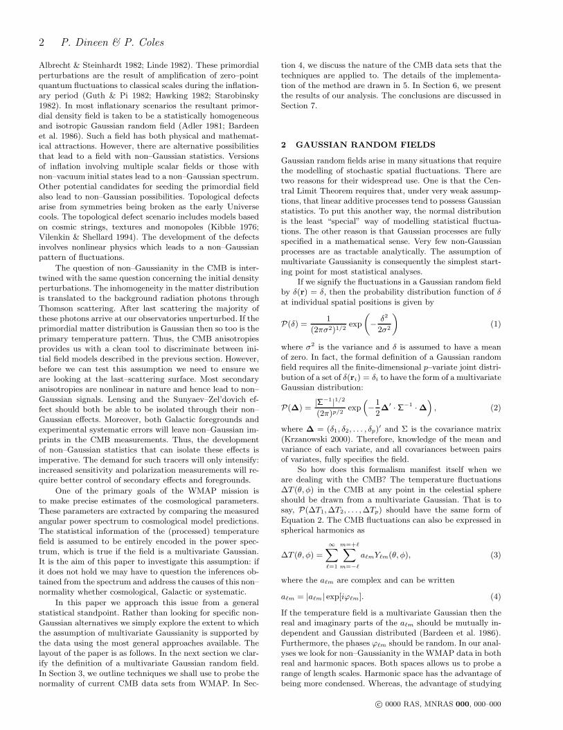
Figure 1. Skewness results from the foreground–cleaned assem-bly maps. (Top left) Q1 assembly map, (top right) Q2 assemblymap, (2nd from top, left) V 1 assembly map, (2nd from top, right)V 2 assembly map, (3rd from top, left) W1 assembly map, (3rdfrom top, right) W2 assembly map, (bottom, left) W3 assemblymap, and (bottom, right) W4 assembly map.

play the results for ∆T1 to increase clarity, although unsur-prising, the corresponding plots for ∆T2 resemble those for∆T1.

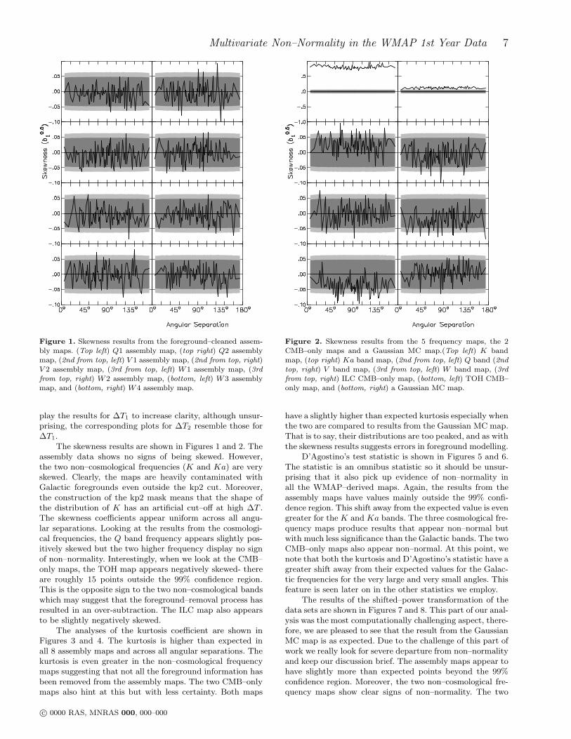
The skewness results are shown in Figures 1 and 2. Theassembly data shows no signs of being skewed. However,the two non–cosmological frequencies (K and Ka) are veryskewed. Clearly, the maps are heavily contaminated withGalactic foregrounds even outside the kp2 cut. Moreover,the construction of the kp2 mask means that the shape ofthe distribution of K has an artificial cut–off at high ∆T .The skewness coefficients appear uniform across all angu-lar separations. Looking at the results from the cosmologi-cal frequencies, the Q band frequency appears slightly pos-itively skewed but the two higher frequency display no signof non–normality. Interestingly, when we look at the CMB–only maps, the TOH map appears negatively skewed- thereare roughly 15 points outside the 99% confidence region.This is the opposite sign to the two non–cosmological bandswhich may suggest that the foreground–removal process hasresulted in an over-subtraction. The ILC map also appearsto be slightly negatively skewed.

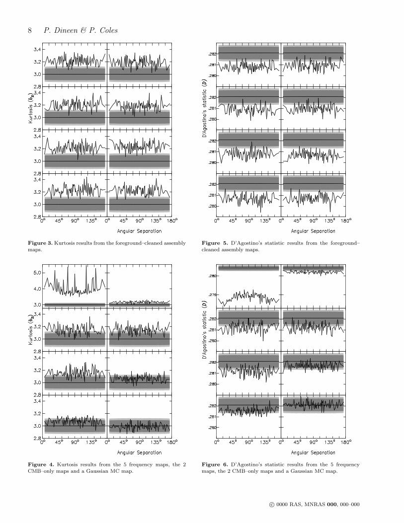
The analyses of the kurtosis coefficient are shown inFigures 3 and 4. The kurtosis is higher than expected inall 8 assembly maps and across all angular separations. Thekurtosis is even greater in the non–cosmological frequencymaps suggesting that not all the foreground information hasbeen removed from the assembly maps. The two CMB–onlymaps also hint at this but with less certainty. Both maps

Figure 2. Skewness results from the 5 frequency maps, the 2CMB–only maps and a Gaussian MC map.(Top left) K bandmap, (top right) Ka band map, (2nd from top, left) Q band (2ndtop, right) V band map, (3rd from top, left) W band map, (3rdfrom top, right) ILC CMB–only map, (bottom, left) TOH CMB–only map, and (bottom, right) a Gaussian MC map.

have a slightly higher than expected kurtosis especially whenthe two are compared to results from the Gaussian MC map.That is to say, their distributions are too peaked, and as withthe skewness results suggests errors in foreground modelling.

D’Agostino’s test statistic is shown in Figures 5 and 6.The statistic is an omnibus statistic so it should be unsur-prising that it also pick up evidence of non–normality inall the WMAP–derived maps. Again, the results from theassembly maps have values mainly outside the 99% confi-dence region. This shift away from the expected value is evengreater for the K and Ka bands. The three cosmological fre-quency maps produce results that appear non–normal butwith much less significance than the Galactic bands. The twoCMB–only maps also appear non–normal. At this point, wenote that both the kurtosis and D’Agostino’s statistic have agreater shift away from their expected values for the Galac-tic frequencies for the very large and very small angles. Thisfeature is seen later on in the other statistics we employ.

The results of the shifted–power transformation of thedata sets are shown in Figures 7 and 8. This part of our anal-ysis was the most computationally challenging aspect, there-fore, we are pleased to see that the result from the GaussianMC map is as expected. Due to the challenge of this part ofwork we really look for severe departure from non–normalityand keep our discussion brief. The assembly maps appear tohave slightly more than expected points beyond the 99%confidence region. Moreover, the two non–cosmological fre-quency maps show clear signs of non–normality. The two

c© 0000 RAS, MNRAS 000, 000–000


Figure 3. Kurtosis results from the foreground–cleaned assemblymaps.

Figure 4. Kurtosis results from the 5 frequency maps, the 2CMB–only maps and a Gaussian MC map.

Figure 5. D’Agostino’s statistic results from the foreground–cleaned assembly maps.

Figure 6. D’Agostino’s statistic results from the 5 frequencymaps, the 2 CMB–only maps and a Gaussian MC map.

c© 0000 RAS, MNRAS 000, 000–000


Figure 7. Univariate transformation results from theforeground–cleaned assembly maps.

CMB–only maps also show signs of non–normality- the TOHmap result appearing to have departed furthest from nor-mality.

6.1.2 Joint normality results

Our bivariate analysis results are shown in Figures 9-14. Thebivariate skewness statistics (nb12/6) calculated from the 16maps are shown in Figures 9 and 10. The statistic appears tobe abnormal for three of the assembly maps- Q1, W 2 andW 4. Some of the other assembly maps have two or threepoints outside the 99% confidence region but visually theresults do not look too unusual. Once again, the two non–cosmological frequencies have results that strongly indicatenon–normality. This non–normality is still evident in the Qand V band. The two CMB maps also have a higher thanexpected number of points above the 99% confidence region.It would appear that the bivariate skewness results mimictheir univariate counterparts.

The bivariate kurtosis results are displayed in Figures11 and 12. As with the skewness results, bivariate kurtosisseem similar to their univariate equivalent. Nevertheless, inthe case of the assembly maps, the shift away from the ex-pected value is even greater than for the univariate results.As before, the Galactic frequency maps are clearly found tobe non–normal. The higher value than expected value of thebivariate kurtosis persists in the foreground–cleaned CMBmaps

The bivariate power transformation is shown in Figures13 and 14. The assembly results do not look entirely consis-tent with being drawn from a χ2

2 distribution. Five of the

Figure 8. Univariate transformation results from the 5 frequencymaps, the 2 CMB–only maps and a Gaussian MC map.

Figure 9. Bivariate skewness results from the foreground–cleaned assembly maps.

c© 0000 RAS, MNRAS 000, 000–000


Figure 10. Bivariate skewness results from the 5 frequency maps,the 2 CMB–only maps and a Gaussian MC map.

Figure 11. Bivariate kurtosis results from the foreground–cleaned assembly maps.

Figure 12. Bivariate kurtosis results from the 5 frequency maps,the 2 CMB–only maps and a Gaussian MC map.

assembly maps produce results with 5 or more points out-side the 99% confidence region. Saying that, our GaussianMC map has four points outside this region, which makesit hard to draw definite conclusions. This is certainly nottrue for the two Galactic frequency bands that are clearlyinconsistent with normality. The two CMB–only maps alsoappear to have an extremely high number of points beyondthe 99% confidence region.

6.1.3 Linearity results

Lastly, in this subsection, we assess the linearity of the data.We tried adding separately three non–linear terms to ourlinear model of the data (as described in 5). However, allthree terms were found to be unnecessary descriptors forthe data from all of the maps bar the heavily contaminatedK band map. This is reassuring as it tells us that the angularpower spectrum supplies reliable information about the datasets. We plot in Figures 15 and 16 the results for additionof the z2j non–linear term. Curiously, the non–linearity seenin the K band map is seen at the largest and very smallestangular separations. As has already been noted, this trendis seen in other statistics that we employ.

6.2 Harmonic space

6.2.1 Marginal normality results

The results of applying the skewness, kurtosis andD’Agostino’s statistics are shown in Figures 17, 18 and 19,

c© 0000 RAS, MNRAS 000, 000–000


Figure 13.Bivariate transformation results from the foreground–cleaned assembly maps..

Figure 14. Bivariate transformation results from the 5 frequencymaps, the 2 CMB–only maps and a Gaussian MC map.

Figure 15. Linear regression results from the foreground–cleanedassembly maps.

Figure 16. Linear regression results from the 5 frequency maps,the 2 CMB–only maps and a Gaussian MC map.

c© 0000 RAS, MNRAS 000, 000–000


Figure 17. Skewness results from the aℓm of the 2 CMB–onlymaps and a Gaussian MC map. (Top left) ILC CMB–only map,(top right) TOH CMB–only map and (bottom) a Gaussian MCmap

Figure 18. Kurtosis results from the aℓm of the 2 CMB–onlymaps and a Gaussian MC map.

respectively. The results from the ILC map appear consis-tent with normality. However, all three statistic behave un-usually for the TOH map on scales smaller than ℓ ∼ 400,.This is particularly true of the kurtosis coefficient where thenon–normality is most evident. It would be interesting torelate this non–normality to that already seen in real space.This could hopefully give us a better handle on the sourceof the non–Gaussianity (whether Galactic or cosmological).The univariate transformation results are shown for com-pleteness in Figure 20. However, the method appears unre-liable as the Gaussian MC map results are inconsistent withbeing drawn from a χ2

1 distributions. We feel this unreliabil-ity is due to the small values of n that make the minimizedfunction shape more complex.

6.2.2 Joint normality results

The application of our bivariate skewness and kurtosisstatistics are shown in Figures 21 and 22. Once again, theILC map behaviour corresponds to that of the GaussianMC map. However, the TOH map shows clear signs of non–normality. The non–normality is displayed from larger scales

Figure 19. D’Agostino’s statistic results from the aℓm of the 2CMB–only maps and a Gaussian MC map.

Figure 20. Univariate transformation results from the aℓm ofthe 2 CMB–only maps and a Gaussian MC map.

than the univariate counterparts. That is to say, the distri-bution of the alms appears unusual at scales greater thanℓ = 300. The results from the multivariate power transfor-mations using harmonic space data are shown in Figure 23.Looking at the results from the ILC and Gaussian MC maps,it appears that we are failing to find the true global min-imum. As discussed earlier, finding a local minimum willresult in an underestimate of the value of χ2

2. Therefore,we are not too concerned about this as failure to find globalminima since it failure does not result in false claims of non–Gaussianity. Intriguingly, the shape of the line for the TOHmap does not match those of the other two maps. If we arefailing to find the global minima then the we would expecta larger number of points to be beyond the 99% confidenceregion if we corrected this failure. Equally, the result mayreflect that the distributions extracted from the TOH mapsmake finding the global minimum easier because they are,to some extent, smoother.

6.2.3 Linearity results

In our analysis of the linearity of the harmonic space vari-ates, we do not find any evidence of non–linearity. This was

c© 0000 RAS, MNRAS 000, 000–000


Figure 21. Bivariate skewness results from the aℓm of the 2CMB–only maps and a Gaussian MC map.

Figure 22. Bivariate kurtosis results from the aℓm of the 2 CMB–only maps and a Gaussian MC map.

Figure 23. Bivariate transformation results from the aℓm of the2 CMB–only maps and a Gaussian MC map.

Figure 24. Linear regression results from the aℓm of the 2 CMB–only maps and a Gaussian MC map.

also the case when we looked at the real space temperaturepairs. To illustrate this, we display in Figure 24 the resultsfrom the addition of the z2j non–linear term .

6.3 Other results

In light of the positive detections of non–normality, it isobviously important to gain some insight into its cause. Inthe Introduction, we stated that the distributions resultingfrom the various sources of non–Gaussianity are poorly un-derstood. Nevertheless, we can reduce the influence of pos-sible contaminants. In particular, by applying a more severemask to the data we should be able to observe regions ofthe CMB–sky where there is less Galactic contamination.We looked at the assembly data with the more severe kp0mask applied. Our techniques produce identical results tothose obtained from the kp2 mask: the skewness is consis-tent with normality; the kurtosis is inconsistent (∼ 3.2);D’Agostino’s statistic is inconsistent (ranging from 0.280 to0.281); and the bivariate kurtosis is inconsistent (∼ 8.5).This suggests that Galactic effects may not be causing thenon–normality we measure. However, we should be wary ofjumping to the conclusion that the signal is cosmological inorigin. Over subtraction, residual inhomogeneous noise, orother systematic effects may be the problem.

Another pertinent question is whether the detectednon–normality is associated with previous claims of non–Gaussianity. Eriksen et al. (2004) find an asymmetry be-tween the northern and southern Galactic hemispheres, withthe northern portion appearing devoid of large–scale struc-ture. Our techniques in real space allow us to localize re-gions of the sky. We apply our statistic to the northernand southern parts of the W 1 assembly map. We find thatthe kurtosis, D’Agostino’s and bivariate kurtosis statisticsshow identical signs of non–normality on both hemispheres.This suggests that the non–normality is symmetric aboutthe Galactic plane. Moreover, this also rules out the non–normality being associated with a localised ’cold–spot’ asdetected by wavelet techniques (McEwen et al. 2005; Vielvaet al. 2004).

c© 0000 RAS, MNRAS 000, 000–000


7 CONCLUSION

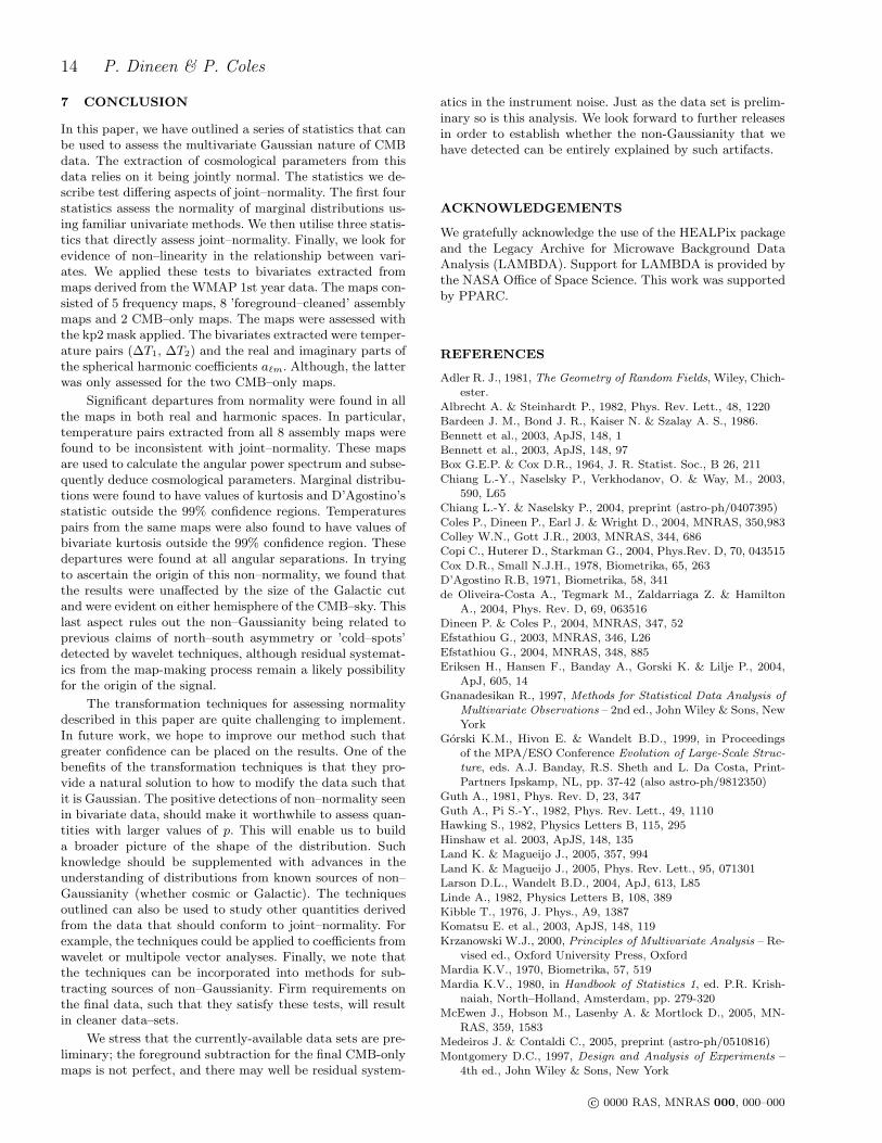
In this paper, we have outlined a series of statistics that canbe used to assess the multivariate Gaussian nature of CMBdata. The extraction of cosmological parameters from thisdata relies on it being jointly normal. The statistics we de-scribe test differing aspects of joint–normality. The first fourstatistics assess the normality of marginal distributions us-ing familiar univariate methods. We then utilise three statis-tics that directly assess joint–normality. Finally, we look forevidence of non–linearity in the relationship between vari-ates. We applied these tests to bivariates extracted frommaps derived from the WMAP 1st year data. The maps con-sisted of 5 frequency maps, 8 ’foreground–cleaned’ assemblymaps and 2 CMB–only maps. The maps were assessed withthe kp2 mask applied. The bivariates extracted were temper-ature pairs (∆T1, ∆T2) and the real and imaginary parts ofthe spherical harmonic coefficients aℓm. Although, the latterwas only assessed for the two CMB–only maps.

Significant departures from normality were found in allthe maps in both real and harmonic spaces. In particular,temperature pairs extracted from all 8 assembly maps werefound to be inconsistent with joint–normality. These mapsare used to calculate the angular power spectrum and subse-quently deduce cosmological parameters. Marginal distribu-tions were found to have values of kurtosis and D’Agostino’sstatistic outside the 99% confidence regions. Temperaturespairs from the same maps were also found to have values ofbivariate kurtosis outside the 99% confidence region. Thesedepartures were found at all angular separations. In tryingto ascertain the origin of this non–normality, we found thatthe results were unaffected by the size of the Galactic cutand were evident on either hemisphere of the CMB–sky. Thislast aspect rules out the non–Gaussianity being related toprevious claims of north–south asymmetry or ’cold–spots’detected by wavelet techniques, although residual systemat-ics from the map-making process remain a likely possibilityfor the origin of the signal.

The transformation techniques for assessing normalitydescribed in this paper are quite challenging to implement.In future work, we hope to improve our method such thatgreater confidence can be placed on the results. One of thebenefits of the transformation techniques is that they pro-vide a natural solution to how to modify the data such thatit is Gaussian. The positive detections of non–normality seenin bivariate data, should make it worthwhile to assess quan-tities with larger values of p. This will enable us to builda broader picture of the shape of the distribution. Suchknowledge should be supplemented with advances in theunderstanding of distributions from known sources of non–Gaussianity (whether cosmic or Galactic). The techniquesoutlined can also be used to study other quantities derivedfrom the data that should conform to joint–normality. Forexample, the techniques could be applied to coefficients fromwavelet or multipole vector analyses. Finally, we note thatthe techniques can be incorporated into methods for sub-tracting sources of non–Gaussianity. Firm requirements onthe final data, such that they satisfy these tests, will resultin cleaner data–sets.

We stress that the currently-available data sets are pre-liminary; the foreground subtraction for the final CMB-onlymaps is not perfect, and there may well be residual system-

atics in the instrument noise. Just as the data set is prelim-inary so is this analysis. We look forward to further releasesin order to establish whether the non-Gaussianity that wehave detected can be entirely explained by such artifacts.

ACKNOWLEDGEMENTS

We gratefully acknowledge the use of the HEALPix packageand the Legacy Archive for Microwave Background DataAnalysis (LAMBDA). Support for LAMBDA is provided bythe NASA Office of Space Science. This work was supportedby PPARC.

REFERENCES

Adler R. J., 1981, The Geometry of Random Fields, Wiley, Chich-ester.

Albrecht A. & Steinhardt P., 1982, Phys. Rev. Lett., 48, 1220Bardeen J. M., Bond J. R., Kaiser N. & Szalay A. S., 1986.

Bennett et al., 2003, ApJS, 148, 1Bennett et al., 2003, ApJS, 148, 97Box G.E.P. & Cox D.R., 1964, J. R. Statist. Soc., B 26, 211

Chiang L.-Y., Naselsky P., Verkhodanov, O. & Way, M., 2003,590, L65

Chiang L.-Y. & Naselsky P., 2004, preprint (astro-ph/0407395)

Coles P., Dineen P., Earl J. & Wright D., 2004, MNRAS, 350,983Colley W.N., Gott J.R., 2003, MNRAS, 344, 686Copi C., Huterer D., Starkman G., 2004, Phys.Rev. D, 70, 043515

Cox D.R., Small N.J.H., 1978, Biometrika, 65, 263D’Agostino R.B, 1971, Biometrika, 58, 341

de Oliveira-Costa A., Tegmark M., Zaldarriaga Z. & HamiltonA., 2004, Phys. Rev. D, 69, 063516

Dineen P. & Coles P., 2004, MNRAS, 347, 52Efstathiou G., 2003, MNRAS, 346, L26

Efstathiou G., 2004, MNRAS, 348, 885Eriksen H., Hansen F., Banday A., Gorski K. & Lilje P., 2004,

ApJ, 605, 14

Gnanadesikan R., 1997, Methods for Statistical Data Analysis of

Multivariate Observations – 2nd ed., John Wiley & Sons, NewYork

Gorski K.M., Hivon E. & Wandelt B.D., 1999, in Proceedingsof the MPA/ESO Conference Evolution of Large-Scale Struc-

ture, eds. A.J. Banday, R.S. Sheth and L. Da Costa, Print-Partners Ipskamp, NL, pp. 37-42 (also astro-ph/9812350)

Guth A., 1981, Phys. Rev. D, 23, 347Guth A., Pi S.-Y., 1982, Phys. Rev. Lett., 49, 1110Hawking S., 1982, Physics Letters B, 115, 295

Hinshaw et al. 2003, ApJS, 148, 135Land K. & Magueijo J., 2005, 357, 994

Land K. & Magueijo J., 2005, Phys. Rev. Lett., 95, 071301Larson D.L., Wandelt B.D., 2004, ApJ, 613, L85

Linde A., 1982, Physics Letters B, 108, 389Kibble T., 1976, J. Phys., A9, 1387Komatsu E. et al., 2003, ApJS, 148, 119

Krzanowski W.J., 2000, Principles of Multivariate Analysis – Re-vised ed., Oxford University Press, Oxford

Mardia K.V., 1970, Biometrika, 57, 519

Mardia K.V., 1980, in Handbook of Statistics 1, ed. P.R. Krish-naiah, North–Holland, Amsterdam, pp. 279-320

McEwen J., Hobson M., Lasenby A. & Mortlock D., 2005, MN-RAS, 359, 1583

Medeiros J. & Contaldi C., 2005, preprint (astro-ph/0510816)

Montgomery D.C., 1997, Design and Analysis of Experiments –4th ed., John Wiley & Sons, New York

c© 0000 RAS, MNRAS 000, 000–000


Naselsky P., Doroshkevich A. & Verkhodanov O., 2003, ApJ ,

599, L53Park C.-G., 2004, MNRAS, 349, 313Press W., Flannery B., Teukolsky S. & Vetterling W., 1992, Nu-

merical Recipes in C: The Art of Scientific Computing – 2nded., Cambridge University Press, Cambridge

Stannard A. & Coles P., 2005, MNRAS, 364, 929Starobinsky A., 1982, Physics Letters B, 117, 175Tegmark M., de Oliveira–Costa A. & Hamilton A., 2003,

Phys.Rev. D, 68, 123523Vielva P., Martinez–Gonzalez E., Barreiro R., Sanz J & Cayon

L., 2004, ApJ, 609, 22Vilenkin A. & Shellard E., 1994, Cosmic strings and other topo-

logical defects, Cambridge University Press, Cambridge

c© 0000 RAS, MNRAS 000, 000–000

multivariate non–normality in wmap 1st year data non–normality in the wmap 1st year data 3 in...

Documents