multivariate max-stable spatial processes · multivariate max-stable spatial processes by marc g....
TRANSCRIPT
Biometrika (2015), 102, 1, pp. 215–230 doi: 10.1093/biomet/asu066Printed in Great Britain Advance Access publication 11 February 2015
Multivariate max-stable spatial processes
BY MARC G. GENTON
CEMSE Division, King Abdullah University of Science and Technology, Thuwal 23955-6900,Saudi Arabia
SIMONE A. PADOAN
Department of Decision Sciences, Bocconi University of Milan, 20136 Milano, Italy
AND HUIYAN SANG
Department of Statistics, Texas A&M University, College Station, Texas 77843, U.S.A.
SUMMARY
Max-stable processes allow the spatial dependence of extremes to be modelled and quan-tified, so they are widely adopted in applications. For a better understanding of extremes, itmay be useful to study several variables simultaneously. To this end, we study the maxima ofindependent replicates of multivariate processes, both in the Gaussian and Student-t cases. Wedefine a Poisson process construction and introduce multivariate versions of the Smith Gaussianextreme-value, the Schlather extremal-Gaussian and extremal-t , and the Brown–Resnick mod-els. We develop inference for the models based on composite likelihoods. We present results ofMonte Carlo simulations and an application to daily maximum wind speed and wind gust.
Some key words: Composite likelihood; Cross-correlation; Extremal coefficient; Max-stable process; Multivariateanalysis; Random field; Spatial extreme.
1. INTRODUCTION
The statistical modelling of spatial extremes of natural processes is important in environmen-tal studies to understand the probability of events such as floods, heat waves, or hurricanes.Extreme events in space can be described by max-stable processes (de Haan & Ferreira, 2006),which extend the generalized extreme-value distribution. In a seminal unpublished University ofSurrey 1990 technical report, R. L. Smith, using the de Haan (1984) spectral representation, pro-posed a spatial max-stable model, named the Gaussian extreme-value process, whose dependencestructure is obtained using Gaussian densities. Schlather (2002) extended the de Haan formula-tion to random functions and proposed a model, named the extremal-Gaussian process. Anotherpopular spatial max-stable model is the Brown–Resnick process (Brown & Resnick, 1977;Kabluchko et al., 2009). The extremal-Gaussian max-stable model based on compact randomsets was introduced by Schlather (2002) and used by Davison & Gholamrezaee (2012). Spatio-temporal max-stable processes have been discussed by Kabluchko (2009), Davis et al. (2013) andHuser & Davison (2014). Asymptotically independent processes for modelling extreme valueswere discussed by de Haan & Zhou (2011), Wadsworth & Tawn (2012) and Padoan (2013a).
c© 2015 Biometrika Trust
at King A
bdullah University of Science and T
echnology on February 24, 2015http://biom
et.oxfordjournals.org/D
ownloaded from
216 M. G. GENTON, S. A. PADOAN AND H. SANG
Reviews of recent advances in the statistical modelling of spatial extremes are Davison et al.(2012), Cooley et al. (2012), Padoan (2013b), Ribatet (2013) and Davison & Huser (2015).
Although the aforementioned literature attests to vigorous research, it is limited to modelling asingle variable. In practice, however, multiple variables are often observed. For instance, rainfall,temperature and wind may be observed at many locations spread across a region. Each of thesevariables has its own spatial variation but also depends on the other variables. The aim of thispaper is to extend the theory and application of max-stable processes to the multivariate setting.Zhang & Smith (2004) investigated the behaviour of multivariate maxima of moving maximaprocesses, but these are not suitable for modelling spatial extremes. There is thus a need to extendmax-stable processes to the multivariate setting and to make them practically useful.
To fix notation, let I = {1, . . . , p} and K = {1, . . . , q} be sets of indices of variables andof spatial locations, respectively. Let N = pq, J = I × K be the Cartesian product and Jik ={( j, l) ∈ J\(i, k)}. We denote by {Yi (s)}s∈S a real-valued random process on S ⊆ R
d , with i ∈ N.Let Y (s)= {Y1(s), . . . , Yp(s)}T be a p-vector of processes observed in S and let {Y (m)(s)}m�1be independent copies of Y (s).
2. MAXIMA OF INDEPENDENT REPLICATES OF MULTIVARIATE PROCESSES
2·1. Gaussian case
For every n ∈ N, let {Yn(s)}s∈S be a p-dimensional Gaussian process that is second-orderstationary with a zero-mean vector function, unit variances, and a matrix-valued covariancefunction, �(h; n)= {ρi j (h; n)}i, j∈I , h ∈ R
d . Specifically, ρi j (h; n)= E{Yin(s) Y jn(s + h)} isthe spatial cross-correlation function between processes i and j , with i |= j , and h is the spatiallag between locations. When j = i , ρi i (h; n) is the correlation function of process i . If h = 0,then ρi i = 1 and ρi j represents the correlation between components. For simplicity of notation,we write ρi j (n) and ρi (h; n) for ρi j (0; n) and ρi i (h; n), respectively.
Let bn be a sequence such that (2π)1/2bn exp(b2n/2)∼ n as n → ∞ (Resnick, 1987, Ch. 1).
Assumption 1. Suppose that the dependence structure, �(h; n), of Yn(s) depends on n with
2b2n {ϒ −�(h; n)} →�(h), n → ∞,
where ϒ is a p × p matrix of ones and �(h) is a matrix-valued nonnegative function. Bythis, we mean that, for the correlation structure, the following constraints are fulfilled: 2b2
n{1 −ρi j (h; n)} → λ2
i j (h) as n → ∞, for all h ∈ Rd and for any i, j ∈ I , where λ2
i j (h) is a nonnega-
tive function. When j |= i and h = 0, 2b2n {1 − ρi j (n)} → λ2
i j , as n → ∞, where λ2i j ∈ [0,∞) is
assumed. When j = i and h = 0, then ρi (n)= 1 and λ2i = 0.
The quantity λ2i j measures the strength of the dependence among the variables in the limit,
λ2i (h) and λ2
i j (h) represent the limiting spatial inter-component and cross-component dependencefunctions. If Assumption 1 holds, then we derive the following generalization of the Husler–Reissmodel (Husler & Reiss, 1989; Kabluchko et al., 2009; Kabluchko, 2011).
PROPOSITION 1. For every n ∈ N, let {Y (m)n (s)}nm=1 be independent copies of Yn(s) and let
Mn(s)= {Min(s)}i∈I be the vector of pointwise maxima, where Min(s)= maxm=1,...,n{Y (m)in (s)},for all s ∈ S. Take Zn(s)= bn{Mn(s)− bn}. Then, Zn(s)→ Z(s) weakly as n → ∞ and{Z(s)}s∈S is a p-dimensional max-stable process with a finite dimensional distribution, for pos-itive values {zi (sk)}(i,k)∈J with sk ∈ S, equal to exp(−V [N ]
1···p[{zi (sk)}(i,k)∈J ]) where N = pq and
at King A
bdullah University of Science and T
echnology on February 24, 2015http://biom
et.oxfordjournals.org/D
ownloaded from

Multivariate max-stable spatial processes 217
V [N ]1···p[{zi (sk)}(i,k)∈J ] equals
∑(i,k)∈J
1
zi (sk)�N−1,�ik
⎛⎝[λi j (sk − sl)
2+ log
{z j (sl)/zi (sk)
}λi j (sk − sl)
]( j,l)∈Jik
⎞⎠ , (1)
where �N−1,�ikis the (N − 1)-dimensional Gaussian distribution function with mean zero and
partial correlation matrix, �ik , provided that this matrix is invertible.
The proof and the form of �ik are reported in the Supplementary Material. Here,V [N ]
1···p[{zi (sk)}(i,k)∈J ] is a multivariate exponent function; see de Haan & Ferreira (2006, Ch. 9)for a discussion of the univariate case. The superscript on V means that it is an exponent functionof N random components, that is, p variables observed at q sites. The subscript lists the vari-ables involved. The overall dependence among the p spatial variables is fully described by (1),which depends on the spatial cross-component dependence, λi j (sk − sl), the individual spatialdependence, λi (sk − sl), and the dependence between variables, λi j . We call the process Z(s)with exponent function (1) the multivariate Husler–Reiss process. In (1), if we set a commonthreshold, z, then the multivariate extremal coefficient is
θ[N ]1···p({sk − sl}k,l∈K )=
∑(i,k)∈J
�N−1,�ik
[{λi j (sk − sl)/2
}( j,l)∈Jik
].
In this case, 1 � θ[N ]1···p({sk − sl}k,l∈K )� N , where the lower bound represents the complete
dependence case, arising when all variables are totally dependent, whereas the upper bound rep-resents independence (Schlather & Tawn, 2003).
Since for a large number of variables and locations, θ [N ]1...p({sk − sl}k,l∈K ) may be difficult
to compute, interpret and represent graphically, we propose to use the following lower-orderextremal coefficients to summarize the dependence of multiple spatial extremes. Consider a pairof variables, (Zi , Z j ), i, j ∈ I (i |= j), observed at two sites separated by h ∈ R
d . A natural sum-mary of the spatial dependence between the extremes of two variables is the pairwise cross-component extremal coefficient, θ [2]
i j (h)= 2�{λi j (h)/2} ∈ [1, 2]. In general, θ [2]i j (h) |= θ [2]
j i (h),since λi j (h) |= λ j i (h), because ρi j (h) |= ρ j i (h). For a full understanding of the dependence,
θ[2]i j (h), θ
[2]j i (h), θ
[2]i (h), θ [2]
j (h) and θ [2]j i should be considered together. A richer measure that
simultaneously uses the information of λi j (h), λ j i (h), λi (h), λ j (h) and λi j is the quadruplewisespatial extremal cross-component coefficient,
θ[4]i j (h)=�3,�1
{λi (h)
2,λi j
2,λi j (h)
2
}+�3,�2
{λi (h)
2,λ j i (h)
2,λi j
2
}
+ �3,�3
{λ j (h)
2,λi j
2,λ j i (h)
2
}+�3,�4
{λ j (h)
2,λi j (h)
2,λi j
2
}∈ [1, 4]. (2)
This is derived from the distribution of {Zi (s), Z j (s), Zi (s + h), Z j (s + h)}, provided in theSupplementary Material with the matrices, �i (i = 1, . . . , 4). The coefficient in (2) satisfiesθ
[4]i j (h)= θ
[4]j i (h), and the pairwise coefficients, θ [2]
i j (h), θ[2]j i (h), θ
[2]i (h), θ [2]
j (h) and θ [2]i j are spe-
cial cases.
at King A
bdullah University of Science and T
echnology on February 24, 2015http://biom
et.oxfordjournals.org/D
ownloaded from

218 M. G. GENTON, S. A. PADOAN AND H. SANG
We can also consider (Zi , Z j , Zv) with i, j, v ∈ I (i |= j |= v), separated by h, h′, h′′ ∈ Rd ,
giving the triplewise spatial extremal cross-component coefficient,
θ[3]i jv(h, h′, h′′)=�2,�1
{λi j (h)
2,λiv(h′)
2
}+�2,�2
{λi j (h)
2,λ jv(h′′)
2
}(3)
+ �2,�3
{λiv(h′)
2,λ jv(h′′)
2
}∈ [1, 3].
This summarizes the extremal dependence for {Zi (s), Z j (s + h), Zv(s + h′)}. Although
θ[3]i jv(h, h′, h′′) is not invariant with respect to the order of the variables, it represents a com-
promise between complexity and interpretability.
2·2. Correlation models for the Gaussian case
The validity of result (1) depends on whether Assumption 1 is met. Such constraints are satis-fied by the class of multivariate Gaussian random fields with sufficiently smooth spatial isotropiccross-correlation functions for which, around h = 0,
ρi j (h; n)= 1 − cn λ2i j − cn ψ ‖h‖κ + o(c2
n), (4)
for a sequence of constants, cn , such that cn → 0 as n → ∞, where 0< κ � 2 is a smoothnessparameter, and ψ and λ2
i j , i, j ∈ I , are nonnegative constants. An example of a multivariate cor-relation model satisfying (4) is the class of power exponential correlation
ρ(h)≡ ρ(h;α, κ)= exp
{−(‖h‖α
)κ}(α > 0, 0< κ � 2),
where the parameters κ and α represent the smoothness and the scale of the spatial random field.The cross-correlation functions, with any i, j ∈ I and j |= i , are defined by ρi j (h)= ρ j i (h)=ρi jρ(h), which contains a factor ρi j that expresses the correlation between the variables. Con-sidering a correlation matrix,� = {ρi j }i, j∈I , among components, the overall dependence,�(h),emerges as a nonnegative definite correlation matrix. This correlation model is obtained as aproduct between the inter- and cross-correlations. It is therefore separable between the variablesand the spatial domain. It includes the exponential correlation, κ = 1, and the Gaussian correla-tion, κ = 2.
Define ρi j (h; n)= ρi j (n)ρ(cκn h), where ρi j (n)= 1 − cnλ2i j + o(cn) and ρ(cκn h)= 1 −
cn ψ ‖h‖κ + o(cn), for cn → 0 as n → ∞. Then, choosing cn = (2b2n)
−1, it follows that 2b2n
{1 − ρi j (h; n)} → λ2i j (h), where λ2
i j (h)= λ2i j + λ2(h) is the spatial cross-component depen-
dence function, with λi j the cross-component parameter and λ2(h)= (‖h‖/α)κ the spatialdependence function. With this correlation model, ψ = α−κ in (4) and ρi j (h)= ρ j i (h) so that
θ[2]i j (h)= θ
[2]j i (h), thus (2) simplifies to
θ[4]i j (h)= 4�3,�1
{λ(h)/2, λi j/2, λi j (h)/2
}. (5)
Although ρi j (h) is separable, the dependence structure of the limiting distribution is not. Indeed,(5) is not a product of two coefficients, one describing the spatial dependence and the other thedependence among variables. Further properties of (5) are reported next. Set h = ‖h‖. When thevariables are completely dependent, that is, λi j = 0, then λi j (h)= λ(h) and hence θ [4]
i j (0)= 1
and θ [4]i j (h)→ 2 as h → ∞. Thus, (5) behaves as the usual pairwise spatial coefficient. When
the variables are dependent, that is, 0<λi j <∞, then 1< θ [4]i j (h) < 4 for any h > 0 and it is
at King A
bdullah University of Science and T
echnology on February 24, 2015http://biom
et.oxfordjournals.org/D
ownloaded from
Multivariate max-stable spatial processes 219
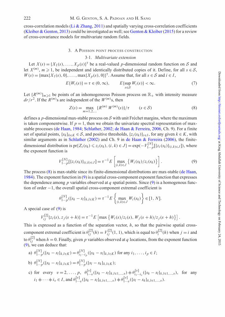
0 20 40 60 80 100 120
1·2
1·4
1·6
1·8
2·0
2·2
2·4
2·6(a) (b)
h
q ij[4] (h
)
q ij[4] (h
)
0 20 40 60 80 100 120
1·2
1·4
1·6
1·8
2·0
2·2
2·4
2·6
h
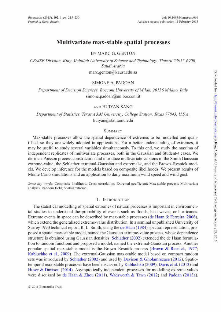
Fig. 1. Quadruplewise extremal coefficient functions of the bivariate Husler–Reissprocess with power exponential cross-correlation. (a): The curves from top to bot-tom correspond to 10 equally spaced values of α from 1 to 100 and fixed κ = 0·5;(b): the curves from bottom to top correspond to 10 equally spaced values of κ
from 0·5 to 2 and fixed α= 15. In both cases, λi j = 0·8 and h = ‖h‖.
1< θ [4]i j (0) < 2 if h = 0. Thus, (5) behaves like the usual pairwise cross-component coefficient.
When the variables are independent, that is, λi j = ∞, then θ [4]i j (0)= 2 if h = 0 and θ [4]
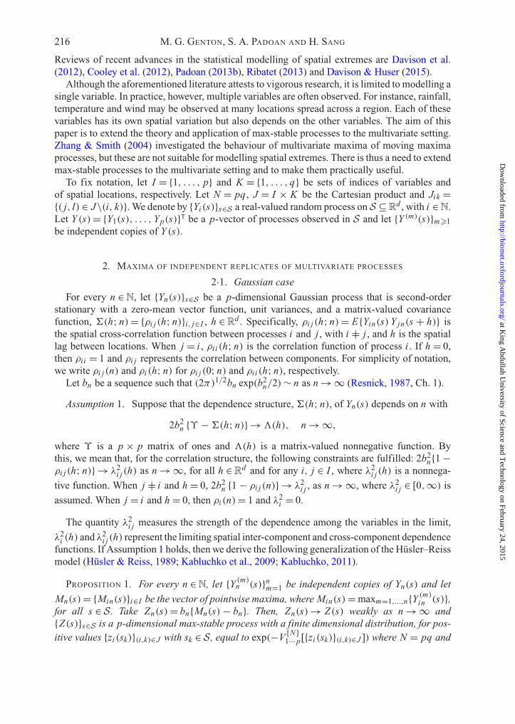
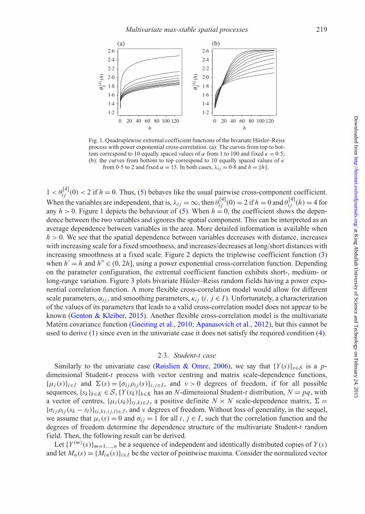
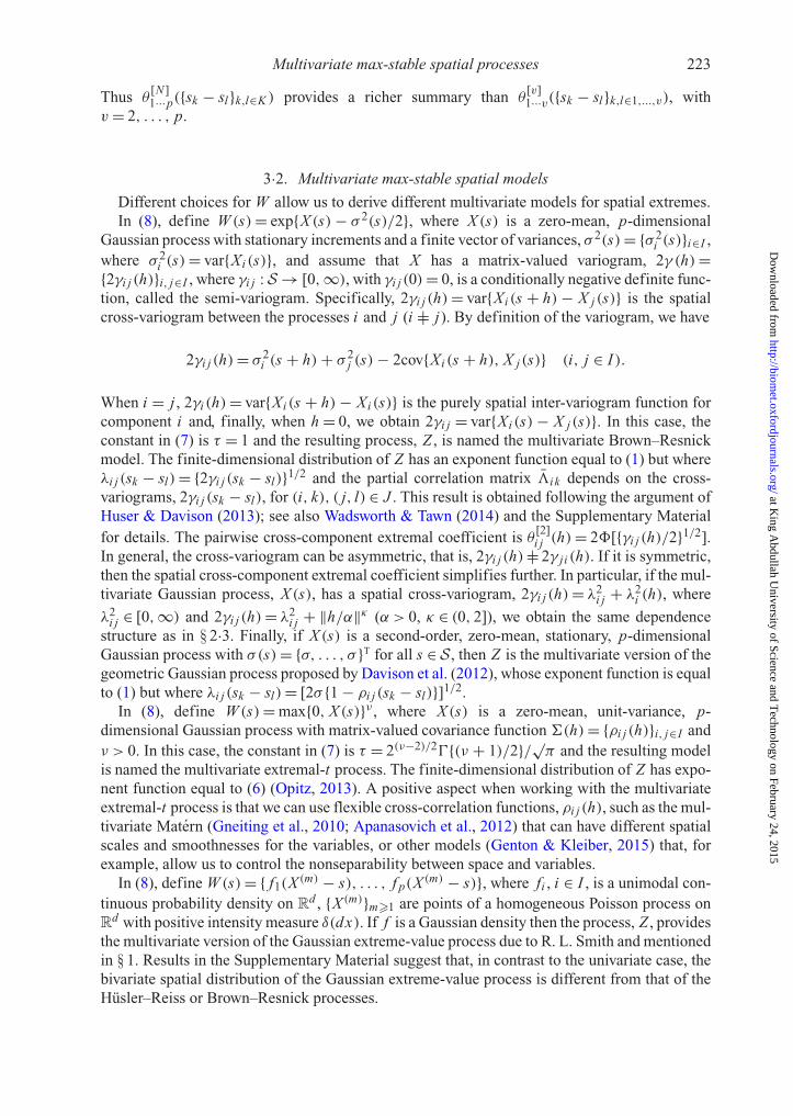
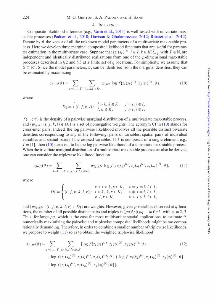
i j (h)= 4 forany h > 0. Figure 1 depicts the behaviour of (5). When h = 0, the coefficient shows the depen-dence between the two variables and ignores the spatial component. This can be interpreted as anaverage dependence between variables in the area. More detailed information is available whenh > 0. We see that the spatial dependence between variables decreases with distance, increaseswith increasing scale for a fixed smoothness, and increases/decreases at long/short distances withincreasing smoothness at a fixed scale. Figure 2 depicts the triplewise coefficient function (3)when h′ = h and h′′ ∈ (0, 2h], using a power exponential cross-correlation function. Dependingon the parameter configuration, the extremal coefficient function exhibits short-, medium- orlong-range variation. Figure 3 plots bivariate Husler–Reiss random fields having a power expo-nential correlation function. A more flexible cross-correlation model would allow for differentscale parameters, αi j , and smoothing parameters, κi j (i, j ∈ I ). Unfortunately, a characterizationof the values of its parameters that leads to a valid cross-correlation model does not appear to beknown (Genton & Kleiber, 2015). Another flexible cross-correlation model is the multivariateMatern covariance function (Gneiting et al., 2010; Apanasovich et al., 2012), but this cannot beused to derive (1) since even in the univariate case it does not satisfy the required condition (4).
2·3. Student-t case
Similarly to the univariate case (Røislien & Omre, 2006), we say that {Y (s)}s∈S is a p-dimensional Student-t process with vector centring and matrix scale-dependence functions,{μi (s)}i∈I and �(s)= {σi jρi j (s)}i, j∈I , and ν > 0 degrees of freedom, if for all possiblesequences, {sk}k∈K ∈ S, {Y (sk)}k∈K has an N -dimensional Student-t distribution, N = pq, witha vector of centres, {μi (sk)}(i,k)∈J , a positive definite N × N scale-dependence matrix, � ={σi jρi j (sk − sl)}(i,k),( j,l)∈J , and ν degrees of freedom. Without loss of generality, in the sequel,we assume that μi (s)= 0 and σi j = 1 for all i, j ∈ I , such that the correlation function and thedegrees of freedom determine the dependence structure of the multivariate Student-t randomfield. Then, the following result can be derived.
Let {Y (m)(s)}m=1,...,n be a sequence of independent and identically distributed copies of Y (s)and let Mn(s)= {Min(s)}i∈I be the vector of pointwise maxima. Consider the normalized vector
at King A
bdullah University of Science and T
echnology on February 24, 2015http://biom
et.oxfordjournals.org/D
ownloaded from
220 M. G. GENTON, S. A. PADOAN AND H. SANG
20 60 1000
50
100
150
200
250
a = 15, k = 0·3, l = 0·3
h'
1·65 1·7 1·75
1·8
1·85
1·9
20 60 1000
50
100
150
200
250
a = 15, k = 0·3, l = 1
1·8 1·85 1·9
1·95
2
20 60 100
20 60 100 20 60 100 20 60 100
20 60 100 20 60 100 20 60 100
0
50
100
150
200
250
a = 15, k = 0·3, l = 1·5
a = 15, k = 1·8, l = 0·3 a = 15, k = 1·8, l = 1 a = 15, k = 1·8, l = 1·5
a = 30, k = 1·8, l = 0·3 a = 30, k = 1·8, l = 1 a = 30, k = 1·8, l = 1·5
2·14 2·16 2·18
2·2 2·22
2·24 2·26
0
50
100
150
200
250
h'
1·8 2 2·2 2·4
2·6 2·8
0
50
100
150
200
250
2 2·4 2·6
2·8
0
50
100
150
200
250 2·3 2·5 2·6
2·7 2·8
2·9
0
50
100
150
200
250
h
h'
1·6 2 2·2
2·4
2·6
2·8
0
50
100
150
200
250
h
1·7 1·9 2
2·1
2·2 2·3
2·4
2·5 2·6
2·7 2·8
0
50
100
150
200
250
h
2 2·1
2·3 2·4 2·5
2·6
2·7
2·8
2·9
1
1·5
2
2·5
3
Fig. 2. Triplewise extremal coefficient functions of the trivariate Husler–Reiss process with power exponential
cross-correlation. Reported is θ [3]i jv(h, h, h′)with h = ‖h‖, h′ ∈ (0, 2h], different parameter values and λi j = λiv =
λ jv = λ. Extremal coefficients with short, medium and long range are reported from the top to the bottom panels.
of pointwise maxima, Zn(s)= Mn(s)/an(s), where an(s) > 0 is an appropriate vector of normal-izing functions. Then, Zn(s)→ Z(s) weakly as n → ∞, where Z(s) is a p-dimensional max-stable process with a finite-dimensional distribution that depends on the exponent function
∑(i,k)∈J
1
zi (sk)TN−1,�ik ,ν+1
⎧⎨⎩⎛⎝{ ν + 1
1 − ρ2i j (sk − sl)
}1/2 [{z j (sl)
zi (sk)
}1/ν
− ρi j (sk − sl)
]⎞⎠( j,l)∈Jik
⎫⎬⎭ , (6)
at King A
bdullah University of Science and T
echnology on February 24, 2015http://biom
et.oxfordjournals.org/D
ownloaded from

Multivariate max-stable spatial processes 221
0 20 40 60 800
20
40
60
80
0
20
40
60
80
0
20
40
60
80
0
20
40
60
80
s 2s 2
s 2
Z1(s); a = 15,k = 0·3
0 20 40 60 80
Z2(s); l12 = 0·3
0 20 40 60 80
Z2(s); l12 = 1
0 20 40 60 80
0 20 40 60 80 0 20 40 60 80 0 20 40 60 80 0 20 40 60 80
0 20 40 60 80 0 20 40 60 80 0 20 40 60 80 0 20 40 60 80
Z2(s); l12 = 1·5
0
20
40
60
80
Z1(s); a = 15,k = 1·8
0
20
40
60
80
0
20
40
60
80
0
20
40
60
80
0
20
40
60
80
0
20
40
60
80
0
20
40
60
80
0
20
40
60
80
s1 s1 s1 s1
Z1(s); a = 30,k = 1·8
−2·5 −1·5 −0·5 0·5 1·5 2·5 3·5 4·5 5·5
Fig. 3. Simulated bivariate Husler–Reiss max-stable random fields having a power exponential cross-correlation function at a mesh grid of 60 × 60 on [0, 100]2. Margins are on the standard Gumbel scale.
where TN−1,�ik ,ν+1 is an (N − 1)-dimensional Student-t cumulative distribution function with
zero centres, partial correlation matrix �ik , and ν + 1 degrees of freedom; see the SupplementaryMaterial for details. We call the process Z(s) with distribution (6) the multivariate extremal-tprocess; for the univariate case, see Nikoloulopoulos et al. (2009), Davison et al. (2012), andOpitz (2013). In this case, the spatial extremal cross-component coefficient is
θ[N ]1···p({sk − sl}k,l∈K )=
∑(i,k)∈J
TN−1,�ik ,ν+1
⎧⎨⎩([
(ν + 1){1 − ρi j (sk − sl)}1 + ρi j (sk − sl)
]1/2)( j,l)∈Jik
⎫⎬⎭ .
Triplewise and quadruplewise extremal coefficient functions similar to those in (2) and (3) canbe derived. The pairwise spatial extremal cross-component coefficient is
θ[2]i j (h)= 2Tν+1
([(ν + 1){1 − ρi j (h)}/{1 + ρi j (h)}
]1/2),
where Tν+1 is a univariate Student-t cumulative distribution function with ν + 1 degrees offreedom, h ∈ R
d . The benefit of working with the multivariate extremal-t process rather thanwith the Husler–Reiss model is that we can use the multivariate Matern covariance function(Gneiting et al., 2010; Apanasovich et al., 2012). Nonseparable cross-correlation models can beconstructed using latent dimensions as proposed by Apanasovich & Genton (2010). Asymmetric
at King A
bdullah University of Science and T
echnology on February 24, 2015http://biom
et.oxfordjournals.org/D
ownloaded from
222 M. G. GENTON, S. A. PADOAN AND H. SANG
cross-correlation models (Li & Zhang, 2011) and spatially varying cross-correlation coefficients(Kleiber & Genton, 2013) could be investigated as well; see Genton & Kleiber (2015) for a reviewof cross-covariance models for multivariate random fields.
3. A POISSON POINT PROCESS CONSTRUCTION
3·1. Multivariate extension
Let X (s)= {X1(s), . . . , X p(s)}T be a real-valued p-dimensional random function on S andlet X (m), m � 1, be independent and identically distributed copies of it. Define, for all s ∈ S,W (s)= {max{X1(s), 0}, . . . ,max{X p(s), 0}}T. Assume that, for all s ∈ S and i ∈ I ,
E{Wi (s)} = τ ∈ (0,∞), E{sups∈S
Wi (s)}<∞. (7)
Let {R(m)}m�1 be points of an inhomogeneous Poisson process on R+ with intensity measuredr/r2. If the R(m)s are independent of the W (m)s, then
Z(s)= maxm=1,2,...
{R(m) W (m)(s)}/τ (s ∈ S) (8)
defines a p-dimensional max-stable process on S with unit Frechet margins, where the maximumis taken componentwise. If p = 1, then we obtain the univariate spectral representation of max-stable processes (de Haan, 1984; Schlather, 2002; de Haan & Ferreira, 2006, Ch. 9). For a finiteset of spatial points, {sk}k∈K ∈ S, and positive thresholds, {zi (sk)}i∈I , for any given k ∈ K , withsimilar arguments as in Schlather (2002) and Ch. 9 in de Haan & Ferreira (2006), the finite-dimensional distribution is pr{Zi (sk)� zi (sk), (i, k) ∈ J } = exp(−V [N ]
1···p[{zi (sk)}(i,k)∈J ]), wherethe exponent function is
V [N ]1···p[{zi (sk)}(i,k)∈J ] = τ−1 E
[max(i,k)∈J
{Wi (sk)/zi (sk)
}]. (9)
The process (8) is max-stable since its finite-dimensional distributions are max-stable (de Haan,1984). The exponent function in (9) is a spatial cross-component exponent function that expressesthe dependence among p variables observed at q spatial points. Since (9) is a homogenous func-tion of order −1, the overall spatial cross-component extremal coefficient is
θ[N ]1···p({sk − sl}k,l∈K )= τ−1 E
{max(i,k)∈J
Wi (sk)
}∈ [1, N ].
A special case of (9) is
V [2]i j {zi (s), z j (s + h)} = τ−1 E
[max
{Wi (s)/zi (s),W j (s + h)/z j (s + h)
}].
This is expressed as a function of the separation vector, h, so that the pairwise spatial cross-
component extremal coefficient is θ [2]i j (h)= V [2]
i j (1, 1), which is equal to θ [2]i (h) when j = i and
to θ [2]i j when h = 0. Finally, given p variables observed at q locations, from the exponent function
(9), we can deduce that:
a) θ [N ]1···p({sk − sl}k,l∈K )= θ
[N ]i1···i p
({sk − sl}k,l∈K ) for any i1, . . . , i p ∈ I ;
b) θ [N ]1···p({sk − sl}k,l∈K )= θ
[N ]1···p({sl − sk}k,l∈K );
c) for every v = 2, . . . , p, θ[v]1···v({sk − sl}k,l∈1,...,v) |= θ [v]
i1···iv ({sk − sl}k,l∈1,...,v), for any
i1 |= · · · |= iv ∈ I , and θ [v]1···v({sk − sl}k,l∈1,...,v) |= θ [v]
1···v({sl − sk}k,l∈1,...,v).
at King A
bdullah University of Science and T
echnology on February 24, 2015http://biom
et.oxfordjournals.org/D
ownloaded from
Multivariate max-stable spatial processes 223
Thus θ[N ]1···p({sk − sl}k,l∈K ) provides a richer summary than θ
[v]1···v({sk − sl}k,l∈1,...,v), with
v = 2, . . . , p.
3·2. Multivariate max-stable spatial models
Different choices for W allow us to derive different multivariate models for spatial extremes.In (8), define W (s)= exp{X (s)− σ 2(s)/2}, where X (s) is a zero-mean, p-dimensional
Gaussian process with stationary increments and a finite vector of variances, σ 2(s)= {σ 2i (s)}i∈I ,
where σ 2i (s)= var{Xi (s)}, and assume that X has a matrix-valued variogram, 2γ (h)=
{2γi j (h)}i, j∈I , where γi j : S → [0,∞), with γi j (0)= 0, is a conditionally negative definite func-tion, called the semi-variogram. Specifically, 2γi j (h)= var{Xi (s + h)− X j (s)} is the spatialcross-variogram between the processes i and j (i |= j). By definition of the variogram, we have
2γi j (h)= σ 2i (s + h)+ σ 2
j (s)− 2cov{Xi (s + h), X j (s)} (i, j ∈ I ).
When i = j , 2γi (h)= var{Xi (s + h)− Xi (s)} is the purely spatial inter-variogram function forcomponent i and, finally, when h = 0, we obtain 2γi j = var{Xi (s)− X j (s)}. In this case, theconstant in (7) is τ = 1 and the resulting process, Z , is named the multivariate Brown–Resnickmodel. The finite-dimensional distribution of Z has an exponent function equal to (1) but whereλi j (sk − sl)= {2γi j (sk − sl)}1/2 and the partial correlation matrix �ik depends on the cross-variograms, 2γi j (sk − sl), for (i, k), ( j, l) ∈ J . This result is obtained following the argument ofHuser & Davison (2013); see also Wadsworth & Tawn (2014) and the Supplementary Materialfor details. The pairwise cross-component extremal coefficient is θ [2]
i j (h)= 2�[{γi j (h)/2}1/2].In general, the cross-variogram can be asymmetric, that is, 2γi j (h) |= 2γ j i (h). If it is symmetric,then the spatial cross-component extremal coefficient simplifies further. In particular, if the mul-tivariate Gaussian process, X (s), has a spatial cross-variogram, 2γi j (h)= λ2
i j + λ2i (h), where
λ2i j ∈ [0,∞) and 2γi j (h)= λ2
i j + ‖h/α‖κ (α > 0, κ ∈ (0, 2]), we obtain the same dependencestructure as in § 2·3. Finally, if X (s) is a second-order, zero-mean, stationary, p-dimensionalGaussian process with σ(s)= {σ, . . . , σ }T for all s ∈ S, then Z is the multivariate version of thegeometric Gaussian process proposed by Davison et al. (2012), whose exponent function is equalto (1) but where λi j (sk − sl)= [2σ {1 − ρi j (sk − sl)}]1/2.
In (8), define W (s)= max{0, X (s)}ν , where X (s) is a zero-mean, unit-variance, p-dimensional Gaussian process with matrix-valued covariance function �(h)= {ρi j (h)}i, j∈I andν > 0. In this case, the constant in (7) is τ = 2(ν−2)/2�{(ν + 1)/2}/√π and the resulting modelis named the multivariate extremal-t process. The finite-dimensional distribution of Z has expo-nent function equal to (6) (Opitz, 2013). A positive aspect when working with the multivariateextremal-t process is that we can use flexible cross-correlation functions, ρi j (h), such as the mul-tivariate Matern (Gneiting et al., 2010; Apanasovich et al., 2012) that can have different spatialscales and smoothnesses for the variables, or other models (Genton & Kleiber, 2015) that, forexample, allow us to control the nonseparability between space and variables.
In (8), define W (s)= { f1(X (m) − s), . . . , f p(X (m) − s)}, where fi , i ∈ I , is a unimodal con-tinuous probability density on R
d , {X (m)}m�1 are points of a homogeneous Poisson process onR
d with positive intensity measure δ(dx). If f is a Gaussian density then the process, Z , providesthe multivariate version of the Gaussian extreme-value process due to R. L. Smith and mentionedin § 1. Results in the Supplementary Material suggest that, in contrast to the univariate case, thebivariate spatial distribution of the Gaussian extreme-value process is different from that of theHusler–Reiss or Brown–Resnick processes.
at King A
bdullah University of Science and T
echnology on February 24, 2015http://biom
et.oxfordjournals.org/D
ownloaded from
224 M. G. GENTON, S. A. PADOAN AND H. SANG
4. INFERENCE
Composite likelihood inference (e.g., Varin et al., 2011) is well-tested with univariate max-stable processes (Padoan et al., 2010; Davison & Gholamrezaee, 2012; Ribatet et al., 2012).Denote by ϑ the vector of all the unknown model parameters of a multivariate max-stable pro-cess. Here we develop three marginal composite likelihood functions that are useful for parame-ter estimation in the multivariate case. Suppose that {zi (sk)
(t), i ∈ I, k ∈ K }Tt=1, with T ∈ N, are
independent and identically distributed realizations from one of the p-dimensional max-stableprocesses described in § 2 and § 3 at a finite set of q locations. For simplicity, we assume thatS ⊂ R
2. Since the model parameters, ϑ , can be identified from the marginal densities, they canbe estimated by maximizing
�2-CI(ϑ)=∑
t=1,...,T
∑(i, j,k,l)∈D2
wi jkl log f {zi (sk)(t), z j (sl)
(t);ϑ}, (10)
where
D2 ={(i, j, k, l) :
l > k, k ∈ K , j = i , i ∈ I ,l, k ∈ K , j > i , i ∈ I ,
f (·, ·;ϑ) is the density of a pairwise marginal distribution of a multivariate max-stable process,and {wi jkl : (i, j, k, l) ∈ D2} is a set of nonnegative weights. The acronym CI in (10) stands forcross-inter pairs. Indeed, the log pairwise likelihood involves all the possible distinct bivariatedensities corresponding to any of the following: pairs of variables, spatial pairs of individualvariables and spatial pairs of the crossed variables. If I is composed of a single element, e.g.,I = {1}, then (10) turns out to be the log pairwise likelihood of a univariate max-stable process.When the trivariate marginal distribution of a multivariate max-stable process can also be derived,one can consider the triplewise likelihood function
�3-CI(ϑ)=∑
t=1,...,T
∑(i, j,v,k,l,r)∈D3
wi jvklr log f {zi (sk)(t), z j (sl)
(t), zv(sr )(t);ϑ}, (11)
where
D3 =⎧⎨⎩(i, j, v, k, l, r) :
r > l > k, k ∈ K , v = j = i , i ∈ I ,l > k, k, r ∈ K , v |= j = i , i ∈ I ,k, l, r ∈ K , v > j > i , i ∈ I ,
and {wi jvklr : (i, j, v, k, l, r) ∈ D3} are weights. However, given p variables observed at q loca-tions, the number of all possible distinct pairs and triples is (pq)!/{(pq − m)!m!} with m = 2, 3.Thus, for large pq, which is the case for most multivariate spatial applications, to estimate ϑ ,numerically maximizing the pairwise and triplewise composite likelihoods might be too compu-tationally demanding. Therefore, in order to combine a smaller number of triplewise likelihoods,we propose to weight (11) so as to obtain the weighted triplewise likelihood
�3-W(ϑ)=∑
t=1,...,T
∑j>i∈I,l>k∈K
[log f {zi (sk)(t), zi (sl)
(t), z j (sk)(t);ϑ} (12)
+ log f {zi (sk)(t), zi (sl)
(t), z j (sl)(t);ϑ} + log f {zi (sk)
(t), z j (sk)(t), z j (sl)
(t);ϑ}+ log f {zi (sl)
(t), z j (sk)(t), z j (sl)
(t);ϑ}].
at King A
bdullah University of Science and T
echnology on February 24, 2015http://biom
et.oxfordjournals.org/D
ownloaded from

Multivariate max-stable spatial processes 225
In (12), each single likelihood contribution is formed by all the triplewise marginal likelihoodsobtainable from combining two variables where one of the two is observed at two locations. In thisway, the spatial cross-dependence and inter-dependence structures are always evaluated in eachterm. The benefit of working with (12) is that the associated composite likelihood estimators havesmaller variances than those of (10) and (11). Each evaluation of (12) involves pq(p − 1)(q − 1)terms, fewer than the pairwise and triplewise likelihoods. For the latter likelihoods, one canconsider the marginal likelihoods corresponding to only the spatial pairs or triples between thecrossed variables to decrease the computational cost. This means that the inner sums in the like-lihoods (10) and (11) are restricted to the index sets D∗
2 = {(i, j, k, l) : l, k ∈ K and j > i, i ∈ I }and D∗
3 = {(i, j, v, k, l, r) : k, l, r ∈ K and v > j > i, i ∈ I }. In these cases, the number of termsinvolved in each likelihood evaluation is p!p!q!/{(p − m)!(q − m)!m!m!} respectively withm = 2, 3. An alternative method (Sang & Genton, 2014) is based on tapering of the compos-ite likelihood.
5. MONTE CARLO STUDY
We simulated T = 30 independent realizations of a bivariate Husler–Reiss process at 35random locations uniformly in a square of side [0, 100] and computed the estimates of therange parameter, α, the smoothness parameter, κ , and the cross-coefficient, λ12. The simula-tions were repeated 1000 times to compute the empirical mean squared errors of the parameterestimates. For each simulated dataset, we estimated the model parameters using the multivari-ate extremal-coefficient-based and F-madogram-based approaches (Cooley et al., 2006), andthe composite likelihood approach. For the multivariate extremal-coefficient- and F-madogram-based approaches, we considered all possible pairs, while, for the composite likelihood approach,we considered (10), which takes into account all possible pairs, the pairwise likelihood ver-sion that takes into account only crossed pairs between different variables and locations,and (12).
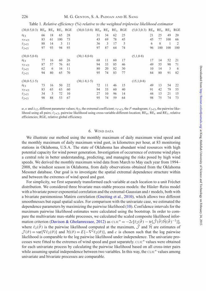
The estimation methods provide essentially unbiased estimators for the configuration ofparameters that we considered. Results are reported in the Supplementary Material. Table 1 showsthat some methods are more efficient than others.
The F-madogram estimator performed better than the extremal-coefficient estimator in almostall parameter settings. Overall, these two empirical estimators performed better than the pairwiselikelihood estimator using only cross-variable-different-location pairs. The pairwise likelihoodestimators that use all pairs outperform the empirical estimators. Although the pairwise likeli-hood based only on crossed pairs provides fairly quick estimates, a considerable loss of informa-tion is to be expected. In almost all cases, the relative global efficiency of the pairwise likelihoodbased on all the pairs, relative to triplewise weighted likelihood, is less than 100%, with thesmallest value being 64%. The same is true for the relative global efficiencies. This indicates anefficiency gain from using our proposed likelihood over all the other methods. In addition, thebenefit of using the weighted triplewise likelihood is more pronounced when the spatial depen-dence range is at a larger scale or when the cross-dependence is weak. Finally, we also noticethat the efficiency gain of using the weighted triplewise likelihood is not always more substantialfor smoother spatial fields, as found in Genton et al. (2011) and Huser & Davison (2013). Thissuggests that in the multivariate case, our proposed composite likelihood can be beneficial fromthe point of view of statistical and computational efficiency.
A second simulation study was performed considering a trivariate Husler–Reiss max-stableprocess. The results corroborate the findings above and are reported in the SupplementaryMaterial.
at King A
bdullah University of Science and T
echnology on February 24, 2015http://biom
et.oxfordjournals.org/D
ownloaded from
226 M. G. GENTON, S. A. PADOAN AND H. SANG
Table 1. Relative efficiency (%) relative to the weighted triplewise likelihood estimator
(30,0·5,0·3) REα REκ REλ RGE
θCI 66 18 65 28νF-CI 83 61 100 73�2-CI 88 14 3 11�2-CI 97 93 94 93
(30,0·5,0·8)θCI 77 16 60 26νF-CI 87 57 76 61�2-CI 62 6 16 11�2-CI 94 80 65 70
(30,0·5,1·5)θCI 73 16 50 22νF-CI 83 65 63 60�2-CI 34 3 72 10�2-CI 98 88 53 67
(30,0·3,0·8) REα REκ REλ RGE
31 34 62 2543 69 78 4536 3 17 597 87 64 74
(30,1·8,0·8)68 11 60 1794 33 85 4680 20 82 3095 74 83 77
(30,1·8,1·5)72 11 46 1594 33 60 4027 10 96 1495 74 59 64
(5,0·3,0·3) REα REκ REλ RGE
21 25 49 2045 77 100 666 8 1 296 100 100 100
(5,1,0·8)17 14 52 2149 55 90 7110 14 3 684 80 91 82
(15,1,0·8)49 13 54 2291 42 79 5544 13 21 1598 75 74 73
α, κ and λ12, different parameter values; θCI, the extremal coefficient; νF-CI, the F-madogram; �2-CI, the pairwise like-lihood using all pairs; �2-CI, pairwise likelihood using cross-variable-different-location; REα , REκ and REλ, relativeefficiencies; RGE, relative global efficiency.
6. WIND DATA
We illustrate our method using the monthly maximum of daily maximum wind speed andthe monthly maximum of daily maximum wind gust, in kilometres per hour, at 83 monitoringstations in Oklahoma, U.S.A. The state of Oklahoma has abundant wind resources with highpotential capacity for wind power generation. Investigation of occurrence of extreme wind playsa central role in better understanding, predicting, and managing the risks posed by high windspeeds. We derived the monthly maximum wind data from March to May each year from 1994–2008, the windiest season in Oklahoma, from daily observations obtained from the OklahomaMesonet database. Our goal is to investigate the spatial extremal dependence structure withinand between the extremes of wind speed and gust.
For simplicity, we first separately transformed each variable at each location to a unit Frechetdistribution. We considered three bivariate max-stable process models: the Husler–Reiss modelwith a bivariate power exponential correlation and the extremal-Gaussian and t models, both witha bivariate parsimonious Matern correlation (Gneiting et al., 2010), which allows two differentsmoothnesses but equal spatial scales. For comparison with the univariate case, we estimated thedependence parameters by maximizing the pairwise likelihood (10). Confidence intervals for themaximum pairwise likelihood estimates were calculated using the bootstrap. In order to com-pare the multivariate max-stable processes, we calculated the scaled composite likelihood infor-mation criterion (Davison & Gholamrezaee, 2012) as CLIC∗ = −2c[�2(ϑ)− tr{J (ϑ)H(ϑ)−1}],where �2(ϑ) is the pairwise likelihood computed at the maximum, J and H are estimates ofJ (ϑ)= var{∇�2(ϑ)} and H(ϑ)= E{−∇2�2(ϑ)}, and c is chosen such that the log pairwiselikelihood is comparable to the log pairwise likelihood under independence. The univariate pro-cesses were fitted to the extremes of wind speed and gust separately. CLIC∗ values were obtainedfor each univariate process by calculating the pairwise likelihood based on all cross-inter pairswhile assuming spatial independence between two variables. In this way, the CLIC∗ values amongunivariate and bivariate processes are comparable.
at King A
bdullah University of Science and T
echnology on February 24, 2015http://biom
et.oxfordjournals.org/D
ownloaded from

Multivariate max-stable spatial processes 227
Table 2. Estimates of the extremal dependence parameters, their 95% bootstrap confidenceintervals and CLIC
∗ scores under each max-stable process
Univariate random fieldsParameters α κ ν CLIC
∗
ModelsHusler–Reiss WS 1·7 (0·5,6·3) 0·44 (0·35,0·62) 70712– WG 2·6 (1·5,5·9) 0·50 (0·40,0·66) –Extremal-Gaussian WS 28 (29,49) 0·49 (0·27,0·55) 63170– WG 39 (26,47) 0·41 (0·43,0·72) –Extremal-t WS 119 (99,214) 0·31 (0·22,0·41) 1·75 (1·48,2·68) 63092– WG 108 (100,155) 0·34 (0·26,0·43) 2·09 (1·43,2·96) –
Bivariate random fieldsParameters α κ λ12/ρ12 ν CLIC
∗
ModelsHusler–Reiss 2·8 (0·9,7·6) 0·49 (0·38,0·66) 0·95 (0·87,1·04) 64791Extremal-Gaussian WS 29 (15,53) 0·58 (0·41,0·83) 0·76 (0·73,0·78) 62345– WG – 0·46 (0·27,0·73) – –Extremal-t WS 114 (100,172) 0·38 (0·29,0·50) 0·87 (0·84,0·90) 1·98 (1·53,2·82) 62251– WG – 0·30 (0·21,0·45) – – –
The scale parameter, α, is expressed in kilometres. In the univariate case, estimates concerning monthly maxima ofwind speed, WS, and wind gust, WG, are reported for each model. In the bivariate case, estimates of κ relate to windspeed and gust maxima, for the extremal-Gaussian and t processes. λ12 and ρ12 are the cross-component dependenceparameters for the bivariate Husler–Reiss and extremal-t processes. ν is the degrees of freedom of the extremal-tprocess.
Table 2 reports the estimation results. The results from the univariate models indicate that therange and the smoothness parameters are not significantly different between the wind speed andgust fields. This supports the use of a power exponential correlation with a constant range andsmoothness in the bivariate Husler–Reiss random field, and a parsimonious bivariate Matern witha constant range in the bivariate extremal-Gaussian and extremal-t fields.
The estimated cross-correlations from the bivariate processes indicate strong correlationbetween wind speed and gust. The estimated smoothness parameter from the bivariate extremal-t models is slightly smaller than those from the Husler–Reiss and bivariate extremal-Gaussianmodels, and the smoothness of the wind gust field is similar to that of the wind speed. Over-all, the smoothness parameters of the bivariate process are small, suggesting rough randomfields. According to CLIC
∗, all three multivariate models fit the data better than their univariatecounterparts. The bivariate extremal-t model has the smallest CLIC∗ among all three multivariatemodels, followed by the bivariate extremal-Gaussian model, suggesting that a multivariate corre-lation model that allows for different smoothnesses is preferred to one with a single smoothnessparameter. The extremal practical ranges (Davison et al., 2012) were calculated from the bivari-ate extremal-t model. Wind speed has practical ranges (6·9, 107) km, which are longer than (3·5,88) km, the practical ranges of wind gust. The extremal cross-component coefficient, θ [2]
i j , has
an estimated lower bound of 1·32. The estimate of θ [2]i j reaches 1·7 beyond 274 kilometres.
Figure 4 plots the binned and unbinned empirical estimates of extremal coefficients againstdistance, obtained with the F-madogram and the fitted extremal coefficient functions, obtainedwith a pairwise-likelihood estimator under each bivariate random field.
The fitted inter- and cross-component extremal coefficient functions, obtained with theextremal-t random field, match the binned empirical estimates well. The estimates obtained withthe bivariate Husler–Reiss random field appear to underestimate the extremal dependence to
at King A
bdullah University of Science and T
echnology on February 24, 2015http://biom
et.oxfordjournals.org/D
ownloaded from

228 M. G. GENTON, S. A. PADOAN AND H. SANG
0 100 200 300 400 500
1·0
1·2
1·4
1·6
1·8
2·0
2·2
0 100 200 300 400 500
1·0
1·2
1·4
1·6
1·8
2·0
2·2
0 100 200 300 400 500
1·0
1·2
1·4
1·6
1·8
2·0
2·2
qij[2] (h)
qi[2] (h) qj
[2] (h)
Distance (km)0 100 200 300 400 500
1·0
1·5
2·0
2·5
3·0
3·5
4·0
qij[4] (h)
Distance (km)
Fig. 4. Plots of the estimated inter- and cross-component extremal coefficient functionsversus distance. The grey circles are the pairwise empirical extremal coefficients and theblack circles are the binned empirical estimates. The vertical lines are the 95% confi-dence intervals. The curves are fitted extremal coefficient functions using the pairwiselikelihood under the bivariate Husler–Reiss (solid line), extremal-Gaussian (dashed line)
and extremal-t (dot-dashed line) random fields.
some extent, perhaps, partly due to the constraint of using a bivariate power correlation func-tion with a constant range and smoothness. Conversely, the estimates obtained with the bivariateextremal-Gaussian random field appear to overestimate the extremal dependence, because theextremal coefficient function under this model cannot exceed the upper bound, which is approx-imately 1·71 (Schlather, 2002).
Figure 5 shows 25-year return levels for wind speed and gust. The location and scale marginalparameters at unobserved locations were estimated using quadratic regressions on longitude andlatitude. The shape parameter was taken as constant. We sampled 10 000 realizations from aresidual bivariate extremal-t random field with unit Frechet marginals and with the dependencestructure reported in Table 2. We used the realizations of the residual random fields together withthe marginal parameters to transform the data back to generalized extreme-value marginals. Thereturn levels were then estimated using the empirical quantiles of the sampled random fields.Figure 5 maps the 25-year conditional return levels of wind speed/gust given wind gust/speed atthe same location or in Oklahoma City. The T -year conditional return level of wind speed/gustgiven wind gust/speed is defined as a threshold such that the conditional probability that windspeed/gust exceeds this threshold is 1/T , given that, at the same location, wind gust/speedexceeds its own T -year return level. The T -year conditional return level of wind speed/gustgiven the wind gust/speed in Oklahoma City is defined as a threshold such that the conditionalprobability that wind speed/gust exceeds this threshold is 1/T , given that the wind gust/speedin Oklahoma City exceeds its own T -year return level. The 25-year conditional return levels of
at King A
bdullah University of Science and T
echnology on February 24, 2015http://biom
et.oxfordjournals.org/D
ownloaded from
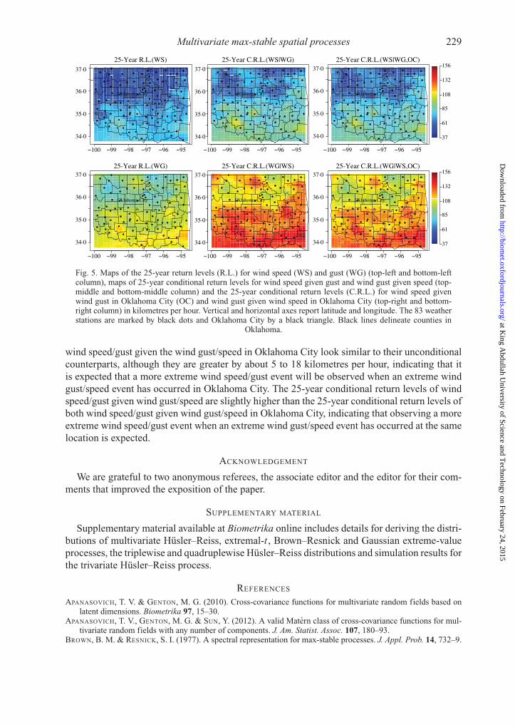
Multivariate max-stable spatial processes 229
37
61
85
108
132
156
37
61
85
108
132
156
−100 −99 −98 −97 −96 −95 −100 −99 −98 −97 −95 −100 −99 −98 −97 −96 −95−96
−100 −99 −98 −97 −96 −95 −100 −99 −98 −97 −95 −100 −99 −98 −97 −96 −95−96
25-Year R.L.(WS)
Oklahoma City
25-Year C.R.L.(WS|WG)
Oklahoma City
25-Year C.R.L.(WS|WG,OC)
Oklahoma City
34·0
35·0
36·0
37·0
34·0
35·0
36·0
37·0
34·0
35·0
36·0
37·0
34·0
35·0
36·0
37·0
34·0
35·0
36·0
37·0
34·0
35·0
36·0
37·025-Year R.L.(WG)
Oklahoma City
25-Year C.R.L.(WG|WS)
Oklahoma City
25-Year C.R.L.(WG|WS,OC)
Oklahoma City
Fig. 5. Maps of the 25-year return levels (R.L.) for wind speed (WS) and gust (WG) (top-left and bottom-leftcolumn), maps of 25-year conditional return levels for wind speed given gust and wind gust given speed (top-middle and bottom-middle column) and the 25-year conditional return levels (C.R.L.) for wind speed givenwind gust in Oklahoma City (OC) and wind gust given wind speed in Oklahoma City (top-right and bottom-right column) in kilometres per hour. Vertical and horizontal axes report latitude and longitude. The 83 weatherstations are marked by black dots and Oklahoma City by a black triangle. Black lines delineate counties in
Oklahoma.
wind speed/gust given the wind gust/speed in Oklahoma City look similar to their unconditionalcounterparts, although they are greater by about 5 to 18 kilometres per hour, indicating that itis expected that a more extreme wind speed/gust event will be observed when an extreme windgust/speed event has occurred in Oklahoma City. The 25-year conditional return levels of windspeed/gust given wind gust/speed are slightly higher than the 25-year conditional return levels ofboth wind speed/gust given wind gust/speed in Oklahoma City, indicating that observing a moreextreme wind speed/gust event when an extreme wind gust/speed event has occurred at the samelocation is expected.
ACKNOWLEDGEMENT
We are grateful to two anonymous referees, the associate editor and the editor for their com-ments that improved the exposition of the paper.
SUPPLEMENTARY MATERIAL
Supplementary material available at Biometrika online includes details for deriving the distri-butions of multivariate Husler–Reiss, extremal-t , Brown–Resnick and Gaussian extreme-valueprocesses, the triplewise and quadruplewise Husler–Reiss distributions and simulation results forthe trivariate Husler–Reiss process.
REFERENCES
APANASOVICH, T. V. & GENTON, M. G. (2010). Cross-covariance functions for multivariate random fields based onlatent dimensions. Biometrika 97, 15–30.
APANASOVICH, T. V., GENTON, M. G. & SUN, Y. (2012). A valid Matern class of cross-covariance functions for mul-tivariate random fields with any number of components. J. Am. Statist. Assoc. 107, 180–93.
BROWN, B. M. & RESNICK, S. I. (1977). A spectral representation for max-stable processes. J. Appl. Prob. 14, 732–9.
at King A
bdullah University of Science and T
echnology on February 24, 2015http://biom
et.oxfordjournals.org/D
ownloaded from
230 M. G. GENTON, S. A. PADOAN AND H. SANG
COOLEY, D., NAVEAU, P. & PONCET, P. (2006). Variograms for spatial max-stable random fields. In Dependence inProbability and Statistics, Ed. P. Bickel, P. Diggle, S. Fienberg, U. Gather, I. Olkin, S. Zeger, P. Bertail, P. Soulierand P. Doukhan, Lecture Notes in Statistics 187. Springer, pp. 373–90.
COOLEY, D., CISEWSKI, J., ERHARDT, R. J., JEON, S., MANNSHARDT, E., OMOLO B. O. & SUN, Y. (2012). A survey ofspatial extremes: Measuring spatial dependence and modeling spatial effects. REVSTAT Statist. J. 10, 135–65.
DAVIS, R. A., KLUPPERLBERG, C. & STEINKOHL, C. (2013). Statistical inference for max-stable processes in spaceand time. J. R. Statist. Soc. B 75, 791–819.
DAVISON, A. C. & GHOLAMREZAEE, M. (2012). Geostatistics of extremes. Proc. R. Soc. A 468, 581–608.DAVISON, A. C. & HUSER, R. (2015). Statistics of extremes. Ann. Rev. Statist. Appl. 2, in press.DAVISON, A. C., PADOAN, S. A. & RIBATET, M. (2012). Statistical modeling of spatial extremes. Statist. Sci. 27,
161–86.DE HAAN, L. (1984). A spectral representation for max-stable processes. Ann. Prob. 12, 1194–204.DE HAAN, L. & FERREIRA, A. (2006). Extreme Value Theory: An Introduction. New York: Springer.DE HAAN, L. & ZHOU, C. (2011). Extreme residual dependence for random vectors and processes. Adv. Appl. Prob.
43, 217–42.GENTON, M. G. & KLEIBER, W. (2015). Cross-covariance functions for multivariate geostatistics (with discussion).
Statist. Sci., in press.GENTON, M. G., MA, Y. & SANG, H. (2011). On the likelihood function of Gaussian max-stable processes. Biometrika
98, 481–8.GNEITING, T., KLEIBER, W. & SCHLATHER, M. (2010). Matern cross-covariance functions for multivariate random
fields. J. Am. Statist. Assoc. 105, 1167–77.HUSER, R. & DAVISON, A. C. (2013). Composite likelihood estimation for the Brown–Resnick process. Biometrika
100, 511–8.HUSER, R. & DAVISON, A. C. (2014). Space-time modelling of extreme events. J. R. Statist. Soc. B 76, 439–61.HUSLER, J. & REISS, R.-D. (1989). Maxima of normal random vectors: Between independence and complete depen-
dence. Statist. Prob. Lett. 7, 283–6.KABLUCHKO, Z. L. (2009). Extremes of space-time Gaussian processes. Stoch. Proces. Appl. 119, 3962–80.KABLUCHKO, Z. L. (2011). Extremes of independent Gaussian processes. Extremes 14, 285–310.KABLUCHKO, Z., SCHLATHER, M. & DE HAAN, L. (2009). Stationary max-stable fields associated to negative definite
functions. Ann. Prob. 37, 2042–65.KLEIBER, W. & GENTON, M. G. (2013). Spatially varying cross-correlation coefficients in the presence of nugget
effects. Biometrika 100, 213–20.LI, B. & ZHANG, H. (2011). An approach to modeling asymmetric multivariate spatial covariance structures. J. Mult.
Anal. 102, 1445–53.NIKOLOULOPOULOS, A. K., JOE, H. & LI, H. (2009). Extreme value properties of multivariate t copulas. Extremes 12,
129–48.OPITZ, T. (2013). Extremal t processes: Elliptical domain of attraction and a spectral representation. J. Mult. Anal.
122, 409–13.PADOAN, S. A., RIBATET, M. & SISSON, S. A. (2010). Likelihood-based inference for max-stable processes. J. Am.
Statist. Assoc. 105, 263–77.PADOAN, S. A. (2013a). Extreme dependence models based on event magnitude. J. Mult. Anal. 122, 1–19.PADOAN, S. A. (2013b). Max-Stable Processes. Encyclopedia of Environmetrics 4, John Wiley & Sons, doi:
10.1002/9780470057339.vnn022.RESNICK, S. I. (1987). Extreme Values, Point Processes and Regular Variation, 1st ed. New York: Springer Verlag.RIBATET, M., COOLEY, D. & DAVISON, A. C. (2012). Bayesian inference from composite likelihoods, with an applica-
tion to spatial extremes. Statist. Sinica 22, 813–45.RIBATET, M. (2013). Spatial extremes: Max-stable processes at work. J. Soc. Francaise Statist. 154, 156–77.RØISLIEN, J. & OMRE, H. (2006). T-distributed random fields: A parametric model for heavy-tailed well-log data.
Math. Geol. 38, 821–49.SANG, H. & GENTON, M. G. (2014). Tapered composite likelihood for spatial max-stable models. Spat. Statist. 8,
86–103.SCHLATHER, M. (2002). Models for stationary max-stable random fields. Extremes 5, 33–44.SCHLATHER, M. & TAWN, J. A. (2003). A dependence measure for multivariate and spatial extreme values: Properties
and inference. Biometrika 90, 139–54.VARIN, C., REID, N. & FIRTH, D. (2011). An overview of composite likelihood methods. Statist. Sinica 21, 5–42.WADSWORTH, J. L. & TAWN, J. A. (2012). Dependence modelling for spatial extremes. Biometrika 99, 253–72.WADSWORTH, J. L. & TAWN, J. A. (2014). Efficient inference for spatial extreme value processes associated to log-
Gaussian random functions. Biometrika 101, 1–15.ZHANG, Z. & SMITH, R. L. (2004). The behavior of multivariate maxima of moving maxima processes. J. Appl. Prob.
41, 1113–23.
[Received April 2013. Revised October 2014]
at King A
bdullah University of Science and T
echnology on February 24, 2015http://biom
et.oxfordjournals.org/D
ownloaded from