Multivariate dependence between stock and commodity marketsA preliminary draft

Manel Soury, Phd candidate

Aix-Marseille University, (AMSE), 2 rue de la Charite, 13002 Marseille, France

Abstract

I investigate the multivariate dependence between price returns for commodities from different sectors

(energy, agriculture, precious metals and industrial metals ) with some major equities (SP500, FTSE10,

DAX30, CAC40, MSCI China and MSCI India). The sample runs from January 1993 to February 2016

and I explore different sub-samples more in details. For that I use the Regular Vine Copula model as it is

more flexible than GARCH-type models in the modelling of complex dependency patterns by arranging

a tree structure to explore multiple correlations between the variables. The empirical results suggest that

the dependencies fluctuate and change each time depending on the period considered. And this is not

just related to the financial crisis but also to the effect of the ’financialization’ of commodity markets. In

addition, there is a low co-movements across equities and commodities in particular for precious metals

and agriculture sectors which confirm their position as a safe-haven. The link between the stock market

and industrial metals and energy related commodities is stronger than with the remaining two sectors,

specially for industrial metals in the chinese case, and it remains high even after the crisis. For further

details, I use the Vector Error Correction model to study their long-run and short-run causality. The

efficiency of the Vine copula model have been tested using a risk management analysis based on the Value

at Risk (VaR) measure and it seems to outperform the other classical method considered (covariance-

variance).

Key words: Commodities, equities, volatility, correlations, Regular Vine copula

JEL:C15, C46, G15.

1. Introduction

Usually, raw materials and more generally commodities’ production is linked to a specific geographical

areas. However, their consumption concerns all countries from all continents, that’s why, it is more linked

to global international markets. Consequently, their prices and their volatilities play an important role in

global economic activity and growth. However, contrarily to other financial assets as equities and bonds,

that can also be influenced by other external factors like speculations, wars, crisis, economic activity

. . . , commodities prices are mainly affected by fundamentals of the economy: the supply and demand

variations specially since demand is ’generally’ strongly inelastic . Meaning, an increase in demand of a

certain ressources will generate higher prices for the corresponding good, and so investements related to

Email addresses: manel.soury@yahoo.fr ( Manel Soury, Phd candidate ), manel.soury@yahoo.fr ( Manel Soury,Phd candidate )

Preprint submitted to Journal of LATEX Templates February 7, 2017

this commodity will further increase resulting on higher production, causing an excess in supply and a

decrease of the prices compared to before and thus a drop in production. This cyclical pattern is usually

followed by commodities. Because of this difference of behaviour between the price of commodities and

traditional financial assets, their correlations tend to be low or even negative. Many researchers have

pointed out this fact: Erb and Harvey (2006), Gorton and Geert (2006), Byksahin et al (2010) and Chong

and Miffre (2010).

This lack of comovements between commodities and financial markets represented an attractive feature

for investors and financial actors with various types of investement funds. They were more eager and less

reluctant to add commodity futures in their portfolios for diversification purpose. And so, commodities

become more and more a popular asset in financial and derivative markets and were included in the

portfolio allocation process by financial institutions and investors for speculation and trading just like eq-

uities and bonds. This has implied a strong increase of commodities transactions for both diversification

purposes to minimize the risk of investements and for speculation purposes as well. Treating commodi-

ties like other financial assets made them behave more like ones, therefore, correlation between the two

class is no longer inexistant and their dependency increased considerably. This phenomenon is referred

to as the financialization of commodity market1. Although it was initiated around early 2000s, when

the finanancial and commodity markets become more integrated, its direct effect on commodities was

magnified on the period of the global crisis and the nature of their fluctuations has changed considerably.

This is in line with some researches in the litterature that pointed out this phenomenon as in Tang and

Xiong (2012), Cheng and Xiong (2014), Basak and Pavlova (2016).

Naturally, the volatilities of this particulur class of assets was affected by these changes specially

during the recent years (beginning 2000’s). As commodity prices continued to increase and to oscillate

between low and high due to supply and demand variations as well as the financialization of commodities,

their prices become more volatile than ever. Figure 1 shows the brute series and their returns of the SP500

stock market and the SP GSCI commodity index, one of the most representative commodity index of the

global economy. One can see that both SP500 and SP GSCI prices fell down around 2007-2008, and it

seems their dependency have particularily strengthened since then. This relationship however exsisted

long time before the crisis as commodity and financial markets were more integrated in the last decade

and we can see the changes in the prices of the SP GSCI around early 2000’s: There is a little (gentle)

rise at the beginning of the period with an acceleration in the price increase after 2005. Of course, the

same goes for their volatilities, it had ups and down and was accentuated during the financial crisis for

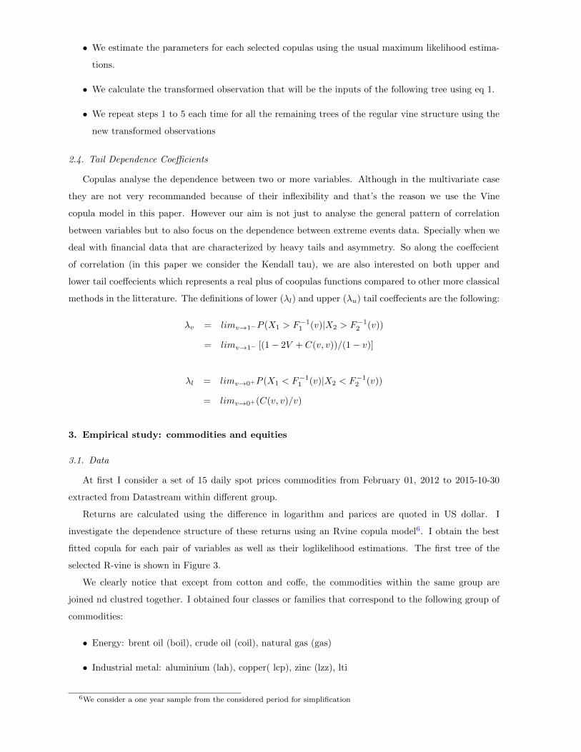
both series. Figure 2 represents the prices of different commodity indices for different sectors (agriculture,

energy, precious metal, industrial metal, livestock)2 and their corresponding returns. Overall, they also

1 total ammount of different commodity instruments purchased by financial institutions and investors increased from 15

to 200 billion between 2003 and mid-2008, source: US Commodity Futures Trading Commission.2The SP GSCI Agriculture Index shows a global idea about the agriculture sector in commodity asset in general. It is

composed of 8 different agriculture commodities (wheat, Kansas wheat, corn, sugar, soybean, coffee, cocoa and cotton)The

SP GSCI energy index represents a benshmark of the energy sector in the commodity class. It includes six commodities:

WTI light sweeT crude oil, Brent crude oil, Gas oil, Heating oil, RBOB gasoline and natural gas. The SP GSCI precious

2

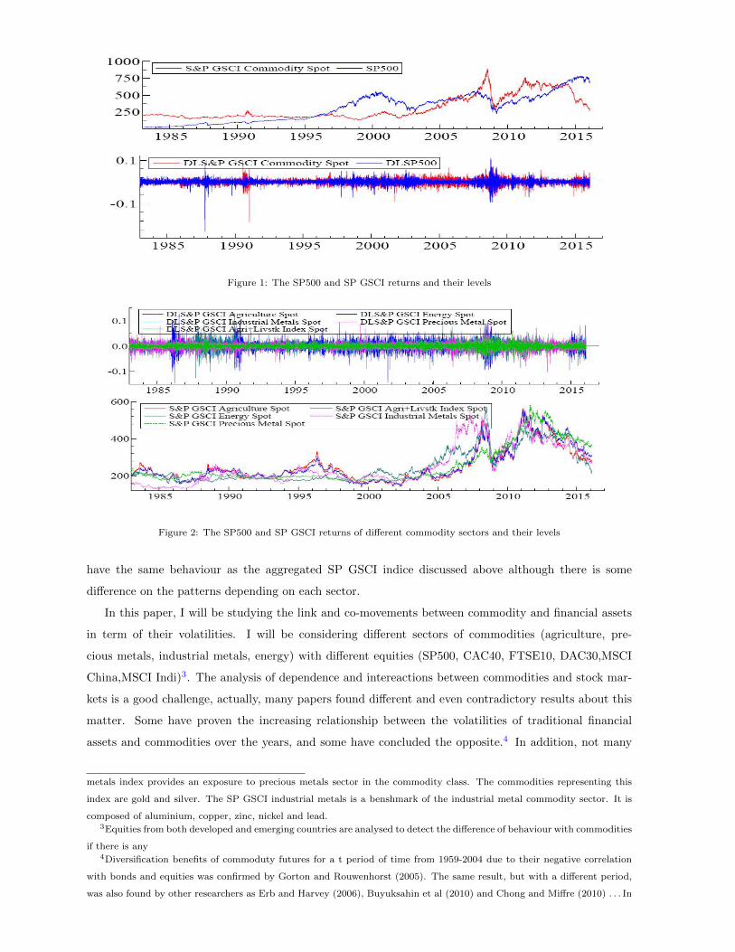
Figure 1: The SP500 and SP GSCI returns and their levels

Figure 2: The SP500 and SP GSCI returns of different commodity sectors and their levels

have the same behaviour as the aggregated SP GSCI indice discussed above although there is some

difference on the patterns depending on each sector.

In this paper, I will be studying the link and co-movements between commodity and financial assets

in term of their volatilities. I will be considering different sectors of commodities (agriculture, pre-

cious metals, industrial metals, energy) with different equities (SP500, CAC40, FTSE10, DAC30,MSCI

China,MSCI Indi)3. The analysis of dependence and intereactions between commodities and stock mar-

kets is a good challenge, actually, many papers found different and even contradictory results about this

matter. Some have proven the increasing relationship between the volatilities of traditional financial

assets and commodities over the years, and some have concluded the opposite.4 In addition, not many

metals index provides an exposure to precious metals sector in the commodity class. The commodities representing this

index are gold and silver. The SP GSCI industrial metals is a benshmark of the industrial metal commodity sector. It is

composed of aluminium, copper, zinc, nickel and lead.3Equities from both developed and emerging countries are analysed to detect the difference of behaviour with commodities

if there is any4Diversification benefits of commoduty futures for a t period of time from 1959-2004 due to their negative correlation

with bonds and equities was confirmed by Gorton and Rouwenhorst (2005). The same result, but with a different period,

was also found by other researchers as Erb and Harvey (2006), Buyuksahin et al (2010) and Chong and Miffre (2010) . . . In

3

researchers have studied this relationship between the two markets in the global economy. Usually they

focus only on a certain commodity or a sector: Hammoudeh and Li (2008), Arouri et al (2012), Ma-

rimoutou and Soury (2015). . . treated only the energy sector. They consider only a specific country or

region: Yamori (2011) for Japan, Roache (2012) for China, Boako and Alagidede (2016) for Africa . . . Or

they consider the series in level not in terms of their volatilities. Also this is the first paper to investigate

dependecy in the multivariate case and not just the biavariate one. Among the researchers who have

studied the dynamics of the prices of stock markets and commodities there is: Choi and Hammoudeh

(2010), using the DCC model, showed that correlations among commodities like oil, copper, gold and

silver were in the rise since 2003 but was decreased between them and the SP500. Creti et al (2013)

investigated dependence between commodities from agriculture, industrial metal and energy markets and

major equity indices ( SP500,DAX30,CAC40 and FTSE100) using static annd dynamic copulas based on

Patton (2006). They found that their dependence commodity is dynamic and symmetric and increased

considerably starting from 2003 reaching its peak at 2008. Silvennoinen and Thorp (2013) showed that

investors could take advantage from the interdependence of commodity and stock markets by diversifying

their portfolios. Charlot et al (2016) studied the co-movement across commodities and between them

and traditional returns using the Regime Switching Dynamic Correlation model. They found that their

correlations increased particularily during the global financial crisis although the influence of the finan-

cialization phenomenon started from mid-2005. And that it reverted to the pre-crisis level from April

2013.

Many reviews of the litterature have analysed and modeled volatilities of the returns and their de-

pendency . Engle (2002) introduced the DCC (Dynamic Conditional Correlation) model, which is more

flexible compared to the GARCH family to model dynamic correlation.More recently, the Generalized

Autoregressive Score (GAS) models (Creal et al (2008)), also known as the Dynamic Conditional Score

(DCS) model, an observation driven model which specify time varying parameters as volatilities or cor-

relation represents a good choice for 2-dimensional data. There is another approach, copula functions for

analysing time varying dependency between the returns. It have been intensively used these recent years

because it offers many advantages compared to traditional regression tools. It does not assume elliptical

distributions of the data and can be used even when the hypopthesis of normality is rejected. In addition,

it takes into account the stylised facts characterising financial time series( excess kurtosis, asymmetry,

non linearity . . . ). Patton (2006a) was the one who pioneered this method and made it more flexible

to take into account the change and the structure of dependency over time between the returns. This

approach can be applied even when the hypopthesis of normality is rejected and whene correlations are

subject to asymmetry and non linearity. There is an abundant litterature dealing with copula function

(Jondeau and Rockinger (2006), Embrechets et al (2010), Remillard et al(2009), Marimoutou and Soury

(2015) . . . ) among many others.

Instead of focusing only on the bivariate case, which have been treated by some rearchers, I choose

to model the multivariate co-movements between commodities and stock returns by considering many

contrast, Tang and Xiong (2010), Silvennoinen and Thor (2010) and Byksahin and Robe (2011) . . . reached the opposite

conclusion, commodity and financial assets markets are integrated.

4

sectors of commodities and many equities. A flexible approach to model multivariate distributions in

high d-dimenesional data is the Vine copulas, also called the pair copula construction (PCC). Combined

with bivariate copulas, regular vines have proven to be a flexible tool for high-dimensional distributions.

As its name indicates, it decomposes a multivariate distribution function to a cascade or blocks of bi-

variate copulas between each pair of the studied variables ’pair-copula’. In other words, it is a flexible

graphical model which allows to construct a multivariate distribution by building a product of d(d−1)/2

bivariate copulas. Pair copula construction was first introduced by Joe (1996) followed after by Bedford

and Cooke (2001, 2002). Bedford and Cooke (2002) developed the theory of Vines to help organize the

different structures obtained by the PCC model. The most known and used structures are the regular

Vine (R-vine), the canonical vine (C-vine), and the D-vine. Then, Czado et al (2009) studied it with

more depth, focusing on the estimations, inferences, and applications of this relatively new method.

Vina copula model is also an effecient method to use for risk management by investors and financial

institutions to calculate with more precision the risk of their investements. Usually, their portfolios are

constructed from a large number of assets and not just two. So the Vine copula as it is more flexible in

modeling multivariate distributions can clearly outperform other classical approach. I employ the Vine

copula model versus the multivariate normal distribution to analyse the Value-at-Risk of a portfolio and

I found that the latter one tend to underestimate the risk compared to the Vine approach.

Some backround and theory about copulas functions and the particular case of Vines are presented in the

next section, followed by the empirical study about commodities and stock markets before concluding.

2. Methodology

In this section I will introduce briefly some basic theory and notions about copulas, Vine structure

and their different measures of dependence. For more details about the Vine Copulais methedology please

refer to the Appendix.

2.1. Copula

An n-dimensional copula C(F (u1), . . . , F (un))5 is a cumulative distribution function with uniform

marginals F (u1), . . . , F (un). Based on Skalr (1959), if the variables (u1, . . . un) are continuous with the

corresponding cumulative distribution fucntions F (u1), . . . , F (un) then the copula C(F (u1), . . . , F (un))

represents the n-variate cumulative distribution function of (u1, . . . un). And we can write the following:

F ((u1), . . . , F (un)) = C(F (u1), . . . , F (un)) (1)

And if F (u1), . . . , F (un) are also continuous then the copula F ((u1), . . . , F (un) = exists and is unique.

The above Equation represents the decomposition of the joint distribution function into marginal dis-

tributions that describe the individual behaviour of each variables and the copula C that captures the

dependence structure between them.

5(see Nelsen (2007) for more detail

5

2.2. Pair Copula Decomposition, PCD

The Pair Copula Decomposition approach was proposed by Joe (1996). Bedford and Cooke (2001,2002)

have extended it by considering the general case based on the graphical probabilistic model. The PCD

is defined as the following.

A density function f (u1, . . . , un)canbefactorizedas : f(u1, . . . , un) = f(un)f(un−1|u1)f(u1|u2, . . . , un).(2)

In the general case, the marginal densities ( the righthand of Eq (2)) can be expressed as:

f(ui|ν) = cuiνj |ν−j(F (ui|ν−j), F (νj |ν−j)).f(ui|ν−j) (3)

where ν = {ui+1, . . . xn} is the number of variables after ui, it is called the conditioning set of the density

of ui. νj is a set of variables belonging to ν and ν−j are the remaining variables also from ν but not

including variables from νj . In other words, νj ∪ν−j = ν. i = 1, . . . (n− 1) and c(, ) is the densitty copula

function. Thus, one can decompose the density of f(ui|ν) to the product of the marginal density function

of ui and a bivariate copula density function c. If we decompose in the same way all the marginal densities

in eq 2 then f(u1, . . . , un) will be written as a product of the marginal densities of the set of variables

u1, . . . , un and a bivariate density copulas. This is what we refer to as the pair-copula construction of

f(u1, . . . , un). Using the PCC approach, many expressions of the density function are obtained depending

on the selection of the set of variables in νj (and there are many possibilities). Two particular cases of

PCC, the CVINE and the DVINE densities are given below:

C-Vine

f(u1, . . . , un) =

n∏k=1

fk(uk)

n−1∏j=1

n−j∏i=1

cj,j+i|1,...,j−1.(Fj|1,...,j−1(uj |u1, . . . , uj−1), Fj+i|1,...,j−1(ui+j |u1,...,j−1))

D-Vine

f(u1, . . . , un) =n∏k=1

fk(uk)n−1∏j=1

n−j∏i=1

ci,i+j|i+1,...,i+j−1.(Fi|i+1,...,i+j−1(ui|ui+1,...,i+j−1), Fi+j|i+1,...,i+j−1(ui+j |ui+1,...,i+j−1))

Cvines and Dvines are two particular cases of a more general case of PCC decompositions:Rvines. Rvines

are a more global structure that encompasses CVINE, Dvine and more others. Rvine were introduced by

Bedford and Cooke (2002) to help organize the different structures given by PCC. Below are the main

points of this model. For more details about Rvines please refer to the work of Dissmann et al. (2013).

2.3. R-Vine Specification

To identifu and estimate the regular vine (RVine) structure, we refer to the sequential procedure,

based on Dissmann et al. (2013).

• We select the structure of the tree by the maximisation of the sum of the absolute empirical Kendall

tau coefficients by using the algorithm proposed by Prim (1957).

• We select the best fitted copula family for each pair of the tree (already selected in step 1) by

minimizing the AIC criteria.

6

• We estimate the parameters for each selected copulas using the usual maximum likelihood estima-

tions.

• We calculate the transformed observation that will be the inputs of the following tree using eq 1.

• We repeat steps 1 to 5 each time for all the remaining trees of the regular vine structure using the

new transformed observations

2.4. Tail Dependence Coefficients

Copulas analyse the dependence between two or more variables. Although in the multivariate case

they are not very recommanded because of their inflexibility and that’s the reason we use the Vine

copula model in this paper. However our aim is not just to analyse the general pattern of correlation

between variables but to also focus on the dependence between extreme events data. Specially when we

deal with financial data that are characterized by heavy tails and asymmetry. So along the coeffecient

of correlation (in this paper we consider the Kendall tau), we are also interested on both upper and

lower tail coeffecients which represents a real plus of coopulas functions compared to other more classical

methods in the litterature. The definitions of lower (λl) and upper (λu) tail coeffecients are the following:

λv = limv→1−P (X1 > F−11 (v)|X2 > F−12 (v))

= limv→1− [(1− 2V + C(v, v))/(1− v)]

λl = limv→0+P (X1 < F−11 (v)|X2 < F−12 (v))

= limv→0+(C(v, v)/v)

3. Empirical study: commodities and equities

3.1. Data

At first I consider a set of 15 daily spot prices commodities from February 01, 2012 to 2015-10-30

extracted from Datastream within different group.

Returns are calculated using the difference in logarithm and parices are quoted in US dollar. I

investigate the dependence structure of these returns using an Rvine copula model6. I obtain the best

fitted copula for each pair of variables as well as their loglikelihood estimations. The first tree of the

selected R-vine is shown in Figure 3.

We clearly notice that except from cotton and coffe, the commodities within the same group are

joined nd clustred together. I obtained four classes or families that correspond to the following group of

commodities:

• Energy: brent oil (boil), crude oil (coil), natural gas (gas)

• Industrial metal: aluminium (lah), copper( lcp), zinc (lzz), lti

6We consider a one year sample from the considered period for simplification

7

Figure 3: The first tree of the R-vine structure with 15 commodities, red circle for agriculture, blue for industrial metals,

yellow for precious metals and green for energy

• Agricultural: wheat (wheat), sugar (wsug), cotton (cott), soy (soy)

• Precious metals:gold (gold), silver (silv), platinum (plat), palladium (pall)

Based on this finding I may simplify the work by considering only one of the most popular commodity

aggregate indices, the SP GSCI Commodity, and its sub-indices (the SP GSCI Agriculture Spot, the SP

GSCI Energy Spot, the SP GSCI Industrial Metals Spot, the SP GSCI Precious Metal Spot) to account

for each group or sector of commodities.

By considering each given group of commodities given by the Rvine structure and substitute the set

of commodities by a more global indice for the same group I manage to reduce the number of variables

from 18 to only 4 while relatively having the same amount of information. For the stock market here

represented by the equities , I assess for six major equity indices: SP500, DAX30, FTSE10, CAC40,

MSCI China and MSCI India. I analyse the evolution of their correlations over time with the SP GSCI

Commodity using the Gaussian copula (figure 4).7

I notice that the dependence patterns are almost the same for the SP500, DAX30, FTSE10 and

CAC40 equities and one may say that the results are quite robust to the choice of equity price. However

correlations with the commodity index SP GSCI with both the chineese and the indian equities differ

very much from the others. Hence, in the remaining of this papaer, I choose to work with the SP500 as

7I only show the conditional correlation given by the Gaussian copula given that it corresponds to the benshmark copula

and since in our case and at this point we only wish to have the general aspect of the correlation and their patterns ,without

entering into the details like tail dependencies, to see if they differ with the choice of equity.

8

a representative for DAX30, FTSE10 and CAC40 which is relatively expected. The SP500 is the most

global and used equity in global economy. But I will also consider both the chinese and indian equities

since they both showed very different dependency patterns with the commodity market.

CACSPG FTSESPG

DAXSPG SPSPG

1990 1995 2000 2005 2010 2015

0.0

0.5CACSPG FTSESPG

DAXSPG SPSPG

INDSPG SPSPG

1990 1995 2000 2005 2010 2015

0.00

0.25

INDSPG SPSPG

SPSPG CHINSPG

1990 1995 2000 2005 2010 2015

0.0

0.5 SPSPG CHINSPG

Figure 4: The time varying correlations of different equities with the SP GSCI commodity index

To summarize, I will be working with for commodity indices that account for energy, industrial,

precious metals and industrial metals and three equities (SP500, MSCI China and MSCI I ndia) that

represent the stock market. Daily data is chosen for all variables with a total of 6022 trading days

covering the period from 01/01/1993 to 01/02/2016. Table 1 presents the usual summary statistics. All

Agri Eng Indus Prec SP China India

Mean 6.1932e-005 8.1656e-005 8.0671e-005 0.00021072 0.00024799 -0.00010963 0.00024153

SD 0.011685 0.01877 0.013094 0.010894 0.011487 0.019079 0.016773

Skewness -0.074067 -0.18503 -0.23022 -0.28343 -0.24863 0.051124 -0.075533

Excess Kurtosis 2.9594 2.8213 3.5960 7.1842 8.9514 5.7648 6.7641

Jarque Bera 2202.6 2031.3 3297.2 13029. 20164 8341.4 11486

KPSS 0 0 0 0 0 0 0

Table 1: Summary statistics for the returns of the given variables, for the skewness, excess kurtosis, Jarque Bera test and

KPSS test, the significance level is 1% .

five indices recorded are stationary and do not present any unit root. The mean of the returns are small

and near zero, indicating that there is no significant trend in the data. They all exhibit negative skewness

and kurtosis in excess of 3, indicating possibility of fat tails and asymmetry in the data. The Jarque Bera

test suggests the non normality of the data.

9

3.2. Marginals models

Before analysing the dependence between the set of variables, the series have to be corrected from any

heteregoneity or noises due to the presence of time-varying volatility (ARCH) effects, autocorrelations or

sudden changes and outliers. To account for this problem, I fit an ARMA- (Garch, Egarch, Gas) model

with different error terms (Normal, student, skewed student). I choose the best suited model for each

index return based on its information criteria (Aic/Bic). Results of the estimation are presented in Table

2. The ARMA(1,1)-GARCH(1,1)-Normal was best fitted for the SP Gsci energy and industrial metals.

ARMA(1,0)-Garch-skewed student for the SP GSCI agricultural, ARMA(1,0)-GARCH-Student for the

SP500 and the SP GSCI precious metal index. ARMA(0,1)-GARCH-Student is assigned to the chineese

equity MSCI China, and the GARCH-Normal to the indian equith MSCI India.

α and β, the variance equation parameters are statistically significant at the 1% level and their sum

is close to 1 implying the presence of ARCH and GARCH effects on the returns and that the models

are stationary and their volatilities are highly persistent. The tail parameter is significant suggesting

that the skewed student distribution for the error terms works reasonably well for the returns of the SP

GSCI agricultural index. However there is no hint of asymmetry since its parameter is insignificant. In

addition by referring to the ARCH-LM and the Box Pierce tests to the resulting standardized innovations

, overall, all the models are well specified and there is no remaining autocorrelation and ARCH effects in

the residuals. Then the standardized residuals from each fitted model are transformed into uniform copula

input using the empirical cumulative distribution function. I then test for the adequacy of the inputs

copulas, by verefying whether they are drawn from the uniform distribution on [0,1]. For that, some

goodness-of-fit tests are performed: Anderson Darling (AD), Kolmogorov-Smirnov (KS), and Cramer-

von Mises. The results in table 3 indicate clearly that the null hypothesis that the empirical distribution

is consistent with the uniform distribution on [0,1] can be accepted. Thus the vine model can correctly

use the uniform copula data to capture dependence between the returns of the studied variables.

3.3. Vine model

After estimating the marginals with a GARCH model, I transform the extracted standard residuals

to uniform variables for copula inputs. Our aim is to investigate the dependence between the different

commodities and equities from 01/1993 to 01/2016.8To capture these co-movements, I employ the R-Vine

copulas model explained above in section 2. Estimation are given by the maximum likelihood method.

The mixed R-Vine9 model is compared with the C-vine model, a particular case of Rvine where there is a

root node in each tree, and the Gaussian Rvine10 model as a benshmark. All models are estimated using

the VineCopula R package (Schepsmeier et al. 2016). I use the information criteria as well as the Vuong

test to determine which model fits best the data. Table 4 and 5 show the results for the three alternative

models. Both the mixed Rvine and the Cvine are preferred over the the Gauss Rvine model by the

Vuong test in all three cases (with no correction or Akaike correction or Schwartz correction ). This test

8the data begins from the first available date given for the MSCI returns9the copulas families used for the pair-copulas are: Gaussian, Student, Clayton, Gumbel, Franck, Joe,BB (1,6,7,8), Tawn

with their rotated versions as well10I impose only the Gaussian copula between each pair of the variables and for all trees of the structure

10

agri eng indus prec sp china india

Mean equation

cst -0.00001 0 0 0 0 0 0.000

0.890 0.156 0.935 0.220 0 0.2492 0.0004

AR(1) 0.032 0.8104 0.429 0.500 -0.013 - -

0.002 0 0.182 0.044 0.158 - -

MA(1) - -0.812 -0.437 -0.546 - 0.113003 -

- 0 0.187 0.0227 - 0.0000 -

Variance equation

Cst(V) 0.008 0.023 0.006 0.008 0.008 0.036246 0.065247

0 0 0.006 0.001 0 0.0005 0.0000

ARCH(Alpha1) 0.052 0.061 0.039 0.042 0.065 0.08900 0.105745

0 0 0 0 0 0.00 0.0000

GARCH(Beta1) 0.941 0.933 0.956 0.958 0.928 0.9046 0.873435

0 0 0 0 0 0 0

Asymmetry 0.003 - - - - - -

0.77 - - - - - -

Tail 7.916 - - 3.690(stdDF)) - 5.394 STDf 5.8436 (tdf) -

0 - - 0 0 0 -

Gof

LL 27843.134 23042.927 25953.179 28207.974 28567.779 16470.2 16811.9

Q( 5) 0.11648 0.176 0.044 0 0.010 0.02035 0.00

Q(5)2 0.032 0.020 0.499 0 0.013 0.0006902 0.8183608

ARCH 1-5 0.116 0.092 0.797 0 0.066 0.0050 0.9673

AIC -6.451 -5.338 -6.013 -6.535 -6.619 -5.46803 -5.582153

Shwartz -6.445 -5.3338 -6.008 -6.529 -6.614 -5.461352 -5.577700

Table 2: Parameter estimates of the marginals’ distributions by the GARCH-GAS models

Agri Eng Indus Prec SP China India

AD 1 1 1 1 1 1 1

CvM 1 1 1 1 1 1 1

Ks 1 1 1 1 1 0.2579 0.1979

Table 3: Goodness of fit tests for the uniformity of the data

however do not allow to compare between mixed Rvine and Cvine and which one is the preferred model.

The three statistics are between -2 and 2 so there is no possible decision among the models. Meaning

that both the RVine and CVine are a good fit for the data. By referring to table 4, the mixed Rvine is

the best model based on the AIC and the loglikelihood although the Cvine is not to excluded since it is

preferred by the BIC criteria. I conclude that both the mixed Rvine and the Cvine are suited to model

the data. I choose to work with the mixed Rvine since it is more flexible than the Cvine, it does not

impose the same variable as a root node in each tree and it represents the general case ( CVine is only a

particular case of the Rvine model)11.

In order to simplify and to diminish the computational effort due to the estimation of all parameters

11I also worked with the CVine model to see if there is any difference in term of the results, it gives the same conclusions

and there is not any loss of information related the choice of either the CVine or the RVine

11

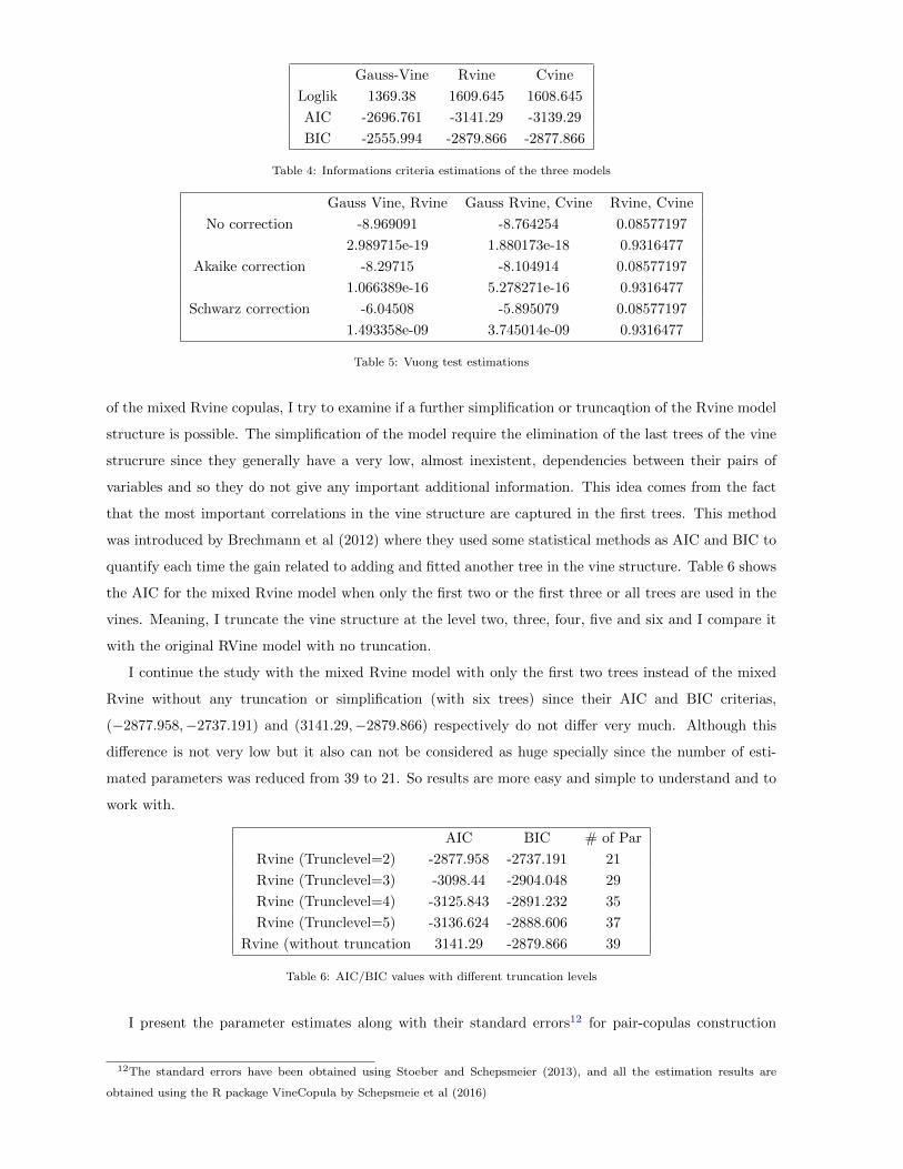
Gauss-Vine Rvine Cvine

Loglik 1369.38 1609.645 1608.645

AIC -2696.761 -3141.29 -3139.29

BIC -2555.994 -2879.866 -2877.866

Table 4: Informations criteria estimations of the three models

Gauss Vine, Rvine Gauss Rvine, Cvine Rvine, Cvine

No correction -8.969091 -8.764254 0.08577197

2.989715e-19 1.880173e-18 0.9316477

Akaike correction -8.29715 -8.104914 0.08577197

1.066389e-16 5.278271e-16 0.9316477

Schwarz correction -6.04508 -5.895079 0.08577197

1.493358e-09 3.745014e-09 0.9316477

Table 5: Vuong test estimations

of the mixed Rvine copulas, I try to examine if a further simplification or truncaqtion of the Rvine model

structure is possible. The simplification of the model require the elimination of the last trees of the vine

strucrure since they generally have a very low, almost inexistent, dependencies between their pairs of

variables and so they do not give any important additional information. This idea comes from the fact

that the most important correlations in the vine structure are captured in the first trees. This method

was introduced by Brechmann et al (2012) where they used some statistical methods as AIC and BIC to

quantify each time the gain related to adding and fitted another tree in the vine structure. Table 6 shows

the AIC for the mixed Rvine model when only the first two or the first three or all trees are used in the

vines. Meaning, I truncate the vine structure at the level two, three, four, five and six and I compare it

with the original RVine model with no truncation.

I continue the study with the mixed Rvine model with only the first two trees instead of the mixed

Rvine without any truncation or simplification (with six trees) since their AIC and BIC criterias,

(−2877.958,−2737.191) and (3141.29,−2879.866) respectively do not differ very much. Although this

difference is not very low but it also can not be considered as huge specially since the number of esti-

mated parameters was reduced from 39 to 21. So results are more easy and simple to understand and to

work with.

AIC BIC # of Par

Rvine (Trunclevel=2) -2877.958 -2737.191 21

Rvine (Trunclevel=3) -3098.44 -2904.048 29

Rvine (Trunclevel=4) -3125.843 -2891.232 35

Rvine (Trunclevel=5) -3136.624 -2888.606 37

Rvine (without truncation 3141.29 -2879.866 39

Table 6: AIC/BIC values with different truncation levels

I present the parameter estimates along with their standard errors12 for pair-copulas construction

12The standard errors have been obtained using Stoeber and Schepsmeier (2013), and all the estimation results are

obtained using the R package VineCopula by Schepsmeie et al (2016)

12

making up the mixed Rvine structure, with a truncation level equal to two, for the set of variables: SP

GSCI industrial metals, SP GSCI precious metals, SP GSCI agriculture, SP GSCI energy, SP500, MSCI

China index and MSCI India index. For now I consider the whole period from 01/1993 to 01/2016 (table

7)but then I will be studying the dependence in different sub-samples to account for different phenomenon

in the period of study . The estimated parameters are in all cases statistically significant at 5% percent

level. The tree given by the best fitted Vine structure to the data is given below and results of the

estimation are given in table 7.

Figure 5: The first and the seconf trees of the RVine structure estimated in table 7

The first tree of the Vine represents the maximal spanning tree for the unconditional bivariate correla-

tions (Kendall’s tau). The degree of dependencies gets smaller each time I add a tree which is a common

feature of Vine models where the correlations is concentrated mostly in the first tree also characterized

by unconditinal dependence contrarily to conditional dependence in the remaining trees. The first tree

indicates that there are two potential central variables: precious metals commodity and industrial metals

commodity. The SP500 is only joined with the industrial metals indice. The MSCI China is correlated

positively to the industrial metals among all commidity sectors and the indian equity depend on the chi-

neese equity, no relation with any commodity has been detected. The Kendall’s tau measures between the

different pairs of the variables and for both tress are not very high but positive. So dependence between

the different commodities and the SP500 stock indice is not very strong when we consider this long period

of time . Dependence is more important when in-between different commodity sectors than whith stock

markets. Although there is an exception. The co-movement between industrial metals and both the

SP500 and MSCI equities does exist and is positive. Considering the whole period of study, one can say

that even though the dependence is low, it does exist mostly between the four commodity sectors. The

SP 500 appears only on one pair over the four that construct the first tree (and one pair over three in the

second tree). Similarily with the chineese equity only linked to one sector. Thus, equities and commodity

markets tend to show, overall, no relation instead of having negative correlation as confirmed by some

authors. Thus correlation between commodities and equities is relatively low when treating the whole

sample. In fact, Byksahin and Robe (2011) showed that dependency between commodities and equities

did not increase until 2008. In addition, the positive dependence between industrial metals commodities

13

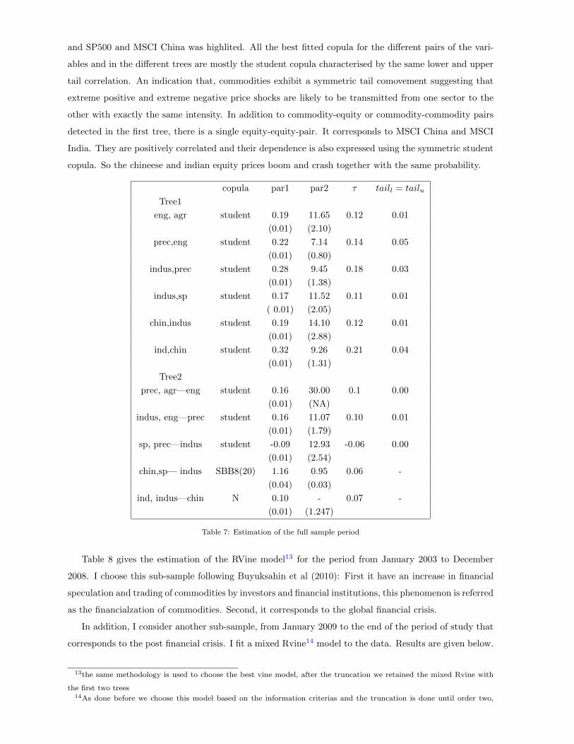
and SP500 and MSCI China was highlited. All the best fitted copula for the different pairs of the vari-

ables and in the different trees are mostly the student copula characterised by the same lower and upper

tail correlation. An indication that, commodities exhibit a symmetric tail comovement suggesting that

extreme positive and extreme negative price shocks are likely to be transmitted from one sector to the

other with exactly the same intensity. In addition to commodity-equity or commodity-commodity pairs

detected in the first tree, there is a single equity-equity-pair. It corresponds to MSCI China and MSCI

India. They are positively correlated and their dependence is also expressed using the symmetric student

copula. So the chineese and indian equity prices boom and crash together with the same probability.

copula par1 par2 τ taill = tailu

Tree1

eng, agr student 0.19 11.65 0.12 0.01

(0.01) (2.10)

prec,eng student 0.22 7.14 0.14 0.05

(0.01) (0.80)

indus,prec student 0.28 9.45 0.18 0.03

(0.01) (1.38)

indus,sp student 0.17 11.52 0.11 0.01

( 0.01) (2.05)

chin,indus student 0.19 14.10 0.12 0.01

(0.01) (2.88)

ind,chin student 0.32 9.26 0.21 0.04

(0.01) (1.31)

Tree2

prec, agr—eng student 0.16 30.00 0.1 0.00

(0.01) (NA)

indus, eng—prec student 0.16 11.07 0.10 0.01

(0.01) (1.79)

sp, prec—indus student -0.09 12.93 -0.06 0.00

(0.01) (2.54)

chin,sp— indus SBB8(20) 1.16 0.95 0.06 -

(0.04) (0.03)

ind, indus—chin N 0.10 - 0.07 -

(0.01) (1.247)

Table 7: Estimation of the full sample period

Table 8 gives the estimation of the RVine model13 for the period from January 2003 to December

2008. I choose this sub-sample following Buyuksahin et al (2010): First it have an increase in financial

speculation and trading of commodities by investors and financial institutions, this phenomenon is referred

as the financialzation of commodities. Second, it corresponds to the global financial crisis.

In addition, I consider another sub-sample, from January 2009 to the end of the period of study that

corresponds to the post financial crisis. I fit a mixed Rvine14 model to the data. Results are given below.

13the same methodology is used to choose the best vine model, after the truncation we retained the mixed Rvine with

the first two trees14As done before we choose this model based on the information criterias and the truncation is done until order two,

14

copula par1 par2 τ taill tailu

Tree1

eng,agr SBB1(17) 0.06 1.16 0.16 0.000 0.19

(0.03) (0.03)

prec,eng student 0.30 8.78 0.2 0.05 0.05

(0.02) (2.24)

indus,prec student 0.39 14.27 0.26 0.02 0.02

(0.02) (5.35)

indus,sp rotated BB8(SBB8 20) 1.23 0.93 0.08 - -

(0.09) (0.06)

indus,chin BB1(7) 0.19 1.06 0.13 0.07 0.03

(0.04) (0.02)

ind,chin BB1(7) 0.33 1.19 0.28 0.21 0.17

(0.05) (0.03)

Tree2

prec,agr—eng F(5) 1.13 0.12 - -

(0.16)

indus,eng—prec rotated Gumbel(SG 14) 1.10 0.09 - 0.12

(0.02)

sp,prec—indus STD -0.08 12.67 -0.05 0.00 0.00

(0.03) (4.73)

chin,sp— indus C (3) 0.09 - 0.04 - 0

(0.01)

ind,indus— chin G(4) 1.04 - 0.04 0.05 -

(0.01)

Table 8: Estimation of the period 2003-2008

From both table 8 and 9, we notice that correlations (in-between equities and commodities) did

increase in the last decades from 2003 and on compared to the whole period of study. This rise was

accentuated after the crisis, however, it already begun aroud 2003 when the financialization of commodity

market have been established and markets become more integrated. Thus, the co-movements between

commodities and equities is time varying and fluctuates depending on the period considered. Delatte

and Lopez (2013) also confirmed this fact. The increase of dependence caused by the financial crisis

was highlighted and accentuated indirectly by the rise of specultions and trading of commodities in the

derivative and financial markets together with using them as a hedge for diversification benefits to improve

the risk performance of portfolios of investors. Surprisingly I found that even for the post-crisis period,

dependencies remained high (compared to table 7 (whole period)) and did not recover to their pre-crisis

state. Also, as before, industrial metals represents an exception compared to other sectors. It became

less dependent on the SP500 compared to the full sample (kendall tau passed from 0.11 to 0.08) and was

even replaced by the energy sector in the last sample.

In terms of the interaction and the association with the different variables that build the trees of the

vine structure , I notice that for the two sub-samples as well as for the whole period, the SP500 indice

meaning we only retain the firs two trees in the Vine

15

copula par1 par2 τ taill tailu

Tree 1

agri,eng student 0.32 9.38 0.201 0.04 0.04

(0.02) (2.37)

indus,prec student 0.37 6.26 0.240 0.11 0.11

(0.02) (1.09)

eng,indus student 0.44 6.37 0.3 0.13 0.13

(0.02) (1.10)

eng,sp student 0.45 7.26 0.3 0.12 0.12

(0.02) (1.43)

chin,indus 19 SBB7 1.22 0.23 0.19 0.05 0.24

(0.03) (0.04)

ind,chin student 0.52 16.92 0.35 0.03 0.03

(0.02) (7.40)

Tree 2

agri,indus/eng Franck 1.15 0.13 - -

(0.15)

prec,eng/indus student 0.16 6.04 0.1 0.06 0.06

(0.03) (1.05)

indus,sp/eng student 0.22 8.82 0.140 0.03 0.03

(0.02) (2.06)

chin,eng—indus 3 c 0.07 - 0.04 - 0.00

(0.01)

ind,indus—chin N 0.18 - 0.11 - -

Table 9: Estimation of the period 2009-2016

is only joined with either the industrial metals or the energy commodities. Meaning that there is a lack

of comovements and a non existant correlation between the SP500 and commodities for both sectors:

agriculture and precious metals. An indication and a confirmation of their role as a safe haven since they

can offer diversification benefits for potfolio allocation. Contrarily, energy and industrial metals sectors

are more correlated to the SP500 equity index, and so they are behaving more like traditional financial

assets and are more integrated to the SP500 than agriculture and precious metals thus can be used more

for speculation and trading purposes. Although between the two sectors, there is a difference in terms

of their interactions to the SP500. Energy sector is more correlated to the equity market, specially these

last years, than industrial metals. Thus it represents the top one in the list of commodities to speculate

with more than industrial metals.

Therefore, commodities can not be considered as a single and homogeneous class since their depen-

dencies with and co-movement with the stock market (SP500), can be low or inexistent or relatively high

depending on the sector/ group of commodity.

In contrast with the SP500, the Msci china is positively correlated with only industrial metals among

commodity groups, and that is for each period of the study (full, post and pre crisis samples). In addition

this dependence is on the rise (from 0.12 to 0.19).The positive dependence of the chineese equity market

with particularily industrial metals is rather expected. Actually, China’s growth in consumption of metals

16

has been the main driving force behind global metal consumption since the early 2000s. However the

main reason behind the co-movement between industrial metals commodity market and the chineese

equity market comes from the heavy transactions caused by speculation and massive trading volume

for investement purposes. The industrial metals is the top one in the list of commodity-trading in the

chineese. That is why its relation with this sector was the only one highlited among the other sectors in

this analysis.15

India MSCI is only correlated with china MSCI and not with any other commodity sector or the US

equity. Although it is also considered as one of the main consumption of industrial metals, trading with

it for speculation purposes in financial markets does not hold a great importance as China. And so the

prices are still only affected by fundamentals. Dependence for this last pair in the first tree of the RVINE

structure increased from 0.28 between 2003 and 2008 to 0.35 for the remaining period of study. Meaning

that those countries are expanding more and more their economic ties and their equity markets are more

integrated and dependenct of each other.

Assymetric copulas were assigned for almost all the pairs in the first tree of table 8, apart from the

pairs (eng,prec), (indus,prec) assigned to the student copula and the SP500-indus where the rotated BB8

copula, with no tail correlation, has been selected. A number of points can be presented based on the

choice of copula:

• Both price booms and price crashs at the energy or industrial metals commodities will be trans-

mitted at the precious metals commodities, with the same probability since their lower and upper

tails are equal. (and vice versa)

• SP500 and industrial metals have no tail correlation confirming the fact that industrial metals are

not very perfect for speculation although they do not offer any diversification benefits since they

are positively correlated to the equity market.

• The lower tail correlation is higher than the upper one in the case of both China-industrial metals

and China-India. So both pairs of the variables comove more when in bad situations or news than

when in good ones. Here, in the case of China, industrial metals commodities are a good alternative

for trading purposes.

In table 9, almost all copulas best fitted to the different pairs in the first tree of the Vine structure

correspond to the symmetric student copula with same tail dependency. Surprisingly, even the SP500 and

energy commodities share the student copula. Meaning that, for these pairs, their behaviour or correlation

in regard to either bad or good news in the market will be the same, so their co-movements remain

expected and not sudden even in extreme situations (great turbulance in the market, good news, shocks, a

15China become the center for both metal consumption and metal production globally from the last decade. As a result,

China is now the main consumption locus for most metals. It is considered as the top iron-ore-producing country, it also

consumes more than half of the world production of iron ore. It is the second largest producer of copper and consumes about

half of the world’s refined copper. In addition, it is the largest producer of aluminum and it consumes about half of the

world’s production of primary aluminum. It also consumes about half of the world’s smelted and refined nickel.(Commodity

Special Feature, IMF, 2015).

17

regulation . . . ). That’s why when variables are joined by the student copula they are considered less riskier

than variables with asymmetric copulas however they offer less gains. The only dependence, characterized

by the asymmetric BB7 copula, corresponds to MSCI China with industrial metals commodity sector. In

contrast to the previous period, the upper tail correlation (0.25) is higher than the lower one (0.05). It

means that they may have an important gain in bullish market more than a loss in bearish one. Again, a

confirmation that in the chineese case, industrial metals represents a very good commodity to speculate

with in China.

I found that after the crisis, the co-movements between commodities and the stock market returns

remaind high. But is it true for the whole period or was it just at the beginning and then correlation

did indeed recover to its initial state as before the crisis? Vine copula models are flexible for multivariate

dependence, however, the coeffecients of correlation obtained are static and so they can not take into

account the different changes in the structure of the dependence. For that I choose to apply the dynamic

copula model based on Patton (2006) between the SP500 and the different commodity sectors focusing my

attention only on the post-crisis period, to investigate the dynamics and evolutions of their dependencies.

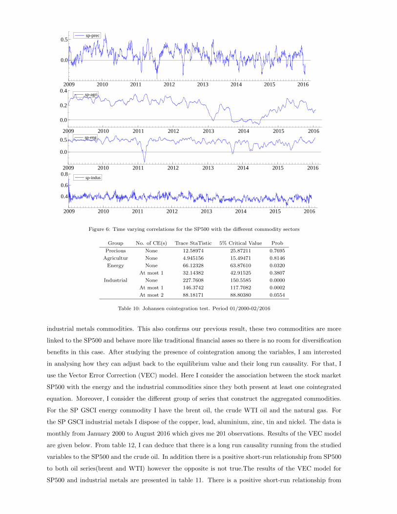
Figure 5 shows the time varying correlation given by the Gaussian copula for four pairs: the SP500 indice

with each studied sector of commodity. Obviously the comovements between each pair vary depending

on the sector. The highst correlation is given by the SP500 with energy and then with industrial metals

commodities. It corresponds to values around 0.5 for the former pair and 0.4 for the latter one. Also

apart from the agriculture commodity where there is a fall of the dependence with SP500 in the period

from end 2012 to mid 2013, correlations for the other pairs remained high years after the crisis. They did

not went back to their values before the crisis. In other words, the impact of the financial-based factors

on the volatilities of commodity price co-movement is strong during the crisis of course and remained

effective even after. The changes (rise) in dependence between commodity and the equity markets did

not decrease in the whole period considered and have not seen any turning back to its initial state.

This particular result contradicts the work of Charlot et al (2016), where they found that starting from

April 2013 commodity-equities correlation decreased compared to before. Also, both precious metals and

agriculture have the smallest correlation with SP500. So they kept their role as a safe haven.

3.4. Long run, short run equilibrium: full sample period, 2000-2016

After modelling the dependence of the series , it can be tested whether they have long-run equilibrium

or associantionship, in other words if they are cointegrated . The term cointegration can also be referred

to long-run relationship between two or more variables. In this section cointegration is examined by using

the Johansen cointegration test (Johansen, 1991). The results of this test between the SP500 price index

and the four sector of commodities (agricultural, energy, industrial metals and precious metals ) at their

levels over the period from January 2000 to February 2016 are presented in table 10. SP500 does not

exhibit any long-run relationship with agricultural and precious commodities. Which emphasis their role

as a safe haven as was confirmed in the previous section. Commodities in these two sectors can thus offer

diversification benefits to reduce the risk related to portfolios allocation. For the remaining commodities,

I found that there is two cointegration equations between the SP500 and the industrial metals and only

one with the energy commodities. Meaning that SP500 has long-run equilibrium with both energy and

18

sp-agri

2009 2010 2011 2012 2013 2014 2015 2016

0.0

0.2

0.4sp-agri

sp-eng

2009 2010 2011 2012 2013 2014 2015 2016

0.0

0.5 sp-eng

sp-indus

2009 2010 2011 2012 2013 2014 2015 2016

0.4

0.6

0.8sp-indus

sp-prec

2009 2010 2011 2012 2013 2014 2015 2016

0.0

0.5sp-prec

Figure 6: Time varying correlations for the SP500 with the different commodity sectors

Group No. of CE(s) Trace StaTistic 5% Critical Value Prob

Precious None 12.58974 25.87211 0.7695

Agricultur None 4.945156 15.49471 0.8146

Energy None 66.12328 63.87610 0.0320

At most 1 32.14382 42.91525 0.3807

Industrial None 227.7608 150.5585 0.0000

At most 1 146.3742 117.7082 0.0002

At most 2 88.18171 88.80380 0.0554

Table 10: Johansen cointegration test. Period 01/2000-02/2016

industrial metals commodities. This also confirms our previous result, these two commodities are more

linked to the SP500 and behave more like traditional financial asses so there is no room for diversification

benefits in this case. After studying the presence of cointegration among the variables, I am interested

in analysing how they can adjust back to the equilibrium value and their long run causality. For that, I

use the Vector Error Correction (VEC) model. Here I consider the association between the stock market

SP500 with the energy and the industrial commodities since they both present at least one cointegrated

equation. Moreover, I consider the different group of series that construct the aggregated commodities.

For the SP GSCI energy commodity I have the brent oil, the crude WTI oil and the natural gas. For

the SP GSCI industrial metals I dispose of the copper, lead, aluminium, zinc, tin and nickel. The data is

monthly from January 2000 to August 2016 which gives me 201 observations. Results of the VEC model

are given below. From table 12, I can deduce that there is a long run causality running from the studied

variables to the SP500 and the crude oil. In addition there is a positive short-run relationship from SP500

to both oil series(brent and WTI) however the opposite is not true.The results of the VEC model for

SP500 and industrial metals are presented in table 11. There is a positive short-run relationship from

19

the SP500 to industrial metal commodities (aluminium, copper, nickel, zinc). There is also a lack of

short-run relationship running from industrial metal commodities to the SP500.

Error Correction: D(SPC) D(ALC) D(COPC) D(LEADC) D(NIKC) D(TINC) D(ZINCC)

CointEq1 −0.029530 −0.017652 −0.236620 −0.102100 −2.614517 −0.292850 −0.005971(0.0297)∗ (0.4826) (0.0123)∗ (0.0018)∗ (0.0000)∗ (0.2816) (0.8680)

CointEq2 −0.036034 −0.097043 −0.263236 −0.238369 1.529866 −0.728253 −0.037270(0.0494)∗ (0.0047)∗ (0.0389)∗ (0.0000)∗ (0.0041)∗ (0.0484)∗ (0.4432)

D(SPC(-1)) −0.040314 0.334658 1.120200 0.316843 7.081373 1.802493 0.422384

(0.5877) (0.0164)∗ (0.0311)∗ (0.0763) (0.0011)∗ (0.2289) (0.0339)∗

D(ALC(-1)) 0.083859 0.256038 0.429158 0.088554 −1.118497 3.093669 −0.104149(0.1445) (0.0172)∗ (0.2818) (0.5190) (0.4992) (0.0079)∗ (0.4951)

D(COPC(-1)) 0.023413 0.045955 0.626494 0.130154 1.560065 0.393255 0.083040

(0.1563) (0.1350) (0.0000)∗ (0.0011)∗ (0.0012)∗ (0.2362) (0.0595)

D(LEADC(-1)) −0.009798 −0.107485 −0.591645 0.138449 0.275008 0.630933 −0.129189(0.7681) (0.0834) (0.0110)∗ (0.0831) (0.7743) (0.3458) (0.1453)

D(NIKC(-1)) 0.000141 −0.005938 −0.015763 −0.012311 0.436342 −0.028065 0.002215

(0.9561) (0.2132) (0.3755) (0.0456)∗ (0.0000)∗ (0.5856) (0.7450)

D(TINC(-1)) 0.000711 −0.008141 −0.055566 −0.043650 −0.336590 0.009775 −0.035876(0.8697) (0.3137) (0.0663) (0.0000)∗ (0.0077)∗ (0.9108) (0.0022)∗

D(ZINCC(-1)) −0.045643 0.006258 −0.674406 −0.156289 −4.924479 −1.841588 0.334107

(0.2341) (0.9300) (0.0119)∗ (0.0895) (0.0000)∗ (0.0177)∗ (0.0012)∗

C 6.813226 4.208801 19.94758 10.11557 38.72142 37.71474 8.072030

(0.0909) (0.5734) (0.4748) (0.2935) (0.7383) (0.6407) (0.4505)

DUMMY −22.04503 −42.14226 −65.53297 −31.01874 −394.7327 157.6600 −30.81707(0.0669) (0.0599) (0.4313) (0.2803) (0.2545) (0.5132) (0.3345)

Table 11: VEC model for SP500 and industrial metals

3.5. long-run, short run equilibrium: post-pre crisis (2000- 07 /2007;08 /2007-2016)

The results of the cointegration test and the VEC model given for the whole period of study (2000-

20016) can be considerably improved and treated in more details if we consider sub-samples taking into

account the global financial crisis. Tables 13 and 14 show the results of the Johansen cointegration

test (based on the trace statistic and the Eigen value statistic ) between the stock market (SP500)

and different commodities in the energy sector (oil brent, crude oil and natural gas) for post-pre crisis

periods. The results indicate the presence of a long-run relationship between the SP500 and the energy

sector commodities but only for the period during/after the financial crisis and not before. This long-run

relation is to be expected since in this period there were an increase in dependence for energy commodities

as well as the stock market as was explained in the previous section leading the series to behave in the same

way. Also since the subprime crisis was global, it affected different markets, so both energy commodities

and the SP500 converged and thus exhibited long-run relationship.

The result of VECM for SP500 and energy commodities are presented in the Table 15 for the time

period from 2007 to 2016, the only period where we found cointegration. There is a single long run

associationship between the SP500 and the WTI crude oil. In addition, there is a short-run relationship

20

Error Correction: D(SP) D(OILWTI) D(OILB) D(GAS)

CointEq1 −0.012712 −0.001735 −0.001000 0.000196

(0.0201)∗ (0.0011)∗ (0.0700) (0.0261)

D(SP(-1)) 0.011756 0.013723 0.015794 0.000112

(0.8700) (0.0482)∗ (0.0310)∗ (0.9231)

D(SP(-2)) −0.102096 0.001202 0.001845 0.000456

(0.1619) (0.8637) (0.8024) (0.6977)

D(OILWTI(-1)) 2.291751 0.341644 0.169978 −0.016435(0.2157) (0.0557) (0.3642) (0.5813)

D(OILWTI(-2)) 3.120909 0.067484 0.049431 0.002342

(0.0998) (0.7104) (0.7962) (0.9387)

D(OILB(-1)) −0.575177 0.012990 0.189040 0.013121

(0.7461) (0.9394) (0.2941) (0.6470)

D(OILB(-2)) −2.510094 0.052583 −0.021831 0.012355

(0.1614) (0.7597) (0.9040) (0.6683)

D(GAS(-1)) 0.741257 0.242890 0.380511 0.002848

(0.8727) (0.5853) (0.4172) (0.9696)

D(GAS(-2)) −1.626192 −0.509363 −0.375592 0.031349

(0.7248) (0.2523) (0.4225) (0.6739)

C 3.552246 −0.025816 −0.010684 −0.003517(0.3500) (0.9436) (0.9778) (0.9542)

Table 12: VEC estimations for SP500 and energy commodities

running from SP500 to only WTI oil as well. The strong link between oil and stock market was highlited

and confirmed for this period. Also the dummy variables here, a representative for outliers and breaks,

is statistically significant. It means that, turmoils and instability along this time period did affect the

oil (brent and WTI) in the short-run. Although it is also a part of the energy class, natural gas price

behaves differently from oil. It is not affected by the stock market nor the sudden changes in the market.

Data Trend None None Linear Linear Quadratic

Test Type No Intercept Intercept Intercept Intercept Intercept

No Trend No Trend No Trend Trend Trend

Trace 0 0 0 0 0

Max-Eig 0 0 0 0 0

Table 13: Johansen cointegration test for energy commodities. Period 01/2000-07/2007

I now consider the industrial metals. I will be working with the commodity variables belonging to

this sector (aluminium, copper, lead, nickel, tin, zinc) with the SP500 to asess their relationship during

before and after the subprime crisis. The results of the Johansen test for cointegration for both periods

are given below (tables 16 and 18). Cointegration exists between the set of variables and for the two

sub-samples. So the VEC model is applied for both periods.

Results of the VEC model for the first subsample between industrial metals and SP500 are given in

table 17. Only Nickel and zinc exhibit a long-run relationship with the SP500 price. Thus SP500 and

the industrial metals commodities do not have a close relation or association over the period from 2000

21

Data Trend None None Linear Linear Quadratic

Test Type No Intercept Intercept Intercept Intercept Intercept

No Trend No Trend No Trend Trend Trend

Trace 1 1 2 3 4

Max-Eig 1 1 1 2 4

Table 14: Johansen cointegration test for energy commodities . Period 08/2007-08/2016

to 2007. Also, there is a single short run relation running from the SP500 to the aluminium. In fact,

the short-run relationships running from SP500 to industrial metals have declined from four for the full

sample (table 11) to one in this period. An indication that the effect of the financialization of commodities

phenomenen on the interdependency and co-movements between the stock market and industrial metal

market was mainly highlited in the second period of study. Table 19 shows the results of the VEC model

for the period from 07-2007 to 20016 (the after crisis). Similarly to the previous period of study, SP500

is linked and associated to both nickel and zinc. However, it exhibites a short-run relation instead of

the long-run one. Meaning that equities represented here by the SP500 have a strong link with both

zinc and nickel independently of the period of study.Apart from these two commodities, industrial metals

commodities and equitiy market are not dependent on each other in the short run as their coeffecients are

not significant. Also, the number of short-run relationships between industrial metals commodities (apart

from pairs of the variables and its regressor) was greater than during the first sub period indicating that

during and after the financial crisis, industrial metals commodities are moving together and are more

dependent in the short run.

22

Error Correction D(SP) D(OILWTI) D(OILB) D(GAS)

CointEq1 0.002880 -0.000264 -0.000158 1.09E-05

[ 3.09340]∗ [-2.64804]∗ [-1.53720] [ 1.21440]

D(SP(-1)) -0.160028 0.024154 0.020066 0.000933

[-1.49935] [ 2.11395]∗ [ 1.70812] [ 0.90447]

D(SP(-2)) -0.225654 0.009038 0.005220 0.000882

[-2.05446]∗ [ 0.76866] [ 0.43181] [ 0.83116]

D(OILWTI(-1)) 1.654350 0.309029 0.135223 -0.015831

[ 0.80258] [ 1.40043] [ 0.59602] [-0.79480]

D(OILWTI(-2)) 0.032277 -0.048070 -0.045156 0.000870

[ 0.01532] [-0.21316] [-0.19476] [ 0.04275]

D(OILB(-1)) 1.005828 -0.048164 0.172738 0.004048

[ 0.48366] [-0.21634] [ 0.75467] [ 0.20144]

D(OILB(-2)) -1.178291 0.106620 0.014448 0.013941

[-0.57306] [ 0.48438] [ 0.06384] [ 0.70168]

D(GAS(-1)) -5.774722 0.281146 0.779664 0.382830

[-0.52097] [ 0.23693] [ 0.63906] [ 3.57420]∗

D(GAS(-2)) 26.87519 0.901087 0.995470 -0.044313

[ 2.41525]∗ [ 0.75645] [ 0.81281] [-0.41212]

C 12.12546 0.251470 0.343461 -0.044756

[ 1.95111] [ 0.37798] [ 0.50213] [-0.74529]

DUMMY -15.30558 -4.122767 -4.077782 0.036849

[-0.91295] [-2.29714]∗ [-2.20991]∗ [ 0.22746]

Table 15: VEC model estiamtes,energy commodities, Period 08/2007-08/2016

Data Trend None None Linear Linear Quadratic

Test Type No Intercept Intercept Intercept Intercept Intercept

No Trend No Trend No Trend Trend Trend

Trace 2 3 3 2 2

Max-Eig 2 3 3 3 2

Table 16: Johansen cointegration test for industrial metals. Period 01/2000-08/2007

23

Error Correction: D(SPC) D(ALC) D(COPC) D(LEADC) D(NIKC) D(TINC) D(ZINCC)

CointEq1 -0.007684 0.016035 0.052974 0.028757 -4.026170 -0.063780 0.172274

[-0.29382] [ 0.36661] [ 0.30488] [ 0.92984] [-4.70739]∗ [-0.32967] [ 2.11320]∗

CointEq2 0.007907 -0.011086 -0.059035 0.004235 2.435058 0.088392 -0.104942

[ 0.47734] [-0.40019] [-0.53644] [ 0.21618] [ 4.49507]∗ [ 0.72135] [-2.03241]∗

D(SPC(-1)) -0.062778 0.417651 0.892506 0.088760 7.097824 0.475463 0.311740

[-0.54386] [ 2.16345]∗ [ 1.16380] [ 0.65024] [ 1.88022] [ 0.55681] [ 0.86638]

D(ALC(-1)) -0.027743 -0.067670 -1.628299 0.060656 -4.479157 0.411627 -0.455345

[-0.30076] [-0.43865] [-2.65701]∗ [ 0.55606] [-1.48481] [ 0.60324] [-1.58362]

D(COPC(-1)) 0.010693 -0.048433 0.424467 -0.062356 1.533436 -0.465121 0.011720

[ 0.45008] [-1.21897] [ 2.68925]∗ [-2.21948]∗ [ 1.97365] [-2.64655]∗ [ 0.15826]

D(LEADC(-1)) -0.030679 0.080042 0.323295 0.572637 -3.307473 0.100474 -0.178924

[-0.32425] [ 0.50584] [ 0.51432] [ 5.11801]∗ [-1.06892] [ 0.14355] [-0.60667]

D(NIKC(-1)) 0.001752 -0.008197 0.008484 -0.023833 0.463149 -0.042423 -0.001307

[ 0.44844] [-1.25492] [ 0.32693] [-5.15989]∗ [ 3.62588]∗ [-1.46826] [-0.10736]

D(TINC(-1)) 0.014159 0.039115 0.166920 0.011286 0.087315 0.385448 0.086504

[ 0.89357] [ 1.47599] [ 1.58556] [ 0.60230] [ 0.16849] [ 3.28826]∗ [ 1.75131]

D(ZINCC(-1)) 0.028803 0.152840 -0.348731 -0.063850 -2.994896 -0.335597 0.529540

[ 0.63704] [ 2.02125]∗ [-1.16093] [-1.19417] [-2.02542]∗ [-1.00337] [ 3.75720]∗

DUMMY -30.55327 -17.33241 229.3193 9.417137 -718.3827 229.8622 8.418020

[-1.63295] [-0.55390] [ 1.84478] [ 0.42561] [-1.17403] [ 1.66073] [ 0.14433]

Table 17: VEC model estiamtes,industrial metals, Period 2000-2007

Data Trend None None Linear Linear Quadratic

Test Type No Intercept Intercept Intercept Intercept Intercept

No Trend No Trend No Trend Trend Trend

Trace 1 2 2 2 2

Max-Eig 1 1 2 1 1

Table 18: Johansen cointegration test for industrial metals. Period 2007-2016

24

Error Correction: D(SPC) D(ALC) D(COPC) D(LEADC) D(NIKC) D(TINC) D(ZINCC)

CointEq1 -0.038397 0.056079 0.060059 -0.051777 -0.522776 0.280000 -0.027409

[-3.24802]∗ [ 2.61423]∗ [ 0.73588] [-1.58274] [-1.70735] [ 0.96810] [-1.05558]

D(SPC(-1)) -0.022599 0.297071 1.137517 0.222436 5.361612 2.371140 0.469014

[-0.22394] [ 1.62225] [ 1.63270] [ 0.79651] [ 2.05125]∗ [ 0.96037] [ 2.11589]∗

D(ALC(-1)) 0.203848 0.036232 0.653732 -0.140098 1.270299 2.476010 0.028776

[ 2.44215]∗ [ 0.23921] [ 1.13443] [-0.60652] [ 0.58757] [ 1.21244] [ 0.15695]

D(COPC(-1)) 0.025841 0.125386 0.605130 0.274278 1.105560 0.839508 0.118436

[ 1.04153] [ 2.78508]∗ [ 3.53288]∗ [ 3.99492]∗ [ 1.72043] [ 1.38304] [ 2.17331]∗

D(LEADC(-1)) 0.024315 -0.083636 -0.765243 -0.051135 1.548082 0.544222 0.007376

[ 0.49867] [-0.94526] [-2.27327]∗ [-0.37897] [ 1.22580] [ 0.45620] [ 0.06887]

D(NIKC(-1)) 0.004871 -0.004582 0.001274 0.022858 0.104850 -0.001465 -0.002601

[ 0.94024] [-0.48734] [ 0.03562] [ 1.59440] [ 0.78137] [-0.01155] [-0.22860]

D(TINC(-1)) 0.000910 -0.016020 -0.091677 -0.059599 -0.317251 -0.077638 -0.036159

[ 0.17292] [-1.67725] [-2.52289]∗ [-4.09182]∗ [-2.32709]∗ [-0.60289] [-3.12759]∗

D(ZINCC(-1)) -0.205893 0.003844 -0.137997 -0.253490 -2.031677 -1.614047 -0.042215

[-2.57806]∗ [ 0.02652] [-0.25028] [-1.14699] [-0.98218] [-0.82605] [-0.24065]

DUMMY 12.53212 -97.49007 -205.3721 -35.94123 286.7858 -52.46474 -31.52780

[ 0.64903] [-2.78239]∗ [-1.54060] [-0.67263] [ 0.57343] [-0.11106] [-0.74336]

Table 19: VEC model estiamtes,industrial metals, Period 2007-2016

25

4. Risk Management Analysis

In this section, using a risk management related analysis, a value at risk study, I demonstrate the

efficiency of the vine copula compared to other classical approach used to calculate the VAR measure,

here I will be working with the variance-covariance method. I consider a portfolio composed of the SP500

index, the Eurostoxx 50 index, oil futures contracts and gold futures contacts with equal wights (25%).

The data is monthly from January 1992 to 2002.

To determine the distribution of the portfolio returns, I will use a standard approach, the variance-

covariance. And i will compare it to the Vine approach modeling the dependence structure between the

returns in this paper: the vine copula. In a first step I investigate the marginal distributions of the

four variables. A fit of the normal distribution to the return the Eurostoxx price returns gives a mean

µ = 0.009427699 and a standard deviation s = 0.05232169. For oil futures returns, µ = 0.00950917

and s = 0.04122601, for the SP500 price returns, µ = −0.000647475 and s = 0.03422436. Finally,

the parameters µ and s correspond to 0.001509128 and 0.0863478 respectively for the case of the gold

futures. To make sure that the gaussian distribution provides an appropriate fit to the returns, I apply

the Kolmogorov-Smirnov goodness-of-fit test. The pvalues given by the test for the SP500 returns, gold

futures returns, oil futures returns, Eurostox 50 returns are 0.2541, 0.9164, 0.506 and 0.7777 respectively.

Thus, the null hypothesis of the test can not be rejected. The normal distribution is an appropriate fit

to the marginal return series. As mentioned above, I will be comparing two approaches using the VaR

measure: the Vine copula model used in this paper VS the standard multivariate gaussian or variance-

covariance approach that is usually applied in portfolio management.

For the variance-covariance approach, only the variance-covariance matrix of the returns need to be

estimated. Then, based on the potfolio weights, the mean of the marginals and the variance-covariance

matrix, we obtain the joint distribution of the potfolio with a mean equal to 0.001058664 and a standard

deviation equal to 0.05504472. The 95”%, 99% and 99.9% Value-at-Risk (VaR) measures of the portfolio

distribution based on the variance-covariance method are reported in the following Table. In the next

step, I use the Vine copula model to specify the multivariate distribution of the returns of the portfolio.

After determinig the Vine copula parameters for the data I simulate a new data based on the same

estimated vine structure . The obtained four variables are uniform so they need to be transformed onto

return series by applying the inverse distribution function. At the end the return of the portfolio is the

sum of these new data taking into account the different wights. The VaR measures of this portfolios for

both approaches are then computed and given in the following table.

The kurtosis is higher for the model using Vine copula, further more there is a negativ skeweness in

the data that is only detected by the same model. Which for investors can mean a greater chance of

extremely negative outcomes. Also both V aR0.95 and V aR0.99 are higher for the Vine copula case. So

the covariance-variance approach based on the multivariate normal distribution underestimate the risk

compared to the Vine approach. These results, along with those presented in the previous section could

be of great help for investors and financial institutions for risk management or hedging purposes as well

as portfolio optimisation.

26

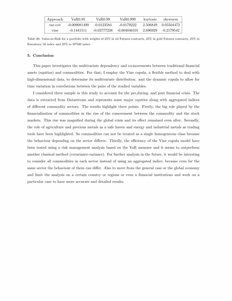
Approach VaR0.95 VaR0.99 VaR0.999 kurtosis skewness

var-cov -0.009081499 -0.0123584 -0.0179222 2.506849 0.05504472

vine -0.1441511 -0.02777238 -0.004046101 2.696929 -0.2179542

Table 20: Value-at-Risk for a portfolio with weights of 25% in oil Futures contracts, 25% in gold Futures contracts, 25% in

Eurostoxx 50 index and 25% in SP500 index.

5. Conclusion

This paper investigates the multivariate dependency and co-movements between traditional financial

assets (equities) and commodities. For that, I employ the Vine copula, a flexible method to deal with

high-dimensional data, to determine its multivariate distribution. and the dynamic copula to allow for

time variation in correlations between the pairs of the studied variables.

I considered three sample in this study to account for the pre,during, and post financial crisis. The

data is extracted from Datastream and represents some major equities along with aggregated indices

of different commodity sectors. The results highlight three points. Firstly, the big role played by the

financialization of commodities in the rise of the comovement between the commodity and the stock

markets. This rise was magnified during the global crisis and its effect remained even after. Secondly,

the role of agriculture and precious metals as a safe haven and energy and industrial metals as trading

tools have been highlighted. So commodities can not be treated as a single homogeneous class because

the behaviour depending on the sector differes. Thirdly, the efficiency of the Vine copula model have

been tested using a risk management analysis based on the VaR measure and it seems to outperform

another classical method (covariance-variance). For further analysis in the future, it would be intersting

to consider all commodities in each sector instead of using an aggregated indice, because even for the

same sector the behaviour of them can differ. Also to move from the general case or the global economy

and limit the analysis on a certain country or regions or even a financial institutions and work on a

particular case to have more accurate and detailed results.

27

Appendix

5.1. The decomposition of multivariate distributions

I begin with an itroduction concerning the copulas theory before explaining the decomposition of

multivariate distributions. The last step is to introduce the theory behind the Vine that enable us to

determine the dependence.

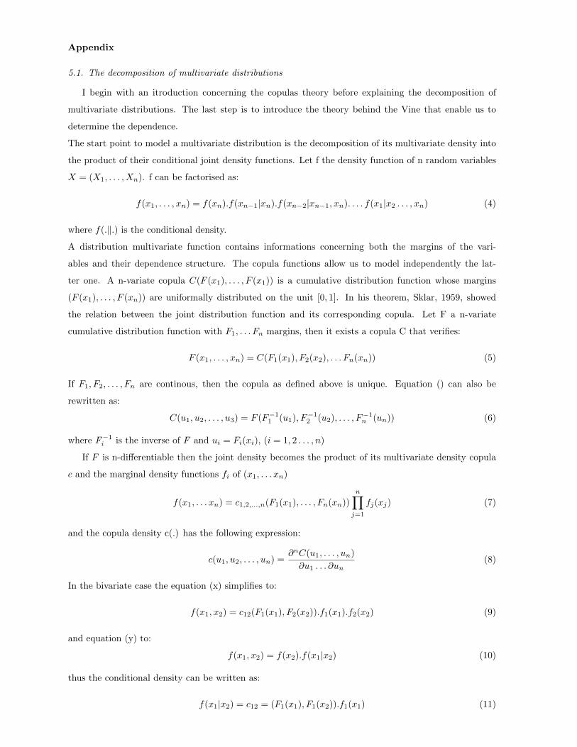
The start point to model a multivariate distribution is the decomposition of its multivariate density into

the product of their conditional joint density functions. Let f the density function of n random variables

X = (X1, . . . , Xn). f can be factorised as:

f(x1, . . . , xn) = f(xn).f(xn−1|xn).f(xn−2|xn−1, xn). . . . f(x1|x2 . . . , xn) (4)

where f(.‖.) is the conditional density.

A distribution multivariate function contains informations concerning both the margins of the vari-

ables and their dependence structure. The copula functions allow us to model independently the lat-

ter one. A n-variate copula C(F (x1), . . . , F (x1)) is a cumulative distribution function whose margins

(F (x1), . . . , F (xn)) are uniformally distributed on the unit [0, 1]. In his theorem, Sklar, 1959, showed

the relation between the joint distribution function and its corresponding copula. Let F a n-variate

cumulative distribution function with F1, . . . Fn margins, then it exists a copula C that verifies:

F (x1, . . . , xn) = C(F1(x1), F2(x2), . . . Fn(xn)) (5)

If F1, F2, . . . , Fn are continous, then the copula as defined above is unique. Equation () can also be

rewritten as:

C(u1, u2, . . . , u3) = F (F−11 (u1), F−12 (u2), . . . , F−1n (un)) (6)

where F−1i is the inverse of F and ui = Fi(xi), (i = 1, 2 . . . , n)

If F is n-differentiable then the joint density becomes the product of its multivariate density copula

c and the marginal density functions fi of (x1, . . . xn)

f(x1, . . . xn) = c1,2,...,n(F1(x1), . . . , Fn(xn))

n∏j=1

fj(xj) (7)

and the copula density c(.) has the following expression:

c(u1, u2, . . . , un) =∂nC(u1, . . . , un)

∂u1 . . . ∂un(8)

In the bivariate case the equation (x) simplifies to:

f(x1, x2) = c12(F1(x1), F2(x2)).f1(x1).f2(x2) (9)

and equation (y) to:

f(x1, x2) = f(x2).f(x1|x2) (10)

thus the conditional density can be written as:

f(x1|x2) = c12 = (F1(x1), F1(x2)).f1(x1) (11)

28

If we consider three random variables X1, X2, X3 then

f(x1|x3, x2) =f(x1, x3|x2)

f(x3|x2)=c1,3|2(F (x1|x2), F (x3|x2))f(x1|x2)f(x3|x1)

f(x3|x2)

= c1,3|2(F (x1|x2), F (x3|x2))f(x1|x2)

= c1,3|2(F (x1|x2), F (x3|x2))c1,2(F1(x1), F2(x2))f1(x1)

(12)

where c12|3 is the copula that corresponds to the variables:F (x1|x3) and F (x2|x3) and thus the 3 di-

mensional joint density can be represented, as the following, in terms of bivariate copulas C12,C23,C13|2

corresponding to the cdensities, c12, c23 and c13|2, that is the pair-copulas. The choice of each one is

independenct from the others it depends only on the dependence structurte of the variables.

f(x1, x2, x3) = f(x3).f(x2|x3).f(x1|x2, x3)

= c12(F1(x1), F2(x2)).c23(F2(x2), F3(x3).c13|2(F1|2(x1|x2), F3|2(x3|x2)).

3∏j=1

f(xi)

(13)

This is one of the possible representation to express the joint density using the product of its copulas

densities and marginals. Where a multivariate copula can be built using a cascade of bivariate copulas ,

the pair coplas. It was Joe (1996) who introduced the pair copula construction method. In the general

case for n varibles, the density function f(x1, x2, . . . , xn) can be expressed as:

f(x1, x2, . . . , xn) = f(xn)f(xn−1|xn)f(x1|x2, . . . , xn) (14)

More generally any conditional marginal distribution can be written as the following :

f(xi|ν) = cxiνj |ν−j(F (xi|ν−j), F (νj |ν−j)).f(xi|ν−j) (15)

νxi+1, . . . , xn is called the conditionning set of the marginal distribution of xi and νj represents a variable

of ν, νj is the set of variables ν minus the set νj . The marginal distributions on the right side of equation

(x) can be decomposed as shown in equation (y). f(x1, f(x2), . . . xn) corresponds to the product of

bivariate density copulas and the marginal densities of the variables. This result is referred to as the pair

copula construction of f(x1, x2, . . . x3). Based on the latter equations, the decomposition (not unique) of

the joint distribution function of 4 variables could then be expressed as follows:

f1234(x1, x2, x3, x4) = f1(x1).f2|1(x2|x1).f3|1,2(x3|x1, x2).f4|123(x4|x1, x2, x3)

which can be developed to

f1234(x1, x2, x3, x4) = f1(x1)c12(F (x1), F (x2))f2(x2).c23|1(F (x2|x1), F (x3|x1))

.c13(F (x1), F (x3)).c34|12(F (x3|x1, x2), F (x4|x1, x2))c24|1(F (x2|x1), F (x4|x1))

.c14(F (x1), F (x4))f4(x4)

(16)

and finally to:

f1234(x1, x2, x3, x4) = c12(F (x1), F (x2)).c13(F (x1), F (x3))c14(F (x1), F (x4))

.c23|1(F (x2|x1), F (x3|x1)).c24|1(F (x2|x1), F (x4|x1)

.c34|12(F (x3|x1, x2), F (x4|x1, x2))

4∏i=1

fi

29

There are different ways to express the joint distributions depending on the pair copulas decom-

positions for example we have 3 decompositions for 3 dimensional distributions, 24 for 4 dimensional

distributions, 120 decompositions for 5 dimensions etc. In general it corresponds to n(n − 1)/2 for n-

dimensional distribution. To obtain a final result of the pair copula construction abtained we claerly

need to evaluate the pair copula of the conditional distribution functions of the form F (x|ν) where ν

represents the set of conditioning variables. Knowing the ν−j is the set ν minus the jth variables, one

can write the expression of F (x|ν) based on Joe (1997) as follows and referred to as the h-function by

Aas et al (2009).

F (x|ν) = h(x, v,Θ)

=∂Cx,νj |ν−j(F (x|ν−j), F (νj |ν−j))

∂F (νj |ν−j)(18)

where Θ is the set of parameters for the copula of the joint distribution function of x and ν. If ν is

univariate then we have:

Fx|ν =∂Cxν∂Fν

(19)

5.2. vines

For high dimensions there is an extremely large number of possibilities and decompositions to construct

the multivariate distribution. That’s why to build pair copulas with the most easiest way and to be able

to classify them I refer to Bedford and Cooke (2001, 2002) who introduced a method based on graphical

models called regular Vine. Later Kurowicka and Cooke and kurowicka and Joe (2011) further explained

it and the Vine pair copula construction become a flexible approach to model multivariate distributions.

Rvine decompositions encompasses many other models. And several types of vines have been proposed

in the literature. I focus in the next section on two subsets of the Rvine: the Canonical vines and

the Dvine. Vines are graphical models to model dependence with high dimensional data. They were

introduced by Bedford and Cooke (2002). Graphically speaking, in a Vine tree, nodes corresponds the

random variables, and edges correspond to the conditional bivariate dependence between two nodes.

Thus, a Vine of n variables is a nested set of trees where the edges of the jth tree become the nodes of the

following tree j + 1 for j = 1 . . . n− 1. A vine is called regular (RVine) if two edges of tree j that become

nodes in tree j+1 and are joined in the same tree(j+1), share a common node in tree j. As mentionned

above, we focus on two type of vines: Cvine and Dvine which are the most common vines.

5.2.1. Regular Vine

I give a global overviw about regular vines which are the general form of vine and encompasses C-

vine and D-vine. This notion was introduced Bedford and Cooke (2002). Vines copulas are hierarchical

graphical model that decompose a n-dimensional joint copula density into a product of n(n-1)/2 bivariate

copulas densities. They offer a great flexibility since the bivariate copulas can take any copula type within

all the different copula families. For multivariate Gaussian copulas for example, the only copula allowed

to measure dependence between pairs of variables is the normal which does not take into account the

structure and the pattern of the data. The bivariate unconditional copulas for each pair of variables are

30

also called pair-copulas, that’s why based on a graphical model the vine, the model is often referred to

as a pair-copula construction (PCC).

Regular vine copulas can be considered as an ordered sequence of trees, where j refers to the number

of the tree and a bivariate unconditional copula c(.|.) is assigned to each of the n - j edges of tree j

(Bedford and Cooke).

Using the regular vine copula models one can construct a wide variety of flexible multivariate copulas

because each of the n(n − 1)/2 building blocks (or pair-copulas) can be chosen arbitrarily as explained

above. Moreover, a pair-copula construction does not suffer from the curse of dimensions because it

is build upon a sequence of bivariate unconditional copulas which renders it very attractive for high-

dimensional applications. Thats why in terms of flexibility, the vine based on the pair copula construction

are the best option.

An R-vine V specifies a factorization of a copula density c(x1, x2, . . . , xn) connected with a tree Tm =

{Vm, Em},m = 1, 2, . . . n − 1. A a regular vine tree sequence is constructed as a particular nested set

trees as the following:

• Let T1, . . . Tn−1 be the trees in an R-Vine V connecting the sequence of pair copulas with a set of

nodes Vi and set of edges Ei. As an example, the first tree has a set of nodes V1 = 1, . . . , n with a

set of edges E1.

• Every edge e ∈ Ei has associated three sets of variable indexes N(e), C(e), D(e) ⊂ 1, . . . , n called

the constraint, conditioned and conditioning sets of E, respectively.

• In the first tree T1, any edge e ∈ E1 joining nodes j, k ⊂ V1, C(e) = N(e) = {j, k} and D(e) = {∅}.

• Whenever two nodes in Ti+1 are joined by an edge, the corresponding edges in Ti must share a

common node. (Proximity condition)

• Edges e = (e1, e2) ∈ Ei have conditioned, conditioning and constraint sets given by C(e) =

N(e1)∆N(e2), D(e) = N(e1) ∩N(e2) and N(e) = N(e1) ∪N(e2) where A∆B = (A B) ∪ (B A).

Each of the edges in the trees T1, . . . , Td−1 forming the vine V corresponds to a different conditional

bivariate copula density that build the joint density c(u1, . . . , un). For n-variables there are a total of

n(n−1)/2 edges. In other words, c(u1, . . . , un) can be factorized to n(n−1)/2factors. So one can wonder

how to obtain the form of these factors. For any edge e(j, k) ∈ Ti with conditioned set C(e) = {j, k} and

conditioning set D(e) we define cjk|D(e) to be the bivariate copula density for uj and uk given the value

of the conditioning variables {ui, i ∈ D(e)}, that is:

cjk|D(e) = c(F (uj |ui, i ∈ D(e)), F (uk|ui, i ∈ D(e))) (20)

where F (uj |ui, i ∈ D(e)) and F (uk|ui, i ∈ D(e)) are conditional cdf of uj and uk respectively given

the value of the conditioning variables ui, i ∈ D(e). Then, the vine V formed by the hierarchy of trees

31

T1, . . . , Tn−1 has density given by:

c(u1, . . . , un) =∏n−1i=1

∏e(j,k)∈Ei

cjk|D(e) (21)

. =∏n−1i=1

∏e(j,k)∈Ei

cjk|D(e)(Fj|D(uj |uD(e)), Fk|D(uk|uD(e))) (22)

(23)

An example of an R-vine tree sequence for n=5 is given in Figure 5. It shows a construction of an

5-dimensional regular vine structure with a density f(x1, x2, . . . , x5) with the product of 10 bivariate

conditional copula densities. The first tree T1 has nodes V1 = {1, 2, 3, 4, 5}. {1, 4|3} for example represents

the edges {{1, 3}, {4, 3}. The union of this edge is {1, 3, 4} since 1 ∈ {1, 3} ∈ {{1, 3}, {4, 3} and

4 ∈ {4, 3} ∈ {{1, 3} , {4, 3}}. Also, since {1, 3} ∩ {4, 3} = {3}, then {3} is the conditioning set, and

{1} , {4} are the conditioned sets. The density the Regular vine copula that corresponds to the tree

sequence in Figure 5 can be written as:

f(x1, . . . , x5) = c1,2(x1, x2)c13(x1, x3)c34(x3, x4)c35(x3, x5)

.c23|1(x2|1, x3|1)c14|3(x1|3, x4|3)c15|3(x1|3, x5|3)

.c2,4|13(x2|13, x4|13)c45|13(x4|13, x5|13)c25|134(x2|134, x5|134)

(24)

1 2

3

4 5

1,2

1,3

3,4 3,5 1,5;3

1,4;3

2,3;1 2,4;1,3

4,5;1,3

T1 T2 T3 T4

1,2

1,3

3,53,4

2,3;1

1,5;31,4;

3

2,4;1,3

4,5;

1,3

2,5

;1,3

,4

Figure 7: Example of a regular vine tree sequence.

To search for the appropriate Rvine tree structure, the different pair copula families that construct it

and their corresponding parameters, I refer to the method of Dissmann et al (2013) summarized in the

following table.

5.2.2. D-vines and C-vine

I will consider two subsets called C-vine, and D-vine. I refer to the work of Aas et al to illustrate

and explain these models. A regular vine is considered a cvine if in the each tree of the vine structure

there exists a unique node (for each considered tree) called the root node where all the variables in the

considered tree have their pairwise dependence with the root node modeled using a bivariate copulas each

time. The canonical vine models are caracterised by a star structure. A joint probability multivariate

32

density function, corresponding to a cvine is given by:

f(x1, . . . , xn) =

n∏k=1

fk(xk).

i=1∏d−1

j=1∏d−i

cj,j+i|1...j−1(Fj|1...j−1(xj |x1, . . . , xj−1),

Fi+j|1...j−1(xi+j |x1, . . . , xj−1))

(25)

where j < i, the index i corresponds to the trees and j to the edges. Each tree Ti has a unique node

that is connected to the n− i edges. Here the outer product runs over the n− 1 trees and root nodes i,

while the inner product refers to the d− i pair copulas in each tree i = 1 . . . , d− 1. F (|) and f(.) denote

conditional distribution functions and the joint density respectively. A C-vine is preferable when there

is a key variable that governs the interactions of other variable.

The joint density function of the 5 varibles given bu the cvine representation is expressed as follws:

f12345 = f1(x1)f2(x2)f3(x3)f4(x4)f5(x5)

.c12(F1(x1), F2(x2))c13(F1(x1), F3(x3))c14(F1(x1), F4(x4))c15(F1(x1), F5(x5))

.c23|1(F (x2|x1), F (x3|x1))c24|1(F (x2|x1), F (x4|x1))c25|1(F (x2|x1), F (x5|x1))

.c34|12(F (x3|x1, x2), F (x4|x1, x2))c35|12(F (x3|x1, x2), F (x5|x1, x2))

.c45|123(F (x4|x1, x2, x3), F (x5|x1, x2, x3))

(26)

Similarly, the construction of Dvine is based on the choice of a specefic order of the studied variables. For

a dvine structure, each edge is associated with a pair-copula density used to model dependence between

the two variables that share this edge. In other words for the first tree, I model the dependence of the first

and second variables together using a pair copula and we do the same for the remainning variables (the

third and forth variables together etc). The same principle applies for all the trees forming the dvine. I

notice in this case that there is no need for a root variable in each tree like in the cvine. The dependence

of the variables are not revolving around one variable. And every node is only related to two edges. The

33

Figure 8: C-vine with 5 variables, 4 trees and 10 edges

d-dimensional D-vine density, given by Bedford and Cooke (2001), is:

f(x1, . . . , xn) =

n∏k=1

fk(xk).

i=1∏d−1

j=1∏d−i

ci,i+j|i+1,...,i+j−1(Fi|i+1,...,i+j−1(xi|xi+1, . . . , xi+j−1),

Fi+j|i+1,...,i+j−1(xi+j |xi+1, . . . , xi+j−1))

(27)

Below, a 5-dimensional D-vine structure is presented:

to which corresponds the following joint density:

f12345 = f1(x1)f2(x2)f3(x3)f4(x4)f5(x5)

.c12(F1(x1), F2(x2))c23(F (x2), F (x3))c34(F (x3, x4))c45(F (x4), x5)

.c13|2(F (x1|x3), F (x3|x2))c24|3(F (x2|x3), F (x4|x3))c35|4(F (x3|x4), F (x5|x4))

.c14|23(F (x1|x2, x3), F (x4|x2, x3))c25|34(F (x2|x3, x4), F (x5|x3, x4))

.c15|234(F (x1|x2, x3, x4), F (x5|x2, x3, x4))

(28)

34

Figure 9: A D-vine with 5 variables, 4 trees and 10 edges

Bibliographiee

• Abe Sklar, (1959), Fonctions de repartition a n dimensions et leurs marges., Institut de Statistique de

l’Universite de Paris, 8:229231

• Andrew Patton, (2006), Modelling asymmetric exchange rate dependence, International Economic Re-

view, Vol. 47, No. 2,

• Anna Creti, Marc Joets, Valrie Mignon, (2013), On the links between stock and commodity markets’ volatil-

ity, Energy Economics, Volume 37, May 2013, Pages 1628

• Annastiina Silvennoinen, Susan Thorp, (2013), Financialization, crisis and commodity correlation dynamics,

Journal of International Financial Markets, Institutions and Money, vol. 24, issue C, pages 42-65

• Harry Joe (1996), Families of m-variate distributions with given margins and m(m-1)/2 bivariate

dependence parameters, IMS lecture Notes, Distributions with fixed marginals and related topics, pp. 120141

• Tim Bedford, Roger Cooke (2001), Probability Density Decomposition for Conditionally Dependent Ran-

dom Variables Modeled by Vines, Annals of Mathematics and Artificial Intelligence,32(1), 245268.

• Tim Bedford, Roger Cooke, (2002), Vines - a New Graphical Model for Dependent Random Variables,

The Annals of Statistics, 30(4), 10311068

• Byksahin Bahattin, Michael Haigh , Michel Robe , (2010), Commodities and equities: Ever a market of one?,

Journal of Alternative Investments, 7695

• Kyongwook Choi , Shawkat Hammoudeh, (2010), Volatility behavior of oil, industrial commodity and stock

markets in a regime-switching environment, Energy Policy 38, 43884399

• C Genest, B Rmillard, D Beaudoin, (2009), Goodness-of-fit tests for copulas: A review and a power study,

Insurance: Mathematics and economics 44 (2), 199-213

• Charles Jones, Gautam Kaul, (1996), Oil and the Stock Markets, THE JOURNAL OF FINANCE VOL, LI.

NO, 2 JUNE 1996

35

• James Chong , Joelle Miffre , (2010), Conditional correlation and Volatility in Commodity Futures and

Traditional Asset Markets, Journal of Alternative Investments, 61-75.

• Dissmann J, Brechmann E, Czado C, Kurowicka D, (2013), Selecting and estimating regular vine copulae

and application to financial returns., Computational Statistics & Data Analysis, 59:5269

• Eric Jondeau, Micheal Rockinger, (2006), The Copula-GARCH Model of Conditional Dependencies: An

International Stock Market Application, Journal of International Money and Finance, 25, 827853

• Paul Embrechts , Giovanni Puccetti , (2010), Risk Aggregation. Copula Theory and its Applications, Lecture

Notes in Statistics - Proceedings 198, Springer Berlin/Heidelberg, pp. 111-126

• Brechmann E., Claudia Czado, Aas K., (2012), Truncated regular vines in high dimensions with application

to financial data, Canadian Journal of Statistics 40(1):68 - 85

• Claude B. Erb ,Campbell R. Harvey, (2006), The Strategic and Tactical Value of Commodity Futures,

Financial Analysts Journal, Volume 62, Number 2

• Drew Creal, Siem Jan Koopman, Andr Lucas, (2008), Generalized autoregressive score models with appli-

cations, Journal of applied econometrics, Volume 28, Issue 5

• Franois Lescaroux , Valrie Mignon, (2008), On the influence of oil prices on economic activity and other macroeco-

nomic and financial variables, OPEC energy review, Volume 32, Issue 4,Pages 343380

• Gideon Boako, Paul Alagidede, (2016), Global commodities and African stocks: A ’market of one?’, Inter-

national Review of Financial Analysis,Volume 44, Pages 226237

• Gary Gorton, K. Geert Rouwenhorst, (2006), Facts and Fantasies about Commodity Futures, Financial

Analysts Journal, Volume 62, Issue 2

• Shawkat Hammoudeh, Huimin Li, (2008), Sudden changes in volatility in emerging markets: The case of

Gulf Arab stock markets, International Review of Financial Analysis, 17(1), 47-63.

• Ing-Haw Cheng, Wei Xiong, (2014), Financialization of Commodity Markets, Annual Review of Financial

Economics, Vol. 6, 419-441

• K Aas, C Czado, A Frigessi, H Bakken, (2009), Pair-copula constructions of multiple dependence, Insurance:

Mathematics and economics 44 (2), 182-198

• Ke Tang, Wei Xiong, (2012), Index Investment and the Financialization of Commodities, Financial Analysts

Journal, Volume 68, Number 6

• Mehmet Fatih ztek, Nadir cal, (2017), Financial crises and the nature of correlation between commodity

and stock markets, International Review of Economics and Finance, 5668

• Mohamed El Hedi Arouri, Jamel Jouini, Duc Khuong Nguyenc, (2012), On the impacts of oil price fluctuations

on European equity markets: Volatility spillover and hedging effectiveness, Energy Economics 34 (2),

611-617

• Aristidis K. Nikoloulopoulos, Harry Joe, Haijun Li (2012). Vine copulas with asymmetric tail dependence

and applications to financial return data, Computational Statistics and Data Analysis 56(11), 36593673.

• Nobuyoshi Yamori, (2011), Co-Movement between Commodity Market and Equity Market: Does Com-

modity Market Change?, Modern Economy, 2011, 2, 335-339

• Philippe Charlot, Olivier Darne, Zakaria Moussa, (2016), Commodity returns co-movements: Fundamentals

or style effect?, Journal of International Money and Finance, Volume 68, November 2016, Pages 130160

36

• Paul Embrechts, Filip Lindskog, Alexander McNeil, (2001), Modelling Dependence with Copulas and Appli-

cations to Risk Management, Department of Mathematics, ETHZ

• Robert Engle, (2002), Dynamic Conditional Correlation:A Simple Class of Multivariate Generalized

Autoregressive Conditional Heteroskedasticity Models, Journal of Business & Economic Statistics, Vol. 20,

No. 3

• Soren Johansen, (1991), Estimation and Hypothesis Testing of Cointegration Vectors in Gaussian Vector

Autoregressive Models, Econometrica Vol. 59, No. 6, pp. 1551-1580

• Suleyman Basak,Anna Pavlova, (2016),A Model of Financialization of Commodities The Journal of Finance,

VOL LXXI, NO 4

• Shaun K. Roache, (2012), Chinas Impact on World Commodity Markets, IMF Working Paper

• Ulf Schepsmeier, (2016), Package ’VineCopula’, R cran

• Vlayoudom Marimoutou, Manel Soury, (2015), Energy markets and CO2 emissions: Analysis by stochastic

copula autoregressive model, Energy journal, Volume 88, Pages 417-429

37