multiuser receiver design - nc state universityhdai/mimomud_section1_v8.pdf · multiuser receiver...
TRANSCRIPT

Multiuser Receiver Design
Huaiyu Dai, Sudharman Jayaweera, H. Vincent Poor, Daryl Reynolds, Xiaodong Wang
1 Introduction
The preceding chapter considered the design of receivers for MIMOsystems operating as single-user
systems. Increasingly however, as noted in Chapters 2 and 4, wireless communication networks operate
as shared-access systems in which multiple transmitters share the same radio resources. This is due
largely to the ability of shared access systems to support flexible admission protocols, to take advantage
of statistical multiplexing, and to support transmission in unlicensed spectrum. In this chapter we will
extend the treatment of Chapter 5 to consider receiver structures for multiuser, and specifically, multiple-
access MIMO systems. We will also generalize the channel model considered to include more general
situations than the flat-fading channels considered in Chapter 5. To treat these problems, we will first
describe a general model for multiuser MIMO signaling, and then discuss the structure of optimal receivers
for this signal model. This model will generally include several sources ofinterference arising in MIMO
wireless systems, including multiple-access interference caused by the sharing of radio resources noted
above, inter-symbol interference caused by dispersive channels, and inter-antenna interference caused by
the use of multiple transmit antennas. Algorithms for the mitigation of all of these types of interference
can be derived in this common framework, leading to a general receiver structure for multiuser MIMO
communications over frequency-selective channels. As we shall see, these basic algorithms will echo
similar algorithms that have been described in Chapters 3 and 5. Since optimal receivers in this situation
are often prohibitively complex, the bulk of the chapter will focus on useful lower complexity sub-optimal
iterative and adaptive receiver structures that can achieve excellentperformance in mitigating interference
in such systems. This discussion is organized as follows.
1
Section 2 of this chapter will introduce a simple, yet useful, model for the signals received by
the receiver in a MIMO system. This model is rich enough to capture the important behavior of most
wireless communication channels, while being simple enough to allow for the straightforward motivation
and understanding of the basic receiver elements arising in practical situations. This section also derives
a canonical multiuser MIMO receiver structure, discusses several specific receivers that can be explained
within this structure, and provides a digital receiver implementation that will be useful in the discussion
of adaptive systems later in the chapter.
As noted above, complexity is a major issue in multiuser receiver design and implementation, and
the remainder of this chapter addresses the problem of complexity reductionin multiuser MIMO systems.
This complexity takes two forms: computational, or implementational, complexity; and informational
complexity.
The first type of complexity refers to the amount of resources needed to implement a given
receiver algorithm. Optimal MIMO multiuser receiver algorithms are typically prohibitively complex in
this sense, and thus a major issue in this area is complexity reduction. Sections 3and 4 of this chapter
address the principal method for complexity reduction in practical multiuser receivers, namely the use of
iterative algorithms in which tentative decisions are made and updated iteratively. There are a number
of basic iterative techniques, involving different tradeoffs between complexity and performance, and
depending on the type of system under consideration, and these are described in Section 3. In Section 4,
we tackle the additional complexity that arises in receiving space-time coded transmissions, such as those
described in Chapter 4, in multiuser MIMO systems. Here, iterative algorithms similar to those discussed
in Chapter 5 provide the answer to finding algorithms that can exploit the space-time coded structure with
only moderate increases in complexity.
The second type of complexity refers to the amount of knowledge that a given receiver needs to
have about the structure of received signals in order to effect signalreception. Although, as we will see
shortly, optimal MIMO multiuser reception requires knowledge of the waveforms being transmitted by
all users sharing the channel and the structure of the physical channel intervening between transmitters
and receiver, this type of knowledge is rarely available in practical wireless multiuser systems. Thus, it is
2

necessary to consider adaptive receiver algorithms that can operate without such knowledge, or with only
limited such knowledge. Such algorithms are the topic of Section 5 of the chapter, in which the structure
of adaptive MIMO multiuser receivers is reviewed.
The chapter will conclude in Sections 6 and 7 with a summary and pointers to additional reading
of interest in this general area.
2 Multiple-Access MIMO Systems
As noted above, this section will provide a general treatment of the multiuser MIMO receiver design
problem. Here we will focus on modeling and on the structure of optimal receivers. In doing so, we will
expose the principal issues underlying the reception of signals in multiuser MIMO systems, and also will
set the stage for more practical algorithms developed in succeeding sections.
2.1 Signal and Channel Models
In order to discuss multiuser MIMO receiver structures, it is useful to first specify a general model for
the signal received by a MIMO receiver in a multiuser environment. (See Fig. 1.) In doing so, we will
build on the signaling model developed in Chapter 1, and in particular our model is an abstraction of the
physical channel described there that is especially useful for the purposes of this chapter. Specifically, a
useful received signal model for a multiuser MIMO system havingK active users,MT transmit antennas
andMR receive antennas, and transmitting over a frame ofB symbol periods, can be written as follows:
rp(t) =K∑
k=1
MT∑
m=1
B−1∑
i=0
bk,m[i] gk,m,p(t− iTs) + np(t) , p = 1, . . . ,MR, (1)
where the various quantities are as follows:
• rp(·) = the signal received at the output of thepth receive antenna,
• bk,m[i] = the symbol transmitted by userk from itsmth antenna in theith symbol interval,
• gk,m,p(·) = the waveform on which symbols from themth antenna of userk arrives at the output
of thepth receive antenna,
3

T AP
T T
T T T AP AP
T T T T
T T
Figure 1: A Multiuser MIMO System.
• Ts = the symbol period, and
• np(·) = ambient noise at thepth receive antenna.
Each of the waveformsgk,m,p(·) can be modeled as
gk,m,p(t) =
∫ ∞
−∞sk,m(u)fk,m,p(t− u)du, (2)
where
• sk,m(·) = the signaling waveform used by userk on itsmth antenna, and
• fk,m,p(·) = the impulse response of the channel between themth transmit antenna of userk and the
pth receive antenna output.
Thus, we are assuming linear modulation and a linear channel model, both of which are reasonable
assumptions for wireless systems. Note that, sincegk,m,p(·) does not depend on the symbol indexi in this
model, we are implicitly assuming here that the channel is stable (and time-invariant) over the transmission
frame (which isBTs seconds long) and that the transmitters use the same signaling waveforms in each
symbol period. The first of these assumptions is valid for the coherence times and signaling parameters
arising in most systems of interest, while the latter is often violated, particularly in cellular systems.
4
However, with the exception of the adaptive methods of Section 5, this time variation is not difficult to
incorporate into any of the results described in this chapter, and is omitted here for the sake of notational
simplicity. (See, e.g., [46]).
In order to minimize the number of parameters in this model, we will assume that the signaling
waveforms are normalized to have unit total energy, i.e.,
∫ ∞
−∞[sk,m(t)]2 dt = 1 , k = 1, . . . ,K ,m = 1, . . . ,MT . (3)
In reality, the actual transmitted waveforms will carry differing and non-unit energies, reflecting the
transmitted powers of the various users’ terminals. However, from the vantage point ofreceiverdesign,
the critical scale parameter is the received power of a user, which will depend on the user’s transmitter
power and the gain of the intervening channel. Thus, it is convenient to lumpall scaling of the signals into
the channel impulse responsefk,m,p(·), and to simply assume normalized waveforms (3) at the transmitter.
Again, from the receiver’s point of view, it is impossible anyway to separate the effects of channel gain
and transmit power on the received power. Also for convenience, we will assume that the transmitted
waveforms have duration of only a single symbol interval; i.e.,
sk,m(t) = 0 , t /∈ [0, Ts] . (4)
As with the normalization constraint (3), this assumption does not remove any generality since received
waveforms that extend beyond a single symbol interval can be modeled via dispersion in the channel
response.
A typical and useful model for the channel response is as a discrete multipath model:
fk,m,p(t) =L∑
ℓ=1
hk,m,p,ℓ δ(t− τk,m,p,ℓ) , (5)
whereδ(·) denotes the Dirac delta function, and wherehk,m,p,ℓ andτk,m,p,ℓ ≥ 0 denote the channel gain
and propagation delay, respectively, of theℓth path of the channel between themth transmit antenna of
5

userk and the output of thepth receive antenna.1 In this case, the waveformsgk,m,p(·) are of the form
gk,m,p(t) =
L∑
ℓ=1
hk,m,p,ℓ sk,m(t− τk,m,p,ℓ) . (6)
That is, in this model, the waveform received at a given receive antennap from a given transmit antenna
m of a particular userk is the superposition ofL scaled and delayed copies of the waveformsk,m(·)
transmitted from that antenna. Except where noted otherwise, we will assume this particular model for
the channel response in the sequel.
The signaling waveformssk,m(·) can take many forms. Although these waveforms can be though
of as being generic in our discussion, a quintessential example is the case inwhich the transmitted signals
are in direct-sequence code-division multiple-access (DS/CDMA) format.This is a very widely used
signaling format in wireless systems (used notably in both major 3G cellular standards), and is the
example used in the simulations discussed in succeeding sections of this chapter. In the notation of this
section, this format can be described as follows.
DS/CDMA Signaling: In the DS/CDMA format, the signaling waveforms used by all transmitters are in
the form of spread-spectrum signals; i.e., the waveforms{sk,m(·)} of (1) are of the form
sk,m(t) =1√N
N−1∑
j=0
c(j)k,mψ(t− (j − 1)Tc) , 0 ≤ t ≤ Ts , (7)
whereN is the spreading gain of the system,c(0)k,m, c
(1)k,m, . . . , c
(N−1)k,m is the spreading code (or signature
sequence) associated with themth transmit antenna of userk, Tc = Ts/N is the chip interval, andψ(·)
is a chip waveform having unit-energy and approximate durationTc. (For a general discussion of spread-
spectrum signaling, see, e.g., [48].) In studying this format, the chip waveformψ(·) is often modeled as
a unit-energy pulse of durationTc; i.e.,
ψ(t) =
1√Tc, t ∈ [0, Tc]
0 , otherwise. (8)
1For simplicity, we lump the effects of the radio channel itself and the antennaresponse into the same termhk,m,p,ℓ. Often
these two terms can be separated (see, e.g., [46]). However, no generality is lost in lumping these effects together for the purposes
of analysis and exposition.
6
Again, most of the results of this chapter apply to general signaling waveforms, and it is not
necessary to particularize to this specific format except where noted. Itshould also be mentioned that
these signaling waveforms, the symbols, the noise, and the channel responses may be taken to be complex
(rather than real as is tacitly assumed here). We will not need this generalityhere until Section 5, and so
we will defer discussions of needed modifications (which are minor) until then. A complex version of
the above model can be found in [46], which allows for two-dimensional signaling constellations, such
as QPSK and QAM, to fit within this model.
As an additional assumption, we assume that the ambient noise processesnp(·) , p = 1, . . . ,MR,
are mutually independent white Gaussian processes with common spectral heightσ2.We also assume that
the transmitted symbols take values in a finite alphabetA containing|A| elements. Beginning in Section
3, we will specialize this to the binary antipodal caseA = {−1,+1}. This is primarily for convenience,
as most of the results in this chapter hold for more general signaling alphabets.
Finally, we note thatMT , B andL in the above model could vary from user to user, whileL
could also vary from antenna pair to antenna pair. However, again for simplicity, we will assume them
to be constants, as the extensions of the discussions in the chapter to these non-constant cases are quite
straightforward.
2.2 Canonical Receiver Structure
A basic MIMO multiuser receiver structure can be usefully decomposed intotwo parts: a front-end
(or hardware) part, and a decision algorithm (or software) part. In practice, these pieces may not be
completely distinct, as much of the front-end may be implemented in software; but for the purposes of
exposition, it is a useful decomposition.
A canonical front-end for such a system can be derived based on thetheory of statistical inference.
In particular, it is of interest to examine the so-calledlikelihood functionof the observations (1) given
the collection of transmitted symbol:{bk,m[i]}k=1,...,K; m=1,...,MT ; i=0,...,B−1 . Due to the assumption of
white, Gaussian noise, the logarithm of this likelihood function is given (up to ascalar multiple) by the
7

Cameron-Martin formula [29] to be:
K∑
k=1
MT∑
m=1
B−1∑
i=0
bk,m[i]zk,m[i] − 1
2
K∑
k,k′=1
MT∑
m,m′=1
B−1∑
i,i′=0
bk,m[i]bk′,m′ [i′]C(k,m, i; k′,m′, i′) , (9)
where, fork = 1, . . . ,K, m = 1, . . . ,MT , andi = 0, . . . , B − 1,
zk,m[i] =L∑
ℓ=1
P∑
p=1
hk,m,p,ℓ
∫ ∞
−∞rp(t)sk,m(t− τk,m,p,ℓ − iTs)dt , (10)
and fork, k′ = 1, . . . ,K, m,m′ = 1, . . . ,MT , andi, i′ = 0, . . . , B − 1,
C(k,m, i; k′,m′, i′) =P∑
p=1
L∑
ℓ,ℓ′=1
hk,m,p,ℓhk′,m′,p,ℓ′
∫ ∞
−∞sk,m(t−τk,m,p,ℓ−iTs)sk′,m′(t−τk′,m′,p,ℓ′−i′Ts)dt .
(11)
Although the expression (9) may seem somewhat complicated, the key thing to note about it is that
the antenna outputs,r1(t), r2(t), . . . , rP (t), enter into the likelihood function only through the collection
of “observables”{zk,m[i]}k=1,...,K; m=1,...,MT ; i=0,...,B−1 . This means that this collection of variables
is a sufficient statistic[29] for making inferences about the corresponding set of transmitted symbols
{bk,m[i]}k=1,...,K; m=1,...,MT ; i=0,...,B−1 , which implies in turn that all attention can be restricted to this
set of observables when designing and building systems or algorithms for demodulating and detecting
the transmitted symbols.
Before turning to some types of algorithms that we might use for this purpose,it is worthwhile
to examine the structure of this set of observables a bit more closely. In particular, it can be seen that (10)
consists of three basic operations:
1. integration to obtain:xk,m,p,ℓ[i] =∫∞−∞ rp(t)sk,m(t− τk,m,p,ℓ − iTs)dt ;
2. correlation to obtain:yk,m,ℓ[i] =∑P
p=1 hk,m,p,ℓ xk,m,p,ℓ[i] ; and
3. summation to obtain:zk,m[i] =∑L
ℓ=1 yk,m,ℓ[i].
The first operation is amatched filteringoperation, so that we see that each received antenna
output is filtered with a filter that is matched to the waveform received on eachpath from each transmit
antenna in each symbol interval of each user. Thus, there areK ×MR × B × L ×MT matched filter
8

outputs, which we can think of as being produced by a bank of linear filters, each of which is sampled at
the end of each signaling interval; i.e., samples are taken at timesiTs for i = 0, . . . , B − 1.
The second operation, in which the matched-filter outputs{xk,m,p,ℓ[i]} are correlated across the
receive antenna array with the channel/antenna gains{hk,m,p,ℓ} , can be viewed as a form ofbeamforming,
through which the spatial dimension afforded by the receive array is exploited. Since the termshk,m,p,ℓ
also incorporate channel gains, this is not strictly a simple beamforming operation in general, but it has a
similar effect of coherently collapsing the spatial dimension of the array. Note that, after beamforming,
there areK ×B × L×MT observables.
Finally, the third operation, in which the beamformer outputs{yk,m,ℓ[i]} are added, is amultipath
combiner, or Rake operation through which the spatial dimension introduced by the multipath channel is
exploited. Typically a Rake receiver also includes a correlation with the channel multipath coefficients.
This is being done here as part of the beamforming operation. So, the combination of the second and
third operation is equivalent to beamforming followed by Rake combining, andthis combination might
be decomposed in other ways in practice. After this third operation, there areK ×MT ×B observables,
one for each symbol in the frame of each user.
These three operations constitute the (hardware) front-end of a canonical multiuser receiver, as
illustrated in Fig. 2. This front-end is sometimes known as aspace-time matched filter.Note that,
although this structure may seem complicated, it is essentially composed of standard communication-
system components: matched filters, beamformers, Rake receivers.
... ...
Temporal Matched
Filters {k,m,l,p}
Decision Logic
110 … 010 …
011 …
Beam Formers {k,m,l}
RAKEs { k,m }
... ...
... ...
... ...
... ...
K K M M T T L L M M R R K K M M T T L L K K M M T T
iT iT s s
... ...
Temporal Matched
Filters {k,m,l,p}
Decision Logic
110 … 010 …
011 …
Beam Formers {k,m,l}
RAKEs { k,m }
... ...
... ...
... ...
... ...
K K M M T T L L M M R R K K M M T T L L K K M M T T
iT iT s s
Figure 2: A Canonical MIMO Multiuser Receiver Structure.
It is noteworthy that this formalism and general front-end structure encompasses three standard
interference-mitigation problems in communications. To discuss this point, it is useful to define the
9
parameter
∆ =
⌈maxk,m,p,ℓ {τk,m,p,ℓ}
Ts
⌉, (12)
where⌈x⌉ denotes the smallest integer not less thanx. ∆ is the maximum delay spread of the wireless
channels (5) in units of symbol intervals, and is thus the maximum extent to whichsymbols of a given user
interfere with one another. Returning to the general receiver structure, the case in whichK = MT = 1
and∆ > 1 is the channel equalization problem studied notably in the 1970s; the caseMT = ∆ = 1 and
K > 1 is the traditional multiuser detection problem, studied notably in the 1980s; and finally the case
in whichK = ∆ = 1 andMT > 1 is the standard MIMO communications problem, exemplified by the
BLAST architecture studied notably in the 1990s. Combinations of these problems and refinements on
them have been mainstays of research and development in digital communications throughout the past few
decades and continuing to the present day. The applicability of the results inthis chapter to these various
problems, both individually and jointly, is worth keeping in mind in the subsequent discussions. Thus, the
receiver architectures described herein can be applied other than in themultiuser MIMO communications
setting, and many of them generalize solutions to the more particular cases noted above.
2.3 Basic MUD Algorithms
As illustrated in Fig. 2, theKMTB outputs of the canonical multiuser front-end are operated upon by a
decision algorithm whose purpose is to infer the values of theKMTB transmitted symbols{bk,m[i]} .This
decision algorithm can take many forms, ranging through the full toolbox of statistical signal processing:
optimal algorithms based on maximum-likelihood or maximuma posterioriprobability criteria, linear
algorithms, iterative algorithms, and adaptive algorithms. Each of these techniques will be discussed
briefly in the following paragraphs, and counterparts to these algorithms are discussed in Chapters 3 and
5. However, before discussing these types of algorithms, it is useful to first examine the relationship
between the observables{zk,m[i]} and the corresponding symbols{bk,m[i]} to be inferred. To do so, it is
convenient to collect the symbols into aKMTB-long column vectorb by sorting the symbols{bk,m[i]}
10
first by symbol number, then by user number, and finally by antenna number. That is,
b =
b[0]
b[1]
...
b[N − 1]
(13)
where
b[i] =
b1[i]
b2[i]
...
bK [i]
(14)
with
bk[i] =
bk,1[i]
bk,2[i]
...
bk,MT[i]
. (15)
Similarly, we can denote byz the set of observations{zk,m[i]} collected into aKMTB-long column
vector indexed conformally withb. We can also define aKMTB ×KMTB cross-correlation matrixR
whose(n, n′)-th element is given by the cross-correlationC(k,m, i; k′,m′, i′) from (11) where the indices
are determined by matching with the corresponding elements ofb (or, equivalently,z); i.e.,bn = bk,m[i]
andbn′ = bk′,m′ [i′] with n = [iK + (k − 1)]MT +m andn′ = [i′K + (k′ − 1)]MT +m′.
With these definitions, the observables and transmitted symbols can be related toone another
through the relationship
z = R b + n , (16)
wheren denotes aKMTB-long noise vector having theN(0, σ2R
)distribution. (Here,0 denotes a
KMTB-long vector having all components equal to zero.)
As a simple example, we can consider the flat-fading, synchronous case,in which all signals
arrive at the receive array with the same symbol timing. This correspondsto the discrete multipath model
of (5) withL = 1 andτk,m,p,ℓ ≡ 0.
11

fk,m,p(t) = hk,m,p,1 δ(t) . (17)
In this case, the matrixR is a block-diagonal matrix havingB identical blocks along its diagonal,
each of dimensionKMT ×KMT . These square sub-matrices contain the cross-correlations between the
signals received from the different antennas of the different users. So, for example, in this case, the first
block is given by
Rn,n′ =
∫ ∞
∞sk,m(t)sk′,m′(t)dt ×
P∑
p=1
hk,m,p,1hk′,m′,p,1 , n, n′ = 1, 2, . . . ,KMT , (18)
where the indicesn andn′ correspond, respectively, to antennam of userk and antennam′ of userk′,
both in the zeroth symbol interval. This block is then repeatedB times along the diagonal ofR. This
example is further illuminated by considering the single-receive-antenna case (MR = 1), in which this
first diagonal block simplifies to
Rn,n′ =
∫ ∞
∞sk,m(t)sk′,m′(t)dt Ak,mAk′,m′ , n, n′ = 1, 2, . . . ,KMT , (19)
withAk,m = hk,m,1,1 for k,m = 1, . . . ,K,MT , n = (k− 1)MT +m, andn′ = (k′− 1)MT +m′. This
block is thus of the form:
ARA (20)
whereA is a diagonal matrix having the received amplitudesA1,1, . . . , A1,MT, A2,1, . . . , A2,MT
, . . . , AK,1, . . . , AK,MT
on its diagonal, and whereR is thenormalizedcross-correlation matrix of the signaling multiplex:
Rn,n′ =
∫ ∞
∞sk,m(t)sk′,m′(t)dt , n, n′ = 1, 2, . . . ,KMT . (21)
For example, in the DS/CDMA case of (7)-(8), this normalized cross-matrix isgiven by
Rn,n′ =1
N
N−1∑
j=0
c(j)k,mc
(j)k′,m′ , n, n
′ = 1, 2, . . . ,KMT ; (22)
that is, the normalized cross-correlation matrix is determined by the cross-correlations of the spreading
sequences used by the system. The specific structure of this matrix depends on how the spreading
sequences are allocated to the various users’ antennas. In some systems, all antennas of the same user
12

use the same spreading code, while in others, different spreading codes are used for all antennas. As an
example, if the spreading codes are so-calledm-sequences (see, e.g., [48]), thenRn,n′ = 1 for antennas
using identical spreading codes andRn,n′ = −1/N, for antennas (and users) using different spreading
codes.
In the general case in which the channel is not flat or the users are notsynchronous, the block
diagonal form of this example becomes a block Toeplitz form, as will be discussed in Section 3. From
(16) we see that the basic relationship betweenz andb is that of a noisy linear model, and so the basic
problem to be solved by the decision algorithm in Fig. 2 is that of fitting such a model. At first glance,
this appears to be a rather straightforward problem, as the fitting of linear models is a classical problem
in statistics. However, the difficulty in this problem arises because the vectorb to be chosen in this fit has
discrete-valued elements (e.g.,±1), and this significantly increases the complexity of fitting this model
(16).
In general, the most powerful techniques for data detection are maximum-likelihood (ML) and
maximuma posterioriprobability (MAP) detection. ML detection makes inferences about the transmitted
symbols in (1) by choosing those symbol values that maximize the log-likelihood function of (9). To get
a sense of this task, it is useful to use the compact notation of (16) to rewritethe log-likelihood function
(9) as
bT z − 1
2bTRb . (23)
So, the ML symbol decision solve the optimization problem:
maxb∈B
[bT z − 1
2bTRb
], (24)
whereB = AKMT B. The optimization problem (24) is an integer quadratic program, which is knownto
be an NP-complete computational problem. Since the size of the search setB is potentially enormous at
|A|KMT B, solving this problem appears to be impossible2. However, for most practical wireless channels,
the matrixR has many zero elements which reduces the complexity of this problem significantly. In
particular, assuming that the signaling waveforms{sk,m(·)} are limited in duration to a single symbol
interval, and given the finite multipath channel model (5), the matrixR is a banded matrix, meaning that
2Typically, K might be dozens,MT several andB hundreds.
13
all of its elements are zero except on a certain number of diagonals; i.e.,Rn,n′ = 0 if |n−n′| > KMT ∆,
where again∆ is the maximum delay spread of the wireless channels (5) in units of symbol intervals (12).
This bandedness allows for a complexity reduction from the order of|A|KMT B needed to exhaustively
search for the ML solution, to the order of|A|KMT ∆ (per symbol) to search via dynamic programming
(see, e.g., [30]). Although in most wireless channels the maximum delay spread ∆ is much less than
the frame lengthB, even this reduced complexity is prohibitive for most applications as the exponent
KMT ∆ could still be fairly large in a typical situation with dozens of users, a few antennas per user,
and a few symbols of delay spread. The ML detector is sometimes referred toas the jointly optimal (JO)
detector.
MAP detection is applicable to situations in which the receiver knows a prior probability distri-
bution governing the values that the transmitted symbols may assume. In this situation, it is possible to
consider the posterior probability distribution of a given symbol, conditionedon the observations, and
to infer that value for each symbol that has maximuma posterioriprobability (APP). That is, a given
symbol, saybn is detected asbn according to the following criterion:
bn = arg
{maxa∈A
P (bn = a|z)}. (25)
Using Bayes’ formula, we can write the APP as
P (bn = a|z) =
∑b∈Bn,a
ℓ(z|b)w(b)∑
b∈B ℓ(z|b)w(b), (26)
wereBn,a denotes the subset ofB in which thenth coordinate is fixed ata, w(b) is the prior probability
of b, andℓ(y|b) denotes the likelihood function ofz givenb :
ℓ(z|b) = e(bT z − 1
2bT Rb)/σ2
. (27)
Commonly, it is assumed that the symbol vectorb is uniformly distributed in its rangeB; i.e.,
that
w(b) ≡ |A|−KMT B . (28)
This assumption is equivalent to assuming that all the symbols are independent and identically distributed
(i.i.d.) from time to time, from user to user, and from antenna to antenna, and that each symbol is chosen
14

equiprobably among the elements ofA. This assumption is not always valid, as we will discuss below.
However, when it is valid, the prior distribution drops out of the computation of the APP, and the MAP
criterion becomes:
bn = arg
max
a∈A
∑
b∈Bn,a
ℓ(z|b)
. (29)
(Note that the denominator in the APP (26) is irrelevant to the maximization since it does not depend on
the value of any individual symbol.) The MAP detector is sometimes termed the individually optimal
(IO) detector since it chooses each symbol decision according to a single-symbol criterion.
Like the ML detector, the computation of symbol decisions using (29) is generally prohibitively
complex. In particular, we note that computation of the APP for each individual symbol value involves
a summation over|A|KMT B−1 values of the symbol vector. Also like ML detection, however, this
complexity can be reduced via dynamic programming to the order of|A|KMT ∆ operations per symbol
when the channel has delay spread of∆ symbol intervals [30, 39].
As we see from the above discussion, the basic complexity of ML (JO) or MAP (IO) data detection
is quite complex, on the order of|A|KMT ∆ operations per detected symbol. So, the complexity grows
with the number of users, the number of antennas, and the channel length.It is noteworthy that this issue
is present even in the single-user (K = 1) case, the single-antenna case (MT = 1), or in the flat-fading
case (∆ = 1). Only if all of these conditions is missing do we get a simple detector structure,which
reduces in either the ML or MAP case to a simple quantization:
bn = Q(zn) , (30)
where the quantizerQ : IR → A. For example, in the case of binary antipodal symbols (A = {−1,+1}),
we takeQ to be the signum function:
Q(z) = sgn(z) =
−1 z < 0
+1 z ≥ 0. (31)
Since data detection must be performed on a relatively limited computing platform (i.e, a com-
munications receiver) at essentially the rate of data transmission (i.e., tens to thousands of kilobits per
second), it is of interest to consider alternatives to the optimal detectors described above. One family
15

of such detectors are thelinear multiuser detectors, which seek to balance the simplicity of the simple
detector (30) with the power of IO or JO detection. In linear detection, this is accomplished by first
multiplying the sufficient statisticz by a suitably chosen square matrix, and then quantizing the result:
bn = Q(vn) , (32)
where
v = Mz (33)
and whereM is aKMTB × KMTB matrix. This type of detector is illustrated in Fig. 3. Various
types of detectors can be implemented through different choices of the matrixM. Three key ones can be
described as follows.
Decision Logic
... ... = = Quantizer
Linear Transformation
(LT)
... ...
Decision Logic
... ...
Decision Logic
... ... = = Quantizer
Linear Transformation
(LT)
... ...
Quantizer Linear
Transformation (LT)
... ...
Figure 3: Linear Multiuser Algorithm.
Space-Time Matched Filter/Rake Receiver: The simplest example of a linear detector arises from choos-
ing M to be theKMTB × KMTB identity matrixI, in which case the linear detector reduces to the
simple detector of (30). This detector is a classical space-time matched filter receiver which is optimal in
an additive white Gaussian noise (AWGN) channel. A flaw of this receiveris that it addresses only the
ambient noise, while ignoring the cross-correlations between the signals affecting different symbols; i.e.,
it ignores the off-diagonal elements ofR.
Decorrelating (Zero-Forcing) Receiver: Noting from (16) that the mapping from transmitted symbols
b to the observablesz is in the form of a (square) linear transformation plus noise, a natural detection
strategy is a zero-forcing detector that eliminates the interference embodiedin the cross-correlation matrix
R. Assuming thatR is non-singular, this can be implemented as a linear detector withM = R−1. The
resulting detector is known as thedecorrelator. The decorrelator thus quantizes the variablesv = R−1z,
16
which are given by
v = b + R−1n. (34)
Note that, as expected, these transformed observables are free of (inter-user, inter-antenna, inter-symbol)
interference. However, this receiver is the opposite extreme of the matched filter receiver, in that it is
tantamount to ignoring the ambient noise to suppress the interference. Usingstandard properties of the
multivariate Gaussian distribution, the noise terms in (34) is distributed according to
R−1n ∼ N(0, σ2R−1
). (35)
Depending on the structure ofR the inverseR−1 can have very large diagonal values, leading to noise
enhancement and consequent high error rate. (This problem is well-known in the context of equalization
[33].) The assumption thatR be invertible is not overly restrictive in general, asR is at least non-negative
definite. However, there are nontrivial situations in whichR can be singular, in which case the decorrelator
is not a viable structure.
MMSE Receiver: While the matched filter addresses the ambient noise and the decorrelator addresses the
interference, the minimum-mean-square-error (MMSE) multiuser detector effects a compromise between
these two impairments by selecting the transformationM such as the vectorv = Mz is an MMSE estimate
of the symbol vectorb. For this criterion to make sense, it is necessary to provide a prior model forb.
On making the common assumption that the elements ofb are of zero mean and mutually uncorrelated,
the MMSE detector corresponds to the following choice of the matrixM :
M =(R + σ2I
)−1(36)
where, as before,I denotes theKMTB×KMTB identity matrix. Note that, it is clear from this form that
the MMSE detector represents a compromise between the matched filter (M = I) and the decorrelator
(M = R−1), in which the action of each is tempered with the action of the other. The relative mix of
these two is controlled by the noise level (or more properly by the signal-to-noise ratio (SNR), as the
signal strength is incorporated intoR). When the interference is dominant (i.e, for high SNR), the MMSE
detector mimics the decorrelator, while when the ambient noise is dominant (i.e., for low SNR) it mimics
the matched filter. More generally, it balances between these two.
17
In general, the complexity of linear multiuser detectors is that of matrix inversion, which is on the
order of(KMTB)3. As with the ML and MAP solutions, this complexity can be reduced by exploiting
bandedness in the case of short delay spread. In some cases, this complexity may also be amortized over
many frames. However, for most wireless systems, such amortization is not possible as the signaling
waveforms, the user population, or the channel parameters may change from frame to frame. Thus,
although the order of complexity here has been reduced from exponential to polynomial, complexity
is still a concern for practical systems. Moreover, in both linear and nonlinear cases, constraints on the
transmitted symbols imposed by space-time coding or temporal channel coding can add to this complexity
substantially [30].
For these reasons, a number of other techniques for multiuser reception have been developed,
with the objective of reducing computational complexity while maintaining good performance in the
presence of multiple-access interference. The principal technique fordoing this is to make use of iterative
algorithms to fit the linear model (16). This can be done either linearly with a final quantization (i.e.,
iterative linear detection), or nonlinearly with inter-iteration quantization (sometimes known as interfer-
ence cancellation). Section 3 of this chapter will address this issue in some detail for multiuser MIMO
systems. When further complexity is introduced by channel coding, iterative algorithms such as those
described in Chapter 5 (in this case “turbo” style algorithms) again allow for excellent performance with
moderate complexity. This topic is addressed in Section 4.
As noted above, another form of complexity isinformationalcomplexity, which arises from the
need to know the received waveforms{gk,m,p(·)} in the model (1) for the received signal. There are
two potential problems with this requirement. One is that the channels interveningthe transmitters and
receiver are typically dynamic and behave in a apparently random fashion. So, the channel parameters
(assuming the channel can be parameterized) are not readily known to thereceiver. Another problem is
that the signaling waveforms of all users may also not be known to the receiver, because, for example, the
receiver may only be intended to receive a subset of the users. In either case, it is thus necessary for the
receiver to be able to adapt itself to those properties of the signaling environment that it does not know.
Receiver structures for this purpose are described in Section 5 of this chapter. In preparation for this latter
18
treatment, we turn briefly, in the following sub-section, to a discrete-time model for the received signals
considered above that is more suitable for developing and discussing such adaptive receiver algorithms.
2.4 Digital Receiver Implementation
For receiver implementation, and particularly for the adaptive algorithms to bediscussed in Section 5 of
this chapter, it is useful to consider a digital representation of the signals and observables that we have
described in the preceding paragraphs. This type of representation is typically obtained by projecting
the received signals (1) onto a finite set of functions arising from a modelin which there are finitely
many degrees of freedom in the signals of interest. (Most practical signaling methods have this property.)
In this sub-section, we will particularize the above structures for this situation, and in particular will
consider the common case in which the signaling waveforms are in the DS/CDMA format, described
above and in Chapter 1. This model will then be used exclusively in Section 5of this chapter. It should
be noted, however, that similar techniques can be applied in any system allowing for a finite-degree-of-
freedom model. A notable alternative example to DS/CDMA is the case of orthogonal frequency-division
multiple-access (OFDMA) systems, in which the incoming signal can be decomposed along orthogonal
sub-carrier signals using the discrete Fourier transform (DFT).
Recall that, in the DS/CDMA format, the signaling waveforms used by all transmitters are in the
form (7). Here, we consider this format in the particular case where the chip waveform is the unit pulse
of (8). For this type of system, a natural set of observables can be obtained by projecting the received
signals of (1) onto time shifts of the chip waveformψ(·):
rp[j] =
∫ ∞
∞rp(t)ψ(t− jTs)dt =
∫ (j+1)Tc
jTc
rp(t)dt , j = 0, 1, . . . . (37)
If the system delays are all integer multiples of a chip interval (this is termed the “chip-synchronous”
case), then no information is lost in this operation, as the outputs of the matched-filter bank of Fig. 2 and
hence the sufficient statisticz can be extracted from these observables. In the chip-asynchronouscase,
inferential information may be lost in performing this operation. However, thisloss is often minimal
and the signal-processing advantages of reducing the observations to adiscrete-time sequence outweigh
this. (An alternative for the chip-asynchronous case is to integrate overshorter time intervals and thus
19

effectively to over-sample the signal; however, we will not consider this level of detail here. For further
discussion, see [46].)
As noted above, in the chip-synchronous case, the sufficient statisticz can be written as a function
of the observables{rp[j]} and thus the ML and MAP detectors are functions of these observables, as are
the linear detectors described in the preceding sub-section. In the latter case it is sometimes convenient
to combine all of the linear processing of the receiver front end and the decision algorithm of Fig. 2 into
a single linear transformation, in which case symbol detection is of the form:
bk,m[i] = Q
MR∑
p=1
∑
j
w(j)k,m,p[i]rp[j]
, (38)
where the coefficients{w
(j)k,m,p[i]
}are chosen appropriately. This structure is one that can be adapted
using standard adaptive algorithms to adjust the weighting coefficients. Although there are a number of
issues surrounding such adaptation, such as the decomposition of spatialand temporal combining, this
structure is the essence of many adaptive algorithms for multi-antenna, multiuser receiver design. An
extensive treatment of this problem can be found in [46], and we will consider particularly the MIMO
case in Section 5.
3 Iterative Space-time Multiuser Detection
Advanced signal processing such as multiuser detection, typically improvessystem performance at the cost
of computational complexity. As noted in Section 1, the optimal maximum likelihood (ML) multiuser
detector has prohibitive computational requirements for most current applications, and consequently
a variety of linear and nonlinear multiuser detectors have been proposed toease this computational
burden while maintaining satisfactory performance [38, 46]. However, inmany situations where the
combined system has large dimensions (e.g., large array size, large delay spread, large user population,
and combinations of these conditions), direct implementation of these suboptimaltechniques still proves
to be very complex. In this section, we discuss iterative techniques for efficient space-time multiuser
detection in MIMO systems [45, 8, 7]. Iterative methods are among the most practical techniques for
multiuser detection. For example, an implementation for 3G cellular systems is described in [19].
20
3.1 System Model
As noted in Section 1, we can restrict attention to the following system model (i.e.,Eq. (16)):
z = Rb + n, (39)
whereR is the cross-correlation matrix,b is the symbol vector, andn is the background noise at the input
to the decision algorithm of Fig. 2. An optimal ML space-time multiuser detector will maximize the log-
likelihood function of (23), and the computational complexity of this maximization is amajor concern,
particularly when the system dimension is large. In the following, we will use a multipath CDMA channel
for illustration purpose, but the techniques discussed can be readily applied to other equivalent MIMO
scenarios as well. In principle, the computational complexity of ML detection grows exponentially with
the size ofR, which for a multipath MIMO multiuser channel is proportional to the number of usersK,
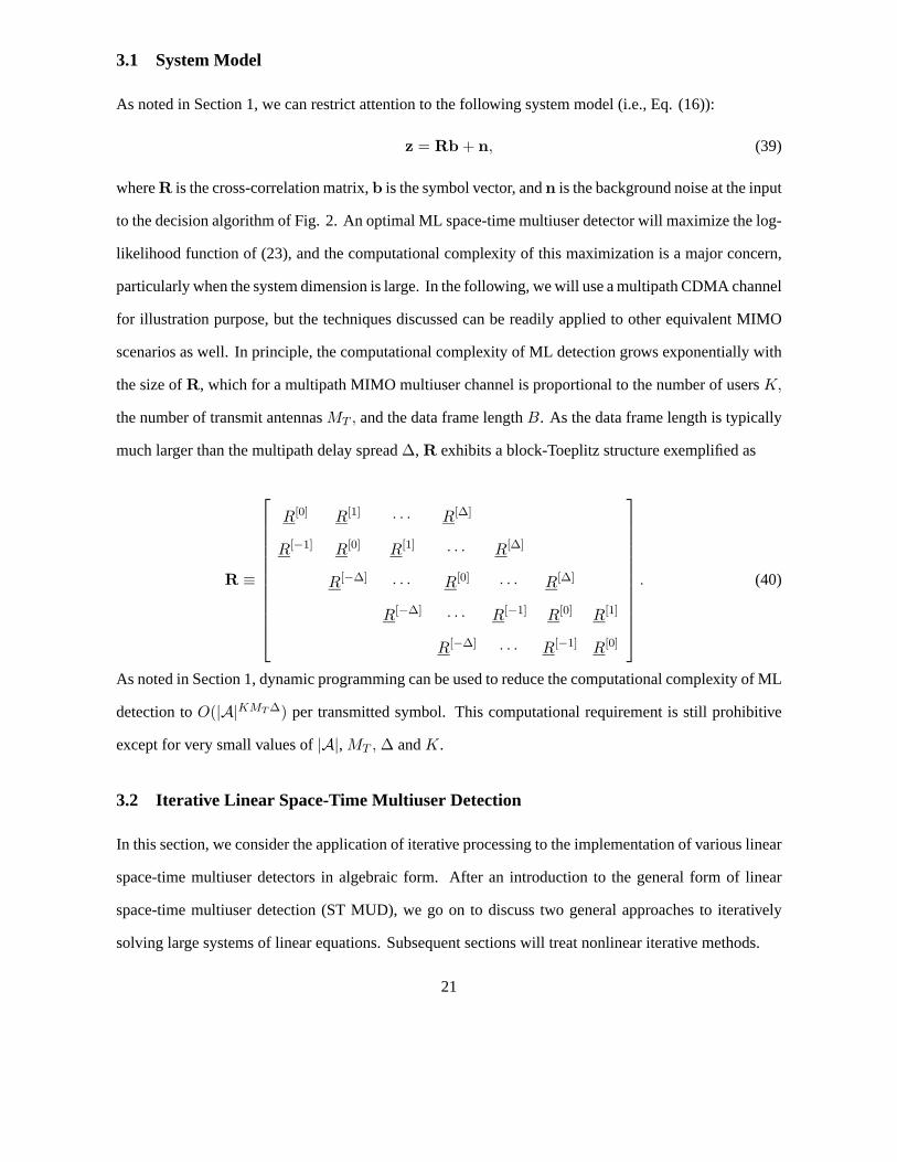
the number of transmit antennasMT , and the data frame lengthB. As the data frame length is typically
much larger than the multipath delay spread∆, R exhibits a block-Toeplitz structure exemplified as
R ≡
R[0] R[1] · · · R[∆]
R[−1] R[0] R[1] · · · R[∆]
R[−∆] · · · R[0] · · · R[∆]
R[−∆] · · · R[−1] R[0] R[1]
R[−∆] · · · R[−1] R[0]
. (40)
As noted in Section 1, dynamic programming can be used to reduce the computational complexity of ML
detection toO(|A|KMT ∆) per transmitted symbol. This computational requirement is still prohibitive
except for very small values of|A|,MT , ∆ andK.
3.2 Iterative Linear Space-Time Multiuser Detection
In this section, we consider the application of iterative processing to the implementation of various linear
space-time multiuser detectors in algebraic form. After an introduction to the general form of linear
space-time multiuser detection (ST MUD), we go on to discuss two general approaches to iteratively
solving large systems of linear equations. Subsequent sections will treat nonlinear iterative methods.
21

As noted in Section 1, linear multiuser detectors in the framework of (39) are of the form
b = sgn(Re{Mz}), (41)
whereM is a linear detection matrix. For the linear decorrelating (zero-forcing) detector, this matrix is
given by
Md = R−1, (42)
while for the linear minimum-mean-square-error (MMSE) detector, we have
Mm = (R + σ2I)−1. (43)
Direct inversion of the matrices in (42) and (43) (after exploiting the block Toeplitz structure) is of
complexityO((KMT )2B∆) per user per symbol.
The linear multiuser detection estimates of (41) can be seen as the solution of a linear equation
Cv = z, (44)
with C = R for the decorrelating detector andC = R+ σ2I for the MMSE detector. Jacobi and Gauss-
Seidel iteration are two common low-complexity iterative schemes for solving linear equations such as
(44) [14]. If we decompose the matrixC asC = CL + D + CU whereCL denotes the lower triangular
part,D denotes the diagonal part, andCU denotes the upper triangular part, then Jacobi iteration can be
written as
vm = −D−1(CL + CU )vm−1 + D−1z, (45)
and Gauss-Seidel iteration is represented as
vm = −(D + CL)−1CUvm−1 + (D + CL)−1z. (46)
From (45), Jacobi iteration can be seen to be a form of linear parallel interference cancellation, the
convergence of which is not guaranteed in general. One of the sufficient conditions for the convergence
of Jacobi iteration is thatD− (CL +CU ) be positive definite. In contrast, Gauss-Seidel iteration, which
(46) reveals to be a form of linear serial interference cancellation, converges to the solution of the linear
22

equation from any initial value, under the mild conditions thatC be symmetric and positive definite,
which is always true for the MMSE detector.
Another general approach to solving the linear equation (44) involves theuse of gradient methods,
among which are steepest descent and conjugate gradient iteration [14]. Note that solving (44) is equivalent
to minimizing the cost function
Φ(v) =1
2vHCv − vHz. (47)
The idea of gradient methods is to successively minimize this cost function along a set of directions{pm}
via
vm = vm−1 + αmpm, (48)
with
αm = pHmqm−1/p
HmCpm, (49)
and
qm = −▽Φ(v)|v=vm = z − Cvm. (50)
Different choices of the set{pm} give different algorithms. If we choose the search directionpm to be
the negative gradient of the cost functionqm−1 directly, this algorithm is the steepest descent method,
global convergence of which is guaranteed. The convergence rate may be prohibitively slow, however,
due to the linear dependence of the search directions, resulting in redundant minimization. If instead we
choose the search direction to be C-conjugate as follows
pm = arg minp∈Λ⊥
m−1
‖p − qm−1‖, (51)
whereΛm = span{Cp1, · · · ,Cpm}, then we have the conjugate gradient method, whose convergence
is guaranteed and performs well whenC is close to the identity either in the sense of being low rank
perturbation or in the sense of a norm. The computational complexity of Gauss-Seidel and conjugate
gradient iteration are similar, which is on the order ofO(KMT ∆m) per user per symbol, wherem is
the number of iterations. The numbers of iterations required by the Gauss-Seidel and conjugate gradient
methods to achieve a stable solution to the associated large system equations have been found to be on
the same order in simulations.
23
3.3 Iterative Nonlinear Space-Time Multiuser Detection
Nonlinear multiuser detectors are often based on bootstrapping techniques, which are iterative in nature.
In this section, we will consider the iterative implementation of decision-feedback multiuser detection in
the space-time domain. We also discuss briefly the implementation of multistage interference canceling
ST MUD, which serves as a reference point for introducing a new expectation-maximization (EM-) based
iterative ST MUD, to be discussed in the next subsection. For simplicity, we now restrict the signaling
alphabet to the binary antipodal set:A = {−1,+1}.
3.3.1 Cholesky Iterative Decorrelating Decision-Feedback ST MUD
Decorrelating decision feedback multiuser detection (DDF MUD) exploits the Cholesky decomposition
R = FHF, whereF is a lower triangular matrix, to determine the feedforward and feedback matrixfor
detection via the algorithm
b = sgn(F−Hz − (F − diag(F))b)). (52)
The discussion here applies readily to the implementation of MMSE decision feedback multiuser detection
as well.
Suppose we are interested in detecting symbolbn. The purpose of the feedforward matrixF−H is
to whiten the noise and decorrelate against the "future users"{sn+1, · · · , sKMT B}; while the purpose of
the feedback matrix(F − diag(F)) is to cancel the interference from "previous users"{s1, · · · , sn−1}.
Note that the performance of DDF MUD is not uniform. While the first "user"is demodulated by
its decorrelating detector, the last detected "user" will essentially achieve itssingle-user lower bound
providing the previous decisions are correct. There is another form ofCholesky decomposition, in which
the feedforward matrixF is upper triangular. If we were to use this form instead in (52), then the multiuser
detection would operate in the reverse order, as would the performance.The idea ofCholesky iterative
DDF ST MUD is to employ these two forms of Cholesky decomposition alternatively as follows.For
lower triangular Cholesky decompositionF1, first feedforward filtering is applied as
z1 = F−H1 z, (53)
24
where it is readily shown thatz1, i = F1, iibi +∑i−1
j=1 F1, ijbj + n1, i, i = 1, · · · ,KMTB, with n1,i,
i = 1, · · · ,KB, being independent and identically distributed (i. i. d.) Gaussian noise components with
zero mean and varianceσ2. We can see that the influence of the "future users" is eliminated and the noise
component is whitened. Then we use the feedback filtering to cancel the interference from "previous
users" as
u1 = z1 − (F1 − diag(F1))b, (54)
where it is easily seen thatu1,i = z1, i−∑i−1
j=1 F1, ij bj ≈ F1, iibi +n1, i, i = 1, · · · ,KMTB. Similarly,
for upper triangular Cholesky decompositionF2, we have
z2 = F−H2 z, (55)
wherez2, i = F2, iibi +∑KB
j=i+1 F2, ijbj + n2, i, i = KMTB, · · · , 1, and
u2 = z2 − (F2 − diag(F2))b, (56)
whereu2, i = z2, i−∑KMT B
j=i+1 F2, ij bj ≈ F2, iibi+n2, i, i = KMTB, · · · , 1. After the above operations
are (alternately) executed, the following log-likelihood ratio is calculated,
Li = 2Re(F∗1/2, iiu1/2, i)/σ
2, (57)
whereF1/2 andu1/2 are used to give a shorthand representation for both alternatives. Then the log-
likelihood ratio is compared with the last stored value, which is replaced by the new value if the new one
is more reliable, i.e.,
Lstoredi =
Lstoredi if |Lstored
i | > |Lnewi |,
Lnewi otherwise.
(58)
Finally we make soft decisionsbi = tanh(Li/2) at an intermediate iteration, which has been shown to
offer better performance than making hard intermediate decisions, and makehard decisionsbi = sgn(Li)
at the last iteration. Several iterations are usually enough for the system toachieve an improved steady
state without significant oscillation. The structure of Cholesky iterative decorrelating decision-feedback
ST MUD is illustrated in Fig. 4.
25

Figure 4: Cholesky iterative decorrelating decision-feedback ST MUD
The Cholesky factorization of the block Toeplitz matrixH (see (40) can be performed recursively.
For∆ = 1 we have
F =
F 1(0) 0 · · · 0 0
F 2(1) F 2(0) · · · 0 0
0
...
0 0 · · · FM (1) FM (0)
, (59)
where the element matrices are obtained recursively as follows.
V B = R[0], (60)
and, fori = B,B − 1, · · · , 1, we perform Cholesky decomposition of the reduced-rank matrixV i to get
F i(0)
V i = FHi (0)F i(0), (61)
while F i(1) is obtained as
F i(1) = (FHi (0))−1R[−1]. (62)
26
Finally we have
V i−1 = R[0] −R[1]V −1i R[−1] (63)
for use in the next iteration. The extension of this algorithm to∆ > 1 is straightforward and is omitted
here.
3.3.2 Multistage Interference Canceling ST MUD
Multistage interference cancellation (IC) is similar to Jacobi iteration except that hard decisions are made
at the end of each stage in place of the linear terms that are fed back in (45). Thus we have
bm = sgn(z − (CL + CU )vm−1) = sgn(y − (H − D)bm−1). (64)
The underlying rationale for this method is that the estimator-subtracter structure exploits the discrete-
alphabet property of the transmitted data streams. This nonlinear hard-decision operation typically results
in more accurate estimates in high SNR situations. Although the optimal decisions are a fixed point of
the nonlinear transformation (64), there are problems with the multistage IC such as a possible lack
of convergence and oscillatory behavior. In the following section we consider some improvements on
space-time multistage IC MUD. Except for the Cholesky factorization, the computational complexity for
Cholesky iterative DDF ST MUD is the same as multistage IC ST MUD, which is essentially the same
as that of linear interference cancellation, i.e.,O(KMT ∆m) per user per symbol.
3.4 EM-based Iterative Space-Time Multiuser Detection
In this section, expectation-maximization-based multiuser detection is introducedto avoid the convergence
and stability problem of the multistage IC MUD.
The EM algorithm [10] provides an iterative solution of maximum likelihood estimation problems
such as
θ(Z) = arg maxθ∈Λ
log f(Z; θ), (65)
whereθ ∈ Λ are the parameters to be estimated, andf(·) is the parameterized probability density function
of the observableZ. The idea of the EM algorithm is to consider a judiciously chosen set of "missing
27

data"W to form the complete dataX = {Z,W} as an aid to parameter estimation, and then to iteratively
maximize the following new objective function
Q(θ; θ) = E[log f(Z,W; θ)|Z = z; θ
], (66)
where it is worth emphasizing again thatθ are the parameters in the likelihood function, which are
to be estimated, whileθ representa priori estimates of the parameters from the previous iterations.
Together with the observations, these previous estimates are used to calculate the expected value of the
log-likelihood function with respect to the complete dataX = {Z,W}. To be specific, given an initial
estimateθ0, the EM algorithm alternates between the following two steps:
1. E-step, where the complete-data sufficient statisticQ(θ; θi) is computed;
2. M-step, where the estimates are refined byθi+1 = arg maxθ∈ΛQ(θ; θi).
It has been shown that EM estimates monotonically increase the likelihood, andconverge stably to an
ML solution under certain conditions [10].
An issue in using the EM algorithm is the tradeoff between ease of implementation and conver-
gence rate. One would like to add more "missing data" to make the complete data space more informative
so that the implementation of the EM algorithm is simpler than the original setting (65).However, the
convergence rate of the algorithm is inversely proportional to the Fisher information contained in the
complete data space. This tradeoff is essentially due to the simultaneous updating nature of the M-step in
the original EM algorithm [11]. Consequently, the space-alternating generalized EM (SAGE) algorithm
has been proposed in [11] to improve the convergence rate for multidimensional parameter estimation.
The idea is to divide the parameters into several groups (subspaces), with only one group being updated
at each iteration. Thus, we can associate multiple less-informative "missing data" sets to improve the
convergence rate while maintaining the overall tractability of optimization problems. For each iteration, a
subset of parametersθSiand the corresponding missing dataZSi are chosen, which is called the definition
step. Then similarly to the EM algorithm, in the E-step we calculate
QSi(θSi; θi) = E
[log f(Z,WSi ; θSi
,θiSi|Z = z; θi)
], (67)
28

whereθSi
denotes the complement ofθSiin the whole parameter set; in the M-step, the chosen parameters
are updated while the others remain unchanged as
θi+1Si
= arg maxθSi∈ΛSi
QSi(θSi; θi),
θi+1
Si
= θiSi,
(68)
whereΛSidenotes the restriction of the entire parameter space to those dimensions indexed bySi. Like
the traditional EM estimates, the SAGE estimates also monotonically increase the likelihood and converge
stably to an ML solution under appropriate conditions [11].
The EM algorithm is applied to space-time multiuser detection as follows. Supposewe would
like to detect a bitbn, n ∈ {1, 2, · · · ,KMTB}, which can be viewed as the parameter of interest, while
the interfering users’ bitsbk
= {bj}j 6=n are treated as the missing data. The complete-data sufficient
statistic is given by (Rnm is the element of matrixR at thekth row andmth column)
Q(bn; bin) =1
2σ2
−Rnnb
2n + 2bn(zn −
∑
m6=n
Rnmbm)
, (69)
with
bm = E[bm|Z = z; bn = bin
]= tanh
(Rmm
σ2(zm − Rmnb
in)
), (70)
which forms the E-step of the EM algorithm. The M-step is given by
bi+1n = arg max
bn∈ΛQ(bn; bin) =
sgn(zn −∑m6=n Rnmbm), Λ = {±1},1
Rnn(zn −∑m6=n Rnmbm), Λ = R,
(71)
whereΛ = R (the set of real numbers) means a soft decision is needed, e.g., in an intermediate stage.
Note that in the E-step (70), interference from usersj 6= n is not taken into account, since these are treated
as "missing data". This shortcoming is overcome by the application of the SAGE algorithm, where the
symbol vector of all usersb = {bj}KMT Bj=1 is treated as the parameter to be estimated and no missing data
is needed. The algorithm is described as follows: fori = 0, 1, · · · ,
1. Definition step:Si = 1 + (i mod KMTB)
2. M-step:
bi+1n = sgn(zn −∑m6=n Rnmb
im), n ∈ Si,
bi+1m = bim, m /∈ Si.
(72)
29
Note that there is no E-step since there is no missing data, and interference from all other users are
recreated from previous estimates and subtracted. The resulting receiver is similar to the multistage
interference canceling multiuser receiver (see (64)), except that thesymbol estimates are made sequentially
rather than in parallel. However, with this simple concept of sequential interference cancellation, the
resulting multiuser receiver is convergent, guaranteed by the SAGE algorithm. The multistage interference
canceling multiuser receiver discussed in 3.3.2, on the other hand, does not always converge. The
computational complexity of this SAGE iterative ST MUD is alsoO(K∆m) per user per symbol.
3.5 Simulation Results
In this section, the performance of the above described space-time multiuserdetectors is examined through
simulations on a CDMA example. We assume aK = 8-user CDMA system with spreading gainN = 16.
Each user, equipped with one single antenna, travels throughL = 3 paths before it reaches a base station
(or access point), equipped with a uniform linear arrary withMR = 3 elements and half-wavelength
spacing. The maximum delay spread is set to be∆ = 1. The complex gains and delays of the multipath
and the directions of arrival are randomly generated and kept fixed for the whole data frame. This
corresponds to a slow fading situation. The spreading codes of all users are randomly generated and kept
fixed for all the simulations.
First we compare the performance of various space-time multiuser receivers and some single-user
space-time receivers in Fig. 5. Five receivers are considered: the single-user matched filter (Matched-
Filter), the single-user MMSE receiver (SU MMSE), the multiuser MMSE receiver (MU MMSE) im-
plemented using the Gauss-Seidel or conjugate gradient iteration method (theperformance is the same
for both), the Cholesky iterative decorrelating decision-feedback multiuser receiver (Cholesky Iterative
MU DF), and the multistage interference canceling multiuser receiver (MU Multistage IC). An interested
reader can refer to [45] for derivations of the single-user based receivers. The performance is evalu-
ated after the iterative algorithms converge. Due to the poor convergencebehavior of the multistage IC
MUD, we measure its performance after three stages. The single-user lower bound is also depicted for
reference. We can see that the multiuser approach greatly outperforms the single-user based methods;
30

nonlinear MUD offers further gain over the linear MUD; and the multistage ICseems to approach the
optimal performance (not always though, as is seen in Fig. 7(c)), whenit has good convergence behavior.
Note that due to the introduction of spatial (receive antenna) and spectral (RAKE combining) diversity,
the SNR for the same BER is substantially lower than that required by normal receivers without these
methods.
0 1 2 3 4 5 610
−4
10−3
10−2
10−1
SNR(dB)
Bit
erro
r ra
teUser #4
Matched−FilterSU MMSEMU MMSECholesky iterative MU DFMU Multistage ICSingle User Bound
0 1 2 3 4 5 6 710
−5
10−4
10−3
10−2
10−1
SNR(dB)
Bit
erro
r ra
te
User #5
Matched−FilterSU MMSEMU MMSECholesky iterative MU DFMU Multistage ICSingle User Bound
(a) (b)
0 1 2 3 4 5 610
−5
10−4
10−3
10−2
10−1
SNR(dB)
Bit
erro
r ra
te
User #7
Matched−FilterSU MMSEMU MMSECholesky iterative MU DFMU Multistage ICSingle User Bound
0 1 2 3 4 5 6 710
−4
10−3
10−2
10−1
SNR(dB)
Bit
erro
r ra
teUser #8
Matched−FilterSU MMSEMU MMSECholesky iterative MU DFMU Multistage ICSingle User Bound
(c) (d)
Figure 5: Performance comparison of BER versus SNR for five space-time multiuser receivers
Fig. 6 shows the performance of Cholesky iterative decorrelating decision-feedback ST MUD for
two users, which is also typical for other users. We find that the Choleskyiterative method offers uniform
gain over its non-iterative counterpart. This gain may be substantial for some users and negligible for
others due to the individual characteristics of signals and channels.
Finally, we show the advantage of the EM-based (SAGE) iterative method over the multistage IC
method with regard to the convergence of the algorithms. From Fig. 7 we find that, while the multistage
31

0 1 2 3 4 510
−5
10−4
10−3
10−2
10−1
User #2
SNR (dB)
Bit
erro
r ra
te
MU DFCholesky Iterative MU DFSingle User Bound
0 1 2 3 4 510
−3
10−2
10−1
User #7
SNR (dB)
Bit
erro
r ra
te
MU DFCholesky Iterative MU DFSingle User Bound
(a) (b)
Figure 6: Performance comparison of decision-feedback ST MUD and Cholesky iterative ST MUD
interference canceling ST MUD converges slowly and exhibits oscillatory behavior, the SAGE ST MUD
converges quickly and outperforms the multistage IC method. The oscillation ofthe performance of the
multistage IC corresponds to performance degradation as no statistically best iteration number can be
chosen.
0 1 2 3 4 5
10−4
10−3
10−2
User #7
SNR(dB)
Bit
erro
r ra
te
mstage 1mstage 2mstage 3mstage 4mstage 5sage 1sage 2sage 3
0 1 2 3 4 5 6 7 810
−4
10−3
10−2
10−1
100
User #8
SNR(dB)
Bit
erro
r ra
te
mstage 1mstage 2mstage 3mstage 4mstage 5sage 1sage 2sage 3
(a) (b)
Figure 7: Performance comparison of convergence behavior of multistage interference canceling ST
MUD and EM-based iterative ST MUD
3.6 Summary
In this section, we have considered several iterative space-time multiuser detection schemes. It is shown
that iterative implementation of these linear and nonlinear multiuser receivers approaches the optimum
32

performance with reasonable complexity. Among these iterative implementations the SAGE space-time
multiuser receiver outperforms the others while requiring similar complexity. While we focus on single-
cell communications, all techniques discussed here can be extended to the multicell scenario [6], where
the requirement for efficient algorithms only become more stringent.
4 Multiuser Detection in Space-time Coded Systems
With the invention of powerful space-time coding techniques in late 1990s as described in Chapter 4,
there has been a growing interest in adapting these to multiple-access communication systems. Although
early space-time code construction was concerned with single-user channels [1, 36, 37] (see Chapter 4),
subsequently it has been shown that most of the performance criteria developed can still be used effectively
in multiuser channels [21]. Space-time block codes have been applied to multiple-access communication
systems in [25, 24, 9]. The receivers that explicitly take into account the structure of the space-time block
codes have shown to perform well in this context [27, 23].
Here we consider multiuser detection for space-time coded multiple-access systems. As we will
see, the joint Maximum Likelihood (ML) decoder for such systems has prohibitively large computational
complexity, motivating a search for low-complexity, sub-optimal detector structures. We investigate
several partitioned space-time multiuser detectors that separate the multiuser detection and space-time
decoding into two stages. Both linear and non-linear schemes are considered for the first stage of the
partitioned receiver and the performance versus complexity trade-offsare discussed.
Inspired by the development of turbo codes [3, 4] that were discussedin Chapter 5, various iterative
detection and decoding schemes for multiple-access channels have been proposed in recent years. These
proposals show that in general iterative receivers can offer significant performance improvements over their
non-iterative counterparts. A good example is [44], in which a soft interference cancelling turbo receiver
was proposed for convolutionally coded CDMA. The performance results obtained via simulations showed
that it is possible to achieve near single-user performance with only a few iterations in an asynchronous,
multipath CDMA channel. In this section, among others, we will show a generalization of this idea to a
space-time coded CDMA system as in [20, 21, 26].
33
The development of turbo multiuser receivers for space-time coded systems here closely follows
that of [21]. In particular, we assume a multiple-access system based on DS-CDMA signalling as opposed
to space-division multiple-access as in [26]. There are two main implementationsof CDMA-based
multiple transmit antenna systems. One involves assigning a single spreading code to each user so that
the signals transmitted from all its antennas are spread by the same code. We will assume a design of this
type. In an alternative implementation, each user is assigned multiple spreadingcodes so that the signals
transmitted from different antennas are spread by different codes [18, 17, 9, 28].
Low complexity multiuser receiver structures for space-time coded systems have been described
in [26, 47]. For example, a multi-stage receiver suitable for a system employing both turbo and space-
time block coding was proposed in [47]. Turbo receiver structures formultiple-access systems with both
space-time block and trellis coded systems have been presented in [20, 21,26]. In general these turbo
receivers operate by partitioning the detection and decoding into two separate stages. In the first stage, a
multiuser detection technique is employed and a set of soft outputs is generated for each user. The next
stage of the receiver is equipped with a bank of decoders (either channel, space-time or both) that decode
the individual user channel or space-time codes (or both). These decoders then generate an updated set
of soft information about the code symbols which can then be fed back to thefirst stage to be used asa
priori information at the next iteration. The process continues by repeating the same steps.
In Section 4.1 we present a simplified signal model for a space-time coded, synchronous multiuser
system, while in Section 4.2 we derive the jointly optimal ML detector/decoder. InSection 4.3, we consider
low complexity receiver structures for space-time coded multiuser systems byseparating the multiuser
detection stage from the space-time decoder stage. We consider both linearand non-linear multiuser
detection stages. In particular, in this section, we consider partitioned space-time multiuser receivers
based on the linear decorrelator and on the linear Minimum-Mean-Square-Error (MMSE) estimator, as
well as two partitioned receiver structures based on non-linear interference cancelling multiuser detection
stages. Section 4.4 details a soft input soft output (SISO)maximum a posteriori(MAP) decoder [2]
that can be used as the second stage of the interference cancelling receivers (For more details on MAP
decoding refer to Chapter 5).
34
4.1 Signal Model
Consider a system ofK independent users, each employing an independent space-time code withMT
transmitter antennas. The binary information sequence{dk[n]}∞n=0 of userk, for k = 1 , . . . ,K, is
first encoded by a space-time encoder, and then the encoded data is divided intoMT streams by passing
it through a serial-to-parallel converter. (For simplicity we assume that all the users employ the same
number of transmitter antennas, although generalizing to different numbersof transmitter antennas is
straightforward.) The code bits in each parallel stream are block interleaved, BPSK symbol-mapped,
modulated by an appropriate signature waveform,sk(t), and are transmitted simultaneously from the
MT transmitter antennas. It should be emphasized that throughout this section we assume that userk
employs the same signaling waveformsk(t) in all itsMT transmitter antennas (i.e.sk,m(t) = sk(t) for
m = 1, · · · ,MT ).
Thek-th user’s transmitted signal at timet can thus be written as3
xk(t) =Ak√MT
B−1∑
i=0
MT∑
m=1
bk,m[i]sk(t− iT ) , (73)
where{bk,m[i] ∈ {+1,−1}}B−1i=0 is the symbol-mapped space-time encoder output of thek-th user on
transmitter antennam at timei, andB is the number of channel symbols per user in a data frame which is
assumed to be the same as the length of a space-time codeword. We assume thatthe signature waveform
of each user is supported only on the interval0 ≤ t ≤ T , and is normalized so that∫ T0 s2k(t)dt = 1, for
k = 1, · · · ,K. Thus,A2k represents the transmitted energy per bit of userk, independent of the number
of transmitter antennas. Note that the model of (73) is otherwise general withregard to the signalling
format, and so the following results can be applied to any signalling scheme. However, we are interested
here in non-orthogonal signalling schemes such as code-division multiple-access (CDMA).
Assuming that the fading is sufficiently slow to be constant over a receiveddata frame, the
corresponding signal received at a single receive antenna can be written as
3Elsewhere in this chapter, we have assumed that the transmitted signals arenormalized, and have absorbed the transmitter
amplitude into the channel response. In this section, we will decompose thechannel response to explicitly show the transmitted
amplitude as a separate term, similarly to (20).
35
r(t) =B−1∑
i=0
K∑
k=1
Ak√MT
MT∑
nT =1
hk,mbk,m[i]sk(t− iT ) + n(t) (74)
wheren(t) is complex white Gaussian noise with zero mean and varianceN0/2 per dimension. The
complex fading coefficient,hk,m, between thek-th user’sm-th transmitter antenna and the receiver,
is assumed to be a zero-mean unit variance complex Gaussian random variable with independent real
and imaginary parts. Equivalently,hk,m has uniform phase and Rayleigh amplitude; i.e., the so-called
Rayleigh fading model. These fading coefficients are assumed to be mutually independent with respect
to bothk andm. In what follows, we assume that all parameters of the model (74) are known to the
receiver. Only the transmitted symbols are unknown.
4.2 Joint ML Multiuser Detection and Decoding for Space-time Coded Multiuser Systems
We start by considering the joint maximum-likelihood detection and decoding of the symbols in the model
of Section 4.1. To do so, we first establish some notation.
As before, we denote thek-th user’s transmitted symbol vector (onMT antennas) at timei by the
vectorbk[i] = [bk,1[i] . . . bk,MT[i]]T. Define, theBK ×MTK joint codeword matrixD, of all users, as
D =
D1 0B×MT. . . 0B×MT
0B×MTD2 . . . 0B×MT
......
. .....
0B×MT0B×MT
. . . DK
(75)
where we have also introduced the notation, fork = 1, . . . ,K,
Dk =
bTk [0]
...
bTk [B − 1]
. (76)
Note thatDk ∈ {+1,−1}B×MT , for k = 1, . . . ,K. We will call the joint codeword,D, of all users,
thesuper codeword. The space-time coded output from all the users at timei is theK ×KMT matrix
36

denoted asD[i], where
D[i] =
bT1 [i] 01×MT
. . . 01×MT
01×MTbT
2 [i] . . . 01×MT
......
.. ....
01×MT01×MT
. . . bTK [i]
. (77)
The fading coefficients of thek-th user can be collected into a vectorhk = [hk,1, · · · , hk,MT]T ∈ C
MT×1,
and we can combine all these fading coefficient vectors into one vectorh =[hT
1 . . .hTK
]T ∈ CKMT×1.
With this notation, the output,z[i] = [z1[i] . . . zK [i]]T, of a bank ofK matched filters (each matched to a
user signature waveformsk(t)) at thei-th symbol interval can be written as,
z[i] = RAD[i]h + η[i] (78)
where the diagonal matrixA is defined asA = diag( A1√MT
, . . . , AK√MT
), R is the (normalized) cross-
correlation matrix of the users’ signature waveforms andη(i) ∼ N (0, N0R).
Let us denote theB-vector of thek-th matched filter outputs corresponding to the complete
received codeword aszk = [zk(0) . . . zk(B − 1)]T and theBK-vector of outputs of all the matched
filters corresponding to a complete codeword asz = [z1 . . . zK ]T. Then we can write,
z = (RA ⊗ IB)Dh + η (79)
whereη ∼ N (0, N0R⊗IB), IB denotes theB×B identity matrix and⊗ denotes the Kronecker product.
The joint ML multiuser decision rule for the space-time coded CDMA system is then given by
D = arg maxD
p (z|D,h)
= 2Re{hHDT(A ⊗ IB)z
}− hHDT(A ⊗ IB)(R ⊗ IB)(A ⊗ IB)Dh
where the maximization is over all the valid super codewords and we have used the fact that for general
matricesA, B, C andD we have,(A ⊗ B)(C ⊗ D) = (AC ⊗ BD) provided the dimensions of the
matricesA,B,C andD are such that the various matrix products are well-defined [22]. Note thatthis
37

joint ML detector and decoder searches over a super trellis made up by combining all the users’ space-time
code trellises.
The asymptotic performance of a space-time code can be quantified by the so-called diversity
gain. The diversity gain determines the asymptotic slope of the probability of error curve in log scale.
As discussed in Chapter 4, in order to maximize the diversity gain for a Rayleigh fading channel one
should design the space-time code such that the minimum rank of codeword difference matrix for any two
codewords is as large as possible [15, 36]. When this minimum rank over allpairs of distinct codewords
is the largest possible valueMT , then the space-time code is said to achieve full diversity.
In [21], it was shown that the space-time codes designed to achieve full diversity in single user
channels will also be able to achieve full diversity asymptotically in CDMA multiuser channel, at least
when the SNR is sufficiently large. That is, if the minimum rank of all the valid error codewords
Ek = Dk − Dk is rk (whererk ≤MT ), then the asymptotic diversity advantage of thek-th user’s space-
time code in the multiuser channel is equal tork. In particular, if thek-th user’s space-time code were to
achieve the full diversityMT in a single-user environment, then it will also achieve the full diversityMT
in the multiuser channel, at least asymptotically in SNR, as long as the signature cross-correlation matrix
is non-singular.
−5 0 5 1010
−3
10−2
10−1
100
Eb/N
0
FE
R
16−states trellis space−time code
ML without space−time codingJoint ML ST MUD: ρ=0.4, K=2, N
T=2
Single user bound: NT=2
Joint ML ST MUD: ρ=0.4, K=2, NT=4
Single user bound: NT=4
Figure 8: FER Performance VersusEb/N0 (in dB) of the Joint Maximum Likelihood Space-time Multiuser
Detector.K = 2 andρ = 0.4.
38

Figure 8 shows the performance results for the joint Maximum Likelihood detector in a space-
time-coded, synchronous, multiple-access system with two equal-power users having a cross-correlation
of 0.4. We set the number of receiver antennas to one, ignoring the possibility ofexploiting receiver
diversity since our primary concern here is to investigate the transmitter diversity schemes. In Fig. 8 we
have shown the joint ML receiver performance results for two systems: one with two transmit antennas
and another with four transmit antennas. We make use of full diversity BPSK space-time trellis codes
with constraint lengthν = 5, given in [16], for both systems. Specifically, we employ space-time codes
based on the underlying rate-1/2 convolutional code with octal generators(46, 72), and the underlying
rate-1/4 convolutional code with octal generators(52, 56, 66, 76), both given in [16], for the two and four
antenna systems, respectively. We use the Frame Error Rate (FER) as themeasure of performance. Also
shown on this figure is the performance of an equivalent system but without space-time coding. Figure 8
reveals the significant gains that can be achieved with space-time coding in multiuser systems. Moreover,
it shows that the joint ML receiver performance is very close to that of thesingle-user bound as predicted
above.
It is easily seen that the above ML path search can be implemented as a maximum-likelihood path
search over a super trellis formed by combining all the users’ space-time code trellises using the Viterbi
algorithm. This is similar to the optimal decoder for convolutionally coded CDMA channels derived
in [12]. Assuming (for simplicity) that all the users employ space-time codes based on underlying
convolutional codes that have a constraint lengthν, this super trellis will have a total ofK(ν − 1) states,
resulting in a total complexity per user of aboutO(2Kν
K ), which is exponential inKν. Note also that,
in order to achieve full diversity gainMT in anMT transmitter antenna system we must haveν ≥ MT
[16, 37]. Hence, it is clear that even for a small number of users this could easily become a prohibitively
large computational burden at the receiver. This motivates us to look for sub-optimal, low complexity
receiver structures for space-time coded multiuser systems.
In order to reduce the computational complexity of joint multiuser detection and space-time
decoding while still achieving competitive performance against the joint ML decision rule, one can use
partitioned receiver structures. Specifically, the multiuser detection and thespace-time decoding can be
39

separated into two stages, as is done in [13] for the case of (single-antenna) convolutionally coded CDMA
channels. At the first stage of the partitioned receiver, multiuser detectionis performed. The outputs from
the multiuser detection stage are then passed onto a bank of single-user space-time decoders corresponding
to theK users in the system. Thus, each user’s space-time decoder operates independently from the others.
Of course, it is possible to employ either an ML or a maximuma posterioriprobability (MAP) decoder
as the single-user space-time decoder at the second stage of the receiver. Also, it is possible to use any
reasonable multiuser detection strategy at the first stage of the receiver.In the following we consider both
linear and non-linear multiuser detectors as the first stage of the partitioned space-time multiuser receiver,
and compare the performance of these receivers against the best possible performance.
4.3 Partitioned Low Complexity Receivers for Space-time Coded Multiuser Systems
We consider linear multiuser detection based partitioned receivers, followed by the non-linear multiuser
detection approaches. For linear multiuser detectors, we investigate both decorrelator and linear MMSE
detectors [38]. For non-linear approaches we consider both a simple iterative receiver based on interference
cancellation and the turbo principle, and an improved iterative receiver based on instantaneous MMSE
filtering after the interference cancellation step.
4.3.1 Decorrelator Based Partitioned Space-time Multiuser Receiver
The decorrelator output at thei-th symbol time is given by [38],
z[i] = R−1
z[i] = AD[i]h + η, (80)
whereη ∼ N (0, N0R−1
). The first stage of the receiver computes soft outputs correspondingto each
user’s transmitted symbol vectors at timei. The soft outputs are thea posterioriprobabilities (APPs)
of each user’s transmitted symbol vectors, defined as below forl = 1 . . . , 2MT , k = 1 . . . ,K and
i = 0 . . . , B − 1 (note that2MT is the number of possible transmitted symbol vectors):
pk,l[i] = P [bk[i] = sl|z[i],h] for sl ∈ {+1,−1}MT×1.
40

From (80), we can write thisa posterioriprobability as,
pk,l[i] = C1exp
(− 1
N0(R−1
)kk
|zk[i] −Ak√MT
sTl hk|
2),
where(R−1
)kk is the(k, k)-th element of the matrixR−1
, zk[i] is thek-th component of the vectorz[i]
andC1 is a normalizing constant.
The second stage of the partitioned receiver employs a bank of single-user space-time Viterbi
decoders that use thesea posterioriprobabilities as inputs. Thek-th user’s decoder uses only the symbol
vector probabilities corresponding to thek-th user. This results in a decentralized implementation of
the receiver. Clearly this partitioned receiver is equivalent to a single-user space-time coded system,
except for a different noise variance value. This leads to the following upper bound on the pair-wise error
probability of the decorrelator-based partitioned space-time multiuser receiver
Pk,(d)e [Dk → Dk] ≤
1∏rk
n=1λk,n(Ek)
(A2
k/MT
4N0(R−1
)kk
)−rk
,
whererk is the rank of the codeword error matrixEk = Dk − Dk andλk,n (Ek), for n = 1, · · · , rk, are
the non-zero eigenvalues of theMT ×MT matrixETkEk.
4.3.2 Linear MMSE Based Partitioned Space-time Multiuser Receiver
As is well known, the decorrelator performance degrades when the background noise is dominant, since it
completely ignores the presence of background noise [38]. A better compromise between suppressing the
multiple-access interference (MAI) and the background noise is obtainedby employing a linear MMSE
filter at the first stage of the space-time receiver. The linear MMSE multiuserdetector output at symbol
time i is given by [38]
z[i] = A−1(R +N0A−2)−1z[i] .
The decision statistic corresponding to thek-th user can then be written as,
41

zk[i] =Ak
MT
K∑
j=1
MkjAjbTj [i]hj + ηk[i]
=A2
k
MTMkkb
Tk [i]hk +
Ak
MT
∑
j 6=k
MkjAjbTj [i]hj + ηk[i] (81)
where we have definedM = (A2 +N0R−1
)−1 andηk[i] ∼ N (0,A2
k
MTN0(MR
−1M)kk).
In order to compute the soft outputa posterioriprobabilities at the end of the first stage, we
make the assumption that the noise at the output of an MMSE multiuser detector (residual MAI plus the
background noise) can be modeled as being Gaussian [32]. Therefore, we may model (81) as
zk[i] =A2
k
MTMkkb
Tk [i]hk + ηk[i] ,
(82)
with ηk[i] ∼ N (0, ν2k [i]). It can be shown that
ν2k [i] = 4
A2k
MT
∑
j 6=k
A2j
MTM2
kj |hj [i]|2 +N0(MR−1
M)kk
. (83)
Using this model, the soft outputa posterioriprobabilities at the output of the linear MMSE multiuser
stage can be written as
pk,l[i] = P [bk[i] = sl|z[i],h]
= C2exp
(− 1
ν2k [i]
|zk[i] −A2
k
MTMkks
Tl hk|2
),
whereC2 is a normalizing constant.
The second stage of this receiver operates exactly the same way as that inthe decorrelator-based
partitioned receiver.
Figure 9 shows the FER performance of partitioned space-time multiuser receivers based on
linear first stage multiuser detectors and ML single-user decoders, in a four-user system with each having
two transmit antennas. As before, we make use of the full diversity BPSK space-time trellis code with
42

−5 0 5 1010
−2
10−1
100
Eb/N
0
FE
R
16−states trellis space−time code
ML without space−time codingMMSE : ρ=0.4, K=4, N
T=2
Decorrelator : ρ=0.4, K=4, NT=2
Single user bound
Figure 9: FER Performance VersusEb/N0 (in dB) of the Linear First Stage-based Partitioned Space-time
Multiuser Detectors.K = 4, ρ = 0.4 andMT = 2.
constraint lengthν = 5 and based on the underlying rate-1/2 convolutional code with octal generators
(46, 72) [16]. User cross-correlations are assumed to beρjk = 0.4 for all k 6= j.
From Fig. 9 it can be seen that the linear first stage-based partitioned space-time receivers may
offer some diversity gain over single-antenna systems, though they fail tocapture the full gains achievable
with space-time coding. This is clear from the large performance gap between that of linear first stage-
based partitioned receivers and the single-user bound in Fig. 9. This performance degradation becomes
severe with increasing user cross-correlations, as one would expect.These results also justify our iterative
approach, which is capable of providing near single-user performance even in severe MAI environments
(as we will see below). We observe that for the given cross-correlation values, the MMSE first stage
performance is no better than that with a decorrelator first stage. Of course in the case of smaller MAI
than what we have simulated, the MMSE first stage would out-perform the decorrelator-based receiver,
since in this case the background noise would be the dominant noise source. In either case, these linear
detectors fail to exploit the large performance gains available with space-timecoding.
43
4.3.3 Iterative MUD with Interference Cancellation for Space-time Coded CDMA
In this section we present a simple iterative receiver structure based on interference cancellation and the
turbo principle. Suppose that at the first stage of the receiver, we have availablea priori probabilities of
all users’ transmitted symbol vectors,pk,l[i]p2 = P [bk[i] = sl], for l = 1 . . . , 2MT , k = 1 . . . ,K and
i = 0 . . . , B − 1. Note that the subscript2 and superscriptp indicate that thesea priori probabilities
were in fact generated by the second stage of the receiver (i.e. the single-user space-time decoders) at
the previous iteration. Using thesea priori probabilitiespk,l[i]p2, the interference-cancelling multiuser
detector at the first stage of the receiver computes soft estimates of the transmitted symbol vectors of all
the users as
bk[i] =2MT∑
l=1
slpk,l[i]p2 . (84)
These soft estimates are used to cancel the multiple-access interference at the output of thek-th
user’s matched filter. The interference cancelled output corresponding to thek-th user is obtained as the
k-th component of the vector
zk[i] = z[i] − RADk[i]h , (85)
whereDk[i] = diag(b1[i], . . . , bk−1[i],0, bk+1[i] , . . . , bK [i]). From (85), withzk[i] denoting thek-th
element ofzk[i], we have that
zk[i] =Ak√MT
bTkhk +
∑
j 6=k
ρkjAj√MT
(bj − bj)Thj + ηk[i] . (86)
Sinceηk[i] ∼ N (0, N0), assuming all the previous estimates of the symbol vectors were correct,
the iterative interference-cancelling space-time multiuser detector (IC-ST-MUD) computes the soft output
a posterioriprobabilities of the transmitted symbol vectors of userk, for k = 1, . . . ,K, as
P[bk[i] = sl|z[i], {bj}
K
j=1,j 6=k
]= C3 exp
[− 1
N0|zk[i] −
Ak√MT
sTl hk|2
]pk,l[i]
p2
= pk,l[i]1 pk,l[i]p2,
44

whereC3 is a normalizing constant.
Bank of K-
Matched Filters
IC-ST-MUD 1
IC-ST-MUD 2
IC-ST-MUD K
Interleaver K
Interleaver 1
Interleaver 2
ST-MAP Decoder 1
ST-MAP Decoder 2
ST-MAP Decoder K
{ p 1l [ i ] 1 } De-interleaver 1
{ p 2l [ i ] 1 }
{ p Kl [ i ] 1 }
De-interleaver 2
De-interleaver K
r(t) y
{ p 1,l [ i ] 2 }
{ p 2l [ i ] 2 }
{ p Kl [ i ] 2 }
Figure 10: Iterative, Interference-cancelling, Space-time Multiuser Detector.
Following turbo decoding terminology, the termpk,l[i]1 is called the extrinsica posterioriproba-
bility as computed by the space-time multiuser detector. These extrinsica posterioriprobabilities,pk,l[i]1,
are de-interleaved and passed on to a bank ofK single-user soft-input/soft-output (SISO) space-time MAP
decoders, described in Section 4.4 below (For a more general factor graph interpretation refer to Chapter
5). Thek-th user’s SISO space-time MAP decoder computesa posterioriprobabilities of the transmitted
symbol vectors for all the symbols in a given frame [44]. The extrinsic component of these symbol vector
APPs,pk,l[i]2, are then interleaved and fed back to the first stage of the IC-ST-MUD, tobe used as thea
priori probabilitiespk,l[i]p2, in the next iteration. At the final iteration, the space-time MAP decoders out-
put hard decisions on the information symbols. A block diagram of this iterative, interference-cancelling
space-time multiuser detector is shown in Fig. 10.
FER performance of the iterative receiver based on interference cancellation, but without instan-
taneous linear MMSE filtering, is shown on Fig. 11 for the same four-equal-power-user system in which
each user has two antennas considered in Fig. 9. From Fig. 11 we observe that with about four iterations
we can achieve most of the gain available from the iterative decoding process. Significantly, we see
that for medium values ofρ, this simple interference cancellation scheme can achieve near single-user
performance with few iterations, which is not possible with linear first stagesas we observed earlier.
However, this simple interference-cancellation-based iterative detector fails when the cross-
correlations between users is increased. In this case, the performancebecomes almost insensitive to
45

−4 −2 0 2 4 6 8 10 1210
−3
10−2
10−1
100
Eb/N
0
FE
R
16−states trellis space−time code
Turbo IC−ST−MUD: 1st iterationTurbo IC−ST−MUD: 2nd iterationTurbo IC−ST−MUD: 3rd iterationTurbo IC−ST−MUD: 4th iterationTurbo IC−ST−MUD: 5th iterationSingle user bound
Figure 11: FER Performance VersusEb/N0 (in dB) of the Partitioned Iterative Space-time Receiver
Based on Interference Cancelling Multiuser Detection.K = 4, ρ = 0.4 andMT = 2.
the number of iterations since when the user cross-correlations are high our estimates at the end of the
initial iteration are very poor (which of course is the same as a system employing a single-user matched
filter front end), and thus the subsequent iterations will be based on these poor estimates.
The conventional matched filter complexity isO(1). At each iteration, the first stage of the
receiver needs to compute2MT symbol vectora posteriori probabilities. Hence, the computational
complexity of this partitioned receiver isO(2MT + 2ν) per user per iteration. Note that even though both
MAP and ML decoding have sameO(2ν) complexity order, the MAP decoding in general requires more
computations compared to the ML decoding. It has been shown that MAP decoding can be done with a
complexity roughly four times that of ML decoding [40].
4.3.4 Iterative MUD with Interference Cancellation and Instantaneous MMSE Filtering for Space-
time Coded Multiuser Systems
As we mentioned above, the performance of the iterative IC-ST-MUD receiver, proposed in the previous
section degrades considerably for medium to large cross-correlation values. Especially when the user
cross-correlations are high, the soft estimates at the initial iteration can be very poor and thus the perfor-
mance does not improve significantly on subsequent iterations. In order toovercome this shortcoming,
46
in this section we modify the iterative receiver proposed in the previous section by the addition of an
instantaneous filter. This becomes similar to the iterative decoder proposed in[44] for a convolutionally
coded CDMA channel.
Specifically, we choose a linear MMSE filter that minimize the mean square errorbetween the
interference-suppressed output and thek-th user’s fading-modulated transmitted symbol vector. Clearly,
when the soft estimates of the multiple-access interference are very poor or they are not available at all (as
in the case of the first iteration), this filtering helps the receiver to still maintain an acceptable performance
level, as we will see by the simulation results.
Thek-th user’s linear MMSE filter at symbol timei applies weightswk[i] to the interference-
suppressed outputzk[i] of (85), wherewk[i] is designed so that,
wk[i] = argminw
E[‖bT
k [i]hk − wHzk[i]‖2]. (87)
It can easily be shown that the solution to (87) is given by
wk[i] = E[zk[i]z
Hk [i]]−1
E[zk[i]b
Tk [i]hk
], (88)
with
E[zk[i]z
Hk [i]]
= RVk[i]R +N0R,
and
E[zk[i]b
Tk [i]hk
]=
Ak√MT
|hk|2Rek ,
where we have defined the matrixVk[i] as
Vk[i] = diag
(A2
1
MT
MT∑
m=1
(1 − b21,m)|h1,m|2, · · · , A2k
MT|hk|2, . . . ,
A2K
MT
MT∑
m=1
(1 − b2K,m)|hK,m|2),
andek is thek-th unit vector. Denoting the matrix(RVk[i]R +N0R
)−1by Mk[i], we can write the
instantaneous linear MMSE filter corresponding to thek-th user at symbol timei as
47

wk[i] =Ak√MT
|hk|2(RVk[i]R +N0R
)−1Rek
=Ak√MT
|hk|2Mk[i]Rek . (89)
We again model the residual noise at the linear MMSE filter output as having aGaussian dis-
tribution [32, 44]. Thus, we have the following model forvk[i], the output of the linear MMSE filter
corresponding to thek-th user at symbol timei:
vk[i] = wHk [i]zk[i] = µk[i]b
Tk [i]hk + uk[i], (90)
whereuk[i] ∼ N (0, ν2k [i]). It can be shown that
µk[i] =A2
k
MT|hk|2(Mk[i])k,k (91)
and
ν2k [i] = |hk|2
(µk[i] − µ2
k[i]). (92)
The soft-output interference-cancelling multiuser detector with instantaneous MMSE filtering
makes use of the model in (90) in order to compute thea posteriori probabilities of the transmitted
symbol vectors corresponding to thek-th user:
P[bk[i] = sl | z[i], {bj}
K
j=1,j 6=k
]= C4 exp
[−|vk[i] − µk[i]slhk|2
ν2k [i]
]pk,l[i]
p2
= pk,l[i]1 pk,l[i]p2,
whereC4 is a normalizing constant.
The second stage of this modified iterative receiver is a SISO space-time MAP decoder which
operates exactly the same way as the receiver described in the previous section. This decoder is described
briefly in the following section.
Figure 12 shows the FER performance of the interference-cancelling space-time multiuser re-
ceiver with instantaneous linear MMSE filtering assuming the same four user system but with the cross-
correlation between any pair of users being equal to0.75. We observe that this modified iterative receiver
48

−4 −2 0 2 4 6 8 10 12
10−2
10−1
100
Eb/N
0
FE
R
16−states trellis space−time code
Turbo IC−MMSE−ST−MUD: 1st iterationTurbo IC−MMSE−ST−MUD: 2nd iterationTurbo IC−MMSE−ST−MUD: 3rd iterationTurbo IC−MMSE−ST−MUD: 4th iterationSingle user bound
Figure 12: FER Performance VersusEb/N0 (in dB) of the Partitioned Iterative Space-time Receiver Based
on Interference Cancelling and Linear MMSE Filtering Multiuser Detection Stage.K = 4, ρ = 0.75 and
MT = 2.
provides excellent performance and is able to achieve near single-userperformance with only a few
iterations (2 − 3 iterations), even in the presence of considerable MAI.
The complexity of this MMSE-based interference cancelling partitioned receiver is roughly about
O(K2 + 2MT + 2ν) per user per iteration. Note also that this iterative receiver does not relyon spatial
diversity for interference suppression but exploits the multiuser signal structure, which is likely to be
available at a base station receiver.
4.4 Single-User Soft Input Soft Output Space-time MAP Decoder
In the following we briefly outline the single-user soft-input soft-output space-time MAP decoder assumed
in the iterative receivers above. The space-time encoder of each useris assumed to append zero bits to a
given information bit block of sizeB′, so that the trellis is always terminated in the zero state. Thus, the
actual space-time code block length isB = B′ + ν − 1 (since we assume that the rate of the space-time
code is1), whereν is the constraint length of the underlying convolutional code. In this section, we use
the MAP decoding algorithm [2] to compute thea posterioriprobabilities of all the symbol vectors and
the information bits.
49
Similarly to the notation in [44], we will denote the state of the space-time trellis at timei by a
(ν− 1)-tuple, asSi = (s1i , . . . , sν−1i ) = (di−1, . . . , di−ν−1), wheredi is the input information bit to the
space-time encoder at timei. The corresponding output code symbol vector is denoted bybi. (Note that
here we are using the subscripts to denote the time index.) Letd(s′, s) be the input information bit that
causes the state transition fromSi−1 = s′ to Si = s andb(s′, s) be the corresponding output bit vector,
which is of lengthMT .
Define the forward and backward recursions [2] as
αi(s) =∑
s′
αi−1(s′)P[bi(s
′, s)] , i = 1, . . . , B, (93)
and
βi(s) =∑
s′
βi+1(s′)P[bi+1(s
′, s)] , i = B − 1, . . . , 0, (94)
whereP[bi(s′, s)] = P[bi = b(s′, s)]. Initial conditions for (93) and (94) are given asα0(0) = 1,
α0(s 6= 0) = 0, βτ (0) = 1 andβτ (s 6= 0) = 0. The summations are over all the statess′ where the state
transition(s′, s) is allowed in the code trellis. Normalization of forward and backward variables is done
as in [44] to avoid numerical instabilities, though we do not elaborate them here.
LetS l denote the set of state pairs(s′, s) such that the output symbol vector corresponding to this
transition issl.The SISO ST MAP decoder of userk updates thea posteriorisymbol vector probabilities
as
P[bk[i] = sl|{pk,l′ [i]1}B−1i=0 , l
′ = 1, . . . , L.] =∑
(s′,s)∈Sl
αi−1(s′)βi(s)P[bi(s
′, s)]
=
∑
(s′,s)∈Sl
αi−1(s′)βi(s)
P[bk[i] = sl]
= pk,l[i]2 pk,l[i]1. (95)
The extrinsic part of the abovea posteriorisymbol vector probability,pk,l[i]2, is interleaved and fed back
to the interference-cancelling space-time multiuser detector, to be used as thea priori probabilitypk,l[i]p2,
in the next iteration.
50
In the final iteration the SISO ST MAP decoder also computes thea posteriori log-likelihood
ratio (LLR) of the information bits. Again, similarly to the notation in [44], letU+ denote the set of state
pairs(s′, s) such that the corresponding input information bit is+1. U− is defined similarly. Then we
have that
Λ[dk[i]] =P[dk[i] = +1]
P[dk[i] = −1]
= log
∑U+ αi−1(s
′)βi(s)P[bi(s′, s)]∑
U− αi−1(s′)βi(s)P[bi(s′, s)].
Based on thesea posteriorilog-likelihood ratios (LLRs), the decoder outputs a final hard decision onthe
information bitdk[i] for i = 1, . . . , B′ − 1, at the last iteration.
4.5 Summary
In this section, we have considered space-time coding for multiple-access systems in the presence of
quasi-static Rayleigh fading. We first obtained the joint ML receiver for aspace-time coded CDMA
multiuser channel. This joint ML receiver can be shown to achieve full diversity advantage for each
user if the individual space-time codes are of full diversity. A better trade-off between performance and
computational complexity at the receiver can be obtained by by partitioning themultiuser detection and
space-time decoding into two stages at the receiver. In particular, a non-linear iterative receiver based
on interference cancellation and instantaneous MMSE filtering is capable ofcapturing most of the gains
available with space-time coding in multiple-access channels, with only a few iterations.
5 Adaptive Linear Space-Time Multiuser Detection
We now turn to the situation in which some of the parameters of the model of (1) are not known, and
thus the receiver must adapt itself to the environment. To examine this situation,two linear multiuser
MIMO reception strategies, diversity and space-time multiuser detection, arepresented. Citing advantages
of the space-time technique,linear adaptiveimplementations, including batch and sequential-adaptive
algorithms for synchronous CDMA in flat fading channels, are then developed. The section concludes
with extensions to asynchronous CDMA in multipath fading. Portions of this work first appeared in [35].
51

5.1 Diversity Multiuser Detection Versus Space-Time Multiuser Detection
We consider aK-user code division multiple access (CDMA) system with processing gainN , operating
in flat fading withMR receiver antennas andMT transmitter antennas. For simplicity of exposition, we
will consider onlyMT = MR = 2 and BPSK modulation in this section. Extensions to other antenna
configurations and modulation techniques are straightforward. When two antennas are employed at the
transmitter, we must first specify how the information symbols are transmitted across the two antennas.
Here we adopt the Alamouti space-time block coding scheme [1, 36] discussed in Chapter 1. Specifically,
for each userk, two information symbolsbk,1 andbk,2 are transmitted over two symbol intervals. At the
first time interval, the symbol pair(bk,1, bk,2) is transmitted across the two transmitter antennas; and at
the second time interval, the symbol pair(−bk,2, bk,1) is transmitted. After chip-matched filtering with
respect toψ(t) and chip-rate sampling, the received signals at antenna 1 during the two symbol intervals
are4
r1,1 =K∑
k=1
[hk,1,1bk,1 + hk,2,1bk,2] sk + n1,1 (96)
and
r2,1 =
K∑
k=1
[−hk,1,1bk,2 + hk,2,1bk,1] sk + n2,1, (97)
and the corresponding signals received at antenna 2 are
r1,2 =
K∑
k=1
[hk,1,2bk,1 + hk,2,2bk,2] sk + n1,2 (98)
and
r2,2 =K∑
k=1
[−hk,1,2bk,2 + hk,2,2bk,1] sk + n2,2, (99)
wherehk,i,j , i, j ∈ {1, 2} is the complex channel response between transmitter antennai and receiver
antennaj for userk andsk =[c(0)k c
(1)k · · · c(N−1)
k
]T∈ {±1/
√N}N is the spreading code assigned to
userk, as discussed previously in this chapter.
The noise vectorsn1,1,n1,2,n2,1, andn2,2 are assumed to be independent and identically dis-
tributed (i.i.d) with distributionNc(0, σ2IN ).
4In this section, we assume complex signaling waveforms and channel coefficients.
52
5.1.1 Linear Diversity Multiuser Detector
Denote
S△= [s1 · · · sK ]
and
R△= STS.
Suppose that user 1 is the user of interest. The combining weights for the linear decorrelating detector
[38] for user 1 can be written as
w1 = SR−1
e1, (100)
wheree1 denotes the first unit vector inRK . Our first detection strategy, which we calllinear diversity
multiuser detection, applies the linear multiuser detectorw1 in (100) to each of the four received signals
r1,1, r1,2, r1,2, andr2,2 and then performs space-time decoding. Specifically, denote the filter outputs as
z1,1△= wT
1 r1,1 = h1,1,1 b1,1 + h1,2,1 b1,2 + u1,1, (101)
z2,1△=
(wT
1 r2,1
)∗= −h∗1,1,1 b1,2 + h∗1,2,1 b1,1 +
u∗2,1, (102)
z1,2△= wT
1 r1,2 = h1,1,2 b1,1 + h1,2,2 b1,2 + u1,2, (103)
z2,2△=
(wT
1 r2,2
)∗= −h∗1,1,2 b1,2 + h∗1,2,2 b1,1 +
u∗2,2, (104)
with ui,j△= wT
1 ni,j ∼ Nc
(0,σ2
η21
), i, j = 1, 2 (105)
whereη21
△= 1/
[R
−1]
1,1.
53

We define the following quantities:
z△= [z1,1 z2,1 z1,2 z2,2]
T
u△=
[u1,1 u∗2,1 u1,2 u∗2,2
]T
h1,1△= [h1,1,1 h1,2,1]
H
h1,1△= [h1,2,1 − h1,1,1]
T
h1,2△= [h1,1,2 h1,2,2]
H
h1,2△= [h1,2,2 − h1,1,2]
T .
Then (101) - (105) can be written as
z =[h1,1 h1,1 h1,2 h1,2
]H︸ ︷︷ ︸
HH1
b1,1
b2,1
+ u, (106)
with u ∼ Nc
(0,σ2
η21
· I4
). (107)
It is readily verified that
H1HH1 =
E1 0
0 E1
, (108)
with E1△= |h1,1,1|2 + |h1,1,2|2 + |h1,2,1|2 + |h1,2,2|2 . (109)
To form the maximum-likelihood decision statistic, we premultiplyz by H1 and obtaind1,1
d1,2
△
= H1z = E1
b1,1
b1,2
+ v, (110)
with v ∼ Nc
(0,E1 σ
2
η21
· I2
). (111)
The corresponding symbol estimates are given byb1,1
b1,2
= sign
ℜ
d1,1
d1,2
. (112)
54
The bit error probability is then given by
PD1 (e) = P
(ℜ{d1,1} < 0 | b1,1 = +1
)
= P
[E1 + N
(0,
E1σ2
2η21
)< 0
]= Q
(√2E1
σ· η1
), (113)
which fully exploits the available antenna diversity.
5.1.2 Linear Space-Time Multiuser Detector
Now consider the quantities:
r△=
r1,1
r∗2,1
r1,2
r∗2,2
, n△=
n1,1
n∗2,1
n1,2
n∗2,2
, hk△=
hk,1,1
h∗k,2,1
hk,1,2
h∗k,2,2
,
hk△=
hk,2,1
−h∗k,1,1
hk,2,2
−h∗k,1,2
. (114)
Then (96)-(99) may be written as
r =K∑
k=1
(bk,1hk ⊗ sk + bk,2hk ⊗ sk
)+ n = Sb + n, (115)
where
S△=
[h1 ⊗ s1, h1 ⊗ s1, · · · , hK ⊗ sK , hK ⊗ sK
]
4N×2K(116)
b△=
[b1,1 b1,2 b2,1 b2,2 · · · bK,1 bK,2
]T. (117)
SincehHk hk = 0 it is easy to show that the decorrelating detector for detecting the symbolb1,1 based on
r is given by
w1,1 =h1 ⊗ w1
‖h1‖2, (118)
55

which we calllinear space-time multiuser detection. Hence the output of the linear space-time detector
in this case is given by
z1 = wH1,1r = b1,1 + u1 (119)
with u1△= wH
1,1n ∼ Nc
(0, σ2‖w1,1‖2
)(120)
where
‖w1,1‖2 =‖w1‖2
‖h1‖2=
1
E1η21
. (121)
Therefore the probability of error is given by
P ST1 (e) = P
(ℜ{z1} < 0 | b1,1 = +1
)
= P
[1 + N
(0,
1
2E1η21
)< 0
]= Q
(√2E1
σ· η1
). (122)
Comparing (122) with (113) it is seen that when two transmitter antennas and two receiver antennas are
employed and the signals are transmitted in the form of space-time block code, then the linear diversity
receiver and the linear space-time receiver have identical performance. What, then, are the benefits of the
space-time detection technique? They include the following:
1. User capacity for CDMA systems is limited by correlations among composite signature waveforms.
This multiple-access interference will tend to decrease as the dimension of thevector space in which
the signature waveforms reside increases. The signature waveforms for linear diversity detection
are of lengthN , i.e., they reside inCN . Since the received signals are stacked for space-time
detection, these signature waveforms reside inC2N for two transmit and one receive antenna or
C4N for two transmit and two receive antennas. As a result, the space-time structure can support
more users than linear diversity detection for a given performance threshold. A specific example
of this phenomenon is discussed in Section 5.3.3.
2. For adaptive configurations, linear diversity multiuser detection requires four independent subspace
trackers operating simultaneously since the receiver performs detection on each of the four received
signals, and each has a different signal subspace. The space-time structure requires only one
subspace tracker.
56
5.2 Adaptive Linear Space-Time Multiuser Detection for Flat Fading CDMA
5.2.1 Signal Model
Motivated by the above discussion, we now discussadaptivespace-time multiuser detection algorithms
for systems with two transmitter antennas and two receiver antennas. Thesealgorithms are also blind,
in the sense that the receiver requires knowledge only of the signature waveform of the user of interest,
i.e., neithera priori channel knowledge nor the spreading codes of the interfering users are necessary
for detection. As before, the Alamouti space-time block code is used for transmission, so that during the
first symbol interval of blocki, userk transmits(bk,1[i], bk,2[i]) from the two transmit antennas. During
the second symbol interval, userk transmits(−bk,2[i], bk,1[i]). Note that inherent to any blind receiver
in multiple transmitter antenna systems is an ambiguity issue. That is, if the same spreading waveform
is used for a user at both transmitter antennas, the blind receiver cannotdistinguish which symbol is
transmitted from which antenna. To resolve this ambiguity, we use two different spreading waveforms
for each user, i.e.,sk,j , j ∈ {1, 2} is the spreading code for userk for the transmission of symbolbk,j [i].
The discrete-time receivedN -vector at base station antenna 1 during the two symbol periods for blocki
is
r1,1[i] =K∑
k=1
(hk,1,1bk,1[i]sk,1 + hk,2,1bk,2[i]sk,2) + n1,1[i] (123)
and
r2,1[i] =
K∑
k=1
(−hk,1,1bk,2[i]sk,2 + hk,2,1bk,1[i]sk,1) + n2,1[i], (124)
and the corresponding signals received at antenna 2 are
r1,2[i] =K∑
k=1
(hk,1,2bk,1[i]sk,1 + hk,2,2bk,2[i]sk,2) + n1,2[i] (125)
and
r2,2[i] =
K∑
k=1
(−hk,1,2bk,2[i]sk,2 + hk,2,2bk,1[i]sk,1) + n2,2[i]. (126)
57

We stack the received signal vectors and denote
r[i]△=
r1,1[i]
r∗2,1[i]
r1,2[i]
r∗2,2[i]
, n[i]△=
n1,1[i]
n∗2,1[i]
n1,2[i]
n∗2,2[i]
,
hk△=
hk,1,1
h∗k,2,1
hk,1,2
h∗k,2,2
, hk△=
hk,2,1
−h∗k,1,1
hk,2,2
−h∗k,1,2
. (127)
Then we have
r[i] =K∑
k=1
(bk,1[i]hk ⊗ sk,1 + bk,2[i]hk ⊗ sk,2
)+ n[i] (128)
= Sb[i] + n[i], (129)
where
S△=
[h1 ⊗ s1,1, h1 ⊗ s1,2, · · ·hK ⊗ sK,1, hK ⊗ sK,2
]
4N×2K
b[i]△=
[b1,1[i] b1,2[i] b2,1[i] b2,2[i] · · · bK,1[i] bK,2[i]
]T2K×1
and where⊗ denotes the Kronecker product. The autocorrelation matrix of the stackedsignal r[i], C,
and its eigendecomposition are given by
C = E[r[i]r[i]H
]= SSH + σ2I4N (130)
= UsΛsUHs + σ2UnU
Hn , (131)
whereΛs = diag{λ1, λ2, · · · , λ2K} contains the largest(2K) eigenvalues ofC, the columns ofUs are
the corresponding eigenvectors; and the columns ofUn are the(4N − 2K) eigenvectors corresponding
to the smallest eigenvalueσ2.
The blind linear space-time MMSE filter for joint suppression of multiple accessinterference
(MAI) and space-time decoding for symbol[b[i]]
1= b1,1[i] is given by the solution to the optimization
58
problem
w1,1△= arg min
w∈C4NE[∣∣b1,1[i] − wH r[i]
∣∣2]. (132)
It has been shown in [43, 46] that a scaled version of the solution can bewritten in terms of the signal
subspace components as
w1,1 = UsΛ−1s UH
s (h1 ⊗ s1,1) , (133)
and the decision is made according to
z1,1[i] = wH1,1r[i], (134)
b1,1[i] = sign[ℜ(z1,1[i]
)](coherent detection), (135)
and
β1,1[i] = sign[ℜ(z1,1[i− 1]∗z1,1[i]
)](differential detection). (136)
Before we address specific batch and sequential adaptive algorithms, we note that these algorithms
can also be implemented using lineargroup-blindmultiuser detectors [41] which, in contrast to their blind
counterparts, are constructed with knowledge of the spreading codes of a subset of the active users. They
would be appropriate, for example, in cellular uplink environments in which thereceiver has knowledge
of the signature waveforms of all of the users in its cell, but not those of interfering users outside the cell.
Specifically, we may rewrite (129) as
r[i] = Sb[i] + Sb[i] + n[i], (137)
where we have separated the users into two groups. The signature sequences of the known users are the
columns ofS. The unknown users’ sequences are the columns ofS. Then the group-blind linear hybrid
detector for symbolb1,1[i] is given by [41]
wGB1,1 = UsΛ
−1s UH
s S[SHUsΛ
−1s UH
s S]−1
(h1 ⊗ s1,1) . (138)
This detector offers a significant performance improvement over blind implementations of (133) for
environments in which the signature sequences of some of the interfering users are known.
59

5.2.2 Batch Blind Linear Space-time Multiuser Detection
Implementation of (133) requires knowledge of the signal subspace components and the channel. The
subspace components can be estimated blindly from the received signal using the sample autocorrelation
matrix of the received signal. In order to obtain an estimate ofh1 we make use of the orthogonality
between the signal and noise subspaces, i.e., the fact thatUHn (h1 ⊗ s1,1) = 0. In particular, we have
h1 = arg minh∈C4
∥∥UHn (h ⊗ s1,1)
∥∥2
= arg maxh∈C4
∥∥UHs (h ⊗ s1,1)
∥∥2
= arg maxh∈C4
(hH ⊗ sT
1,1
)UsU
Hs
(h ⊗ s11
)
= arg maxh∈C4
hH[(
I4 ⊗ sT1,1
)UsU
Hs (I4 ⊗ s1,1)
]︸ ︷︷ ︸
Q
h (139)
= principal eigenvector ofQ. (140)
In (140),h1 specifiesh1 up to an arbitrary complex scale factorα, i.e. h1 = αh1, but this ambiguity can
be circumvented using differential modulation and detection. The following is the summary of a batch
blind space-time multiuser detection algorithm for the two transmitter antenna/two receiver antenna con-
figuration. The channel is assumed to be constant for at least the duration of the batch sizeM .
Algorithm 1 [Batch blind linear space-time multiuser detector – synchronous CDMA, two transmit-
ter antennas and two receiver antennas]
• Estimate the signal subspace:
C =1
M
M−1∑
i=0
r[i]r[i]H , (141)
= UsΛsUHs + UnΛnU
Hn . (142)
60

• Estimate the channels:
Q1 =(I4 ⊗ sT
1,1
)UsU
Hs (I4 ⊗ s1,1) , (143)
Q2 =(I4 ⊗ sT
1,2
)UsU
Hs (I4 ⊗ s1,2) , (144)
h1 = principal eigenvector ofQ1, (145)
ˆh1 = principal eigenvector ofQ2. (146)
• Form the detectors
w1,1 = UsΛ−1s UH
s
(h1 ⊗ s1,1
), (147)
w1,2 = UsΛ−1s UH
s
(ˆh1 ⊗ s1,2
). (148)
• Perform differential detection:
z1,1[i] = wH1,1r[i], (149)
z1,2[i] = wH1,2r[i], (150)
β1,1[i] = sign(ℜ{z1,1[i]z1,1[i− 1]∗
}), (151)
β1,2[i] = sign(ℜ{z1,2[i]z1,2[i− 1]∗
}), (152)
i = 0, · · · ,M − 1.
A batch group-blind space-time multiuser detector algorithm can be implemented withsimple modifica-
tions to (147) and (148).
5.2.3 Adaptive Blind Linear Space-time Multiuser Detection
To form a sequential blind adaptive receiver, we need adaptive algorithms for sequentially estimating the
channel and the signal subspace componentsUs andΛs. First, we address sequential adaptive channel
estimation. Denote byz[i] the projection of the stacked signalr[i] onto the noise subspace, i.e.,
z[i] = r[i] − UsUHs r[i] (153)
= UnUHn r[i]. (154)
61
Sincez[i] lies in the noise subspace, it is orthogonal to any signal in the signal subspace, and in particular,
it is orthogonal to(h1⊗s1,1). Henceh1 is the solution to the following constrained optimization problem:
minh1∈C4
E[∥∥z[i]H(h1 ⊗ s1,1)
∥∥2]
= minh1∈C4
E[∥∥z[i]H(I4 ⊗ s1,1)h1
∥∥2]
= minh1∈C4
E
[∥∥∥∥[ (
I4 ⊗ sT1,1
)z[i]]H
h1
∥∥∥∥2]
s.t. ‖h1‖ = 1. (155)
In order to obtain a sequential algorithm to solve the above optimization problem,we write it in the
following (trivial) state space form
h1[i+ 1] = h1[i], state equation
0 =[ (
I4 ⊗ sT1,1
)z[i]]H
h1[i], observation equation.
The standard Kalman filter can then be applied to the above system as follows.Denotex[i]△=(I4 ⊗ sT
1,1
)z[i].
k[i] = Σ[i− 1]x[i](x[i]HΣ[i− 1]x[i]
)−1, (156)
h1[i] =(h1[i− 1] − k[i]
(x[i]Hh1[i− 1]
))/
∥∥h1[i− 1] − k[i](x[i]Hh1[i− 1]
)∥∥ , (157)
Σ[i] = Σ[i− 1] − k[i]x[i]HΣ[i− 1]. (158)
Once we have obtained channel estimates at blocki, we can combine them with estimates of
the signal subspace components to form the detector in (133). Subspacetracking algorithms of various
complexities exist in the literature. Since we are stacking received signal vectors and subspace tracking
complexity increases at least linearly with signal subspace dimension, it is imperative that we choose an
algorithm with minimal complexity. The best existing low-complexity algorithm for this purpose appears
to be noise-averaged Hermitian-Jacobi fast subspace tracking (NAHJ-FST) [34]. This algorithm has the
lowest complexity of any algorithm used for similar purposes and has performed well when used for signal
subspace tracking in multipath fading environments. Since the size ofUs is 4N × 2K, the complexity is
40 · 4N · 2K + 3 · 4N + 7.5(2K)2 + 7 · 2K floating point operations per iteration. The algorithm and a
multiuser detection application are presented in [34]. The application to the current tracking problem is
62
straightforward and will not be discussed in detail.
Algorithm 2 [Blind adaptive linear space-time multiuser detector – synchronous CDMA, two transmitter
antennas and two receiver antennas]
• Using a suitable signal subspace tracking algorithm, e.g. NAHJ-FST, update the signal subspace
componentsUs[i] andΛs[i] at each blocki.
• Track the channelh1[i] andh1[i] according to the following
z[i] = r[i] − Us[i]Us[i]H r[i], (159)
x[i] =(I4 ⊗ sT
1,1
)z[i], (160)
x[i] =(I4 ⊗ sT
1,2
)z[i], (161)
k[i] = Σ[i− 1]x[i](x[i]HΣ[i− 1]x[i]
)−1, (162)
k[i] = Σ[i− 1] x[i](x[i]HΣ[i− 1]x[i]
)−1, (163)
h1[i] =(h1[i− 1] − k[i]
(x[i]Hh1[i− 1]
))/
∥∥h1[i− 1] − k[i](x[i]Hh1[i− 1]
)∥∥ , (164)
h1[i] =(h1[i− 1] − k[i]
(x[i]H h1[i− 1]
))/
∥∥h1[i− 1] − k[i](x[i]H h1[i− 1]
)∥∥ , (165)
Σ[i] = Σ[i− 1] − k[i]x[i]HΣ[i− 1], (166)
Σ[i] = Σ[i− 1] − k[i] x[i]HΣ[i− 1]. (167)
• Form the detectors
w1,1[i] = Us[i]Λ−1s [i]Us[i]
H(h1[i] ⊗ s1,1
). (168)
w1,2[i] = Us[i]Λ−1s [i]Us[i]
H(h1[i] ⊗ s1,2
). (169)
63

• Perform differential detection:
z1,1[i] = w1,1[i]H r[i], (170)
z1,2[i] = w1,2[i]H r[i], (171)
β1,1[i] = sign(ℜ{z1,1[i] z1,1[i− 1]∗
}), (172)
β1,2[i] = sign(ℜ{z1,2[i] z1,2[i− 1]∗
}). (173)
A group-blind sequential adaptive space-time multiuser detector can be implemented similarly. The
adaptive receiver structure is illustrated in Figure 13.
form detectors
][~ ir ][],[ ii ssU Λ][],[ ii kk gg
( )k1,1H
sssk1 iiii sgUUw ⊗Λ= − ][][][][ 1, ][ˆ],[ˆ iÃià k2,k1,
stack
][],[ )1(2
)1(1 irir
][],[ )2(2
)2(1 irir
( )k2,1H
sssk2 iiii sgUUw ⊗Λ= − ][][][][ 1,
signalsubspace
tracker
Blind,sequential
Ka lmanchanneltracker
Delay
X
s2T
Figure 13: Adaptive receiver structure for linear space-time multiuser detectors.
5.3 Blind Adaptive Space-Time Multiuser Detection for Asynchronous CDMA in Fading
Multipath Channels
5.3.1 Signal Model
To extend the previous development to asynchronous multipath channels, we must begin with a continuous-
time baseband signal model. The signal transmitted from antennas 1 and 2 dueto thek-th user for time
intervali ∈ {0, 1, . . .M − 1} is given by
xk,1(t)=M−1∑
i=0
[bk,1[i]sk,1(t− 2iTs) − bk,2[i]sk,2(t− (2i+ 1)Ts)
](174)
xk,2(t)=M−1∑
i=0
[bk,2[i]sk,2(t− 2iTs) + bk,1[i]sk,1(t− (2i+ 1)Ts)
](175)
64
whereM denotes the length of the data frame,Ts denotes the information symbol interval, and{bk[i]}i is
the symbol stream of userk. Although this is an asynchronous system, we have, for notational simplicity,
suppressed the delay associated with each user’s transmitted signal and incorporated it into the path delays
in (3) . We assume that for eachk, the symbol stream,{bk[i]}i, is a collection of independent random
variables that take on values of+1 and−1 with equal probability. Furthermore, we assume that the symbol
streams of different users are independent. The transmitted signature waveforms{sk,m(t)} are described
in (26). Thek-th user’s space-time coded signals,xk,1(t) andxk,2(t), propagate from transmitter to
receiver through the multipath fading channel described by (3), whereτk,m,p,l, satisfyingτk,m,p,1 ≤
τk,m,p,2 ≤ · · · ≤ τk,m,p,L, is the sum of the corresponding path delay and the initial transmission delay of
userk. It is assumed that the channel is slowly varying, so that the path gains anddelays remain constant
over the duration of one signal frame (MTs).
The received signal component due to the transmission ofxk,1(t) andxk,2(t) through the channel
at receiver antennas 1 and 2 is given by
yk,1(t) = xk,1(t) ⋆ hk,1,1(t) + xk,2(t) ⋆ hk,2,1(t), (176)
yk,2(t) = xk,1(t) ⋆ hk,1,2(t) + xk,2(t) ⋆ hk,2,2(t). (177)
The total received signal at receiver antennab ∈ {1, 2} is given by
rb(t) =
K∑
k=1
yk,b(t) + nb(t). (178)
At the receiver, the received signal is match filtered to the chip waveformand sampled at the chip
rate, i.e., the sampling interval isTc,N is the total number of samples per symbol interval, and2N is the
total number of samples per time slot. Then-th matched filter output during thei-th time slot is given by
rb[i, n]△=
∫ 2iTs+(n+1)Tc
2iTs+nTc
rb(t)ψ(t− 2iTs − nTc)dt. (179)
Denote the maximum delay (in symbol intervals) by
ιk,m,p△=
⌈τk,m,p,L + Tc
Ts
⌉and ι
△= max
k,m,pιk,m,p. (180)
Closed form expressions for the matched filter outputsrb[i, n] are provided in [35].
65

To fully exploit available diversity, we stack the matched-filter outputs from both receive antennas,
forming the vector
r[i]△=
r1[i]
r2[i]
4N×1
, (181)
where, forb ∈ {1, 2},
rb[i]△=
rb[i, 0]
...
rb[i, 2N − 1]
2N×1
. (182)
Stackingm successive sample vectors, we form
r[i]△=
r[i]
...
r[i+m− 1]
4Nm×1
(183)
= Hb[i] + n[i] (184)
whereH is a function of the spreading codes, the channel conditions, and the chipwaveform (see [35]
for details),n[i] is additive white Gaussian noise, and where
b[i]△=
b[i− ⌈ι/2⌉]...
b[i+m− 1]
r×1
, b[i]△=
b1,1[i]
...
bK,1[i]
b1,2[i]
...
bK,2[i]
2K×1
, (185)
andr△= 2K(m+ ⌈ι/2⌉).
We will see in Section 5.3.3 that the smoothing factor,m, is chosen such that
m ≥⌈N(ι+ 1) +K⌈ι/2⌉ + 1
2N −K
⌉(186)
66

for channel identifiability. Note that the columns ofH (the composite signature vectors) contain infor-
mation about both the timings and the complex path gains of the multipath channel of each user. Hence
an estimate of these waveforms eliminates the need for separate estimates of the timing information
{τk,m,p,l}.
5.3.2 Blind MMSE Space-Time Multiuser Detection
Since the ambient noise is white, i.e.,E[n[i]n[i]H ] = σ2I4Nm, the autocorrelation matrix of the received
signal in (184) is
Cr△= E[r[i]r[i]H ] = HHH + σ2I4Nm (187)
= UsΛsUHs + σ2UnU
Hn , (188)
where (188) is the eigendecomposition ofCr. Note thatUs has size4Nm× r andUn has size4Nm×
(4Nm− r).
The joint MMSE multiuser detector and space-time decoder with corresponding symbol estimate
for bk,a[i], a ∈ {1, 2} are given by
wk,a[i]△= arg min
w∈C4PmE[∣∣bk,a[i] − wHr[i]
∣∣2], (189)
bk,a[i] = sign[Re{wk,a[i]
Hr[i]}]. (190)
The solution to (189) can be written in terms of the signal subspace components as [42]
wk,a[i] = UsΛ−1s UH
s hk,a, (191)
wherehk,a△= HeK(2⌈ι/2⌉+a−1)+k is the composite signature waveform of userk for symbola ∈ {1, 2}.
As for the synchronous case, this detector can be implemented in blind mode, requiring knowledge only
of the signature sequence of the user of interest and a (blind) estimate of the channel.
5.3.3 Blind Sequential Kalman Channel Estimation
The full details of the discrete-time channel model for the asynchronous multipath case appear in [35].
In summary, the composite signature waveform of userk for symbola can be written as
hk,a = Ck,afk,a (192)
67
whereCk,a is a matrix of size4N(⌈ι/2⌉+1)×(2N(ι+ 1) + 2) that is constructed from thea-th spreading
code assigned to userk. The vectorfk,a, with size(2N(ι+ 1) + 2)× 1, is a function of the channel state
information for userk and is also defined in [35]. The blind channel estimation problem involves the
estimation offk,a (1 ≤ k ≤ K, a = 1, 2) from the received signalr[i]. As we did for the synchronous
case, we will exploit the orthogonality between the signal subspace and noise subspace. Specifically,
sinceUn is orthogonal to the columnspace ofH, we have
UHn hk,a = UH
n Ck,afk,a = 0. (193)
Denote byz[i] the projection of the received signalr[i] onto the noise subspace, i.e.,
z[i] = r[i] − UsUHs r[i] (194)
= UnUHn r[i]. (195)
Using (193) we have
fHk,aC
Hk,az[i] = 0. (196)
Our channel estimation problem, then, involves the solution of the optimization problem
fk,a = arg minf
E[∣∣∣fHC
Hk,az[i]
∣∣∣2]
(197)
subject to the constraint‖f‖ = 1. If we denotex[i]△= C
Hk,az[i] then we can use the Kalman-type algorithm
described in (156)-(158) whereh1[i] is replaced withfk,a[i].
Note that a necessary condition for the channel estimate to be unique is that the matrixUHn Ck,a
is tall, i.e. 4Nm − 2K(m + ⌈ι/2⌉) ≥ 2N(ι + 1) + 2. Therefore we choose the smoothing factor,m,
such that
m ≥⌈N(ι+ 1) +K⌈ι/2⌉ + 1
2N −K
⌉. (198)
Using the same constraint, we find that for a fixedm, the maximum number of users that can be supported
is
min
{⌊N(2m− ι− 1) − 1
m+ ⌈ι/2⌉
⌋,
⌊N
2
⌋}. (199)
68

Notice that for reasonable choices ofm andι, (199) is larger than the maximum number of users for the
linear diversity receiver structure, given by
⌊N(m− ι)
2(m+ ι)
⌋. (200)
This represents a quantitative example of the user capacity benefit of space-time multiuser detection
discussed in Section 5.1.2.
Once an estimate of the channel state,fk,a, is obtained, the composite signature vector of the
k-th user for symbola is given by (192). Note that there is an arbitrary phase ambiguity in the estimated
channel state, which necessitates differential encoding and decoding of the transmitted data.
5.3.4 Algorithm Summary
Algorithm 3 [Blind adaptive linear space-time multiuser detector – asynchronous multipath CDMA, two
transmitter antennas and two receiver antennas]
• Stack matched filter outputs in (179) to creater[i].
• CreateCk,a.
• Using a suitable signal subspace tracking algorithm, e.g. NAHJ-FST, update the signal subspace
componentsUs[i] andΛs[i] at each time sloti.
• Track the channelfk,a (1 ≤ k ≤ K, a = 1, 2) according to the following
z[i] = r[i] − Us[i]Us[i]Hr[i], (201)
x[i] = CHk,az[i], (202)
k[i] = Σ[i− 1]x[i](x[i]HΣ[i− 1]x[i]
)−1, (203)
fk,a[i] =(fk,a[i− 1] − k[i]
(x[i]Hfk,a[i− 1]
))/
∥∥fk,a[i− 1] − k[i](x[i]Hfk,a[i− 1]
)∥∥ , (204)
Σ[i] = Σ[i− 1] − k[i]x[i]HΣ[i− 1]. (205)
69

• Form the detectors
wk,a[i] = Us[i]Λ−1s [i]Us[i]
HCk,afk,a[i]. (206)
• Perform differential detection:
zk,a[i] = wk,a[i]Hr[i], (207)
βk,a[i] = sign(ℜ{zk,a[i] zk,a[i− 1]∗
}). (208)
5.4 Simulation Results
In this section, we present simulation results to illustrate the performance of blind adaptive space-time
multiuser detection. We first look at the synchronous flat-fading case; then we consider the asynchronous
multipath-fading scenario. For all simulations we use the two transmit/two receiveantenna configuration.
m-sequences of length 15 and their shifted versions are employed as userspreading sequences. The chip
pulse is a raised cosine with roll-off factor 0.5. For the multipath case, each user hasL = 3paths. The delay
of each path is uniformly distributed on[0, Ts]. Hence, the maximum delay spread is one symbol interval,
i.e., ι = 1. The fading gain for each user’s channel is generated from a complexGaussian distribution
and is fixed for all simulations. The path gains in each users’s channel are normalized so that all users’
signals arrive at the receiver with the same power. The smoothing factor ism = 2 and the forgetting
factor for the subspace tracking algorithm for all simulations is 0.995. The performance measures are bit-
error probability and signal-to-interference-plus-noise ratio, definedbySINR△= E2{wHr}/Var{wHr},
where the expectation is with respect to the data symbols of interfering usersand the ambient noise. In the
simulations, the expectation operation is replaced by time averaging. SINR is a particularly appropriate
figure of merit for MMSE detectors since it has been shown [32] that the output of an MMSE detector
is approximately Gaussian distributed. Hence, the SINR values (approximately) translate directly and
simply to bit-error probabilities, i.e.,Pr(e) ≈ Q(√
SINR)
. The labelled horizontal lines on the SINR
plot represent bit-error-probability thresholds. For the SINR plots, thenumber of users for the first 1500
iterations is 4. At iteration 1501, 3 users are added so that the system is fullyloaded. At iteration 3001,
5 users are removed.
70
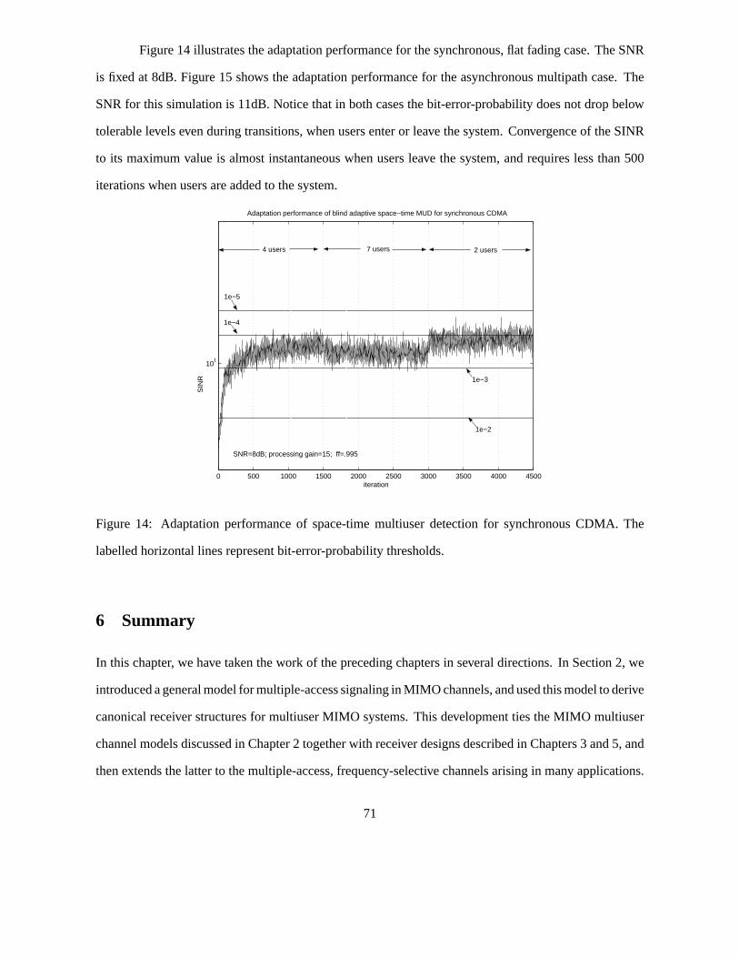
Figure 14 illustrates the adaptation performance for the synchronous, flat fading case. The SNR
is fixed at 8dB. Figure 15 shows the adaptation performance for the asynchronous multipath case. The
SNR for this simulation is 11dB. Notice that in both cases the bit-error-probability does not drop below
tolerable levels even during transitions, when users enter or leave the system. Convergence of the SINR
to its maximum value is almost instantaneous when users leave the system, and requires less than 500
iterations when users are added to the system.
0 500 1000 1500 2000 2500 3000 3500 4000 4500
101
Adaptation performance of blind adaptive space−time MUD for synchronous CDMA
SIN
R
iteration
1e−2
1e−3
1e−4
1e−5
4 users 7 users 2 users
SNR=8dB; processing gain=15; ff=.995
Figure 14: Adaptation performance of space-time multiuser detection for synchronous CDMA. The
labelled horizontal lines represent bit-error-probability thresholds.
6 Summary
In this chapter, we have taken the work of the preceding chapters in several directions. In Section 2, we
introduced a general model for multiple-access signaling in MIMO channels, and used this model to derive
canonical receiver structures for multiuser MIMO systems. This development ties the MIMO multiuser
channel models discussed in Chapter 2 together with receiver designs described in Chapters 3 and 5, and
then extends the latter to the multiple-access, frequency-selective channels arising in many applications.
71

0 500 1000 1500 2000 2500 3000 3500 4000 450010
0
101
Adaptation performance of blind adaptive space−time MUD for asynchronous multipath CDMA
SIN
R
iteration
1e−2
4 users 2 users
1e−3
1e−4
1e−5
SNR=11dB; processing gain=15; ff=.995
7 users
Figure 15: Adaptation performance of space-time multiuser detection for asynchronous multipath CDMA.
The labelled horizontal lines represent bit-error-probability thresholds.
Section 3 also echoes the detection problems discussed in Chapters 3 and 5,notably by re-emphasizing
the importance of iterative algorithms in complexity reduction for MIMO receivers. Section 4 describes
how the structure imposed by space-time coding techniques of Chapter 4 canbe exploited, together with
the turbo-style iterative methods of Chapter 5, can be used to significantly enhance the overall receiver
performance with little attendant increase in complexity. Although most of the work of the techniques in
this chapter apply to general interference-type channels (multi-access,inter-symbol, and inter-antenna),
the focus has been on the direct-sequence CDMA channels introduced inChapter 1. Section 5 specifically
deals with such channels, which are particularly amenable to adaptive implementation. Moreover, Section
5 exploits the Alamouti space-time coding structure described in Chapters 1 and 4 in its adaptation
algorithms.
72

7 Bibliographic Notes
As noted in Section 2, the methods discussed in this chapter have been developed over a period of several
decades. Early work on receiver design for channel-coded systemsand intersymbol-interference channels
dates from the 1960s and 1970s, respectively, while the techniques formultiple-access and inter-antenna
interference channels began largely in the 1980s and 1990s, respectively. A review of these developments
is found in [30]. Complexity reduction through iterative algorithms and through adaptation have been
major issues throughout this development, with turbo style algorithms gaining significant interest in the
1990s. (An overview of iterative techniques is found in [31].) The current decade has seen a number
of developments, particularly in the development of new analytical tools usingmethods of statistical
physics, and in refinement, analysis and understanding of adaptive anditerative methods. However, all
of these areas are still areas of active research, and new developments continue today. Perhaps the most
critical open issue lies in the transition of these methods into more widespread practice. Although current
wireless standards and systems do incorporate some of the ideas exposedin this chapter, there is still
considerable opportunity for further practical development. The iterative and adaptive methods are, of
course, directed at precisely this goal.
For further additional reading on the subject matter of this chapter, the reader is referred to the
books by Verdu [38], Wang and Poor [46], and Comaniciu, et al. [5]. The first of these three books
contains an excellent exposition of the fundamentals of multiuser detection, while the second contains
further elaboration and additional examples illustrating the model of Section 2,as well as considerable
discussion of various methods of adaptive and iterative receiver design. Issues not treated in this chapter,
such as fast fading and OFDM systems, are also considered there. Finally, the impact of these methods
on higher-layer networking issues, such as resource allocation, quality-of-service provision, and network
performance, is discussed in the third of these three books.
73
References
[1] S. M. Alamouti,A simple transmit diversity technique for wireless communications, IEEE Journ.
Select. Areas. Commun.16 (1998), no. 8, 1451 – 1458.
[2] L. R. Bahl, J. Cocke, F. Jelinek, and J. Raviv,Optimum decoding of linear codes for minimizing
symbol error rate, IEEE Trans. Inform. Theory20 (1974), no. 3, 284 – 287.
[3] C. Berrou and A. Glavieux,Near optimum error-correcting coding and decoding: Turbo codes,
IEEE Trans. Commun.44 (1996), no. 10, 1261 – 1271.
[4] C. Berrou, A. Glavieux, and P. Thitimajshima,Near Shanon limit error-correcting coding and
decoding: Turbo codes, Proc. 1993 Int. Conf. Commun. (Geneva, Switzerland), vol. 2, 1993,
pp. 1064–1070.
[5] C. Comaniciu, N. Mandayam, and H. V. Poor,Wireless networks: Multiuser detection in cross-layer
design., Springer, New York, NY, 2005.
[6] H. Dai, A. F. Molisch, and H. V. Poor,Downlink capacity of interference-limited mimo systems with
joint detection, IEEE Trans. Wireless Comm.3 (2004), no. 2, 442–453.
[7] H. Dai and H. V. Poor,Sample-by-sample adaptive space-time processing for multiuser detectionin
multipath CDMA systems, Proc. 2001 Fall IEEE Vehicular Technology Conference (Atlantic City,
NJ), Oct. 2001.
[8] , Iterative space-time processing for multiuser detection in multipath cdma channels, IEEE
Trans. Sig. Proc.50 (2002), no. 9, 2116–2127.
[9] M. O. Damen, A. Safavi, and K. Abed-Meriam,On CDMA with space-time codes over multipath
fading channels, IEEE Trans. Wireless Commun.2 (2003), 11–19.
[10] A. P. Dempster,Maximum likelihood from incomplete data via the EM algorithm, 1977, pp. 1–38.
[11] J. A. Fessler and A. O. Hero,Space-alternating generalized EM algorithm, IEEE Trans. Signal
Processing42 (1994), no. 10, 2664–2677.
74

[12] T. R. Giallorenzi and S. G. Wilson,Multiuser ML sequence estimator for convolutionally coded
asynchronous DS-CDMA systems, IEEE Trans. Commun.44 (1996), no. 8, 997–1008.
[13] , Suboptimum multiuser receivers for convolutionally coded asynchronousDS-CDMA sys-
tems, IEEE Trans. Commun.44 (1996), no. 9, 1183–1196.
[14] G. H. Golub and C. F. Van Loan,Matrix computation, The John Hopkins University Press, Baltimore,
MD, 1996.
[15] J.-C. Guey, M. P. Fitz, M. R. Bell, and W.-Y. Kuo,Signal design for transmitter diversity wireless
communication systems over Rayleigh fading channels, Proc. IEEE Veh. Technol. Conf. (Atlanta,
GA), 1996, pp. 136–140.
[16] A. R. Hammons and H. El Gamal,On the theory of space-time codes for PSK modulation, IEEE
Trans. Inform. Theory46 (2000), no. 2, 524 – 542.
[17] B. Hochwald, T. L. Marzetta, and C. B. Papadias,A novel space-time spreading scheme for wireless
CDMA systems, Proc.37th Ann. Allerton Conf. Commun., Contr., Comput. (Monticello, IL), Sep.
22-24, 1999.
[18] ,A transmitter diversity scheme for wideband CDMA systems based on space-time spreading,
IEEE Journ. Select. Areas. Commun.19 (2001), 48–60.
[19] J. Hou, J. E. Smee, H. D. Pfister, and S. Tomasin,Implementing interference cancellation to increase
the EV-DO REV A link capacity, IEEE Communications Magazine44 (2006), no. 2, 96–102.
[20] S. K. Jayaweera and H. V. Poor,Iterative multiuser detection for space-time coded synchronous
CDMA, Proc. IEEE Veh. Technol. Conf. (Atlantic City, NJ), vol. 4, Fall 2001,pp. 2736–2739.
[21] , Low complexity receiver structures for space-time coded multiple-accesssystems,
EURASIP Journ. Applied Signal Processing (Special Issue on Space-time Coding)2002 (2002),
275–288.
75
[22] P. Lancaster and M. Tismenetsky,The theory of matrices with applications, Academic Press, Inc.,
Orlando, FL, 1985.
[23] H. Li, X. Lu, and G. B. Giannakis,Capon multiuser receiver for CDMA systems with space-time
coding, IEEE Trans. Sig. Proc.50 (2002), 1193 – 1204.
[24] J. Liu, J. Li, H. Li, and E. G. Larsson,Differential space-time modulation for interference suppres-
sion, IEEE Trans. Sig. Proc.49 (2001), 1786–1795.
[25] Z. Liu, G. B. Giannakis, B. Muquet, and S. Zhou,Space-time coding for broadband wireless com-
munications, Wireless Syst. Mobile Comput.1 (2001), 35–53.
[26] B. Lu and X. Wang,Iterative receivers for multiuser space-time coding systems, IEEE Journ. Select.
Areas. Commun.18 (2000), no. 11, 2322 – 2335.
[27] A. Naguib and N. Seshadri,Combined interference cancellation and ML decoding of space-time
block codes, Proc. 7-th Commun. theory mini-conference at Globecom’98 (Sydney, Australia), 1998.
[28] I. Oppermann,CDMA space-time coding using an LMMSE receiver, Proc. Int. Conf. Commun.
(ICC’99) (Vancouver, BC, Canada), 1999, pp. 182–186.
[29] H. V. Poor,An introduction to signal detection and estimation, Springer-Verlag, New York, 1994.
[30] , Dynamic programming in digital communications: Viterbi decoding to turbo multiuser
detection, Journal of Optimization Theory and Applications115 (2002), no. 3, 629 – 657.
[31] , Iterative multiuser detection, IEEE Signal Processing Magazine21 (2004), no. 1, 81 – 88.
[32] H. V. Poor and S. Verdu, Probability of error in MMSE multiuser detection, IEEE Trans. Inform.
Theory (1997), 858–871.
[33] J. Proakis,Digital communications, fourth ed., McGraw-Hill, New York, 2000.
[34] D. Reynolds and X. Wang,Adaptive group-blind multiuser detection based on a new subspace
tracking algorithm, IEEE Trans. Commun.49 (2001), no. 7, 1135–1141.
76

[35] D. Reynolds, X. Wang, and H. V. Poor,Blind adaptive space-time multiuser detection with multiple
transmitter and receiver antennas, IEEE Trans. Signal Processing50 (2002), no. 6, 1261–1276.
[36] V. Tarokh, H. Jafarkhani, and A. R. Calderbank,Space-time block codes from orthogonal designs,
IEEE Trans. Inform. Theory45 (1999), no. 5, 1456 – 1467.
[37] V. Tarokh, N. Seshadri, and A. R. Calderbank,Space-time codes for high rate wireless communica-
tion: Performance criterion and code construction, IEEE Trans. Inform. Theory44 (1998), no. 2,
744 – 765.
[38] S. Verdu, Multiuser detection, Cambridge Univ. Press, Cambridge, UK, 1998.
[39] S. Verdu and H. V. Poor,Abstract dynamic programming models under commutativity conditions,
SIAM Journal on Control and Optimization25 (1987), no. 4, 990 – 1006.
[40] A. J. Viterbi, An intuitive justification and a simplified implementation of the MAP decoder for
convolutional codes, IEEE Journ. Select. Areas. Commun.16 (1998), no. 2, 260 – 264.
[41] X. Wang and A. Host-Madsen,Group-blind multiuser detection for uplink CDMA, IEEE Journ.
Select. Areas Commun.17 (1999), no. 11, 1971–1984.
[42] X. Wang and H. V. Poor,Blind equalization and multiuser detection for CDMA communications in
dispersive channels, IEEE Trans. Commun.COM-46 (1998), no. 1, 91–103.
[43] , Blind multiuser detection: A subspace approach, IEEE Trans. Inform. Theory44 (1998),
no. 2, 677–691.
[44] , Iterative (turbo) soft interference cancellation and decoding for coded CDMA, IEEE Trans.
Commun.47 (1999), no. 7, 1046 – 1061.
[45] , Space-time multiuser detection in multipath CDMA channels, IEEE Trans. Signal Process-
ing 47 (1999), no. 9, 2356–2374.
[46] , Wireless communication systems: Advanced techniques for signal reception, Prentice-Hall,
Upper Saddle River, NJ, 2002.
77
[47] Y. Zhang and R. S. Blum,Multistage multiuser detection for CDMA with space-time coding, Proc.
Tenth IEEE Workshop on Statistical Signal and Array Processing (Poconos, PA), Aug. 2000, pp. 1–5.
[48] R. E. Ziemer, R. L. Peterson, and D. E. Borth,Introduction to spread spectrum communications,
Prentice-Hall: Upper Saddle River, NJ, 1995.
78