multitaper power spectrum estimation - university of … · · 2016-01-11multitaper power...
TRANSCRIPT
Multitaper Power Spectrum Estimation Wim van Drongelen
Page | 1
Multitaper Power Spectrum Estimation
Wim van Drongelen, 2014
1. Introduction
The most commonly applied technique to obtain an estimated power spectrum )(ˆ fS of a sampled
time series )(tx of finite length N, is to compute the Fourier transform )2( fjX , followed by
multiplication by its complex conjugate and scaling by the length of the finite observation, i.e.
NfjXfjXfS /)2()2()(ˆ * (see Chapter 7 in van Drongelen, 2007). The reliability of this
estimated power spectrum is significantly reduced both by (1) the variance of the estimate )(ˆ fS
at each frequency f (i.e., the spectra usually look very noisy) and (2) by leakage of energy across
frequencies, creating a bias. The leakage is due to the fact that we take a finite section of signal,
which equates to multiplying the signal by a rectangular window (sometimes called a boxcar)
(see three upper traces in Fig. 1). The Fourier transform of the rectangular window shows
multiple side lobes (Fig. 2A) and this causes the leakage problem. Recall that multiplication in
the time domain is equivalent to a convolution in the frequency domain; hence there will be a
convolution of the signal transform and the boxcar’s Fourier transform resulting in leakage of
energy. A solution to reduce leakage in the frequency domain is to first multiply the signal in the
time domain with a (non-rectangular) window characterized by a Fourier transform with less
energy in its side lobes. The windowing approach described in this paragraph is explained in
more detail in van Drongelen (2007), Section 7.1.1. To summarize if we have a sequence )(tx of
length N, a window )(ta , the estimated spectrum is given by:
1
0
2
2)()()(ˆ
N
t
jftetatxfS . (1)
(Here and in the following, for convenience of comparison with Prieto et al. (2007), I adapt most
of their notation.)
If the window )(ta is not explicitly present in Equation (1), or if it is defined as a rectangular
window/boxcar, the spectral estimate )(ˆ fS is called the periodogram and it should be noted that
in this case, one may expect that bias due to leakage will be strong.
Of course, the use of a window (also called a taper) affects the estimate by reducing leakage but
it doesn’t change the variance of the estimate at each frequency. A common approach to reduce
the variance is taking an average across several frequencies and/or computing an average

Multitaper Power Spectrum Estimation Wim van Drongelen
Page | 2
spectrum from several time epochs. Averaging across frequencies reduces spectral resolution and
using multiple epochs is undesirable if the signal may be non-stationary.
Figure 1: Power spectrum of a finite observation
Example of a Gaussian white noise signal (zero mean and unit variance; upper trace) and a rectangular/boxcar
window (2nd
trace). When signal and window are multiplied, the result (depicted in the third trace) mimics a finite
observation of the signal with a length that is equal to the length of the rectangular window. The bottom trace shows
the periodogram of the finite observation. From the bottom graph it is obvious that the periodogram is very
noisy due to the variance in this estimate. The expected power is equal to the variance of the Gaussian distribution
from which the samples in the time domain signal are drawn (one in this example). Leakage of energy across
spectral bands, which is also present in this estimate (due to the applied boxcar window), cannot be directly
observed in this plot but can be deduced from the spectrum of the boxcar itself (e.g. see Fig. 7.4 in van Drongelen,
2007) when convolved with the signal in the frequency domain; see text and Section 7.1.1 in van Drongelen (2007)
for further explanation.
In Section 2, we will first introduce the use of multiple tapers and the rationale behind their
derivation. In Section 3, we depict an example of the application of this procedure by using a
Gaussian autoregressive process with a known power spectrum. From this example we conclude
that there is a need for optimization of the procedure, which is presented (without proof) in
Section 4. Finally, in Section 5, we show a concrete example of the optimized multitaper spectral
estimate in Matlab.
2. The Use of Tapers
The multitaper approach, first described in a seminal paper by Thomson (1982), improves the
spectral estimate by addressing both leakage and variance in the estimate. The basic approach is
simple: what is better than using a taper? … You guessed it … the answer is: you use multiple
tapers. In this approach, every taper kv out of a set of K tapers is a bit different and reduces
leakage of energy across frequencies. In addition, in Thomson’s approach, the tapers are

Multitaper Power Spectrum Estimation Wim van Drongelen
Page | 3
orthogonal and they are used to provide K orthogonal samples of the data )(tx . These samples are
used to create a set of K spectral estimates )(ˆ fSk that can be used to compute an average )( fS
with reduced variance:
K
k
k fSK
fS1
)(ˆ1)( . (2)
The general idea for the application of a taper is as follows. Each taper )(ta is associated with an
estimated spectrum that is given by equation (1). In order to maintain correct values for total
power, we assume the tapers are normalized such that 1)(
1
0
2
N
t
ta . Furthermore, the power
spectrum of taper )(ta is )(2
fA , and its spectral properties are important because they determine,
via convolution, the estimate of the power spectrum of our windowed (tapered) time series:
2/1
2/1
2
')'()'()( dfffSfAfS
. (3)
Note that we normalized the Nyquist frequency to ½. (Recall that multiplication in the time
domain is associated with convolution in the frequency domain; see Section 8.3.3 in van
Drongelen, 2007.)
A desirable taper will have low amplitude spectral values for all larger values of 'ff . In
other words, these tapers will have low energy in the side lobes. This leads to estimates for )( fS
that will mainly and correctly consist of values close to f . In this case, we will have minimal
leakage and thus bias in the spectral estimate.
The reasoning continues as follows. Suppose we want to estimate our spectrum with a resolution
bandwidth W, which is necessarily set at a value in between the resolution of the spectrum 1/N
and the maximum of the spectrum, the Nyquist frequency. To simplify notation, we assume that
the sample interval is unity and the Nyquist frequency is normalized at ½. The fraction of the
taper’s energy within the selected frequency band is given by:
2/1
2/1
2
2
)(
)(
),(
dffA
dffA
WN
W
W (4)
The basic idea is that we want to find the tapers with minimal leakage by maximizing , i.e. the
fraction of the energy within bandwidth W is maximized. To make a long story short (see
Appendix 1 for a longer story), one maximizes by setting the derivative of the expression in
Equation (4) with respect to vector )(ta equal to zero. This equates to solving the following, well
known matrix eigenvalue problem (see Appendix 1 for further details):
Multitaper Power Spectrum Estimation Wim van Drongelen
Page | 4
aaD , (5)
in which the N × N matrix D has components )'(
)'(2sin(',
tt
ttWD tt
. Note that this function has
even symmetry. Therefore D is a symmetric matrix. The solution has N eigenvalues (
110 ,...,,...,, Nk ) and orthonormal eigenvectors ( 110 ,...,,...,, Nk vvvv ) (recall that we normalize
them to unity: 1)(
1
0
2
N
tk tv ). The eigenvectors kv are so-called discrete prolate spheroidal
sequences, also called Slepian sequences (Slepian, 1978). (A prolate sphere is an elongated
spherical object with the polar axis greater than the equatorial diameter.)
Fig. 2
The spectrum of a rectangular window (boxcar) depicted in panel (A) has most energy concentrated in the desired
bandwidth indicated between the stippled vertical lines, but also shows a lot of energy in the side lobes. The function
in (B) is the spectrum of an ideal window where all energy is located within the interval between –w and w. When a
spectrum is convolved with the spectra of these windows, the one in (A) generates significant leakage and therefore
bias, whereas the ideal one in (B) gives a bias-free estimate. As shown in Figures 3 and 4, even the best optimized
window isn’t ideal as in panel (B), but definitely better than the one from the boxcar window depicted in panel (A).
Note that matrix D can be considered as the unscaled covariance matrix of the inverse transform
of a rectangular window between –W and W in the frequency domain (Fig. 2B, Appendix 1).
Therefore, the computation of eigenvalues and eigenvectors of D is the same as performing
principal component analysis (PCA) on the inverse transform of the ideal spectral window (see
van Drongelen (2010) for an introduction to PCA). Since the dimension of D is N × N, there are
N eigenvalues k and eigenvectors kv . The first set of components capture most of the properties
of this ideal window, whereas the subsequent components capture less, so the question is which
components to include when using them as tapers. The first eigenvalue is very close to one, so it
is associated with a very good eigenvector, i.e. a taper that minimizes leakage. Since we use the
discrete Fourier transform for obtaining the spectral estimate, the number of points P in
Multitaper Power Spectrum Estimation Wim van Drongelen
Page | 5
bandwidth W is a multiple of the spectral resolution 1/N of the sample time series: thus W = P/N
and P = NW. As shown in the table below, for choices of N = 128 and NW = 4, 3, or 2, the first
2NW-1 eigenvalues are all very close to unity (Table 1 from Park et al., 1987). Therefore, as a
first approach, the first 2NW-1 normalized eigenvectors could be considered good to use for
reducing leakage and also (by averaging their results) for reducing the variance of the spectral
estimate.
As you can imagine, there are a few alternatives for the average procedure of the tapered power
spectra. One might simply average as in Equation (2) above (which is what we will discuss in
Section 3), or one might improve the estimate by composing a weighted average (which gives
better results as you will see in Sections 4 and 5).
3. An Example
Let’s consider a concrete example of the use of the multitaper technique and analyze a signal that
is generated using an example of an AR process )(tx described by Percival and Walden (1993)
(their Equation (46a)):
)()4(9238.0)3(6535.2)2(8106.3)1(7607.2)( ttxtxtxtxtx (6)
Here )(t is a Gaussian White Noise (GWN) process with zero mean and unit variance. Since we
use this series to evaluate spectral analysis, we want to compute its power spectrum using the
approach described in Section 13.4 in van Drongelen (2007). If we z-transform the AR
expression: the transform of )(tx is )(zX , and since the transform of the GWN is 1)( zE , we get:
43214321 1
1
1
)()(
zdzczbzazdzczbza
zEzX
Multitaper Power Spectrum Estimation Wim van Drongelen
Page | 6
The Fourier transform )( jX can now be obtained by substitution tjez 1 and the power
spectrum by computing *XX . This theoretical power spectrum we will use as our gold standard
for comparison with our multitaper estimation.
The following is part of a Matlab routine that computes and plots the spectrum in (dB) versus
a frequency scale between 0 and 0.5 (as in Percival and Walden (1993) and in Figs. 3 and 4).
% constants of AR(4) in Eq (46a) in Percival and Walden, 1993 a=2.7607; b=-3.8106; c=2.6535; d=-.9238;
dt=1; % time step set to 1 w=0:.01:pi/dt; % scale for frequency f=w./(2*pi/dt); % frequency scaled between 0 and 0.5 (for plot) z=exp(-j*w*dt); % z^(-1)
X=1./(1-a*z-b*z.^2-c*z.^3-d*z.^4); % Fourier transform PX=X.*conj(X); % Power LPX=10*log10(PX); % Power in dB
figure;plot(f,LPX) % Compare theoretical spectrum Fig. 3 and 4 in Handout
The procedure we follow for this multitaper analysis is depicted in Figures 3 and 4 (plots from
Percival and Walden (1993), their Figs. 336 – 341). In this example we demonstrate that the
number of tapers used provides a compromise between reduction of leakage and variance. In this
example NW = 4 thus we would consider up to seven (2NW -1) eigenvectors. Figure 3 depicts
the properties of the individual tapers (the 8th
one is also shown), including their spectra and the
effects of their application in the time and frequency domains. In Figure 4, the effects of using
these tapers in spectral averages are shown. As can be seen in, the 1st and best taper reduces
leakage almost to zero (almost no energy in the side lobes) but produces a single spectral
estimate associated with rather large variance. Adding the result from a 2nd
taper adds a bit of
side lobes (and thus leakage) but averaging it with the 1st one reduces variance because now the
spectrum is averaged from two results. By including the result from each additional taper in the
averaged estimate, there is both a bit of increase of leakage and reduction of variability due to the
averaging procedure . In this example there seems to be a reasonable optimum at five tapers. At
eight tapers the window contains so much energy in the side lobes that it causes a large amount
of leakage and thus a strong bias in the spectral estimate. The take-home message of this
example is that including the results obtained with the first 2NW-1 tapers in the averaged spectral
estimate may still cause an unacceptable level of leakage! This problem will be further discussed
and addressed in Section 4 below.

Multitaper Power Spectrum Estimation Wim van Drongelen
Page | 7
Figure 3: Example of the properties of the individual tapers (NW = 4)
The left column in this set of plots shows eight discrete prolate spheroidal tapers. The 2NW, eight tapers (k = 1 - 8)
are depicted in subsequent rows. The panels in the 2nd
column are the products of the time series computed with
Equation (6) multiplied with these tapers. The 3rd
column shows the spectra of the tapers. The right column depicts
the estimate of the spectra of the windowed time series; the black line is the theoretical spectrum and the grey noisy
lines are the estimates of the windowed signals. Obviously the energy of the side lobes and the associated leakage
(especially in the range from 0.3 - 0.5) increases with k. This Figure is a combination of Figs. 336 – 339 in Percival
and Walden (1993).
Multitaper Power Spectrum Estimation Wim van Drongelen
Page | 8
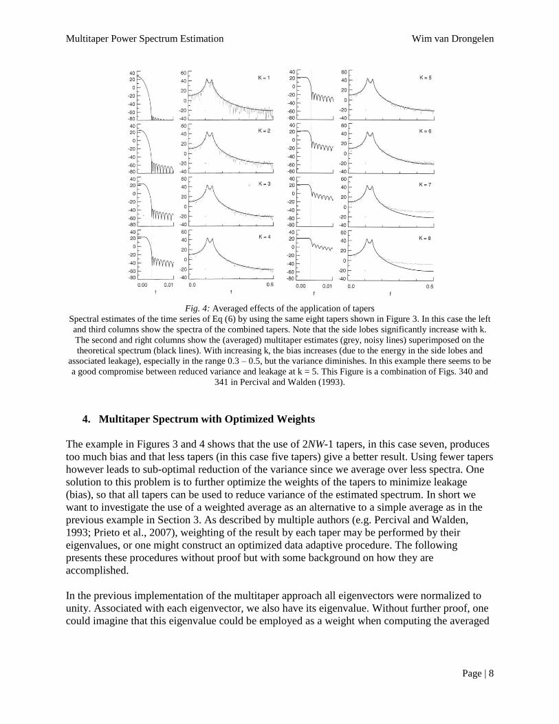
Fig. 4: Averaged effects of the application of tapers
Spectral estimates of the time series of Eq (6) by using the same eight tapers shown in Figure 3. In this case the left
and third columns show the spectra of the combined tapers. Note that the side lobes significantly increase with k.
The second and right columns show the (averaged) multitaper estimates (grey, noisy lines) superimposed on the
theoretical spectrum (black lines). With increasing k, the bias increases (due to the energy in the side lobes and
associated leakage), especially in the range 0.3 – 0.5, but the variance diminishes. In this example there seems to be
a good compromise between reduced variance and leakage at k = 5. This Figure is a combination of Figs. 340 and
341 in Percival and Walden (1993).
4. Multitaper Spectrum with Optimized Weights
The example in Figures 3 and 4 shows that the use of 2NW-1 tapers, in this case seven, produces
too much bias and that less tapers (in this case five tapers) give a better result. Using fewer tapers
however leads to sub-optimal reduction of the variance since we average over less spectra. One
solution to this problem is to further optimize the weights of the tapers to minimize leakage
(bias), so that all tapers can be used to reduce variance of the estimated spectrum. In short we
want to investigate the use of a weighted average as an alternative to a simple average as in the
previous example in Section 3. As described by multiple authors (e.g. Percival and Walden,
1993; Prieto et al., 2007), weighting of the result by each taper may be performed by their
eigenvalues, or one might construct an optimized data adaptive procedure. The following
presents these procedures without proof but with some background on how they are
accomplished.
In the previous implementation of the multitaper approach all eigenvectors were normalized to
unity. Associated with each eigenvector, we also have its eigenvalue. Without further proof, one
could imagine that this eigenvalue could be employed as a weight when computing the averaged

Multitaper Power Spectrum Estimation Wim van Drongelen
Page | 9
power spectrum estimate )( fS . Equation (2) is then modified by weighing the individual
contributions of each tapered estimate )(ˆ fSk by its associated eigenvalue k :
K
k k
k fS
KfS
1
)(ˆ1)(
(7)
As it appears, the approach of weighing the estimates by their eigenvalues may still not give the
best estimates. Using a regularization approach, Thompson (1982) developed a data adaptive
method to weigh the individual spectral estimates that contribute to the average. This leads to the
following expression for the spectral estimate:
K
k
k
K
k
kk
d
fSd
fS
1
2
1
2 )(ˆ
)( , (8a)
in which the weights kd are frequency dependent and computed by using:
2)1()(
)()(
kk
k
kfS
fSfd
, (8b)
with2 the variance of the time domain signal )(tx . However, the big unknown in the expression
for kd is the spectrum )( fS ! Often the first two eigenspectra )(ˆ fSk (for k = 0 and 1), provide an
initial estimate for )( fS and the adaptive weights are then found iteratively (for further details,
see Thompson, 1982; Percival and Walden, 1993).
5. An Example in Matlab
The approach to compute a multitaper estimate of the spectrum is implemented in the Matlab
pmtm command. In Matlab type: help pmtm to get the following description of the procedure.
pmtm Power Spectral Density (PSD) estimate via the Thomson multitaper
method (MTM).
Pxx = pmtm(X) returns the PSD of a discrete-time signal vector X in
the vector Pxx. Pxx is the distribution of power per unit frequency.
The frequency is expressed in units of radians/sample. pmtm uses a
default FFT length equal to the greater of 256 and the next power of
2 greater than the length of X. The FFT length determines the length
of Pxx.
For real signals, pmtm returns the one-sided PSD by default; for
complex signals, it returns the two-sided PSD. Note that a one-sided

Multitaper Power Spectrum Estimation Wim van Drongelen
Page | 10
PSD contains the total power of the input signal.
Pxx = pmtm(X,NW) specifies NW as the "time-bandwidth product" for the
discrete prolate spheroidal sequences (or Slepian sequences) used as
data windows. Typical choices for NW are 2, 5/2, 3, 7/2, or 4. If
empty or omitted, NW defaults to 4. By default, pmtm drops the last
taper because its corresponding eigenvalue is significantly smaller
than 1. Therefore, The number of tapers used to form Pxx is 2*NW-1.
Pxx = pmtm(X,NW,NFFT) specifies the FFT length used to calculate
the PSD estimates. For real X, Pxx has length (NFFT/2+1) if NFFT is
even, and (NFFT+1)/2 if NFFT is odd. For complex X, Pxx always has
length NFFT. If empty, NFFT defaults to the greater of 256
and the next power of 2 greater than the length of X.
[Pxx,W] = pmtm(...) returns the vector of normalized angular
frequencies, W, at which the PSD is estimated. W has units of
radians/sample. For real signals, W spans the interval [0,Pi] when
NFFT is even and [0,Pi) when NFFT is odd. For complex signals, W
always spans the interval [0,2*Pi).
[Pxx,W] = pmtm(X,NW,W) where W is a vector of normalized
frequencies (with 2 or more elements) computes the PSD at
those frequencies using the Goertzel algorithm. In this case a two
sided PSD is returned. The specified frequencies in W are rounded to
the nearest DFT bin commensurate with the signal's resolution.
[Pxx,F] = pmtm(...,Fs) specifies a sampling frequency Fs in Hz and
returns the power spectral density in units of power per Hz. F is a
vector of frequencies, in Hz, at which the PSD is estimated. For real
signals, F spans the interval [0,Fs/2] when NFFT is even and [0,Fs/2)
when NFFT is odd. For complex signals, F always spans the interval
[0,Fs). If Fs is empty, [], the sampling frequency defaults to 1 Hz.
[Pxx,F] = pmtm(X,NW,F,Fs) where F is a vector of
frequencies in Hz (with 2 or more elements) computes the PSD at
those frequencies using the Goertzel algorithm. In this case a two
sided PSD is returned. The specified frequencies in F are rounded to
the nearest DFT bin commensurate with the signal's resolution.
[Pxx,F] = pmtm(...,Fs,method) uses the algorithm specified in method
for combining the individual spectral estimates:
'adapt' - Thomson's adaptive non-linear combination (default).
'unity' - linear combination with unity weights.
'eigen' - linear combination with eigenvalue weights.

Multitaper Power Spectrum Estimation Wim van Drongelen
Page | 11
[Pxx,Pxxc,F] = pmtm(...,Fs,method) returns the 95% confidence interval
Pxxc for Pxx.
[Pxx,Pxxc,F] = pmtm(...,Fs,method,P) where P is a scalar between 0 and
1, returns the P*100% confidence interval for Pxx. Confidence
intervals are computed using a chi-squared approach. Pxxc(:,1) is the
lower bound of the confidence interval, Pxxc(:,2) is the upper bound.
If left empty or omitted, P defaults to .95.
[Pxx,Pxxc,F] = pmtm(X,E,V,NFFT,Fs,method,P) is the PSD estimate,
confidence interval, and frequency vector from the data tapers in E and
their concentrations V. Type HELP DPSS for a description of the matrix
E and the vector V. By default, pmtm drops the last eigenvector because
its corresponding eigenvalue is significantly smaller than 1.
[Pxx,Pxxc,F] = pmtm(X,DPSS_PARAMS,NFFT,Fs,method,P) uses the cell
array DPSS_PARAMS containing the input arguments to DPSS (listed in
order, but excluding the first argument) to compute the data tapers.
For example, pmtm(x,{3.5,'trace'},512,1000) calculates the prolate
spheroidal sequences for NW=3.5, NFFT=512, and Fs=1000, and displays
the method that DPSS uses for this calculation. Type HELP DPSS for
other options.
[...] = pmtm(...,'DropLastTaper',DROPFLAG) specifies whether pmtm
should drop the last taper/eigenvector during the calculation. DROPFLAG
can be one of the following values: [ {true} | false ].
true - the last taper/eigenvector is dropped
false - the last taper/eigenvector is preserved
[...] = pmtm(...,'twosided') returns a two-sided PSD of a real signal
X. In this case, Pxx will have length NFFT and will be computed over
the interval [0,2*Pi) if Fs is not specified and over the interval
[0,Fs) if Fs is specified. Alternatively, the string 'twosided' can be
replaced with the string 'onesided' for a real signal X. This would
result in the default behavior.
The string input arguments may be placed in any position in the input
argument list after the second input argument, unless E and V are
specified, in which case the strings may be placed in any position
after the third input argument.
pmtm(...) with no output arguments plots the PSD in the current figure
window, with confidence intervals.
EXAMPLE:
Fs = 1000; t = 0:1/Fs:.3;

Multitaper Power Spectrum Estimation Wim van Drongelen
Page | 12
x = cos(2*pi*t*200)+randn(size(t)); % A cosine of 200Hz plus noise
pmtm(x,3.5,[],Fs); % Uses the default NFFT.
Figure 5 depicts how the multitaper computation (using the default data adaptive method)
applied to the AR(4) time series work in Matlab, and how its result compares to the standard
periodogram.
Figure 5: Comparison of the multitaper and boxcar methods
Comparison of the theoretical spectrum of the AR(4) time series and the periodogram and the multitaper spectrum
using the pmtm command. Note that the multitaper spectrum, as compared to the periodogram, has less bias across
the whole bandwidth. The variance at the lower frequencies is also less in the multitaper spectrum but not so much
at the higher frequencies in this example. This Figure was made with Matlab script ARspectrum.m. Note that if you
use this Matlab script (listed below), results can vary due to the random generation of the time series!
The results in Figure 5 were obtained with the following Matlab script ARspectrum.m % ARspectrum.m
clear; close all;
% constants of AR(4) in Eq (46a) in Percival and Walden, 1993 a=2.7607; b=-3.8106; c=2.6535; d=-.9238;
dt=1; % time step set to 1 w=0:.001:pi/dt; % scale for frequency f=w./(2*pi/dt); % frequency scaled between 0 and 0.5 (for plot) z=exp(-j*w*dt); % z^(-1)
X=1./(1-a*z-b*z.^2-c*z.^3-d*z.^4); % Fourier transform PX=X.*conj(X); % Power LPX=10*log10(PX); % Power in dB
figure;plot(f,LPX) % Compare theoretical spectrum Figs. 3 and 4 in Handout title('Spectrum AR(4)'); xlabel('Frequency'); ylabel('Power (dB)');
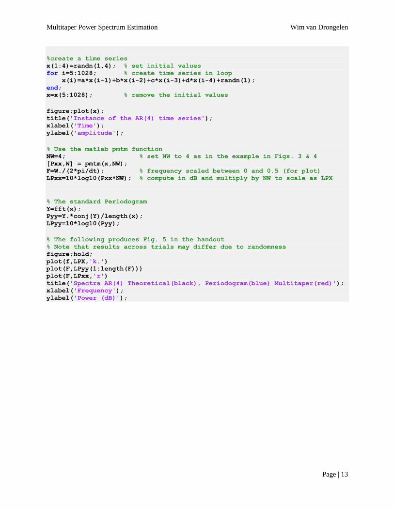
Multitaper Power Spectrum Estimation Wim van Drongelen
Page | 13
%create a time series x(1:4)=randn(1,4); % set initial values for i=5:1028; % create time series in loop x(i)=a*x(i-1)+b*x(i-2)+c*x(i-3)+d*x(i-4)+randn(1); end; x=x(5:1028); % remove the initial values
figure;plot(x); title('Instance of the AR(4) time series'); xlabel('Time'); ylabel('amplitude');
% Use the matlab pmtm function NW=4; % set NW to 4 as in the example in Figs. 3 & 4 [Pxx,W] = pmtm(x,NW); F=W./(2*pi/dt); % frequency scaled between 0 and 0.5 (for plot) LPxx=10*log10(Pxx*NW); % compute in dB and multiply by NW to scale as LPX
% The standard Periodogram Y=fft(x); Pyy=Y.*conj(Y)/length(x); LPyy=10*log10(Pyy);
% The following produces Fig. 5 in the handout % Note that results across trials may differ due to randomness figure;hold; plot(f,LPX,'k.') plot(F,LPyy(1:length(F))) plot(F,LPxx,'r') title('Spectra AR(4) Theoretical(black), Periodogram(blue) Multitaper(red)'); xlabel('Frequency'); ylabel('Power (dB)');

Multitaper Power Spectrum Estimation Wim van Drongelen
Page | 14
Appendix 1
Here we elaborate on the steps between Equations (4) and (5). For further details, see also
Percival and Walden (1993), p. 104 etc.
For convenience we repeat equation (4):
2/1
2/1
2
2
)(
)(
),(
dffA
dffA
WN
W
W . (4)
We need to maximize this expression for . First we limit the signal in the time domain over the
interval ]1,0[ N so that we can use the following expression for the discrete Fourier transform:
1
0
2)()(
N
t
jftetafA
.
Using Parseval’s theorem, we can rewrite the denominator in Equation (4) as:
1
0
2)(N
t
ta . (A1-1)
The numerator in Equation (4) can also be written as (note the use of dummy variables t and t’
and complex conjugate signs, *):
W
W
N
t
W
W
N
t
W
W
W
W
dfjft
etadfjft
etadffAdffA1
0'
1
0
** '2)'(
2)()()(
Now we change the order of summation and integration and combine the integrals over f:
)'()'(2
)('2
)'(2
)(
)'(2
)'(2
1
*1
0'
1
0
1
0'
1
0
* tadfttj
etadfjft
etadfjft
eta
W
W
ttjfettj
W
W
N
t
N
t
N
t
W
W
N
t
W
W
(A1-2)

Multitaper Power Spectrum Estimation Wim van Drongelen
Page | 15
Note that in the above expression, each of the two integrals left of the equal sign is the inverse
Fourier transform of a rectangular window in the frequency domain (this window ranges from
-W to W, e.g. Fig. 2B). The resulting integral in Equation (A1-2) generates the covariance of this
rectangular window:
)'(
)'(2sin
)'(2
1
)'(2
1
)'(2sin2
)'(2)'(2)'(2
tt
ttWee
ttje
ttjttWj
ttjWttjW
W
W
ttjf
(A1-3)
Combining Equations (A1-1) – (A1-3) to rewrite Equation (4), we get:
1
0
2
*1
0'
1
0
)(
)'()'(
)'(2sin)(
),(N
t
N
t
N
t
ta
tatt
ttWta
WN
This can be compactly rewritten in matrix/vector notation as:
aa
aDa
. (A1-4)
Here we simplified notation for and a, while matrix D is given by:
)'(
)'(2sin)',(
tt
ttWttD
. (A1-5)
In order to reduce leakage we need to maximize the expression for in Equation (A1-4). We
accomplish this by setting the derivative of this expression with respect to a equal to zero. If we
simplify Equation (A1-4) to the fraction u/v, the expression to solve is 0/)''( 2 vuvvu , which
is the same as solving 0'' uvvu . This can be rewritten as vuvu /'/' , or 0'' vu . Now
we recall from Equation (A1-4) that aDau and that thus aDu 2' . Note that this is the
case because matrix D is symmetric and not a function of a. The denominator aav , and its
derivative av 2' . Now we combine the expression for 'u and 'v with 0'' vu , we divide by 2
and we get Equation (5), the well-known eigenvalue expression:
0 aaD or aaD (5)

Multitaper Power Spectrum Estimation Wim van Drongelen
Page | 16
References
Park J, Lindberg CR and Vernon FL (1987) Multitaper spectral analysis of high-frequency
seismograms. J. Geophys. Res. 92: 12,675-12,684.
Percival DB and Walden AT (1993) Spectral Analysis for Physical Applications: Multitaper and
Conventional Univariate Techniques. Cambridge University Press, Cambridge, UK.
Prieto GA, Parker RL, Thomson DJ, Vernon FL and Graham RL (2007) Reducing the bias of
multitaper spectrum estimates. Geophys. J. Int. 171: 1269-1281.
Slepian D (1978) Prolate spheroidal wave functions, Fourier analysis, and uncertainty V: the
discrete case. Bell System Tech. J. 57: 1371-1429.
Thomson DJ (1982) Spectrum estimation and harmonic analysis. Proc. IEEE 70: 1055-1096.
Van Drongelen W (2007) Signal Processing for Neuroscientists: An Introduction to the Analysis
of Physiological Signals. Academic Press, Elsevier, Amsterdam.
Van Drongelen W (2010) Signal Processing for Neuroscientists: A Companion Volume.
Advanced Topics, Nonlinear Techniques and Multi-Channel Analysis. Elsevier, Amsterdam.
Homework
1. Modify the ARspectrum.m script to investigate the effect of the ‘adapt’, ‘unity’, and
‘eigen’ options in the pmtm command. What do these options mean and what can you
conclude?
2. What is the variance of the averaged spectral estimate )( fS if we have K spectral
estimates )( fSk
each with a variance of 2 (Using Equation (2))?