Multiscale Modeling of Fatigue for Ductile Materials

Caglar Oskay and Jacob FishCivil and Environmental Engineering Department

Rensselaer Polytechnic Institute, Troy, NY, 12180, USA

Abstract

A multiscale model is developed for fatigue life predictions of elastoplastic solids andstructures. The fatigue problem is formulated using a variant of the mathematical homoge-nization theory developed to account for almost periodic fields. Multiple temporal scales areemployed to resolve the solution within a load cycle as well as to predict the useful life spanof a structural component. The concept of almost-periodicity is introduced to account for ir-reversible inelastic deformation, which gives rise to nonperiodic fields in time domain. Bythis approach the original initial boundary value problem is decomposed into coupled micro-chronological (fast time-scale) and macro-chronological (slow time-scale) problems. The pro-posed life prediction methodology was implemented in ABAQUS and verified against the di-rect cycle-by-cycle simulation.

Keywords:temporal homogenization, almost periodicity, fatigue life prediction, multiscale mod-eling, ductile crack growth.

1 Introduction

The phenomenon of fatigue inherently involves multiple temporal and spatial scales. Multipletemporal scales exist due to the disparity between the period of a single load cycle acting on astructural component, which may be in the order of seconds, and the overall design life, whichmay span years. Likewise, multiple spatial scales exist due to the presence of micro- size cracksor inclusions with respect to the large size of the component of interest. Given this tremendousdisparity of spatial and temporal scales, life predictions pose a great challenge to mechanics andmaterials communities.

While fatigue life prediction methods range from experimentation to modeling, the primarydesign tool today is experimental, based on so-called S-N (in case of high cycle fatigue) andε-N (incase of low cycle fatigue) curves, which relate the component life to cyclic stress or strain. Fatigueexperiments are generally limited to specimens or small structural components, and therefore,boundary and initial conditions between the interconnect and the remaining structure requires somesort of modeling.

Paris’s law [1] represents one of the first attempts to empirically model fatigue life. It statesthat under ideal conditions of high cycle fatigue (or small scale yielding) and constant amplitude

1

loading, the growth rate of long cracks depends on the amplitude of the stress intensity factors (forvarious variants, see [2, 3, 4, 5, 6]). Obviously, these ideal conditions do not exist in practice. Evenunder ideal cyclic loading conditions, the crack tip does not experience cyclic stress amplitude dueto changing fracture mode caused by crack propagation and interaction between cracks.

Temporal scales can be resolved by means of cycle-by-cycle simulation, which has been re-cently reported (e.g., [7, 8]) in conjunction with cohesive zone models. Cycle-by-cycle simulation,however, may not be feasible for large systems undergoing large number of cycles. A so-called”cycle jump” technique [9, 10, 11] can be used to bridge the time scales. Although this approachhas been shown to be effective to simulate the evolution of state variables, the governing equationsare not guaranteed to be satisfied.

In this manuscript, a multiscale fatigue life prediction methodology is developed for both, theductile and brittle materials. The proposed methodology is based on the generalization of themathematical homogenization theory to account for non-periodicity in time domain. The non-periodicity is a byproduct of irreversible processes, such as damage accumulation, which naturallyviolates the condition of temporal periodicity. In this manuscript, the non-periodic contribution ismodeled as an orderζ¿ 1 perturbation to the periodic field. Since the periodic fields are assumedto be of order one and the nonperiodic contribution of orderζ ¿ 1 the resulting formulation iscoined as the temporal homogenization for almost periodic fields. The theory presented here differsfrom the classical mathematical homogenization in two respects:

1. In contrast to the classical (spatial or temporal) homogenization theory, the local fields areallowed to deviate from the condition of local periodicity. The almost periodicity means thatat the neighboring points homologous by periodicity, the value of a response function mayhave a variation of orderζ¿ 1.

2. A two-term order one (macro- and micro-chronological) expansion is used to approximatethe displacement field. This is in contrast to the classical homogenization where the micro-chronological contribution is of orderζ (and thus giving rise to order one contribution in thederivatives). In a typical fatigue problem both the oscillatory field and the nonperiodic fieldresulting for example from the dead or live load could be of the same order and thus thecorresponding displacements should be of the same order as well.

The present manuscript builds on the previous work of the authors [12] on high-cycle fatiguelife predictions for brittle materials where the response fields were modeled as locally periodic(τ-periodicity) whereas the state variables (i.e., state of damage) were assumed to be almost-τ-periodic. In the low-cycle fatigue considered in the present manuscript, all fields are modeled asalmost periodic.

Nonperiodic fields were considered in a number of other engineering applications, particularlyfor the analysis of composite media with randomly distributed inclusions using stochastic [13,14, 15, 16] and deterministic approaches [17, 18, 19, 20, 21], as well as for graded and stratifiedcomposites [22]. From the mathematical perspective, non-periodicity and almost periodicity withthe associated convergence relations have been investigated and reported in a number of articlesand monographs mainly in the field of spatial homogenization [23, 24, 25, 26, 27].

The multiscale fatigue model is developed for the case of accumulation of damage (microvoids)in the presence of elastoplastic effects, and propagation of macrocracks up to failure. Distributeddamage is modeled using a modified Gurson’s (GTN) model [28]. Damage accumulation is char-acterized by the nucleation, growth and coalescence of microvoids [28]. Kinematic hardening and

2

irreversible damage are incorporated into the model to generate a hysteretic behavior and to pre-vent shakedown and premature crack arrest. The propagation of cracks is simulated by the voidgrowth and coalescence which is a precursor to strain softening, and loss of ellipticity resultingin mesh sensitivity. A number localization limiters are known (e.g., [29, 30, 31, 32, 33]), but thisissue is not addressed in the present paper.

The remaining of this manuscript is organized as follows. Section 2 addresses the fundamentalaspects of the temporal homogenization in the presence of almost periodic fields. The problemstatement for the fatigue life prediction analysis of ductile solids based on the GTN model is givenin Section 3. Section 4 presents the formulation of the proposed multiscale methodology. Section 5focuses on computational issues. Verification studies are given in Section 6. In Section 7, futureresearch directions are discussed.

2 Multiple temporal scales with almost periodic functions

Multiple temporal scales are introduced to model slow degradation of material properties due tofatigue loading and the resulting crack propagation, as well as to resolve the deformation within asingle load cycle. Amacro-chronologicalscale, denoted by the intrinsic time coordinate,t, and amicro-chronologicalscale, denoted by the fast time coordinate,τ, are introduced. These two scalesare related through a small positive scaling parameter,ζ:

τ =tζ

; 0 < ζ¿ 1 (1)

where, the scaling parameter,ζ, is defined by the ratio:

ζ =τo

tr(2)

in which, tr andτo are the characteristic lengths of the macro- and the micro-chronological scales,respectively. The response fields, denoted byφ, are assumed to depend on the multiple temporalscales:

φζ(x, t) = φ(x, t,τ(t)) (3)

where, superposedζ denotes a rapidly oscillating function in time; andx is the spatial coordinates.Time differentiation in the presence of multiple temporal scales directly follows from the chainrule:

φζ(x, t) = φ(x, t,τ) = φ,t(x, t,τ)+1ζ

φ,τ(x, t,τ) (4)

in which, the comma followed by a subscript coordinate denotes partial derivative; and superposeddot is a total time derivative.

In the classical (spatial) homogenization theory [34], the response fields are commonly con-sidered to be locally periodic. Local periodicity implies that at the neighboring points in themacro-domain, homologous by periodicity, the value of a response function is the same, but atdifferent points in the macro-domain, the value of the function can be different. In the temporalhomogenization analysis of structures under fatigue loads, the state of the structure or componentis characterized by the accumulation of damage, which is generally irreversible in nature due tothermodynamic effects. Therefore, the associated response fields cannot be modeled using the

3

classical framework of local periodicity. Instead, we introduce the concept ofalmost periodicitytostudy fatigue response of ductile materials. The almost periodicity implies that, at the neighboringpoints in a spatial or temporal domain homologous by periodicity, the change in the value of aresponse function could be of orderζ. Figure 1 depicts an example of the almost periodic functionin time domain.

The basic properties of the almost periodic functions are subsequently discussed. We define aspace,T , consisting of all response functions, which can be represented in the form:

φap(x, t,τ) = φp(x, t,τ)+ζτφ(x) (5)

Theκ-periodic function,φp(x, t,τ), has the following property:

φp(x, t,τ+kκ)−φp(x, t,τ) = 0; k∈ N (6)

Settingφζp(x, t) = φp(x, t, t/ζ), the following relation exist [35]:

limζ→0

∫

Tζφζ

p(x, t)dt→∫

T

⟨φp(x, t,τ)

⟩dt (7)

for any closedT ∈ R. The periodic temporal homogenization (PTH) operator,〈·〉, is defined as:

〈·〉=1|κ|

∫

κ(·)dτ (8)

It is important to note that the almost periodic function,φap does not satisfy (7):

limζ→0

∫

Tζφζ

apdt = limζ→0

∫

Tζφζ

pdt+ φt2

2

∣∣∣∣T

(9a)

∫

T

(1|κ|

∫

κφapdτ

)dt =

∫

T

⟨φp

⟩dt+

ζ2

φ|κ| τ2

∣∣κ t|T (9b)

or in other words, in the asymptotic limitφap does not weakly converge to⟨φap

⟩.

This serves as a motivation to defining the almost periodic temporal homogenization (APTH)operator, denoted asM(φ):

M(φ),t (x, t) =⟨φ⟩(x, t) (10)

so that the weak convergence statement (7) can be extended to almost periodic functions inT , i.e.,

limζ→0

∫

Tζφζ

apdt→∫

TM(φap(x, t,τ))dt (11)

where,φζap(x, t) = φap(x, t, t/ζ). Substituting (5) into the right hand side, and using (7), it can be

easily seen that relation (11) is satisfied for allφap∈ T :∫

TM(φap)dt =

∫

T

(∫ [1ζ

⟨φap,τ

⟩+

⟨φap

⟩,t

]dt

)dt =

∫

T

(∫ [φ+

⟨φp

⟩,t

]dt

)dt

=∫

T

(tφ+

⟨φp

⟩)=

∫

Tφpdt+ φ

t2

2

∣∣∣∣T

(12)

Figure 2 depicts an example of the almost periodic fields. It compares the classical averagingoperator,〈φ〉 defined by Eq. 8 with an average function for almost periodic field,M(φ), definedby the APTH operator in 10. It can be clearly seen that〈φ〉 fails to track the average response ofthe almost periodic function, whereas the APTH operator does precisely that. Further discussionfollows in Section 4.

4

Figure 1: A locally almost periodic response field in time.

φ (x,t)ζ

φ (x,t)

φ (x,t)ζ

M(φ)(x,t)D E

φ D E

φ −ζ

φ −ζ M(φ)

Figure 2: Decomposition of the response fields with respect to periodic and almost periodic tem-poral homogenization operators.

5

3 Problem statement

Progressive damage of elastoplastic materials caused by void nucleation and growth is commonlyidealized using Gurson’s model [36]. Gurson’s model is a phenomenological model of combineddamage and plasticity formulated based on limit analysis of a hollow spherical void embeddedin the Von-Mises matrix material. A number of studies have been conducted over the years toassess the micro-mechanical and localization characteristics [37, 38] of the original model [36], andmodifications have been proposed to improve its predictions by incorporating void nucleation [39]and coalescence [40], hardening characteristics [41, 42], void shape effects [43] and others. Thestate-of-the-art today is the so-called Gurson-Tvergaard-Needlemen (GTN) model, which has beenvalidated for predicting the response of porous ductile materials under monotonic [44] as well asfor cyclic [45, 46] loading conditions.

The initial boundary value problem for the damage process of ductile materials using the GTNmodel may be written as:

Equilibrium equation: ∇ ·σσσζ + bζ = 0 on Ω× (0, to) (13)

Constitutive equation: σσσζ = L :(εεεζ− µµµζ

)on Ω× (0, to) (14)

Kinematic equation: εεεζ =12

(∇uζ +uζ∇) on Ω× (0, to) (15)

Initial condition: uζ = u′ on Ω (16)

Boundary conditions: uζ = uζ on Γu× (0, to) (17)

nσσσζ = tζ on Γt × (0, to) (18)

with the usual assumption of additive split:

εεεζ = eζ +µµµζ (19)

where,uζ is the displacement vector;σσσζ is the Cauchy stress tensor;εεεζ, eζ, and,µµµζ, are the total,elastic and plastic strain tensors, respectively;L is the tensor of elastic moduli;∇ is the vectordifferential operator given by∇ = (∂/∂x1, ∂/∂x2, ∂/∂x3) in Cartesian coordinate system;bζ is thebody force;Ω andΓ are the spatial problem domain and its boundary, respectively;u′ is the initialdisplacement field;uζ andtζ are the prescribed displacements and tractions on the boundariesΓu

andΓt , respectively, whereΓ = Γu∪Γt andΓu∩Γt = /0. For simplicity, analysis is restricted tosmall deformations.

The yield function of the GTN model with mixed hardening is expressed as:

Φζ ≡Φζ (σσσζ,Hζ) =(qζ)2

(σζ

F

)2 +2q1 f ζ cosh

(−3

2q2

pζ

σζF

)−1− (

q1 f ζ)2 = 0 (20)

where,H denotes the set of internal state variables;q1 andq2 are the Tvergaard constants;

qζ =

√32

sζ : sζ, sζ = ΘΘΘζ + pζδδδ, ΘΘΘζ = σσσζ−αααζ, pζ =−13

ΘΘΘζ : δδδ (21)

where,αααζ is the center of the yield surface; andδδδ is the second order identity tensor. The radius ofthe yield surface of the matrix material,σζ

F , is defined as [41]:

σζF = (1−b)σy +bσζ

M (22)

6

where,σy and σζM are the initial yield and matrix flow stresses, respectively; andb ∈ [0,1] is

a constant.b = 1, b = 0, andb ∈]0,1[ correspond to the pure isotropic, kinematic, and mixedhardening conditions, respectively.

The void coalescence function,f ζ( f ζ), is introduced to predict the loss of material stress car-rying capacity at a realistic state of void volume fraction. Following Tvergaard [40], the voidcoalescence is modeled using the piecewise linear function:

f ζ =

f ζ f ζ < fc

fc +(

1q1− fc

)f ζ− fcf f − fc

f ζ ≥ fc(23)

in which, critical void volume fraction,fc, and void volume fraction at failure,f f , are materialparameters. Whenf ζ approachesf f , f ζ → 1/q1, and the material looses its stress carrying capacity.

At a material point, the void volume fraction is allowed to grow due to the nucleation of new,as well as the growth of existing voids. The evolution equation of the void volume fraction may bethen written as:

f ζ = f ζgrowth+ f ζ

nucleation (24)

The rate of growth of the void volume fraction is non-zero only after the onset of plastic yieldingunder tensile loading:

f ζgrowth = (1− f ζ)〈µµµζ : δδδ〉+ (25)

where,〈·〉+ = [(·)+ | · |]/2 are MacCauley brackets. MacCauley brackets are introduced to avoidclosure of voids under compressive stress, which may otherwise prevent damage accumulationin some loading conditions, such as when the material experiences yielding in both tension andcompression within a single load cycle. In this study, a plastic strain controlled void nucleation isadopted [39]:

f ζnucleation= A ζ (ρζ) ρζ (26)

where,A ζ is taken to have a normal distribution:

A ζ (ρζ) =fN

sN√

2πexp

−1

2

(ρζ− εN

sN

)2

if ρζ > 0, µµµζ : δδδ > 0 (27)

in which, ρζ is the equivalent plastic strain; material parameter,fN, is the volume fraction ofvoid nucleating particles;εN is the mean strain for nucleation; andsN is the standard deviation ofnucleation.

The rate of the effective plastic strain is formulated based on the postulate that the rate of plasticwork of the matrix material is equivalent to the plastic work rate of the entire unit cell:

ρζ =ΘΘΘζ : µµµζ

(1− f ζ)σζF

(28)

The equivalent plastic strain rate is related to the matrix flow strength using the following equation:

σζM =

(EEt

E−Et

)ρζ = Et ρζ (29)

7

in which E is the Young’s modulus; andEt is the tangent to the uniaxial true stress- natural straindiagram at a given stress level. The uniaxial stress-strain diagram at a given stress level.

The plastic part of the strain rate is chosen to follow the normality rule:

µµµζ = λζ ∂Φζ

∂σσσζ; λζ ≥ 0 (30)

in which, λζ is the consistency parameter. The evolution equation for the yield surface motion isexpressed using Ziegler’s hardening rule:

αααζ = ϑζΘΘΘζ; ϑζ ≥ 0 (31)

The consistency parameters,λζ andϑζ are evaluated by employing the usual complementary andconsistency conditions.

4 Multiple temporal scale analysis

We start by expanding the response fields using the dual decomposition:

φ(x, t,τ) = φo(x, t)+φ1(x, t,τ) (32a)

= M(φ)(x, t)+ φ(x, t,τ) (32b)

in which, φ denotes the response fields (displacement, strain, stress) or internal state variables.Equation (32) is defined such that: ⟨

φ1(x, t,τ)⟩

= 0 (33)

Employing the definition of the APTH operator given by (10), and dual decompositions (32), thefollowing relations can be inferred:

φ,τ = φ1,τ,

⟨φ⟩,t =−1

ζ⟨φ,τ

⟩, φ = φ1−M

(φ1) , M(φo) = φo (34)

In view of the above definitions, the original boundary value problem is sought to be decom-posed into coupled macro-chronological (homogenized) and micro-chronological (cell) boundaryvalue problems. In what follows, the decompositions of the kinematic conditions, equilibriumequations, constitutive relations, and initial and boundary conditions are presented.

The strain tensor may be decomposed by applying (32) to the displacement field, substitutingthe resulting fields into (15), and exploiting the linearity of the PTH and APTH operators:

εεεm =12

(∇um+um∇) ; m= 0,1 (35)

M(εεε) =12

(∇M(u)+M(u)∇) , εεε =12

(∇u+ u∇) (36)

Applying (32a) to the stress, strain, and the plastic strain fields, substituting the resulting equa-tions into the elastoplastic constitutive equation, exploiting the dual decomposition relation (34a),and gathering the terms of the same order yields:

O(ζ−1) : σσσ,τ = L :

(εεε,τ− µµµ,τ

)on Ω× (0,τo) (37a)

O(1) : σσσo,t +σσσ1

,t = L :(εεεo,t + εεε1

,t −µµµo,t −µµµ1

,t

)(37b)

8

The constitutive equation for the micro-chronological problem is given by (37a). The macro-chronological constitutive relation is obtained by applying the PTH operator to (37), employ-ing (33), and exploiting the definition of the APTH operator:

M(σσσ),t = L :(M(εεε),t −M(µµµ),t

)= L :

[1ζ

(〈εεε,τ〉−⟨µµµ,τ

⟩)+ εεεo

,t −µµµo,t

]on Ω× (0, to) (38)

Next, we formulate the evolution equations for the micro- and macro-chronological problems.The consistency parameter of the flow rule,λ, is evaluated using the consistency condition whichinvolves rate relations (i.e.,Φ = 0). At a specified material point,x, the following two-scaleexpansion is employed:

λ(t,τ) =1ζ

λ1(t,τ)+λo(t) (39)

in which, λ1 and λo may be interpreted as consistency parameters induced by the micro- andmacro-chronological loadings, respectively. The yield condition may be expressed in terms of themicro- and macro-chronological fields:

Φ(t,τ)≡Φ(σσσ,H) = Φ(M(σσσ) , σσσ,M(H) , H) (40)

Applying (32a) to the plastic strain tensor, substituting the resulting equation, as well as (39)and (40) into the flow rule (30), exploiting the dual decomposition relations, and separating theterms with respect to their orders yield:

O(ζ−1) : µµµ,τ = λ1∂Φ∂σσσ

(41a)

O(1) : µµµo,t +µµµ1

,t = λo∂Φ∂σσσ

(41b)

The flow rule for the micro-chronological problem is given by (41a). The macro-chronologicalflow rule is obtained by applying the PTH operator to (41), and using the definition of the APTHoperator:

M(µµµ),t =1ζ

⟨λ1∂Φ

∂σσσ

⟩+λo

⟨∂Φ∂σσσ

⟩(42)

The consistency parameters for the micro- and macro-chronological problems are evaluated byemploying the consistency condition of the original problem. Using the chain rule:

O(ζ−1) : Φ,τ = 0 (43)

O(1) : Φ,t = 0 (44)

The micro-chronological consistency parameter is evaluated using (43):

λ1 =1H

∂Φ∂σσσ

: σσσ,τ (45)

The evaluation of the hardening parameter,H, for the GTN model is presented in Appendix A.The macro-chronological consistency parameter,λo, is evaluated by applying the PTH operator

to (44), and using the definition of the APTH operator:

λo =⟨

1H

∂Φ∂σσσ

⟩: M(σσσ),t +

⟨1H

∂Φ∂σσσ

: σσσ,t

⟩(46)

9

The evolution equations of the internal state variables (22), (25), (26), (28), and (29) can bestated as:

H = h(σσσ,µµµ,H) (47)

or in terms of the macro- and micro-chronological fields:

H = h(M(σσσ) , σσσ,M(µµµ) , µµµ,M(H) , H

)(48)

The evolution equations of the internal state variables can be expanded as:

h =1ζ

h1 +ho (49)

Applying (32a) to the right hand side of (48), using (49), and exploiting the dual decompositionrelations (34) gives:

H,τ = h1(M(σσσ) , σσσ,M(µµµ) , µµµ,M(H) , H

)(50a)

Ho,t = ho(

M(σσσ) , σσσ,M(µµµ) , µµµ,M(H) , H)

(50b)

The micro-chronological evolution equation for the internal state variables is given by (50a). Theevolution equations for the macro-chronological problem is obtained by applying the PTH operatorto (50) and exploiting the definition of the APTH operator:

M(H),t =1ζ

⟨h1⟩+ 〈ho〉 (51)

The micro- and macro-chronological evolution equations of the internal state variables for theGTN model (i.e., evolution equations for void volume fraction, equivalent plastic strain, matrixflow stress, yield surface center and radius) are presented in Appendix A.

The equilibrium equation for the macro-chronological problem is evaluated by applying theAPTH operator,M(·), to (13):

∇ ·M(σσσ)+M(b) = 0 on Ω× (0, to) (52)

The equilibrium equation for the micro-chronological problem is evaluated by applying (32b) tothe stress tensor, inserting the expanded terms into (13), and subtracting (52) from the resultingequation, which gives:

∇ · σσσ+b−M(b) = 0 on Ω× (0,τo) (53)

Finally, we seek to decompose the initial and boundary conditions of the source problem to ob-tain the initial and boundary conditions for the micro- and macro-chronological problems. Substi-tuting the displacement and stress decompositions into (16)-(18), and applying the APTH operatoryields the boundary and the initial conditions for the macro-chronological problem:

Initial condition: M(u)(x, t = 0) = u′ (x) on Ω (54)

Boundary conditions: M(u) = M(u(x, t,τ)) on Γu× (0, to) (55)

nM(σσσ) = M(t (x, t,τ)) on Γt × (0, to) (56)

10

Similarly, the micro-chronological initial and boundary conditions are obtained by apply-ing (32b) to the displacement and stress fields, substituting the resulting equation into (16)-(18)and subtracting (54)-(56) from the resulting equations:

Initial condition: u(x, t,τ = 0) = 0 on Ω (57)

Boundary conditions: u(x, t,τ) = u−M(u) on Γu× (0,τo) (58)

nσσσ(x, t,τ) = t−M(t) on Γt × (0,τo) (59)

The macro-chronological (homogenized) and the micro-chronological (cell) problems are sum-marized in Box 1. It can be seen that the two problems are two-way coupled. The adaptive inte-gration algorithm to evaluate the coupled micro- and macro-chronological problems is describedin Section 5.

Governing equations of the macro-chronological IBVP:

Equilibrium equation: ∇ ·M(σσσ)+M(b) = 0 on Ω× (0, to)

Constitutive equation: M(σσσ),t = L :(M(εεε),t −M(µµµ),t

)on Ω× (0, to)

Kinematic equation: M(εεε) =12

(∇M(u)+M(u)∇) on Ω× (0, to)

Initial condition: M(u)(x, t = 0) = u′ (x) on ΩBoundary conditions: M(u) = M(u(x, t,τ)) on Γu× (0, to)

nM(σσσ) = M(t (x, t,τ)) on Γt × (0, to)

Flow rule: M(µµµ),t =1ζ

⟨λ1∂Φ

∂σσσ

⟩+λo

⟨∂Φ∂σσσ

⟩

Evolution equations: M(H),t =1ζ

⟨h1⟩+ 〈ho〉

Governing equations of the micro-chronological IBVP:

Equilibrium equation: ∇ · σσσ+b−M(b) = 0 on Ω× (0,τo)Constitutive equation: σσσ,τ = L :

(εεε,τ− µµµ,τ

)on Ω× (0,τo)

Kinematic equation: εεε =12

(∇u+ u∇) on Ω× (0,τo)

Initial condition: u(x, t,τ = 0) = 0 on ΩBoundary conditions: u(x, t,τ) = u−M(u) on Γu× (0,τo)

nσσσ(x, t,τ) = t−M(t) on Γt × (0,τo)

Flow rule: µµµ,τ = λ1∂Φ∂σσσ

Evolution equations: H,τ = h1(M(σσσ) , σσσ,M(µµµ) , µµµ,M(H) , H

)

Box 1: Governing equations of the macro- and micro-chronological initial boundary value prob-lems.

11

update macro−chronological

update micro−chronological

for each macro−chronologicaltime step, t

fields:

fields:

micro−chronologicalIBVP

Solve entire

IBVP at step, t

∆t

Commercial FEM software

External Batch

macro−chronologicalSolve

External file processing

update time step;

Geometric model

/ FE mesh

M(u), M(σ), M(µ), M(H)

u, σ, µ, H∼ ∼ ∼

∼

Figure 3: Schematic of the program architecture for the proposed multiscale fatigue life predictionmethod.

5 Implementation

In this section, the coupled micro- and macro-chronological IBVPs are evolved using the staggeredadaptive integration algorithm described below.

Figure 3 displays the general structure of the proposed implementation of the multiscale anal-ysis presented in Section 4. The execution of the analysis is controlled by external batch file,which, in turn invokes the execution of the conventional finite element program. The field andstate variable information is transferred between the micro- and macro-chronological problems us-ing external files stored on a hard disk. This specific structure of the implementation is selectedto accommodate the use of commercial finite element packages. In this study, ABAQUS was em-ployed to conduct the numerical simulations (Section 6). Appropriate user supplied subroutines(UMAT) were provided to integrate the constitutive models of the micro- and macro-chronologicalproblems.

The stress updates of the two problems were conducted using the backward Euler algorithmfor pressure dependent materials. The integration algorithm employed in this study is based on themethod first proposed by Aravas [47], and further extended to include kinematic hardening by Leeand Zhang [48].

The accuracy and performance of the proposed multiscale evaluation of structural responseunder fatigue loading depends on the selection of the time step size for the macro-chronological

12

problem. The macro-chronological time step size is related to the number of skipped cycles by∆N = ∆t/τo. When the overall system response is rapidly changing in macro-chronological time,the step size must be selected to be relatively small to maintain accuracy. In contrast, when theoverall system response is relatively smooth, the step size of the macro-chronological problemcould be appropriately increased to reduce the total computational cost. This calls for adaptiveselection of the macro-chronological time step. In the following we describe the adaptive incre-mental strategy for the coupled solution of the micro- and macro-chronological problems, (see Box2).

The objective of the proposed adaptive algorithm is to incrementally evaluate the micro- andmacro-chronological response fieldsφ(x, t,τ) andM(φ)(x, t), respectively, at a timet = tn+1. Theresponse fields at the previous time step,t = tn, are assumed to be given, whereas attn+1 they areassumed to be unknown. The macro-chronological step size,∆t, is evaluated by controlling theerror in certain fields of interest, denoted by the vector,ωωω(σσσ,µµµ,H). In this study, the vector of thecontrol variables is selected to include the void volume fraction,f , and the Euclidian norm of theplastic strain deviator,sµµµ:

ωωω =

f ,‖sµµµ‖2T

; sµµµ = µµµ− 13

δδδ : µµµ (60)

The integration error is defined asEωωωj = |(tn+1;∆t)ω j − (tn+1;∆t/2)ω j | ≤ Etol

j where, (tn+1;∆t)ωωω and

(tn+1;∆t/2)ωωω are the control variables computed using the algorithm described in Box 2 with the in-tegration step sizes∆t and∆t/2, respectively;Etol

j are the error tolerances for the control variables(i.e., void volume fraction and the plastic strain deviator, respectively). The time step size,∆t issubsequently redefined to maintain accuracy (Box 2, steps 5-12).

For a given macro-chronological time step size,∆t, the macro-chronological response fieldsare updated using a two-step procedure. Figure 4 illustrates the basic structure of the proposedtwo-step scheme. First, the macro-chronological response fields are updated due to oscillatory(fatigue) loading from the previous converged state,tnM(φ), to obtain the intermediate configu-ration,M(φ)∗, as shown in Box 2 (step 5). Next, the response fields are subjected to the macro-chronological load (dead or live load) and updated starting from the intermediate configuration,M(φ)∗, to obtain the current state of response fields,M(φ), using one of the conventional stressintegration algorithm (e.g., see [49]).Remark: The piecewise linear void coalescence function,f ζ( f ζ), given by (23) has a discontinuityat its first derivative when the void volume fraction approaches the critical ratio,fc. Numericalexperiments indicate convergence difficulties around the discontinuity, especially when the timestep size is large. A smooth void coalescence law, with a third order polynomial representation,was chosen to overcome this difficulty:

f ζ = f ζ +6

f 3f

(1q1− f f

)[(f f

2− fc

)+

(fcf f− 1

3

)f ζ

]( f ζ)2 (61)

Figure 5 shows the original Tvergaard [40] and the proposed void coalescence functions givenin (23) and (61), respectively. The constants of the third order void coalescence law were chosento minimize the error between the two models and to satisfy the boundary conditions. Similar tothe original piecewise linear function, material looses its stress carrying capacity (f ζ = 1/q1) asvoid volume fraction approachesf f .

13

Input: tnM(φ)(x) andtnφ(x,τ)Output: ∆t, tn+1

M(φ) andtn+1φ(τ).

(∗ For simplicity, the subscript for the current values is often omitted (i.e.,φ≡ tn+1φ). ∗)

1. Initialize: IDtol ← false, EF ← 12. Computetnωωω≡ ωωω

(tnσσσ, tnH, tnµµµ

)andtnδωωω at each integration point:

tnδωωω(xk) = tnωωω(xk,τo)− tnωωω(xk,0); ∀k∈ 1,2, . . . ,nip

3. Compute initial estimate of∆t:

∆t =nωd

infj=1

(int

δωall

j

supnipk=1

[δω j (xk, t)

])

τo

4. while IDtol = false5. Set∆t ← ∆t/EF :

(tn+1;∆t)M(φ)∗ = tnM(φ)+∆Nδφ,

∆N =∆tτo

, δφ = tnφ(x,τo)− tnφ(x,0)

6. Apply the macro-chronological external force increments and solve for(tn+1;∆t)M(φ),using(tn+1;∆t)M(φ)∗ as the initial values of a standard update procedure.

7. Solve micro-chronological IBVP for(tn+1;∆t)φ using(tn+1;∆t)M(φ)8. Set∆t ← ∆t/2, evaluate steps 5-7 in two increments to compute(tn+1;∆t/2)M(φ) and

(tn+1;∆t/2)φ9. Compute(tn+1;∆t)ωωω using(tn+1;∆t)M(φ) and(tn+1;∆t)φ10. Compute(tn+1;∆t/2)ωωω using(tn+1;∆t/2)M(φ) and(tn+1;∆t/2)φ.11. Evaluate(tn+1;∆t)δωωω and(tn+1;∆t/2)δωωω at each integration point.12.

Eωωωj =

nipsupk=1

(‖(tn+1;∆t)ω j (xk,τ)− (tn+1;∆t/2)ω j (xk,τ)‖W

); ∀ j ∈ 1,2, . . . ,nωd

‖ · ‖W =∫ τo

0(·)W dτ; if 1 < W < ∞, ‖ · ‖W = max(·)(xk,τ) ; if W = ∞

13. if Eωωωj ≤ Etol

j ; ∀ j ∈ 1,2, . . . ,nωd then IDtol ← true; return14. else

EF = inf

nωdsupj=1

Eωωωj

Etolj

,EL

return15. tn+1← tn +∆t(∗ ωωω(σσσ,µµµ,H) is the control variable vector for the adaptive time stepping algorithm.∗)(∗ nωd denotes the number of dimensions of the control variable vector.∗)(∗ δωωωall is the maximum allowable accumulation within a micro-chronological load cycle.∗)(∗ nip is the number of integration points.∗)(∗ Etol is the error tolerance vector for the control variables.∗)(∗ EL defines the maximum allowable time step size reduction factor.∗)

Box 2: Adaptive algorithm.14

Micro-chronological loading

induced evolution

,

1τφ

ζɶ

( )nt

φM( )

*

n+1t

φM

Intermediate

configuration

Macro-chronological loading

induced evolution

(standard time-stepping

algorithm)

,tφ

( )n+1t

φM

Figure 4: Schematic of the proposed two step update procedure.

void volume fraction, f

void

coa

lesc

ence

, f

third order void coalescence functionpiecewise linear void coalescence function

<

ff f

c

q1

1

0

Figure 5: Comparison of the proposed third order and Tvergaard piecewise linear void coalescencefunctions.

15

Table 1: Material properties of the panel with a center crack.Young’s modulus, Poisson’s ratio, Initial yield stress Hardening parameter,

E = 70GPa ν = 0.3 σY = 231MPa b = 0.0Tvergaard constants, Coalescence, Nucleation, Hardening exponent,

q1 = 1.5 fc = 0.15 fN = 0.04 n = 10q2 = 1.0 f f = 0.25 sN = 0.1

εN = 0.3

6 Numerical Simulations

The performance of the proposed multiscale methodology is assessed by comparison to the directcycle-by-cycle simulation. In the first example, a 20 cm-by-10 cm metal rectangular panel with a10 mm long initial crack at its center is considered. The configuration of the panel with a centercrack is presented in Fig. 6. The panel is subjected to the sinusoidal periodic loading in the verticaldirection with constant amplitude of 0.0485 mm. The plane-strain geometry of the panel is dis-cretized using 3-node triangular and 4-node quadrilateral elements as shown in Fig. 7. A quarterof the panel is considered due to symmetry.

The GTN model was employed to model the response of the material. The uniaxial stress-strain curve of the matrix material was modeled using a piecewise power law [28]:

ε =

σE

σ≤ σY

σY

E

(σ

σY

)n

σ > σY

(62)

where, the material parameter,n, is the strain hardening exponent. Table 1 summarizes the materialproperties used. The material is assumed to have a small initial void volume fraction,f0 = 0.00531.

Figure 8 depicts the crack growth curves in the panel as computed by the proposed multi-scale method and the reference cycle-by-cycle approach. The multiscale simulations were per-formed with algorithm parameters,EL = 4, δωωωall = 0.02,0.02, and with error tolerances,Etol =0.001,0.0015 (simulation ms1) andEtol = 0.0025,0.003 (simulation ms2). The reference so-lution is obtained by simulating each cycle of the loading history. Figure 8 shows the convergenceof the multiscale solution to the reference (cycle-by-cycle simulation) solution when the error toler-ance is reduced. The computational cost is evaluated based on the number of resolved load cycles.In the cycle-by-cycle approach we simulated 720 load cycles, whereas multiscale simulations ms1and ms2 required 179 and 165 cycles, respectively. Figure 9 shows the evolution of the void vol-ume fraction, and vertical components of the stress and plastic strain tensors within the element atthe crack tip for the first 200 cycles (after which the element vanished). A reasonable agreementwas observed between the response fields computed using the reference solution and the proposedmultiscale method (simulation ms1).

Next, the fatigue response of the rubber-modified epoxy (RME) adhesives was investigated.Figure 10 illustrates the fracture behavior of a scarf joint made of an epoxy adhesive subjected tothe uniaxial monotonic tensile loading [50]. Inclusion of rubber particles in epoxy resins is usedto increase the ductility of the adhesive [51]. The Gurson type model is reasonably well suitedto idealize the response characteristics of the RME adhesives as proposed by a number of recentpublications (e.g., [51, 52, 53]).

16

,t,x τu( )

10mm

Initial Crack

10 cm

20cm

Figure 6: Configuration of the panel with a center crack.

initial crack tip

Figure 7: Finite element mesh of the panel with a center crack.

17

0 100 200 300 400 500 600 700 8005

5.5

6

6.5

7

7.5

8

8.5

9

cycle number

half

cra

ck le

ngth

[m

m]

reference solutionmultiscale solution (ms1)multiscale solution (ms2)

Etol

=[0.001, 0.0015]

=[0.0025, 0.003] Etol

(ms2)

(ms1)

Figure 8: Crack growth curve of the panel with a center crack.

18

0

0.1

0.2

0.3

0.4

0.5

0.6

void

vol

ume

frac

tion,

f

−500

0

500

vert

ical

str

ess,

σ 22 [

MP

a]

0 20 40 60 80 100 120 140 160 180 200 220−0.04

−0.02

0

0.02

0.04

cycle number

vert

ical

pla

stic

str

ain,

µ 22

reference solutionmultiscale solution (ms1)

elementvanish

Figure 9: Evolution of void volume fraction, vertical stress and plastic strain at the tip of the crack(crack length: 5 cm) for the panel with a center crack.

19

Table 2: Material properties of the adherent and adhesive in the plate with a scarf joint.Young’s Poisson’s Initial yield Hardening Tvergaard

modulus,E [GPa] ratio,ν stress,σY [MPa] constantsEpoxy resin 3 0.33 40 b = 0.0 q1 = 1.9

n = 10.0 q2 = 1.0Adherent 200 0.3

Figure 10: Crack path of the RME adhesive layer after a monotonic uniaxial tensile test. Courtesyof the National Physical Laboratory, UK.

A plane-strain material model for the rectangular plate (1-by-2 horizontal to vertical ratio) witha 28 angle (to the horizontal) scarf joint is considered (Fig. 11). The thickness of the joint is5% of the length of the plate. The adherent is assumed to behave elastically under the appliedloading and the GTN model is chosen to model the adhesive layer. The material properties ofthe RME adhesive and adherent are provided in Table 2. The uniaxial stress- strain curve of thematrix material is modeled by (62). The initial volume fraction of the rubber inclusions (i.e.,f0) istaken to be 17%. Void nucleation and coalescence effects were ignored. A small initial flaw wasintroduced at the two ends of the joint.

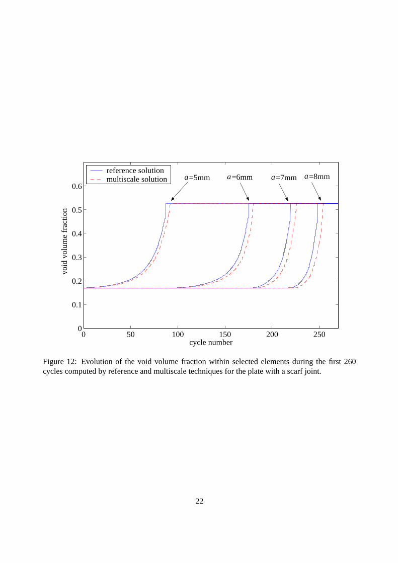
Figure 12 illustrates the evolution of void volume fraction within a number of selected elementsin front of the crack tip. The multiscale simulation was conducted using the algorithm parameters,EL = 4, δωωωall = 0.02,0.02, and with error tolerance,Etol = 0.0004,0.0005. Snapshots of thecrack growth history for the cycle-by-cycle and multiscale techniques are compared in Fig. 13. Agood agreement in the overall crack growth was observed between the reference and the multi-scale approach, despite some discrepancies in the void volume fraction growth in the individualelements. The simulated crack path under cyclic loading conditions was found to be somewhatsmoother compared to the test data under monotonic loading (Fig. 10). This trend is consistentwith experimental observations [54].

20

adherent

(elastic)

RME adhesive

(GTN model)

initial flaw

t(x,t,τ)-

Figure 11: Finite element mesh of the plate with a scarf joint.

21

0 50 100 150 200 2500

0.1

0.2

0.3

0.4

0.5

0.6

cycle number

void

vol

ume

frac

tion

reference solutionmultiscale solution a =5mm =6mm a =7mm a =8mm a

Figure 12: Evolution of the void volume fraction within selected elements during the first 260cycles computed by reference and multiscale techniques for the plate with a scarf joint.

22

c)

Figure 13: Crack propagation patterns of the plate with a scarf joint after (a) 97, (b) 161, (c) 267,and (d) 373 load cycles, as computed by the reference and multiscale techniques.

23

7 Conclusion

A multiscale fatigue model was developed within the new framework of the mathematical homog-enization theory for almost periodic fields. The almost-periodic operators have been introduced tocapture the long time response of inelastic solids subjected to short duration oscillatory loading.The proposed life prediction methodology was implemented in ABAQUS and has been found tobe in good agreement with the direct cycle-by-cycle simulations.

This work represents the first attempt in developing a simulation-based approach in the fieldwhere the design is dominated by experiments. Several theoretical issues, such as mesh sensitivity,as well as the critical issue of validation (against the experimental data) have not been addressedso far. These issues remain the focus of our future studies.

8 Acknowledgement

This work was supported by the Office of Naval Research through grant number N00014-97-1-0687. This support is gratefully acknowledged. Figure 10:c© Crown copyright 2004. Reproducedby permission of the Controller of HMSO.

References

[1] P. C. Paris and F. Erdogan. A critical analysis of crack propagation laws.J. Basic Engng.,85:528–534, 1963.

[2] M. H. El Haddad, T. H. Topper, and K. N. Smith. Prediction of non-propagating cracks.Engng. Fracture Mech., 11:573–584, 1979.

[3] W. Elber. Fatigue crack closure under cyclic tension.Engng. Fracture Mech., 2:37–45, 1970.

[4] R. G. Foreman, V. E. Keary, and R. M. Engle. Numerical analysis of crack propagation incyclic-loaded structures.J. Basic Engng., 89:459–464, 1967.

[5] M. Klesnil and P. Lukas. Influence of strength and stress history on growth and stabilisationof fatigue cracks.Engng. Fracture Mech., 4:77–92, 1972.

[6] O. E. Wheeler. Spectrum loading and crack growth.J. Basic Engng., 94:181–186, 1972.

[7] O. Nguyen, E. A. Repetto, M. Ortiz, and R. A. Radovitzky. A cohesive model of fatiguecrack growth.Int. J. Fracture, 110(4):351–369, 2001.

[8] K. L. Roe and T. Siegmund. An irreversible cohesive zone model for interface fatigue crackgrowth simulation.Engng. Fracture Mech., 70:209–232, 2003.

[9] J. L. Chaboche. Continuum damage mechanics I: General concepts & II: Damage growth,crack initiation and crack growth.J. Appl. Mech., 55:59–72, 1988.

[10] C. L. Chow and Y. Wei. A model of continuum damage mechanics for fatigue failure.Int. J.Fatigue, 50:301–306, 1991.

24

[11] J. Fish and Q. Yu. Computational mechanics of fatigue and life predictions for compositematerials and structures.Comp. Meth. Appl. Mech. Engng., 191:4827–4849, 2002.

[12] C. Oskay and J. Fish. Fatigue life prediction using 2-scale temporal asymptotic homogeniza-tion. Int. J. Numer. Meth. Engng., 2003. in print.

[13] M. Kaminski and M. Kleiber. Numerical homogenization of N-component composites in-cluding stochastic interface defects.Int. J. Numer. Meth. Engng., 47:1001–1027, 2000.

[14] G. W. Milton. The Theory of Composites. Cambridge Univ. Press, Cambridge, UK, 2002.

[15] S. Torquato.Random Heterogeneous Materials: Microstucture and Macroscopic Properties.Springer-Verlag, New York, 2002.

[16] K. Sab. On the homogenization and the simulation of random materials.Eur. J. Mech.,A/Solids, 11:585–607, 1992.

[17] J. Fish and A. Wagiman. Multiscale finite element method for a locally nonperiodic hetero-geneous medium.Comp. Mech., 12:164–180, 1993.

[18] S. Ghosh, K. Lee, and S. Moorthy. Multiple scale analysis of heterogeneous elastic structuresusing homogenization theory and Voronoi cell finite element method.Int. J. Solids Structures,32:27–62, 1995.

[19] S. Ghosh, K. Lee, and S. Moorthy. Two scale analysis of heterogeneous elastic-plastic ma-terials with asymptotic homogenization and Voronoi cell finite element method.Comput.Methods Appl. Mech. Engng., 132:63–116, 1996.

[20] J. T. Oden and T. I. Zohdi. Analysis and adaptive modeling of highly heterogeneous elasticstructures.Comput. Methods. Appl. Mech. Engng., 148:367–391, 1997.

[21] T. I. Zohdi, J. T. Oden, and G. J. Rodin. Hierachical modeling of heterogeneous bodies.Comput. Meth. Appl. Mech. Engng., 138:273–298, 1996.

[22] M.-J. Pindera, J. Aboudi, and S. M. Arnold. Limitations of the uncoupled, RVE-based mi-cromechanical approach in the analysis of functionally graded composites.Mechanics ofMaterials, 20:77–94, 1995.

[23] N. Ansini and A. Braides. Separation of scales and almost-periodic effects in the asymptoticbehavior of perforated media.Acta Applicandae Math., 65:59–81, 2001.

[24] A. Braides and A. Defranceschi.Homogenization of Multiple Integrals. Oxford Univ. Press,Oxford, 1998.

[25] G. Nguetseng and H. Nnang. Homogenization of nonlinear monotone operators beyond theperiodic setting.Electronic J. Diff. Eqn., 36:1–24, 2003.

[26] O. A. Oleinik, A. S. Shamaev, and G. A. Yosifian.Mathematical Problems in Elasticity andHomogenization. North-Holland Press, Amsterdam, 1992.

25

[27] V. V. Zhikov, S. M. Kozlov, and O. A. Oleinik.Homogenization of Differential Operatorsand Integral Functionals. Springer-Verlag, New York, 1994.

[28] V. Tvergaard. Material failure by void growth to coalescence.Adv. Appl. Mech., 27:83–151,1990.

[29] Z. P. Bazant, T. B. Belytschko, and T. P. Chang. Continuum theory for strain softening.J.Engng. Mech., 110:1666–1691, 1984.

[30] R. de Borst and L. J. Sluys. Localization in Cosserat continuum under static and dynamicloading conditions.Comput. Methods Appl. Mech. Engng., 90:805–827, 1991.

[31] R. de Borst and H. B. Muhlhaus. Gradient dependent plasticity: Formulation and algorithmicaspects.Int. J. Numer. Meth. Engng., 35:521–539, 1992.

[32] K. Garikipati and T. J. R. Hughes. A variational multiscale approach to strain localizationformulation for multidimensional problems.Comput. Methods. Appl. Mech. Engng., 188:39–60, 2000.

[33] J. C. Simo and J. Oliver. A new approach to the analysis and simulation of strain softening insolids. In Z. P. Bazant, Z. Bittnar, M. Jirasek, and J. Mazars, editors,Fracture and Damagein Quasibrittle Structures. 1994.

[34] A. Benssousan, J. L. Lions, and G. Papanicolaou.Asymptotic Analysis for Periodic Struc-tures. North-Holland, Amsterdam, 1978.

[35] D. Cioranescu and P. Donato.An Introduction to Homogenization. Oxford Univ. Press,Oxford, UK, 1999.

[36] A. L. Gurson. Continuum theory of ductile rapture by void nucleation and growth: Part I-yield criteria and flow rules for porous ductile media.J. Engng. Mater. and Technol., 99:2–15,1977.

[37] V. Tvergaard. Influence of voids on shear band instabilities under plane strain conditions.Int.J. Fracture, 17:389–407, 1981.

[38] V. Tvergaard. On localization in ductile materials containing spherical voids.Int. J. Fracture,18:237–252, 1982.

[39] C. C. Chu and A. Needleman. Void nucleation effects in biaxially stretched sheets.J. Engng.Mater. and Technol., 102:249–256, 1980.

[40] V. Tvergaard. Material failure by void coalescence in localized shear bands.Int. J. SolidsStructures, 18:659–672, 1982.

[41] M. E. Mear and J. W. Hutchinson. Influence of yield surface curvature on flow localizationin dilatant plasticity.Mech. Mater., 4:395–407, 1985.

[42] V. Tvergaard. Effect of yield surface curvature and void nucleation on plastic flow localiza-tion. J. Mech. Phys. Solids, 35(1):43–60, 1987.

26

[43] M. Gologanu, J.-B. Leblond, G. Perrin, and J. Devaux.Recent Extensions of Gurson’s Modelfor Porous Ductile Metals, chapter 2, pages 61–130. Springer-Verlag, 1997.

[44] V. Tvergaard and A. Needleman. Analysis of the cup-cone fracture in a round tensile bar.Acta Metall., 32(1):157–169, 1984.

[45] J. Llorca, S. Suresh, and A. Needleman. An experimental and numerical study of cyclicdeformation in metal-matrix composites.Metall. Trans. A, 23A:919–934, 1992.

[46] M. Ristinmaa. Void growth in cyclic loaded porous plastic solid.Mech. of Mater., 26:227–245, 1997.

[47] N. Aravas. On the numerical integration of a class of pressure-dependent plasticity models.Int. J. Numer. Meth. Engng., 24:1395–1416, 1987.

[48] J. H. Lee and Y. Zhang. On the numerical integration of a class of pressure-dependent plas-ticity models with mixed hardening.Int. J. Numer. Meth. Engng., 32:419–438, 1991.

[49] J. C. Simo and T. J. R. Hughes.Computational Inelasticity. Springer, New York, 1998.

[50] G. Dean, L. Crocker, B. Read, and L. Wright. Prediction of deformation and failure ofrubber-toughened adhesive joints.Int. J. Adhes. Adhes., 24:295–306, 2004.

[51] M. Imanaka and Y. Suzuki. Yield behavior of rubber-modified epoxy adhesives under multi-axial stress conditions.J. Adhesion Sci. Technol., 16(12):1687–1700, 2002.

[52] R. S. Kody and A. J. Lesser. Yield behavior and energy absorbing characteristics of rubber-modified epoxies subjected to biaxial stress states.Polym. Comp., 20:250–259, 1999.

[53] A. Lazzeri and C. B. Bucknall. Dilatation bands in rubber toughened plastics.J. Mater. Sci.,28:6799–6808, 1993.

[54] N. E. Frost, K. J. Marsh, and L. P. Pook.Metal Fatigue. Clarendon Press, Oxford, 1974.

27

A Micro- and macro-chronological evolution equations for theGTN model

The plastic loading parameter,H, is computed by considering a fictitious yield surface,ΦG [41, 42]:

ΦG = ΦG(σσσG, f ,σM) =(qG)2

σ2M

+2q1 f cosh

(−3

2q2

pG

σM

)−1− (

q1 f)2

(63)

and, choosing the fictitious stress components,σσσG, such that:

σσσG

σM=

ΘΘΘσF

(64)

The above equation ensures thatΦ = 0 impliesΦG = 0. The micro-chronological plastic strainrate tensor,µµµ,τ, is chosen to be equivalent to the associated fictitious plastic strain rate tensor,µµµG

,τ.Using (43), (45) and (64),H can be determined as:

H =−σM

σF

∂Φ∂ f

(1− f )(

δδδ :∂Φ∂σσσ

)+

[σM

σFA

∂Φ∂ f

+∂Φ∂σF

]Et

1− f1

σM

(ΘΘΘ :

∂Φ∂σσσ

)(65)

The macro-chronological consistency parameter,λo, is evaluated by setting the macro-chronologicalplastic strain rate tensor,µµµ,t to be equivalent to the associated fictitious plastic strain rate tensor,µµµG

,t .The micro- and macro-chronological evolution equations of void volume fraction, equivalent

plastic strain, matrix flow strength, and yield surface radius are obtained by substituting the statevariable and stress decompositions into (25), (26), (28), (29), and (22), matching the terms withrespect to their orders, and applying the PTH operator to the higher order equations. The originalevolution equation of the void volume fraction yields (for tensile loading):

O(ζ−1) : f,τ =(1−M( f )− f

)δδδ : µµµ,τ +A ρ,τ (66)

O(1) : f o,t = (1− f o)δδδ : µµµo

,t −⟨

f δδδ : µµµ1,t

⟩+ 〈A〉ρo

,t +⟨Aρ1

,t

⟩(67)

The micro-chronological evolution equation for the void volume fraction is given by (66). Ex-ploiting the dual decomposition relations, the evolution equation of void volume fraction for themacro-chronological problem yields:

M( f ),t =1ζ

⟨f,τ

⟩+ f o

,t =(1−M( f )−⟨

f⟩)

δδδ : M(µµµ),t −⟨

f δδδ :

(1ζ

µµµ,τ + µµµ,t

)⟩

+〈A〉M(ρ),t −⟨

A(

1ζ

ρ,τ + ρ,t

)⟩ (68)

Similarly, the original evolution equation for the equivalent plastic strain may be expressed interms of the decompositions given in (32):

O(ζ−1) : ρ,τ =

(M(ΘΘΘ)+ ΘΘΘ

): µµµ,τ[

1−M( f )− f][M(σF)+ σF ]

(69)

O(1) : ρo,t =

⟨ (M(ΘΘΘ)+ ΘΘΘ

)[1−M( f )− f

][M(σF)+ σF ]

⟩: µµµo

,t (70)

+

⟨ (M(ΘΘΘ)+ ΘΘΘ

): µµµ1

,t[1−M( f )− f

][M(σF)+ σF ]

⟩

28

The micro-chronological evolution equation for the equivalent plastic strain is given by (69). Themacro-chronological equation takes the form:

M(ρ),t =1ζ〈ρ,τ〉+ρo

,t =

⟨ (M(ΘΘΘ)+ ΘΘΘ

)[1−M( f )− f

][M(σF)+ σF ]

⟩: M(µµµ),t

+

⟨ (M(ΘΘΘ)+ ΘΘΘ

)[1−M( f )− f

][M(σF)+ σF ]

:

(1ζ

µµµ,τ + µµµ,t

)⟩ (71)

The evolution equations of the matrix flow strength and the yield surface radius may be ex-pressed as:

O(ζ−1) : σM,τ = Et ρ,τ; σF,τ = bσM,τ (72)

O(1) : σoM,t =

⟨Et⟩ρo

,t +⟨Etρ1

,t

⟩; σo

F,t = bσoM,t (73)

and,

M(σM),t =1ζ〈σM,τ〉+σo

M,t =⟨Et⟩M(ρ),t +

⟨Et

(1ζ

ρ,τ + ρ,t

)⟩(74)

M(σF),t =1ζ〈σF,τ〉+σo

F,t = bM(σM),t (75)

in which, (72a) and (74) are the micro- and macro-chronological evolution equations of the matrixflow strength, respectively. (72b) and (75) correspond to the evolution equations of the yield surfaceradius for the micro- and macro-chronological problems, respectively.

The consistency parameter for the kinematic hardening rule,ϑ, is decomposed using an expan-sion similar to the expansion ofλ:

ϑ(t,τ) =1ζ

ϑ1(t,τ)+ϑo(t) (76)

where,ϑ1, andϑo may be interpreted as the consistency parameters of the hardening rule inducedby the micro- and macro-chronological loadings, respectively. Applying (32) to the yield surfaceradius, inserting the resulting equation and (76) into (31), separating the terms with respect to theirorders, and applying (8) to the resultingO(1) equation, we obtain:

O(ζ−1) : ααα,τ = ϑ1(M(ΘΘΘ)+ ΘΘΘ

)(77)

O(1) : αααo,t = ϑoΘΘΘo (78)

The micro-chronological evolution equation for the center of the yield surface,ααα1, is given by (77).The micro-chronological consistency parameter,ϑ1, is evaluated using the consistency condi-tion (43):

ϑ1 = Q∂Φ∂σσσ

: σσσ,τ (79)

whereQ is expressed as:

Q = (1−b)(

ΘΘΘ :∂Φ∂σσσ

)−1[1+

σy

σF

1H

∂Φ∂ f

(1− f )

(δδδ :

∂Φ∂σσσ

)+

Et

1− f1

σF

(ΘΘΘ :

∂Φ∂σσσ

)](80)

29

The evolution equation for the macro-chronological yield surface center is evaluated using thedefinition of the APTH operator:

M(ααα),t =1ζ

⟨ϑ1(

M(ΘΘΘ)+ ΘΘΘ)⟩

+ϑo(M(ΘΘΘ)+

⟨ΘΘΘ

⟩)(81)

The macro-chronological consistency parameter for the hardening rule,ϑo, is evaluated by apply-ing the PTH operator to (44):

ϑo =⟨

Q∂Φ∂σσσ

⟩: M(σσσ),t +

⟨Q

∂Φ∂σσσ

: σσσ,t

⟩(82)

30