MULTISCALE MODEL. SIMUL. c© 2016 Society for Industrial and Applied MathematicsVol. 14, No. 4, pp. 1463–1487

ON A SCHRÖDINGER–LANDAU–LIFSHITZ SYSTEM:VARIATIONAL STRUCTURE AND NUMERICAL METHODS∗

JINGRUN CHEN† , JIAN-GUO LIU‡ , AND ZHENNAN ZHOU§

Abstract. From a variational perspective, we derive a series of magnetization and quantum spincurrent systems coupled via an “s-d” potential term, including the Schrödinger–Landau–Lifshitz–Maxwell system, the Pauli–Landau–Lifshitz system, and the Schrödinger–Landau–Lifshitz systemwith successive simplifications. For the latter two systems, we propose using the time splittingspectral method for the quantum spin current and the Gauss–Seidel projection method for themagnetization. Accuracy of the time splitting spectral method applied to the Pauli equation isanalyzed and verified by numerous examples. Moreover, behaviors of the Schrödinger–Landau–Lifshitz system in different “s-d” coupling regimes are explored numerically.

Key words. Landau–Lifshitz equation, Schrödinger equation, Pauli equation, time splittingspectral method, variational structure

AMS subject classifications. 65M70, 78A25, 82C10

DOI. 10.1137/16M106947X

1. Introduction. Magnetic materials have been successfully used to record andstore data for a long time. These materials produce their own persistent magneticorders even in the absence of an external magnetic field. Magnetization is the vectorfield which describes the intrinsic magnetic order. Its dynamics was first modeledby Landau and Lifshitz in 1935 [18]. Even though the Landau–Lifshitz equation isa phenomenological model, it is still widely used in micromagnetics [4, 13]. While arigorous microscopic derivation of the equation is still lacking, magnetization dynamicscan be viewed as the collective dynamics of atomic magnetic moments.

In recent years, various techniques have been developed to ease magnetization re-versal and switching; see [3, 14, 23] for examples and references therein. One effectiveway is to control the spin degrees of freedom (dofs) of electrons, which in turn affectthe dynamics of magnetization. This is known as spin transfer torque (STT), observedindependently by Fert [1] and Grünberg [11]. The presence of STT can reduce thecharacteristic time scale of data recording and storage processes by orders of magni-tude. Models at different levels are proposed to understand magnetization dynamicsin the presence of spin dofs. Numerous models have been developed to describe thedynamics of spin. One type of model adds an additional torque accounting for spindynamics in the Landau–Lifshitz equation; see, for example, [8, 26]. The other typeof model treats spin dynamics and magnetization dynamics on an equal footing; see,for example, [7, 22, 25]. In [25], linear response theory is used to derive a diffusion

∗Received by the editors April 6, 2016; accepted for publication (in revised form) September 27,2016; published electronically December 6, 2016.

http://www.siam.org/journals/mms/14-4/M106947.htmlFunding: The first author acknowledges support from the Young Thousand Talents Program of

China and National Natural Science Foundation of China via grant 21602149. The second author ispartially supported by KI-Net NSF RNMS grant 1107291 and NSF grant DMS 1514826. The thirdauthor is partially supported by RNMS11-07444 (KI-Net).†Mathematical Center for Interdisciplinary Research and School of Mathematical Sciences, Soo-

chow University, Suzhou 215006, China (jingrunchen@suda.edu.cn).‡Department of Mathematics and Department of Physics, Duke University, Box 90320, Durham

NC 27708 (jliu@phy.duke.edu).§Department of Mathematics, Duke University, Box 90320, Durham NC 27708 (zhennan@

math.duke.edu).

1463

1464 JINGRUN CHEN, JIAN-GUO LIU, AND ZHENNAN ZHOU

equation for spin dynamics. A more microscopic justification for the diffusion-typeequation is derived from the Boltzmann equation in [22]. Connections between thesetwo types of models are made under certain assumptions [26].

In [7], a Schrödinger equation in the spinor form was used to model spin atthe quantum level. Using the Wigner transform and moment closure, the authorsderived a diffusion equation for spin dynamics. It recovers the model in [25] in theregime of weak spin-magnetization coupling. The model has been successfully used formagnetization switching [7] and domain wall dynamics [6] with both qualitative andquantitative agreements with experimental results. The passage from the Schrödingerequation to the diffusion equation relies on three main assumptions: (1) a BGK-typeoperator for the relaxation term in the Boltzmann equation; (2) certain momentclosure to get a closed spin-magnetization coupled system; and (3) a quasi-staticapproximation to get the constitutive relation between the applied current densityand the spin current density. These assumptions are difficult to verify except thelast one, since its validity comes from the diffusive regime which can be checked frommaterial constants.

Nevertheless, spin dynamics in the general case will be of great interest due toits universality. Therefore, we shall consider the Schrödinger equation in the spinorform and couple it to the Landau–Lifshitz equation. The purpose of the currentpaper is two-fold: (1) derive the coupled system and its analogue from a variationalperspective (2) propose efficient algorithms for the coupled system and its analogue.In subsequent papers, we will analyze the variational models and show the existenceof (weak) solutions. As a byproduct, we propose the time splitting spectral methodfor the Pauli equation, and rigorous convergence results are presented. This methodhas spectral accuracy in space and, in theory, high order temporal accuracy can benaturally achieved by the operator splitting method. It also allows large time stepsto compute correct physical observables, which is ideal for hybrid simulation. Thetime splitting spectral method for the Pauli equation itself is of significance in termsof numerical analysis and scientific computations.

The rest of the paper is organized as follows. We derive the Schrödinger–Landau–Lifshitz–Maxwell system from a space-time total action, and the Pauli–Landau–Lifshitz system from a free energy formulation in section 2, where the Schrödinger–Landau–Lifshitz system can be considered as a simplified model of either case. Insection 3, the time splitting spectral method for the Pauli equation is given analyzed indetail, and the Gauss–Seidel projection method of the Landau–Lifshitz equation is re-viewed. Extensive numerical tests are provided in section 4, some of which are devotedto carefully verifying the numerical properties of the time splitting spectral method tothe Pauli equation, while the rest are numerical examples of the Schrödinger–Landau–Lifshitz system in different coupling regimes.

2. Models and variational structures. In this section, we first describe thesemiclassical spin dynamics by the Schrödinger equation in the spinor form coupledwith the Landau–Lifshitz equation. The total space-time action is introduced to derivethe Pauli–Landau–Lifshitz–Maxwell system and the Pauli–Landau–Lifshitz system isderived from construction of the free energy, whereas the Schrödinger–Landau–Lifshitzsystem can be viewed as a simplified model from each scenario.

2.1. The Schrödinger–Landau–Lifshitz system. For x ∈ R3 and t ∈ R,we denote the quantum wavefunction for spin ± 1

2 electrons by ψ(x, t) ∈ C2 and themagnetization by m(x, t) ∈ R3. The Schrödinger–Landau–Lifshitz system reads as

ON A SCHRÖDINGER–LANDAU–LIFSHITZ SYSTEM 1465

iε∂tψ(x, t) = −ε2

2∆xψ(x, t) + V (x)ψ(x, t)− ηm(x, t) · σψ(x, t), x ∈ R3,(1)

∂tm(x, t) = −m(x, t)× (Heff + ηs(x, t))

− αm(x, t)× (m(x, t)× (Heff + ηs(x, t))), x ∈ Ω,(2)

ψ(x, 0) = ψ0(x), x ∈ R3,(3)m(x, 0) = m0(x), x ∈ Ω.(4)

Here Ω is the domain occupied by the magnetic material. The effective field Heff hasthe form

(5) Heff = ∆m− (m2e2 +m3e3) + (Hs +H0)

and can be calculated as − δFLLδm , where FLL is the Landau–Lifshitz energy given by

(6) FLL =1

2

ˆΩ

(m2

2 +m23

)+

1

2

ˆΩ

|∇m|2 − 1

2

ˆΩ

Hs ·m−ˆ

Ω

H0 ·m.

Due to the presence of the spin density s, it is natural to introduce the modifiedeffective field

(7) Heff = Heff + ηs.

In (5), ej3j=1 are the standard bases of R3. In (2), ηs plays as an additionaltorque. H0 is the externally applied magnetic field and Hs is the stray field given byHs = −∇U , where U satisfies

(8) U(x) =

ˆΩ

∇N(x− y) ·m(y, t) dy

with N(x) = −1/(4π|x|) denoting the Newtonian potential.Here, (1) is the one-body Schrödinger equation, in which ψ = (ψ+, ψ−)T is

called the spinor, ε ∈ (0, 1] is the semiclassical parameter, V (x) is the external scalarpotential, and σ = σxe1 + σye2 + σze3 gives the Pauli matrices

σx =

(0 11 0

), σy =

(0 −ii 0

), σz =

(1 00 −1

).

The last term in the Hamiltonian of the Schrödinger equation describes the spin-magnetization interaction, i.e., the coupling between spin dofs of the applied currentand magnetization. η is the corresponding coupling strength. This model neglectsthe self-induced electromagnetic fields generated by the applied current.

To extract macroscopic quantities, we define the density matrix

D = ψψ† =

(ψ+ψ+ ψ+ψ−ψ−ψ+ ψ−ψ−

),

then the associated position density ρ is defined as

ρ(x, t) = TrD = ψ+ψ+ + ψ−ψ−

and the spin density s is defined as

s(x, t) = TrDσ = TrDσxe1 + TrDσye2 + TrDσze3.

1466 JINGRUN CHEN, JIAN-GUO LIU, AND ZHENNAN ZHOU

From (1), by direct calculation, the total mass of the quantum wavefunction, denotedby

‖ψ‖(t) =

(ˆR3

|ψ+(x, t)|2 + |ψ−(x, t)|2dx) 1

2

,

is conserved, i.e.,d

dt‖ψ‖ = 0.

As for the magnetization dynamics (2), the magnetization m(x, t) is normalized|m| = 1 in the pointwise sense over Ω. A Neumann boundary condition is imposedfor (2):

∂m

∂ν= 0 on ∂Ω,

where ν is the unit normal vector on the domain boundary ∂Ω.By taking the inner product with m, (2) becomes

∂t|m|2 = 0,

where we have used the fact that both terms on the right-hand side of (2) are per-pendicular to m. Hence, in the Schrödinger–Landau–Lifshitz system, both ψ and mstay normalized through time evolution. It is worth mentioning that the second termin (2) is known as the Gilbert damping [9], where α > 0 is the damping constant.

This particular type of spin-magnetization interaction is the so-called “s-d” cou-pling model [7, 8], which is relatively well studied and widely used in the physicscommunity. There are extensive experimental studies for many magnetic devices [14].Other effects, such as the Rashba spin-orbit coupling and the Dzyaloshinskii–Moriyainteraction, are also of great significance. These will also be considered in subsequentpapers.

2.2. The total action and the Schrödinger–Landau–Lifshitz–Maxwellsystem. In this section, we aim to formulate the Schrödinger–Landau–Lifshitz–Maxwell system with the least action principle by constructing the total action. Pre-viously, the variational structure of the Schrödinger equation has been widely knownand well studied, and various Landau–Lifshitz models have been derived by the leastaction principle or the free energy approach (the reader may refer to [12] for a generaldiscussion). However, the formulation becomes more challenging when the magneticfield is complicated, for example, when the self-induced electromagnetic field is con-sidered, or when the external magnetic field is dominant. We aim to discuss thesescenarios in the following, emphasizing their relations to the simplified Schrödinger–Landau–Lifshitz system.

For simplicity, we suppress the appearance of the parameters, since for the varia-tion problem we only consider the case when all the parameters are fixed. In general,we consider the Schrödinger–Landau–Lifshitz–Maxwell action, which consists of theSchrödinger part SS, the Landau–Lifshitz part SLL, the Maxwell part Sm, and thespin-magnetization coupling part SC:

S = SS + SLL + Sm + SC,

where

SS =

ˆΩ

dx

ˆdt

[Re(iψ∂ψ

∂t− ϕ|ψ|2

)− 1

2|−i∇xψ −Aψ|2 − V (x)|ψ|2

],

ON A SCHRÖDINGER–LANDAU–LIFSHITZ SYSTEM 1467

Sm =

ˆR3

dx

ˆdt

1

2

(∣∣∣∣∂A∂t +∇ϕ∣∣∣∣2 − |∇ ×A−m|2

),

SLL = −ˆdtFLL,

andSC =

ˆΩ

dx

ˆdt s ·m.

Note that SS, SLL, and SC are defined on the material domain Ω, while Sm is definedon the whole space R3 since the electromagnetic field is induced even outside thematerial. Here A is the electromagnetic vector potential and ϕ is the self-inducedscalar potential. To clarify the notation, we use

|−i∇xψ −Aψ|2 = |−i∇xψ+ −Aψ+|2 + |−i∇xψ− −Aψ−|2 ,

which is a scalar. In the above expressions, SS includes the time derivative contribu-tion, the modified kinetic term, the electric scalar potential term, and the externalpotential term. SLL describes the Landau–Lifshitz part. Sm includes the electric fieldcontribution and the magnetic field contribution. SC describes the coupling betweenthe charged current and the magnetization of the ferromagnetic material by the “s-d”model.

In the absence of the Schrödinger equation, the action S = Sm + SLL with re-spect to ϕ, A, and m gives the Landau–Lifshitz–Maxwell system; see [12]. Withthe presence of the polarized current described by the Schrödinger equation and dueto the self-induced electromagnetic field, the vector potential modifies the quantummomentum operator by

−i∇ → −i∇−A,

which is referred to as the Peierls substitution [20, 21]. Also, the polarized currentgenerates a spin density s, which modifies the dynamics of the magnetization. Forsimplicity, we only keep a first order correction with respect to s, given by SC. In otherwords, SC defines the interaction between the spin current and the magnetization inthe system.

By taking variations with respect to ψ, A, ϕ, and m, one can derive the cou-pled Schrödinger equation, the Maxwell equations, and the Landau–Lifshitz equation,respectively. Note that, although the vector potential A contains the partial contri-bution from the magnetization m, we treat these two as independent variables.

The Schrödinger equation is obtained by the least action principle

δS

δψ= 0,

which leads to

i∂tψ =1

2(−i∇x −A)

2ψ + (ϕ+ V )ψ −m(x, t) · σψ(x, t).

Next, to obtain the Maxwell equations, we consider the following two variationalequations:

δS

δϕ= 0,

δS

δA= 0.

1468 JINGRUN CHEN, JIAN-GUO LIU, AND ZHENNAN ZHOU

Then, we get

(9) ∇ ·(∂A

∂t+∇ϕ

)= −ρ,

(10) ∇× (∇×A−m) +∂

∂t

(∂A

∂t+∇ϕ

)= j,

wherej = Im(ψ†∇ψ)−Aρ

is the flux density.We use the change of variables

E = −(∂A

∂t+∇ϕ

),

B = ∇×A, B = H + m

and immediately get

(11) ∇×E + ∂tB = 0,

(12) ∇ ·B = 0.

Also, (9) and (10) can be written as

(13) ∇ ·E = ρ,

(14) ∇×H− ∂tE = j.

Therefore, E and B can be interpreted, respectively, as the electric and the magneticfield. Equations (11), (12), (13), and (14) are precisely the Maxwell equations.

As in the original derivation of the Landau–Lifshitz equation, we cannot use theleast action principle. Instead, we can first compute the modified effective field andthen write the Landau–Lifshitz equation in the same way as in [18]:

Heff =δS

δm, ∂tm = −m× Heff − αm×

(m× Heff

).

2.3. Regarding the self-induced electromagnetic field. In general, in theabsence of the external magnetic field, the H field has two sources: the self-inducedfield of the magnetization and the self-induced field by the charged current. In prac-tice, the self-induced electromagnetic field can be neglected. In that case, the H fieldreduces to the stray field, or the demagnetization field, denoted by Hs. The magneticenergy reduces to the stray field energy

1

2

ˆR3

dx|Hs|2.

To clarify the relations between the magnetic field B, the magnetization m, andthe stray field Hs, we carry out the following heuristic arguments. Inside the ferro-magnetic material, the magnetic field B consists of two parts:

(15) B = Hs +m.

ON A SCHRÖDINGER–LANDAU–LIFSHITZ SYSTEM 1469

But outside the material, the magnetic field B reduces to the stray field Hs. By theMaxwell equations, we obtain that

(16) ∇ ·B = 0, ∇×Hs = 0.

The second equation implies Hs = −∇U for some scalar function U , often referred toas the magnetostatic potential. Then the first equation in (16) can be rewritten as

∇ · (−∇U + m) = 0, x ∈ R3,

which shall be understood in the sense of distributions, i.e., U ∈ H1(R3) satisfies, forarbitrary test function u ∈ H1(R3),

(17)ˆR3

∇U · ∇u dx =

ˆΩ

m · ∇u dx.

This explains why the stray field Hs can be solved by solving the magnetostaticpotential (8). The reader may refer to [4] for more details.

We want to point out that the formulation above can be viewed as the Helmholtzdecomposition of the zero extension of the magnetization m to R3. With a bit ofabuse of notation, we would still denote the extension of the magnetization by m.

By Helmholtz’s theorem, the vector field m : R3 → R3 can be resolved into thesum of an irrotational vector field and a divergence-free vector field

m = B−Hs, ∇ ·B = 0, ∇×Hs = 0.

Due to the zero extension of the magnetization from Ω to R3, the decomposition hasto be viewed in a weak sense, and the scalar potential of the divergence-free vectorfield is obtained by (17).

Moreover, with the curl-free part Hs defined in (17), the divergence-free part Bis defined simultaneously by B = m + Hs. One can easily check that the condition∇ ·B = 0 is satisfied automatically.

2.4. The free energy and the Pauli–Landau–Lifshitz system. In the pre-vious part, we formulated the coupling model between the magnetization and thequantum spin density with interplay of the self-induced electromagnetic waves. Inthis section, we aim to explore a different scenario, that is, when the interaction be-tween the magnetization and the quantum spin density is exposed to strong externalelectromagnetic fields.

In the presence of the external scalar potential V and the vector potential A, weneglect the self-induced electromagnetic field, and consider the Pauli–Landau–Lifshitzfree energy

(18) F =

ˆΩ

[1

2|−i∇xψ −Aψ|2 + V |ψ|2 − s · (m+ H)

]dx+ FLL.

In this formulation, the external electromagnetic field is dominant, and thus the scalarand vector potentials no longer satisfy the Maxwell equations. The free energy consistsof the quantum kinetic energy, the quantum potential energy, the Landau–Lifshitzenergy, and the spin magnetic field coupling energy.

Here, since the dominant magnetic field is treated as a prescribed function, thevector potentialA itself is not considered an independent variable. The total magneticfield B = ∇ ×A = m + H consists of the background magnetization m and the H

1470 JINGRUN CHEN, JIAN-GUO LIU, AND ZHENNAN ZHOU

field, where m is still an independent variable since its dynamics is governed by theLandau–Lifshitz equation. In theory, the H field includes the stray field and theexternal magnetic field, but we assume it is dominated by the external field, and wetreat it as a given function. That is why we do not include the magnetic field energyin (18).

The Pauli (Schrödinger–Pauli) equation is obtained by

i∂tψ =δFδψ

=1

2(−i∇x + A)

2ψ + Vψ − σ ·Bψ,(19)

where σ ·Bψ is the so-called Stern–Gerlach term. Equivalently, we can write the Pauliequation as

i∂tψ =1

2(σ · (−i∇x + A))

2ψ + Vψ.

In the Landau–Lifshitz equation, the modified effective field Heff can be obtainedin the same way as before, i.e., Heff = − δF

δm . Therefore, we have obtained the Pauli–Landau–Lifshitz system coupled by the spin magnetic field interaction.

2.5. The simplified model. So far, we have defined the total action which leadsto the Schrödinger–Landau–Lifshitz–Maxwell system and the free energy which leadsto the Pauli–Landau–Lifshitz system. To obtain the Schrödinger–Landau–Lifshitz sys-tem, we could either switch off the external magnetic field in the Pauli–Landau–Lifshitz system, i.e., reduce the spin magnetic field coupling energy to thespin-magnetization interaction energy, or we could neglect the self-induced electro-magnetic field in the Schrödinger–Landau–Lifshitz–Maxwell system. We further ex-plain the former approach in the following and the latter can be done in a similarfashion.

Assume that the self-induced electromagnetic field is negligible. The total energyfunctional of the Schrödinger–Landau–Lifshitz system simplifies to

F =

ˆΩ

1

2|−iε∇xψ|2 + V (x)|ψ|2dx+ FLL −

ˆΩ

ηs ·mdx.

In other words, we only keep the kinetic and potential energy of the charged current,the Landau–Lifshitz energy, and the spin-magnetization coupling energy. Here, wehave rescaled the quantum kinetic operator to −iε∇x for ε ∈ (0, 1]. When ε 1, thewavefunction of the charged current is in the highly oscillatory regime, which presentschallenges both in analysis and computation. Also, the coupling strength η is includedin the spin magnetic field coupling energy, which is an ad hoc parameter which maycome from the procedure of nondimensionalization [6, 7].

Finally, we are ready to derive the system (1)–(2). Obviously, the effective fieldHeff can be obtained by

Heff = − δFδm

= Heff + ηs.

Also, by direct calculation, the Schrödinger equation (1) can be rewritten as

iε∂tψ =δFδψ

= Hψ = −ε2

2∆xψ(x, t) + V (x)ψ(x, t)− ηm(x, t) · σψ(x, t).

Similarly, we have

iε∂tψ =δFδψ

= Hψ.

ON A SCHRÖDINGER–LANDAU–LIFSHITZ SYSTEM 1471

Next, we show that the total energy F is nonincreasing in time. A straightforwardcalculation produces

d

dtF =

ˆΩ

(δFδψ· ∂tψ +

δFδψ· ∂tψ +

δFδm· ∂tm

)dx

=

ˆΩ

(2Re

[δFδψ· ∂tψ

]+δFδm· ∂tm

)dx

=

ˆΩ

(δFδm· ∂tm

)dx.

In the last line, we use the fact that δFδψ · ∂tψ = 1

iε |Hψ|2 is purely imaginary.

For the remaining term, we calculate that

δFδm· ∂tm = −Heff · ∂tm

= αHeff · (m× (m× Heff))

= α(m× Heff) · (Heff ×m)

= −α∣∣∣m× Heff

∣∣∣2 .Finally, we conclude that

d

dtF = −α

ˆΩ

∣∣∣m× Heff

∣∣∣2 dx 6 0.

3. Numerical methods.

3.1. Time splitting spectral method for the Pauli equation. In theSchrödinger–Landau–Lifshitz system, the Schrödinger equation (1) can be consid-ered as a simplified version of the Pauli equation (19), where the vector potential Avanishes and the magnetic field B reduces to the magnetization m. In this section,we propose a time splitting spectral method (see [2, 15, 16, 19]) for the Pauli equationin the semiclassical regime

iε∂tψ =1

2(−iε∇x + A)

2ψ + Vψ − ησ ·Bψ,(20)

where the vector potential A and the scalar potential V are prescribed functions, andthe magnetic field B is given by

(21) B = ∇×A.

For simplicity, we assume A and V are time-independent functions. The extension totime-dependent potential cases is straightforward.

Here, the coefficient η defines the strength of the Stern–Gerlach term, which isreminiscent of the “s-d” coupling strength in the Schrödinger–Landau–Lifshitz system.We aim to design a numerical method for the system for wide ranges of parametersε and η. In particular, the method should work for the semiclassical regime, namely,ε 1 and for the strong coupling regime, namely, η = O(1).

Without loss of generality, we assume the Coulomb gauge ∇ ·A = 0; the Pauliequation can be formulated as

(22) iε∂tψ = −ε2

2∆ψ + iεA · ∇ψ +

(1

2|A|2 + V − ησ ·B

)ψ.

1472 JINGRUN CHEN, JIAN-GUO LIU, AND ZHENNAN ZHOU

By the operator splitting technique, for every time step t ∈ [tn, tn+1], one solves thekinetic step

(23) iε∂tψ = −ε2

2∆ψ, t ∈ [tn, tn+1],

followed by the potential step

(24) iε∂tψ =

(1

2|A|2 + V − ησ ·B

)ψ, t ∈ [tn, tn+1],

and followed by the convection step

(25) ∂tψ = A · ∇ψ, t ∈ [tn, tn+1].

For clarity, we rewrite the equation as

(26) ∂tψ = (A+ B + C)ψ,

where

A =iε

2∆, B = − i

ε

(1

2|A|2 + V − ησ ·B

), and C = A · ∇.

For simplicity, we consider the Pauli equation in one dimension with periodicboundary conditions. The extension to multidimensional cases is straightforward.In the one-dimensional case, the vector potential A reduces to a scalar function, sothe relation (21) is no longer satisfied. Hence, to demonstrate the construction of thenumerical method, we supposeB to be a three-component vector which is independentof A.

We assume, on computation domain [a, b], a uniform spatial grid xj = a + j∆x,j = 0, . . . , N − 1, where N = 2n0 , n0 is a positive integer, and ∆x = b−a

N . We alsoassume uniform time steps tk = k∆t, k = 0, . . . ,K. The construction of numericalmethods is based on the following (first order) operator splitting technique.

Let ψ(tn) be the exact solution at t = tn, which implies

ψ(tn+1) = e(A+B+C)∆tψ(tn).

Let ψnj be the numerical approximation of ψ(xj , tn) and let ψn be the numericalapproximation of ψ(tn), which means ψn has ψnj as its components.

Define the solution obtained by the (first order) operator splitting (without spatialdiscretization) as

(27) wn+1 = eC∆teB∆teA∆tψ(tn).

Note that wn+1 differs from ψ(tn+1) due to the operator splitting error.After operator splitting, the kinetic step can be solved analytically in time in the

Fourier space:

(28) ψ∗j =1

N

N/2−1∑l=−N/2

e−iε∆tµ2l /2ψ

n

l eiµl(xj−a),

ON A SCHRÖDINGER–LANDAU–LIFSHITZ SYSTEM 1473

where ψn

l are Fourier coefficients of ψnj defined by

ψn

l =

N−1∑j=0

ψnj e−iµl(xj−a), µl =

2πl

b− a, l = −M

2, . . . ,

M

2− 1.

For the potential step, due to the presence of σ · B, the whole potential is a2× 2 matrix. Fortunately, we have the following identity for the exponential of Paulimatrices, for any ~a = an, |n| = 1:

eia(n·σ) = I cos a+ i(n · σ) sin a,

which is analogous to Euler’s formula. I is the 2 × 2 identity matrix. Thus, by themethod of integration factor, we can derive the explicit solution of the potential step:(29)

ψ∗∗j = exp

(− i∆t

ε

(1

2|Aj |2 + Vj

))(I cos

(∆tη|Bj |

ε

)+ i(Bj · σ) sin

(∆tη|Bj |

ε

))ψ∗j .

Here, we denote

A(xj) = Aj , B(xj) = Bj = |Bj |Bj , and V (xj) = Vj .

Since we have used the analytical solutions in the kinetic step and in the potentialstep, there is no numerical error in time discretization of these two substeps.

In general, if we consider the potential step with a time-independent Hermitianmatrix potential M, we have

(30) iε∂tψ = Mψ, t ∈ [tn, tn+1].

In particular, we can obviously check that 12 |A|

2 +V −ησ ·B is Hermitian. Moreover,we express the analytical solution as

ψ(tn+1) = exp

(− iM∆t

ε

)ψ(tn).

Numerically, this matrix exponential can be computed by the eigenvalue decomposi-tion with minimal error. However, in the Pauli equation, or when the matrix potentialconsists of the Pauli matrices, the analytical expression (29) is superior in both effi-ciency and accuracy.

For the convection step, however, there is no obvious way to solve it analyticallybased on discrete data for a variable A(x). We propose a semi-Lagrangian method tosolve the convection equation (25) as in [16, 19].

This method consists of two parts: backward characteristic tracing and interpo-lation. We compute the data ψn+1

j by first tracing backwards along the characteristicline

(31)dx(t)

dt= −A (x(t)) , x(tn+1) = xj ,

for time interval [tn, tn+1]. Denote x(tn) = x0j , obtained by numerically solving the

ODE (31) backwards in time as shown in Figure 1.We call the point set

x0j

the shifted point set. By the method of characteristics,

ψn+1j = ψ∗∗

(x0j

). But ψ∗∗

(x0j

)in general are not known, since x0

j are not necessarily

1474 JINGRUN CHEN, JIAN-GUO LIU, AND ZHENNAN ZHOU

tn

tn+1

xj−10 x

j0 x

j+10

xj−1

xj−1

xj

xj+1

xj

xj+1

Fig. 1. Backward tracing: xj are the grid points; x0j are the shifted grid points, which are thesolutions to problem (31) backwards in time at t = tn; and the dotted line indicates characteristics.

grid points. Therefore, interpolation is needed to approximate ψn+1j = ψ∗∗

(x0j

)based

on ψ∗∗. We compare the following two choices: the spectral interpolation and theMth order polynomial interpolation.

For the spectral approximation, the interpolant ΠNψ∗∗(x) =

∑N/2−1k=−N/2 cke

ikx isa global approximation to ψ∗∗(x) based on ψ∗∗. One needs O(N logN) operations toget the Fourier coefficients ck via the FFT method. But one needs O(N) operations toevaluate the interpolant at each point x0

j , since the shifted points x0j are not necessarily

the grid points, which means the inverse FFT does not apply. Hence, the total costis O(N2) in each time step. This will make the whole scheme very costly. However,one can make use of the recently developed methodology nonuniform FFT (NUFFT)(see [10]) to implement this interpolation with O(N logN) cost. The details of thisimplementation and the corresponding stability analysis have been given in [19].

For the Mth order Lagrange polynomial interpolation, one needs to establish apolynomial interpolant for each shifted point x0

j with the discrete data on the closestM grid points xj1 , . . . , xjM . For each shifted point x0

j , one uses M grid points near x0j

to form a Lagrange polynomial interpolant to approximate U(x0j ) with error of order

O(∆xM ). But certain stability constraints need to be satisfied for different interpo-lation methods. The extensive stability study of this method has been carried out in[16]. The total cost of the semi-Lagrangian method with the polynomial interpolationis O(N) for each time step.

By either interpolation option, we have shown that the method for the convectionstep is unconditionally stable. In the following, we continue our analysis with thespectral interpolation option. The analysis with polynomial interpolations can becarried out in a similar fashion. For simplicity, we name this method the first ordertime splitting spectral (TSSP) method.

We conclude this section with the following remark.

Remark 3.1. The first order operator splitting implies first order convergence intime. One can make use of Strang’s splitting to obtain a second order time dis-cretization method. If one wants to apply the second order Strang’s splitting to threeoperators, one can first group A + B together as a single operator, and then applyStrang’s splitting to A+B and C, while in the steps corresponding to A+B, one alsouses Strang’s splitting.

3.2. Error analysis of the TSSP method. To analyze the convergence of theTSSP method for the Pauli equation, it is worth noting that the Pauli equation andthe Schrödinger equation with vector potential share many similarities. The TSSP

ON A SCHRÖDINGER–LANDAU–LIFSHITZ SYSTEM 1475

method for the Schrödinger equation has been analyzed in [16, 19], so we will onlyhighlight the differences.

We further assume that the wavefunctions are ε-oscillatory in space and time butthe potentials are not oscillatory. So there are t, ε, x independent positive constantsCm that

(32)∥∥∥∥ ∂m1+m2

∂xm1∂tm2ψ±(t, ·)

∥∥∥∥C([0,T ];L2(a,b)) 61

εm1+m2Cm1+m2 ,

(33)∥∥∥∥ ∂m∂xmA

∥∥∥∥ L2(a,b) 6 Cm,

∥∥∥∥ ∂m∂xmV∥∥∥∥ L2(a,b) 6 Cm

(34)∥∥∥∥ ∂m∂xmBl

∥∥∥∥ L2(a,b) 6 Cm, l = 1, 2, 3.

Note that the differentiation operator is unbounded for general smooth func-tions, but it is bounded in the subspace of smooth L2 functions which are at mostε-oscillatory.

Since in the Pauli equation there is the additional Stern–Gerlach term, we needto study the resulting error in the operator splitting. We show, by studying thecommutators between the three operators in (26), when the potentials are spatiallyvariant, that the local splitting error in the first order splitting (23)–(25) for (22) is

(35) ψ(tn+1)− wn+1 = ψ(tn+1)− eC∆teB∆teA∆tψ(tn) = O

(∆t2

ε

).

Clearly, the exact solution to (22) at t = tn+1 with initial data ψ(tn) is given by

ψ(tn+1) = e(A+B+C)∆tψ(tn).

The operator splitting error results from the noncommutativity of the operators A,B, and C. In previous literature (see [2, 16]), the commutator was analyzed for scalarSchrödinger equations. The Pauli equation, on the other hand, is in the vector form,whereas the kinetic part A and the convection part C are still scalar operators. Butin the potential part, due to the presence of σ ·B, the total potential is in a Hermitianmatrix. As in [16, 19], it was shown that

[A∆t, C∆t]ψ = O

(∆t2

ε

),

where [·, ·] denotes the commutator. Direct computation gives

[A∆t, B∆t]ψ = (∆t)2

[1

2(∆xM) +

1

2∂xM∂x

]ψ = O

(∆t2

ε

),

[B∆t, C∆t]ψ = (∆t)2

(− iε

)(A∂xM)ψ = O

(∆t2

ε

),

where again we denote

M =1

2|A|2 + V − ησ ·B.

1476 JINGRUN CHEN, JIAN-GUO LIU, AND ZHENNAN ZHOU

Therefore, we have formally shown that the local operator splitting error is O(∆t2

ε )as in (35). Actually, the proof can be made completely rigorous if we give moreassumptions on the wavefunction and the potentials similar to those in [2, 16, 19].

We use fI to denote the spectral approximation based on the discrete data fj orf(xj). Now we are ready to state the following error estimate for the first order TSSPmethod. The proof will be very similar to those in [2, 16, 19], except for the splittingerror analysis which we have presented. Therefore, we would like to omit the proof.

Theorem 3.1. Let ψ(t, x) be the exact solution of (22) and let ψn be the dis-crete approximation by the first order TSSP method. We assume that the character-istic equations (31) are numerically solved with minimal error in the preprocessedstep, and that the spectral interpolation with the NUFFT technique is taken in thesemi-Lagrangian method for the convection step, where the extra error introduced byNUFFT is negligible. Under assumption (34), we further assume ∆x/ε = O(1) and∆t/ε = O(1); then, for all positive integers m > 1 and t ∈ [0, T ],

(36) ||ψ(tn)−ψnI ||L2 6 GmT

∆t

(∆x

ε

)m +

CT∆t

ε,

where C is a positive constant independent of ∆t, ∆x, ε, m, and M , and Gm arepositive constants independent of ∆t, ∆x, and ε.

3.3. Review of the Gauss–Seidel projection method for the Landau–Lifshitz equation. For the purpose of numerical simulation, we describe the Gauss–Seidel projection method for the Landau–Lifshitz equation, which was originally in-troduced by Wang, García-Cervera, and E in [24]. Here, we present a brief review ofthis method for completeness.

Consider the Landau–Lifshitz equation

∂tm(x, t) = −m(x, t)× (∆xm(x, t) + f(m, t))(37)− αm(x, t)× (m(x, t)× (∆xm(x, t) + f(m, t)))

withf(m, t) = Heff −∆xm(x, t) + ηs(x, t).

Given mn and sn, it solves (37) in three steps.1. Implicit Gauss-Seidel step:

gni = (I −∆t∆h)−1(mni + ∆tfni ),(38)

g∗i = (I −∆t∆h)−1(m∗i + ∆tf∗i ), i = 1, 2, 3,(39) m∗1m∗2m∗3

=

mn1 + (gn2m

n3 − gn3mn

2 )mn

2 + (gn3m∗1 − g∗1mn

3 )mn

3 + (g∗1m∗2 − g∗2m∗1)

,(40)

where fni = fi(mn, sn) and f∗i = fi(m

∗, sn), i.e., the most current values form are used in f∗. Note that the value of s is frozen at t = tn.

2. Heat flow without constraints:

(41)

m∗∗1m∗∗2m∗∗3

=

m∗1 + α∆t(∆hm∗∗1 + f∗1 )

m∗2 + α∆t(∆hm∗∗2 + f∗2 )

m∗3 + α∆t(∆hm∗∗3 + f∗3 )

.

ON A SCHRÖDINGER–LANDAU–LIFSHITZ SYSTEM 1477

3. Projection onto S2:

(42)

mn+11

mn+12

mn+13

=1

|m∗∗|

m∗∗1m∗∗2m∗∗3

.

The Gauss–Seidel projection method is stable and has first order accuracy intime. Even though it is an implicit method, it only requires solving linear systems ofequations of the heat-equation type with constant coefficients, and thus is computa-tionally much cheaper than other implicit methods for the Landau–Lifshitz equation,such as the backward Euler method.

3.4. Discussion on the numerical method for the coupled model. In theprevious sections, we respectively established the TSSP method for the Pauli equa-tion and reviewed the Gauss–Seidel projection method for the Landau–Lifshitz equa-tion. In section, we combine these two methods and apply them to the Schrödinger–Landau–Lifshitz system (1)–(2). The Pauli–Landau–Lifshitz system can be solved ina similar way.

From time step tn to tn+1, we first freeze the coupling terms on the right-handside of each equation to tn, which is a first order approximation in time, and thecontinuous model is given by

iε∂tψ(x, t) = −ε2

2∆xψ(x, t) + V (x)ψ(x, t)− ηmn

I (x) · σψ(x, t),(43)

∂tm(x, t) = −m(x, t)× (Heff + ηsnI (x))

− αm(x, t)× (m(x, t)× (Heff + ηsnI (x))),(44)ψ(x, tn) = ψnI (x), m(x, tn) = mn

I (x).(45)

Here, mnI (x) is the interpolation function based on mn

j , ψnI (x) is the spectral inter-

polation function base on ψnj , and snI (x) is the spin density of ψnI (x). Then, we applythe TSSP method to (43) to obtain ψn+1

j , and the Gauss–Seidel projection methodfor (44) to get mn+1

j .In this paper, we do not focus on rigorous numerical analysis of the combined

method for this system, nor do we aim for high accuracy schemes. Instead, we wouldlike to numerically understand the physical significance of the coupling mechanism.We conclude this section with some remarks.

Remark 3.2. This combined scheme is first order accurate in time because thecoupling term is treated explicitly and the method for each equation is first orderaccurate in time. In principle, the coupling terms can be approximated with betteraccuracy (for example, extrapolation) and the Schrödinger equation can be solvedwith the high order operator splitting method. However, it is highly nontrivial toimprove the accuracy of the Gauss–Seidel projection method in time. This is one ofthe possible future directions we could work on.

Remark 3.3. For the first order approximate system (43)–(44), since the TSSPmethod and the Gauss–Seidel projection method have different accuracies, we canapply different spatial meshes and time steps for each equation. Roughly speaking,due to the high oscillatory nature of the wavefunction to the Schrödinger equation, wecan apply finer time steps and resolved spatial meshes in the TSSP method, while wecan take ε-independent time steps and spatial meshes in the Gauss–Seidel projectionmethod. Actually, we show in Example 4.1 that, even when the coupling strength

1478 JINGRUN CHEN, JIAN-GUO LIU, AND ZHENNAN ZHOU

η = 1, the TSSP method is able to capture the correct physical observables with ε-independent ∆t. Also, we show in Example 4.2, providing the snapshots of the positiondensity and the spin density, that, while the wavefunctions are highly oscillatory, thephysical observables are rather smooth. So far, the mesh sizes for the Schrödingerequation and the Landau–Lifshitz equation are still chosen empirically. The optimalchoice of the mesh sizes is an interesting topic, which we may explore in the future.

Remark 3.4. It has been well understood that for many types of Schrödingerequations [2, 15, 16, 19], one can take ε-independent time steps to capture the correctphysical observables, which are a macroscopic quantity associated with the wave-function. The analysis requires an understanding of the semiclassical limit of theSchrödinger equation in the framework of Wigner transforms. However, the semiclas-sical equation of this model is only partially understood. The reader may refer toChai’s recent work on the semiclassical limit when the coupling strength η = O(ε)[5]. In this paper, we shall test only numerically whether this feature extends to thePauli equation in the next section.

4. Numerical examples.

4.1. The Pauli equation. In this section, we test the TSSP method for thePauli equation in one dimension and in two dimensions. In the one-dimensional test,we examine the numerical convergence in time step and spatial mesh size, respectively.In the two-dimensional test, some snapshots of the wavefunctions and related physicalobservables are presented to demonstrate the accuracy of this method.

Also, we numerically investigate whether we can take ε independent of time stepsto capture the correct physical observables. This property is a well-studied feature ofTSSP methods applied to most linear and some nonlinear Schrödinger equations bythe semiclassical analysis of the related Wigner transforms; see [2, 16]. However, thesemiclassical limit of the Pauli equation in the framework of Wigner transforms is notyet well understood. It is worth pointing out that a recent work by Chai, García–Cervera, and Yang [5] has rigorously justified the semiclassical limit of a Schrödinger–Landau–Lifshitz system in the weak coupling regime, namely, the coupling strengthη = O(ε). This implies that at least when η = O(ε), ε-independent time steps areallowed to compute the correct physical observables.

Example 4.1. In this example, we aim to carry out extensive numerical tests toverify the properties of the TSSP method applied to the Pauli equation in one dimen-sion. We choose the following WKB-type initial condition:

ψ+(x, 0) = ψ−(x, 0) = exp(ix

2ε

)exp

(−32

(x− 1

2

)2).

Roughly speaking, this initial condition denotes a semiclassical spinor localized aroundx = 1

2 moving with speed 12 . We choose the computation domain to be [−π, π] so

that periodic conditions can be imposed with negligible error. We also choose thefollowing potentials and magnetic field:

V =x2

2, A =

cos(x)

2, B = (sin(x), cos(x), 1).

Again, in one dimension, the Pauli equation is just a test model and no relationbetween A and B is assumed. Unless specified, the coupling strength η is set to be 1.

In this first test, we numerically verify that the proposed method has spectralconvergence in spatial mesh size ∆x. For ε = 1

128 and 1512 , we use the TSSP method

ON A SCHRÖDINGER–LANDAU–LIFSHITZ SYSTEM 1479

∆ x10-3 10-2 10-1 100

Err

or

10-10

10-8

10-6

10-4

10-2

100

||ψ+-ψ

+,ref ||

L2

||ψ--ψ

-,ref ||

L2

(a) ε = 1128

∆ x10-3 10-2 10-1 100

Err

or

10-10

10-8

10-6

10-4

10-2

100

||ψ+-ψ

+,ref ||

L2

||ψ--ψ

-,ref ||

L2

(b) ε = 1512

Fig. 2. Spatial convergence tests. (a) ε = 1128

, ∆t = 0.4ε128

, ∆x = 2π16

, 2π32

, 2π64

, 2π128

, 2π256

, 2π512

,and 2π

1024. (b) ε = 1

512, ∆t = 0.4ε

128, ∆x = 2π

32, 2π

64, 2π

128, 2π

256, 2π

512, 2π

1024, 2π

2048, and 2π

4096.

to compute up to t = 0.4 with sufficiently fine time step ∆t = 0.4ε128 and various spatial

mesh sizes ∆x. Due to the lack of analytical solutions, the reference solutions arecomputed with sufficiently fine mesh strategy

(46) ∆t =0.4ε

128, ∆x =

2πε

128.

The numerical results are plotted in Figure 2, from which we can confirm that when∆x = O(ε), the numerical error converges spectrally. Note that due to the use ofthe NUFFT algorithm in the convection step (see [10]), the numerical error is notminimal when ∆x = O(ε). But, ideally, the convergence in ∆x is spectral.

Second, we test the convergence in time steps, which is first order accurate. Wefix ε = 1

128 and ε = 1512 , and for various ∆t and sufficiently small ∆x, we compute

the solutions at t = 0.4. The reference solutions are computed with sufficiently smallmeshes (46). The errors in the wavefunctions, the position density, and the spindensity are plotted in Figure 3, which clearly confirms the first order accuracy.

Finally, we test whether we can use ε-independent ∆t to compute correct phys-ical observables. We first fix the coupling strength η = ε and time step ∆t = 1

25 .For variant ε, we use the resolved spatial mesh to compute the Pauli equation up tot = 0.4. The reference solutions are computed with sufficiently small meshes (46).

1480 JINGRUN CHEN, JIAN-GUO LIU, AND ZHENNAN ZHOU

∆ t10-4 10-3 10-2 10-1

Err

or

10-5

10-4

10-3

10-2

10-1

||ψ+-ψ

+,ref ||

L2

||ψ--ψ

-,ref ||

L2

||ρ-ρref

||L

1

||s-sref

||L

1

(a) ε = 1128

∆ t10-4 10-3 10-2 10-1

Err

or

10-5

10-4

10-3

10-2

10-1

||ψ+-ψ

+,ref ||

L2

||ψ--ψ

-,ref ||

L2

||ρ-ρref

||L

1

||s-sref

||L

1

(b) ε = 1512

Fig. 3. Temporal convergence tests. (a): ε = 1128

, ∆x = 2πε128

, ∆t = 125, 1

50, 1

100, 1

200, 1

400,

1800

, 11600

, and 13200

. (b) ε = 1512

, ∆x = 2πε128

, ∆t = 125, 1

50, 1

100, 1

200, 1

400, 1

800, 1

1600, and 1

3200.

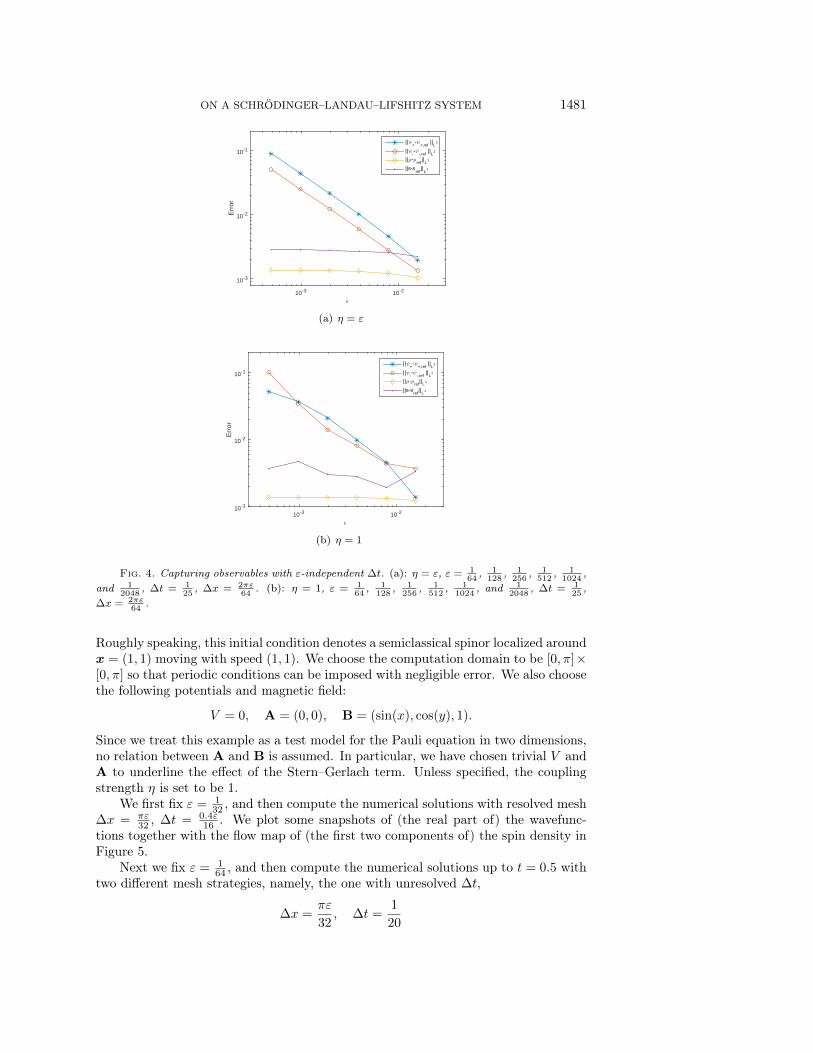
The errors in the wavefunctions, the position density, and the spin density are shownin Figure 4, from which we see clearly that the errors in the wavefunctions increaseas ε → 0, while the errors in the position density and the spin density stay almostunchanged. We then repeat the test for the coupling strength η = 1, and we observethe same tendency. Therefore, we have numerically verified that the TSSP methodwith unresolved time steps can give correct physical observables. It is worth empha-sizing that the analysis for this property is open when η = 1, so the tests here canonly serve as numerical evidence.

Example 4.2. In this example, we demonstrate the accuracy of the TSSP methodapplied to the Pauli equation in two dimensions. We choose the following WKB-typeinitial condition:

ψ+(x1, x2, 0) = ψ−(x1, x2, 0)

= exp

(ix1 − 1

ε

)exp

(ix2 − 1

ε

)exp

(− (x1 − 1)

2+ (x2 − 1)2

2ε

).

ON A SCHRÖDINGER–LANDAU–LIFSHITZ SYSTEM 1481

ǫ

10-3 10-2

Err

or

10-3

10-2

10-1

||ψ+-ψ

+,ref ||

L2

||ψ--ψ

-,ref ||

L2

||ρ-ρref

||L

1

||s-sref

||L

1

(a) η = ε

ǫ

10-3 10-2

Err

or

10-3

10-2

10-1

||ψ+-ψ

+,ref ||

L2

||ψ--ψ

-,ref ||

L2

||ρ-ρref

||L

1

||s-sref

||L

1

(b) η = 1

Fig. 4. Capturing observables with ε-independent ∆t. (a): η = ε, ε = 164, 1

128, 1

256, 1

512, 1

1024,

and 12048

, ∆t = 125, ∆x = 2πε

64. (b): η = 1, ε = 1

64, 1

128, 1

256, 1

512, 1

1024, and 1

2048, ∆t = 1

25,

∆x = 2πε64

.

Roughly speaking, this initial condition denotes a semiclassical spinor localized aroundx = (1, 1) moving with speed (1, 1). We choose the computation domain to be [0, π]×[0, π] so that periodic conditions can be imposed with negligible error. We also choosethe following potentials and magnetic field:

V = 0, A = (0, 0), B = (sin(x), cos(y), 1).

Since we treat this example as a test model for the Pauli equation in two dimensions,no relation between A and B is assumed. In particular, we have chosen trivial V andA to underline the effect of the Stern–Gerlach term. Unless specified, the couplingstrength η is set to be 1.

We first fix ε = 132 , and then compute the numerical solutions with resolved mesh

∆x = πε32 , ∆t = 0.4ε

16 . We plot some snapshots of (the real part of) the wavefunc-tions together with the flow map of (the first two components of) the spin density inFigure 5.

Next we fix ε = 164 , and then compute the numerical solutions up to t = 0.5 with

two different mesh strategies, namely, the one with unresolved ∆t,

∆x =πε

32, ∆t =

1

20

1482 JINGRUN CHEN, JIAN-GUO LIU, AND ZHENNAN ZHOU

ψ+ ( t=0.2)

x0.8 1 1.2 1.4 1.6 1.8 2

y

0.8

1

1.2

1.4

1.6

1.8

2

ψ+ ( t=0.3)

x0.8 1 1.2 1.4 1.6 1.8 2

y

0.8

1

1.2

1.4

1.6

1.8

2

ψ+ ( t=0.4)

x0.8 1 1.2 1.4 1.6 1.8 2

y

0.8

1

1.2

1.4

1.6

1.8

2

ψ- ( t=0.2)

x0.8 1 1.2 1.4 1.6 1.8 2

y

0.8

1

1.2

1.4

1.6

1.8

2

ψ- ( t=0.3)

x0.8 1 1.2 1.4 1.6 1.8 2

y

0.8

1

1.2

1.4

1.6

1.8

2

ψ- ( t=0.4)

x0.8 1 1.2 1.4 1.6 1.8 2

y

0.8

1

1.2

1.4

1.6

1.8

2

Fig. 5. Snapshots of (the real part of) the wavefunctions together with the flow map of (thefirst two components of) the spin density. ε = 1

32, ∆x = πε

32, ∆t = 0.4ε

16. Top Row: ψ+ for t = 0.2,

0.3, and 0.4. Bottom Row: ψ− for t = 0.2, 0.3, and 0.4.

and the one with resolved ∆t,

∆x =πε

32, ∆t =

0.5ε

16,

which gives the reference solutions. We plot the position density of each wavefunctionwith the flow map of (the first two components of) the spin density in Figure 6,from which we see obviously great agreement. Hence, we have again verified thatε-independent time steps can be used to calculate correct physical observables.

4.2. The Schrödinger–Landau–Lifshitz system. In this section, we test theTSSP method for the Schrödinger equation and the Gauss–Seidel projection methodfor the Landau–Lifshitz equation to understand spin and magnetization dynamicsunder different coupling regimes. For simplicity, we only consider one-dimensionalspace. Since the exact solution is not available in this case, we have ascertained thatthe results below are unchanged by refining both the spatial meshes and the time steps.

Example 4.3 (Weak coupling). Set Ω = [0, 1]. The external potential V (x) is setto be

√ε

x(x−1) so that the electron is confined in Ω. The final time t = 20. ∆t =

1/512, ε = 1/256, h = 1/512, ∆x = h/8, and α = 0.1. The coupling constantη = 0.01, which means the spin-magnetization coupling is weak. Initial conditionsfor the wavefunctions and magnetization are

ψ+ = ψ− =5√π

exp

(i0.1x

ε

)exp (−50(x− 0.5)2)

andm0(x) = (cos(x), sin(x), 0),

respectively.After the initial relaxation, the magnetization achieves its stable configuration,

which is (almost) a constant field with the third component almost 0 (Figure 7(a)).

ON A SCHRÖDINGER–LANDAU–LIFSHITZ SYSTEM 1483

ρ+ ( t=0.5)

x1 1.1 1.2 1.3 1.4 1.5 1.6 1.7 1.8 1.9 2

y

1

1.1

1.2

1.3

1.4

1.5

1.6

1.7

1.8

1.9

2

ρ- ( t=0.5)

x1 1.1 1.2 1.3 1.4 1.5 1.6 1.7 1.8 1.9 2

y

1

1.1

1.2

1.3

1.4

1.5

1.6

1.7

1.8

1.9

2

ρ+ ( t=0.5)

x1 1.1 1.2 1.3 1.4 1.5 1.6 1.7 1.8 1.9 2

y

1

1.1

1.2

1.3

1.4

1.5

1.6

1.7

1.8

1.9

2

ρ- ( t=0.5)

x1 1.1 1.2 1.3 1.4 1.5 1.6 1.7 1.8 1.9 2

y

1

1.1

1.2

1.3

1.4

1.5

1.6

1.7

1.8

1.9

2

Fig. 6. Comparison of the positition density of each wavefunction with the flow map of (thefirst two components of) the spin density. Top row: Solutions with unresolved ∆t. Bottom row:Solutions with resolved ∆t.

The real parts of the spin-up and spin-down wavefunctions at t = 20 are plottedin Figure 7(b). We also observe that the spin swings in a certain direction after theinitial relaxation. To get this direction, we calculate the angle between the spin whereits maximum magnitude is achieved and the magnetization is at the same position;see Figure 8(a). At t = 20, we plot the magnetization and spin directions in Figure8(b) and their projections along the x axis in Figure 8(c). The angle swings around28. Since the magnetization achieves its stable state at later times, the spin swingsaround 28 with respect to the magnetization.

In this case, η = 0.01 is small and the magnetization has a stable configuration,which is not affected by spin dynamics. This is consistent with the rigorous result ofthe semiclassical limit of (1) and (2) in the weak coupling regime [5].

Set the final time t = 10000. The long-time dynamics is shown in Figure 9. Againan (almost) periodic swing is observed for spin dynamics. The angle between spinand magnetization, where the maximum magnitude of spin is achieved, is around 0.However, the spin shows a complicated configuration and is not just simply alignedwith the magnetization.

Example 4.4 (Strong coupling). Set Ω = [0, 1]. The external potential V (x) is setto be

√ε

x(x−1) so that the electron is confined in Ω. The final time t = 20. ∆t = 1/512,

1484 JINGRUN CHEN, JIAN-GUO LIU, AND ZHENNAN ZHOU

0 0.2 0.4 0.6 0.8 1−1

−0.5

0

0.5

1

x

m(x

)

m1

m2

m3

(a) Magnetization

0 0.2 0.4 0.6 0.8 1−4

−3

−2

−1

0

1

2

3

4

x

Reψ

(x)

Reψ1

Reψ2

(b) Wavefunction

Fig. 7. Configurations of magnetization and the real part of the wavefunctions at t = 20 whenη = 0.01. (a): Magnetization. (b): Wavefunction.

0 5 10 15 2026.5

27

27.5

28

28.5

29

29.5

30

30.5

t

θ(t)

(de

gree

)

(a) Angle

00.5

11.5

0

0.02

0.04

0.06−0.02

0

0.02

0.04

0.06

xy

z

SpinMagnetization

(b) Direction

00.010.020.030.040.050.06−0.01

0

0.01

0.02

0.03

0.04

0.05

0.06

y

z

SpinMagnetization

(c) Projection

Fig. 8. Spin-magnetization angle in terms of time, arrow plot of spin and magnetization inthree dimensions, and their projections along the x axis at t = 20. An (almost) periodic swing isobserved for spin dynamics when η = 0.01. (a): Angle. (b): Direction. (c): Projection.

0 2000 4000 6000 8000 100000

5

10

15

20

25

30

35

t

θ(t)

(de

gree

)

(a) Angle0

0.51

1.5

−0.05

0

0.05

0.1−4

−2

0

2

4x 10

−3

xy

z

SpinMagnetization

(b) Direction−0.0200.020.040.060.08

−3

−2

−1

0

1

2

3x 10

−3

y

z

SpinMagnetization

(c) Projection

Fig. 9. Spin-magnetization angle in terms of time, arrow plot of spin and magnetization inthree dimensions, and their projections along the x axis at t = 10000. An (almost) periodic swingwith the angle 0 is observed for spin dynamics when η = 0.01 if time is long enough. The spin isnot just simply aligned with the magnetization. (a): Angle. (b): Direction. (c): Projection.

ε = 1/256, h = 1/512, ∆x = h/8, and α = 0.1. The coupling constant η = 10,which means the spin-magnetization coupling is strong. Initial conditions for thewavefunctions and magnetization are

ψ+ = ψ− =5√π

exp

(i0.1x

ε

)exp (−50(x− 0.5)2)

andm0(x) = (cos(x), sin(x), 0),

respectively.

ON A SCHRÖDINGER–LANDAU–LIFSHITZ SYSTEM 1485

0 0.2 0.4 0.6 0.8 1−1

−0.5

0

0.5

1

x

m(x

)

m1

m2

m3

(a) Magnetization

0 0.2 0.4 0.6 0.8 1−2

−1

0

1

2

3

4

5

x

Reψ

(x)

Reψ1

Reψ2

(b) Wavefunction

Fig. 10. Configurations of magnetization and the real part of wavefunctions at t = 20 whenη = 10. (a): Magnetization; (b): Wavefunction.

0 5 10 15 200

5

10

15

20

25

30

t

θ(t)

(de

gree

)

(a) Angle

00.5

11.5

−0.05

0

0.05

0.1−5

0

5

10x 10

−4

xy

z

SpinMagnetization

(b) Direction

−0.0200.020.040.06−2

0

2

4

6

8

10x 10

−4

y

z

SpinMagnetization

(c) Projection

Fig. 11. Spin-magnetization angle in terms of time, arrow plot of spin and magnetization inthree dimensions, and their projections along the x axis at t = 20. An (almost) periodic swing isobserved for spin dynamics when η = 10. (a): Angle. (b): Direction. (c): Projection.

After the initial relaxation, the magnetization achieves its stable configuration,which is (almost) a constant field (Figure 10(a)). The real parts of the spin-up andspin-down wavefunctions at t = 20 are plotted in Figure 10(b). We calculate the anglebetween the spin where its maximum magnitude is achieved and the magnetizationis at the same position; see Figure 11(c). The angle drops to 0 quickly and a perfectalignment between spin and magnetization is observed. This is consistent with thephysical intuition [17].

5. Conclusion and perspectives. In this paper, we have made two majorcontributions. We have established a dynamical model for the spin density and themagnetization coupling phenomenon from a variational perspective and constructed ahybrid numerical method for the Schrödinger–Landau–Lifshitz system, where the timesplitting spectral method for the quantum wavefunction has been rigorously analyzed.In accordance with our simulations, in the weak coupling regime, η = O(ε), themagnetization configuration first evolves to a stable configuration, and the interactionbetween the spin density and the magnetization is not manifestly noticeable untilt = O( 1

ε ). However, in the strong coupling regime, η = O(1), the magnetizationand the spin density reach their respective stable configurations within O(1) time,where the angle between the principal direction of the spin density and that of themagnetization is approaching zero, which demonstrates the alignment phenomenon.

In the future, we may explore the existence and asymptotic behavior of the solu-tions to the Schrödinger–Landau–Lifshitz system and design better numerical methodsfor the Landau–Lifshitz equation.

1486 JINGRUN CHEN, JIAN-GUO LIU, AND ZHENNAN ZHOU

Acknowledgments. J. Chen, J. Liu, and Z. Zhou would like to thank HaroldU. Baranger and Lihui Chai for helpful discussions.

REFERENCES

[1] M. N. Baibich, J. M. Broto, A. Fert, F. N. Van Dau, F. Petroff, P. Etienne,G. Creuzet, A. Friederich, and J. Chazelas, Giant magnetoresistance of(001)Fe/(001)Cr magnetic superlattices, Phys. Rev. Lett., 61 (1988), pp. 2472–2475,doi:10.1103/PhysRevLett.61.2472.

[2] W. Bao, S. Jin, and P. A. Markowich, Spectral approximations for the Schrodingerequation in the semi-classical regime, J. Comput. Phys., 175 (2002), pp. 487–524, doi:10.1006/jcph.2001.6956.

[3] A. Brataas, A. D. Kent, and H. Ohno, Current-induced torques in magnetic materials,Nat. Mater., 11 (2012), pp. 372–381, doi:10.1038/nmat3311.

[4] W. F. Brown Jr., Micromagnetics, Wiley, New York, 1963.[5] L. Chai, C. J. García-Cervera, and X. Yang, Semiclassical Limit of the Schrödinger-

Poisson-Landau-Lifshitz-Gilbert System, preprint, 2016.[6] J. Chen, C. J. García-Cervera, and X. Yang, Mean-field dynamics of the spin-

magnetization coupling in ferromagnetic materials: Application to current-driven domainwall motions, IEEE Trans. Magn., 51 (2015), pp. 1–6, doi:10.1109/TMAG.2015.2401534.

[7] J. Chen, C. J. García-Cervera, and X. Yang, A mean-field model of spin dynamicsin multilayered ferromagnetic media, Multiscale Model. Simul., 13 (2015), pp. 551–570,doi:10.1137/140953149.

[8] R. Cheng and Q. Niu, Microscopic derivation of spin-transfer torque in ferromagnets, Phys.Rev. B, 88 (2013), 024422, doi:10.1103/PhysRevB.88.024422.

[9] T. L. Gilbert, Phys. Rev., 100 (1955), p. 1243. [Abstract only; full report, Armor ResearchFoundation Project No. A059, Supplementary Report, May 1, 1956 (unpublished)].

[10] L. Greengard and J. Y. Lee, Accelerating the nonuniform fast Fourier transform, SIAMRev., 46 (2006), pp. 443–454, doi:10.1137/S003614450343200X.

[11] P. Grünberg, R. Schreiber, Y. Pang, M. B. Brodsky, and H. Sowers, Layered magneticstructures: Evidence for antiferromagnetic coupling of Fe layers across Cr interlayers,Phys. Rev. Lett., 57 (1986), pp. 2442–2445, doi:10.1103/PhysRevLett.57.2442.

[12] B. Guo and S. Ding, Landau–Lifshitz Equations, World Scientific, Singapore, 2008.[13] A. Hubert and R. Schäfer, Magnetic Domains: The Analysis of Magnetic Microstructures,

Springer, Berlin, 1998.[14] I. Žutić, J. Fabian, and S. Das Sarma, Spintronics: Fundamentals and applications, Rev.

Mod. Phys., 76 (2004), pp. 323–410, doi:10.1103/RevModPhys.76.323.[15] S. Jin, P. A. Markowich, and C. Sparber, Mathematical and computational methods for

semiclassical Schrödinger equations, Acta Numer., 20 (2011), pp. 121–209, doi:10.1017/S0962492911000031.

[16] S. Jin and Z. Zhou, A semi-Lagrangian time splitting method for the Schrödinger equationwith vector potentials, Commun. Inf. Syst., 13 (2013), pp. 247–289, doi:10.4310/CIS.2013.v13.n3.a1.

[17] J. I. Kaplan, Diffusion constant in the effective Bloch equation for ferromagnetic resonancein metals, Phys. Rev., 143 (1966), pp. 351–352, doi:10.1103/PhysRev.143.351.

[18] L. Landau and E. Lifshitz, On the theory of the dispersion of magnetic permeability inferromagnetic bodies, Physikalische Zeitschrift der Sowjetunion, 8 (1935), pp. 153–169.

[19] Z. Ma, Y. Zhang, and Z. Zhou, An improved semi-Lagrangian time splitting spectral methodfor the semi–classical Schrödinger equation with vector potentials using NUFFT, Appl.Numer. Math., 111 (2017), pp. 144–159.

[20] G. Panati, H. Spohn, and S. Teufel, Effective dynamics for Bloch electrons: Peierlssubstitution and beyond, Commun. Math. Phys., 242 (2003), pp. 547–578, doi:10.1007/s00220-003-0950-1.

[21] G. Panati, H. Spohn, and S. Teufel, Motions of electrons in adiabatically perturbed periodicstructures, Analysis, Modeling and Simulation of Multiscale Problems, Springer, Berlin,2006, pp. 595–617.

[22] Y. Qi and S. Zhang, Spin diffusion at finite electric and magnetic fields, Phys. Rev. B, 67(2003), 052407, doi:10.1103/PhysRevB.67.052407.

[23] D. C. Ralph and M. D. Stiles, Spin transfer torques, J. Magn. Magn. Mater., 320 (2008),pp. 1190–1216, doi:10.1016/j.jmmm.2007.12.019.

ON A SCHRÖDINGER–LANDAU–LIFSHITZ SYSTEM 1487

[24] X.-P. Wang, C. J. García-Cervera, and W. E, A Gauss–Seidel projection method formicromagnetics stimulations, J. Comput. Phys., 171 (2001), pp. 357–372, doi:10.1006/jcph.2001.6793.

[25] S. Zhang, P. M. Levy, and A. Fert, Mechanisms of spin-polarized current-driven magneti-zation switching, Phys. Rev. Lett., 88 (2002), 236601, doi:10.1103/PhysRevLett.88.236601.

[26] S. Zhang and Z. Li, Roles of nonequilibrium conduction electrons on the magnetizationdynamics of ferromagnets, Phys. Rev. Lett., 93 (2004), 127204, doi:10.1103/PhysRevLett.93.127204.