multiresolution schemes - home di homes.di.unimi.it · fondamenti di elaborazione del segnale...

Multiresolution schemesFondamenti di elaborazione del segnale multi-dimensionale

Multi-dimensional signal processing

Stefano Ferrari

Universita degli Studi di [email protected]

Elaborazione dei Segnali Multi-dimensionali e Applicazioni2014–2015

Motivations

I Transforms give an alternative view of a signal.

I The Fourier Transform of a signal f (x) gives a representationof the same signal in the frequency domain.

I The processing should reveal information not directlyaccessible from the signal.

I The Fourier Transform gives information on the presence offrequency components.

I It is impossible to localize them.I It can be critical for non-stationary signals.

I Wavelets perform what is called space-frequencyrepresentation:

I information on the frequency components,I localized in space.

.

Stefano Ferrari— Multi-dimensional signal processing— a.a. 2014/15 1

Motivations (2)

I Besides wavelet transform allows to describe the image atdifferent resolutions:

I features detection at different scales;I selective denoising;I compression and transmission.

I Multiresolution representation allows to perform linear filteringoperations using the same (small) filter for each resolution,instead of using larger filter for coping with large features inthe full resolution image.

Multiscale representation

I The concepts from which the wavelet transform can bederived root in several disciplines.

I In particular for images, multiscale representations have beenproposed before the wavelets.

I Among them, at least the following have to be mentioned:I Gaussian pyramidI Laplacian pyramidI Scale spacesI Subband coding

.


Scale

Operating at different scales is a concept exploited in severalapproaches.

I Features are not independent of image scale:I their actual size depends on the resolution of the image and

the distance from the camera.

I For example, Marr-Hildreth edge detector:

1. filter with a Gaussian of a suitable scale;2. compute the Laplacian;3. find the zero-crossing.

I Also the Canny edge detector makes use of Gaussiansmoothing.

I The size of the smoothing filter has to increase with the scaleparameter.

Multiscale representation

Multiscale (or multigrid) representation are based on a simpleobservation:

I fine scales need high resolution,

I for coarse scales, low resolution copies.

Hence a M-levels multigrid representation of an image, f , can beobtained as:

I f0 = f

I fm+1 = S↓2[fm], n = 0, . . . , M − 1

where S↓2[·] is a suitable downsampling operator.

I Note: ↓ 2 means that one sample out of two in each directionis discarded;

I other downsampling rates are theoretically possible, but notuseful in practice.

.


Multiscale representation (2)

I Multigrid representation does not increase too much thestorage requirements:

I given N2 the number of pixel of f0,I N2/4 are required for f1,I N2/16 for f2,I N2/2m for fm.I Less than 4

3 N2 pixels are required.

I Since S↓2[·] operates on the previous level, the total numberof operations for obtaining the whole multigrid representationis proportional to 4

3 N2.

I Multigrid are also known as pyramidal representations (Burtand Adelson, 1983).

Multiscale representation (3)

.


Downsampling operator

Naive choices for S↓2[·] may produce undesirable effects.

I S↓2[·] =↓ 2 may produce aliasing.I Smoothing is required.

I Smoothing cancels high frequency variations that may causealiasing when downsampled.

I Gaussian is generally chosen as smoothing operator.I Multigrid representation are called Gaussian pyramid.

I Smoothing and downsampling allow small filters or smallspatial operators to operate on large scale features.

Upsampling operator

Some operations require the recovering of the original size of thelower levels of the pyramid.

I It happens when different levels content has to be compared.

I This operation is carried out by the upsampling operator,R↑2[·]

I A suitable rule for estimating the missing pixels is required.I Generally, every even pixel of each row is estimated from the

odds;I then, the same procedure is applied considering the column

direction.

.


Laplacian pyramid

A complementary representation can be derived from the Gaussianpyramid:

I lm = fm − R↑2[fm+1]

I lM−1 = fM−1

where M is the number of pyramid levels.

This representation is called Laplacian pyramid.I It provides a bandpass decomposition of the image.

I lm contains those components belonging to fm, but not in fm−1.I lM−1 contains the low frequencies components (coarsest scale

structures).

Laplacian pyramid (2)

From a Laplacian pyramid, the original image can be recursivelyreconstructed.

I The scheme for computing the Laplacian pyramid can beinverted:

I lM−1 = fM−1

I fm−1 = lm−1 + R↑2[fm]

I Errors in the computation of lm−1 due to R↑2[·] are absorbedin the reconstruction.

.


Laplacian pyramid (3)

Since Laplacian images histograms are usually more dense in asmall neighborhood of zero, compression algorithms can performbetter on Laplacian pyramids than on Gaussian ones.

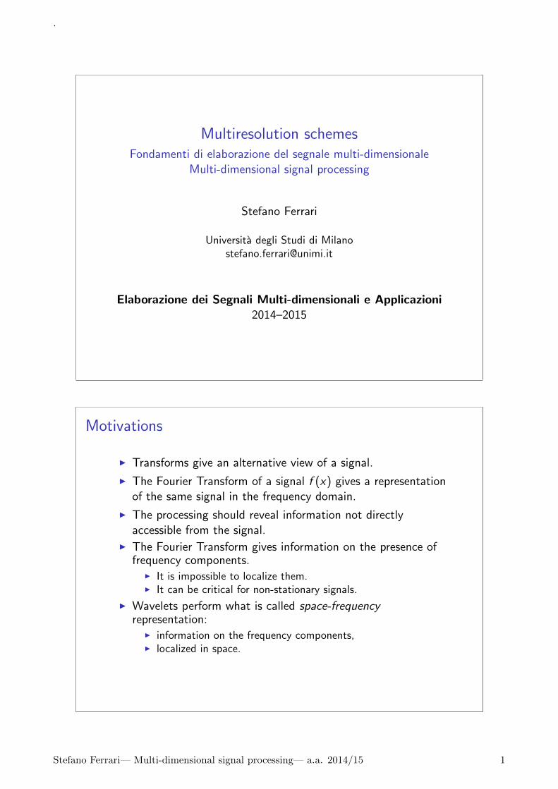
Pyramid scheme

.


Pyramid example

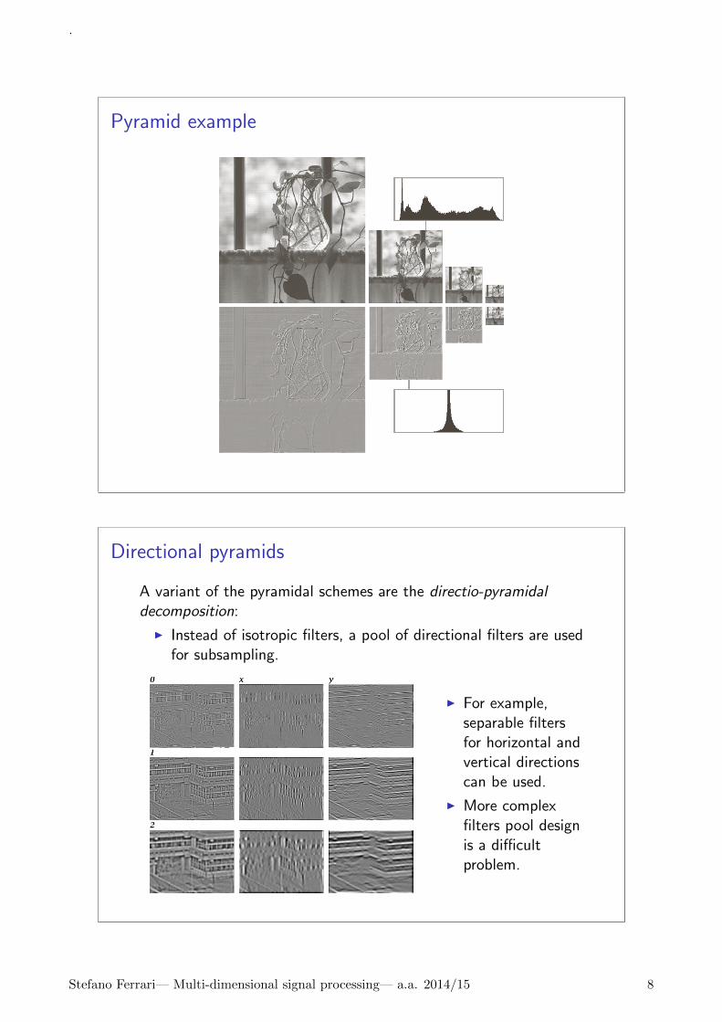
Directional pyramids

A variant of the pyramidal schemes are the directio-pyramidaldecomposition:

I Instead of isotropic filters, a pool of directional filters are usedfor subsampling.

I For example,separable filtersfor horizontal andvertical directionscan be used.

I More complexfilters pool designis a difficultproblem.

.


Scale spaces

I Pyramidal representation allows for a very rigid multiscaleprocessing.

I The scale parameter can vary only of a factor of two betweeneach level.

I Scale space scheme allows a continuous changing of the scaleparameter.

I The scale space is generated by blurring the image at a givendegree.

I This can be modelled as a diffusion process (such as heat).I Spatial concentration differences in the gray level are equalized.I The scale is modelled as the time and the diffusion process

produces the scale space.

I It can be shown that for an homogeneous diffusion process,the version of the image f at the scale t, ft , can be computedas the convolution of f with a Gaussian of variance t.

Scale spaces (2)

a edges andpoints

b periodicpattern

c random

d small andlargefeatures

.


Scale spaces (3)

a f0 = f

b f1

c f4

d f16

Scale spaces (4)

A scale space filter must ensure two important properties to thegenerated scale space.

1. No new details have to be added as the scale parameterincreases.

I The image information content must decrease with the scaleparameter.

I It can be formalized with the maximum-minimum principle:I local extrema cannot be enhanced.

2. The scale space does not depend on the scale parameter fromwhich the diffusion starts.

I Scale invariance principle.I Starting with an image at the scale t1 and applying the

smoothing operator at scale t2, the image at scale t1 + t2 isobtained.

Gaussian kernel is the only convolution kernel isotropic andhomogeneous that meet these two properties.

.


Scale spaces (5)

a Gaussian diffusion b Box diffusion

I In b, nor maximum-minimum principle, neither scale invariance(structures that disappear and appear again later) hold.

I In a, the smoothing progress as the square of the time: thetime needed to blur a detail is proportional to the square of itssize.

I A non linear scale coordinate is produced.

Scale spaces (6)

Several variants stem from these schema.

I Quadratic and exponential increasing scale parameter;I accelerated diffusion process.

I Differential (Laplacian) scale spaces;I the change of the image with the scale is explicited.

I Discrete scale spaces;I the diffusion process is discretized.

.


Subband coding

I Subband coding operates on the frequency domain.

I The image is decomposed in bandlimited components, calledsubbands.

I The decomposition is invertible:I from the subbands, the original image can be recovered.

I The decomposition is realized by means of FIR digital filters.I FIR stands for Finite Impulse Response.

Digital filtering

I Digital filtering is formalized by the convolution of the inputsignal, f (·), composed of discrete samples, with the filter, h(·)composed of a finite number, K , of samples:

f (n) =∞∑

k=−∞h(k) ∗ f (n − k)

where filter values out of [0, K − 1] are zero.

I When the impulse is input, the filter coefficients are output:

h(n) =∞∑

k=−∞h(k) ∗ δ(n − k)

.


Subband coding and decoding

I Each module (coding/decoding) is composed of a filter banks,each containing two filters.

I In a filter banks, the signal is passed through all the filters.I ↓ 2 is the downsampling operator, which discard the odd index

samples;I ↑ 2 is the upsampling operator, which insert a 0 valued sample

after each sample.

Subband coding and decoding (2)

I The analysis filter bank decomposes the input sequence f (n)in two (half length) subsequences, fl and fh.

I The filter h0 is a lowpass filter, while h1 is a highpass filter: fl

and fh have a content in different frequency interval: thesubbands.

I fl is called an approximation of f .I fh is the detail of f .

.


Subband coding and decoding (3)

I The synthesis filter bank recombines the subbandsubsequences, fl and fh, to produce the sequence f .

I The two sequences, fl and fh, are upsampled and filteredthrough the filters g0 and g1 respectively, and then summed.

I If h0, h1, g0, and g1 are such that f = f , they are calledperfect reconstruction filters.

Filter design

I In order to achieve the perfect reconstruction filters, the filtersmust be related in two ways:

g0(n) = (−1)nh1(n)

g1(n) = (−1)n+1h0(n)

or g0(n) = (−1)n+1h1(n)

g1(n) = (−1)nh0(n)

I The filters are cross modulatedI g0 ↔ h1 and g1 ↔ h0

I and are biorthogonal:

〈hi (2n − k), gj(k)〉 = δ(i − j)δ(n), i , j = {0, 1}

.


Filter design (2)

I If they enjoy the following property:

〈gi (n), gj(n + 2m)〉 = δ(i − j)δ(n), i , j = {0, 1}

the filter banks are orthonormal.

I Orthonormal filters, for even K , satisfy:

g1(n) = (−1)ng0(K − 1− n)

hi (n) = gi (K − 1− n), i = {0, 1}

I Orthonormal filter banks are defined from only one of itsfilters (prototype).

Image subband coding

I 1D orthogonal and biorthogonal filter banks can be used alsofor image (2D) processing.

I Considering 1D filtering as a separable transform, rows andcolumns can be processed in sequence.

I Four subimages areobtained:

I a(m, n),approximation

I dV (m, n),vertical detail

I dH(m, n),horizontal detail

I dD(m, n),diagonal detail

.


Image subband coding (2)

I The schema canbe iteratively usedfor obtaining amultiresolutionrepresentation.

Wavelets definition

I The wavelets, ψa, b(·), are scaled and translated copies of thesame function, ψ:

ψa,b(x) =1√|a|

ψ

(x − b

a

)a, b ∈ R, a > 0

I The function ψ(·) that generates the wavelet is called motherwavelet.

I The parameter a is the scale parameter.I It describes the length of space window embraced by ψa, b.

I The parameter b is the shift parameter.I It describes the position of the window along the space-line.

.


Continuous Wavelet Transform

I The Continuous Wavelet Transform (CWT) is defined as:

W (a, b) = 〈f , ψa,b〉 =∞∫−∞

f (x)ψ?a,b(x) dx

= 1√|a|

∞∫−∞

f (x)ψ?(x−ba

)dx

I The amplitude of W (a, b) measures the similarity between fand ψa,b.

I In this sense, the CWT analyzes f (·).

Space-frequency window

I The Fourier transform of ψa,b(x) is:

F(ψ) = ψa,b(ν) =a√|a|

e−ινb ψ(aν)

I ψa,b(·) embraces large intervals for small values of a, shortintervals for large values of a

I W (a, b) can be reframed as (Parseval):

2πW (a, b) =⟨

f , ψ⟩

I It can be shown that CWT has:I high frequency resolution and low space resolution for high

values of aI low frequency resolution and high space resolution for small

values of a

.


Space-frequency window (2)

I Hence:I a is large ⇒ CWT gives fine information on the FT of x , but

poor localization in space;I a is small ⇒ CWT gives very local information in space, but

very general in frequency.

I Very useful property for real cases:I short events has only high frequency components;I long events are characterized by low frequencies.

Invertibility

I Invertibility is a desirable property for a signal transform.

I It can be shown that if

Cψ =

∫ ∞

−∞

|ψ(ν)|2ν

dν <∞

the CWT W (a, b) is invertible:

f (x) =1

Cψ

∫ ∞

−∞

∫ ∞

−∞W (a, b)ψa,b(x)

da db

2

I Hence, it is possible to reconstruct f (·) from the coefficientsof its CWT, W (a, b).

I This operation is often called synthesis.

.


Why wavelets?

I From Cψ <∞, it can be derived that ψ(0) = 0.

I Hence, ψ(·) must oscillate.I It can be also shown that ψ(·) ∈ L2(R);

I f ∈ L2 ⇔ ||f || =√∫

t∈R f 2(x) dx <∞I ψ have some limitations in space and frequency.

I The term wavelet (small wave) derives from these conditions;I ondina in Italian, ondelette in French.

Morlet wavelet

−5 −4 −3 −2 −1 0 1 2 3 4 5−1

−0.8

−0.6

−0.4

−0.2

0

0.2

0.4

0.6

0.8

1Morlet wavelet

0 2 4 6 8 100

0.5

1

1.5

2

2.5

3FT Morlet wavelet

(a) (b)

The Morlet wavelet (a), and its Fourier transform (b).It is a planar wave localized by a Gaussian.

ψ(x) = eι5xe−x2

2σ

.


Haar wavelet

−0.5 0 0.5 1 1.5

−1

−0.8

−0.6

−0.4

−0.2

0

0.2

0.4

0.6

0.8

1

Haar wavelet

−100 −80 −60 −40 −20 0 20 40 60 80 1000

0.1

0.2

0.3

0.4

0.5

0.6

0.7

0.8FT Haar wavelet

(a) (b)

The Haar wavelet (a), and its Fourier transform (b).

ψ(x) =

1 0 ≤ x < 1/2−1 1/2 ≤ x ≤ 1

0 otherwise

Shannon wavelet

−5 −4 −3 −2 −1 0 1 2 3 4 5−1

−0.8

−0.6

−0.4

−0.2

0

0.2

0.4

0.6

0.8

1

Shannon wavelet

−10 −8 −6 −4 −2 0 2 4 6 8 10

0

0.2

0.4

0.6

0.8

1

FT Shannon wavelet

(a) (b)

The Shannon (or sinc) wavelet (a), and its Fourier transform (b).It is a family parametrized by νb (bandwidth) and νc (centerfrequency).

ψ(x) =√νb sinc(νbx) e2ιπνcx

.


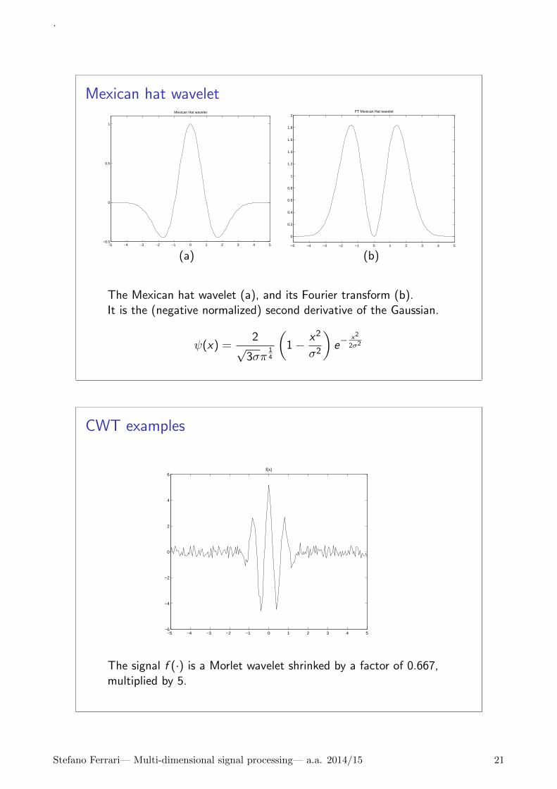
Mexican hat wavelet

−5 −4 −3 −2 −1 0 1 2 3 4 5−0.5

0

0.5

1

Mexican Hat wavelet

−5 −4 −3 −2 −1 0 1 2 3 4 5

0

0.2

0.4

0.6

0.8

1

1.2

1.4

1.6

1.8

2FT Mexican Hat wavelet

(a) (b)

The Mexican hat wavelet (a), and its Fourier transform (b).It is the (negative normalized) second derivative of the Gaussian.

ψ(x) =2

√3σπ

14

(1− x2

σ2

)e−

x2

2σ2

CWT examples

−5 −4 −3 −2 −1 0 1 2 3 4 5−6

−4

−2

0

2

4

6f(x)

The signal f (·) is a Morlet wavelet shrinked by a factor of 0.667,multiplied by 5.

.


CWT examples: Morlet wavelet

−5 −4 −3 −2 −1 0 1 2 3 4 5−6

−4

−2

0

2

4

6f(x)

−5 −4 −3 −2 −1 0 1 2 3 4 5−1

−0.8

−0.6

−0.4

−0.2

0

0.2

0.4

0.6

0.8

1Morlet wavelet

Morlet Wavelet Transform

−5 −4 −3 −2 −1 0 1 2 3 4 5

0.5

1

1.5

2

2.5

3

50

100

150

200

250

CWT examples: Haar wavelet

−5 −4 −3 −2 −1 0 1 2 3 4 5−6

−4

−2

0

2

4

6f(x)

−0.5 0 0.5 1 1.5

−1

−0.8

−0.6

−0.4

−0.2

0

0.2

0.4

0.6

0.8

1

Haar wavelet

Haar Wavelet Transform

−1 −0.5 0 0.5 1 1.5 2

0.5

1

1.5

2

2.5

3

50

100

150

200

250

.


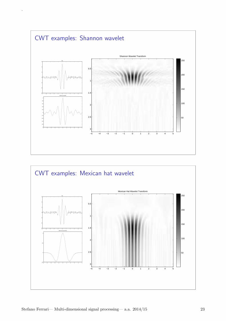
CWT examples: Shannon wavelet

−5 −4 −3 −2 −1 0 1 2 3 4 5−6

−4

−2

0

2

4

6f(x)

−5 −4 −3 −2 −1 0 1 2 3 4 5−1

−0.8

−0.6

−0.4

−0.2

0

0.2

0.4

0.6

0.8

1

Shannon wavelet

Shannon Wavelet Transform

−5 −4 −3 −2 −1 0 1 2 3 4 5

0.5

1

1.5

2

2.5

3

50

100

150

200

250

CWT examples: Mexican hat wavelet

−5 −4 −3 −2 −1 0 1 2 3 4 5−6

−4

−2

0

2

4

6f(x)

−5 −4 −3 −2 −1 0 1 2 3 4 5−0.5

0

0.5

1

Mexican Hat wavelet

Mexican Hat Wavelet Transform

−5 −4 −3 −2 −1 0 1 2 3 4 5

0.5

1

1.5

2

2.5

3

50

100

150

200

250

.


Space-frequency locality

The quantities x , ∆x , ν, ∆ν

x =1

||ψ(x)||2∫ ∞

−∞x |ψ(x)|2 dx

∆2x =

1

||ψ(x)||2∫ ∞

−∞(x − x)2 |ψ(x)|2 dx

ν =1

||ψ(ν)||2∫ ∞

−∞ν |ψ(ν)|2 dν

∆2ν =

1

||ψ(ν)||2∫ ∞

−∞(ν − ν)2 |ψ(ν)|2 dν

characterize the wavelet’s distribution in the space and frequencydomains.

Space-frequency locality (2)

I In fact, ν is the center of mass of the wavelet in the spacedomain, and the energy of ψ is concentrated in a 2∆x longneighborhood of x .

I Same considerations hold for ν and ∆ν with respect to ψ.

I Applying the above defined quantities to ψa,b, it can be shownthat ψa,b is concentrated around b + ax with radius a∆x ,

while ψ is concentrated around νa with radius ∆ν

a .

I Hence, the region

[b + ax − a∆x , b + ax + a∆x ]×[ν −∆ν

a,ν + ∆ν

a

]

is where the wavelet ψa,b lives in the space-frequency domain.

.



I The region

[b + ax − a∆x , b + ax + a∆x ]×[ν −∆ν

a,ν + ∆ν

a

]

is called the space-frequency window of the wavelet.I Actually, as usually ν = 0 and ˆψ(0) = 0, the wavelet is

localized in symmetric disjointed bands, such as[−ν2

a , −ν1

a ] ∪ [ν1

a ,ν2

a ].

I The shape of the window, 2a∆x × 2 ∆xa , depends on a.

I Its position in space depends also on b.

I The window area is constant: 4∆x∆ν .I As it can be shown that ||ψ(x)||2 ≤ 2||x ψ(x)|| ||ν ψ(ν)||

(Heisenberg), the window size has a lower bound;I although it can depend upon the actual wavelet.


I Since the coefficients of the CWT W (a, b) reflect thesimilarity of the signal f and ψa,b, they describe the behaviorof the signal in the wavelet window.

I For a > 1, the wavelet is dilated, and its frequency contentmove toward lower frequencies.

I The opposite for a < 1 (the wavelet is shrinked).I Hence, fast events can be captured by wavelets with a small

a:I the window base is 2a∆x wide, good localization in space

I and long events can be described by wavelet with large a:I the window height is ∆ν

a , good frequency resolution.

.


Discrete representation of the CWT

I The CWT W (a, b) can be represented as an image I (i , j):Morlet Wavelet Transform

−5 −4 −3 −2 −1 0 1 2 3 4 5

0.5

1

1.5

2

2.5

3

50

100

150

200

250

I i represents a given scale, a(i);

I j represents a given position, b(j);

I the color in I (i , j) is proportional tothe value (modulus or phase) of thecoefficient W (a(i), b(j)).

I This operation is a discretization of the CWT.I The parameters a and b are discretized.I It is not the Discrete Wavelet Transform.I It is just a sampling of W (a, b).

I How choosing a(i) and b(j)?I Do not loose critical information.I Can the signal f (x) be obtained from the {W (a(i), b(j))}

sampling?

Dyadic sampling

I To be able to reconstruct a signal from its sampling, thesampling frequency have to be at least double of the maximumfrequency component of the signal (Nyquist’s theorem).

I The frequency content of X (a, b) diminishes when a increases.

I Hence, the sampling frequency can be different for differentscales.

I This allows to save computational resources.I Usually, sampling on the dyadic grid:

I logarithmic law for scales: a = 2−j , j ∈ Z;I translations proportional to scales: b = ka, k ∈ Z;I the logarithmic law allows to cover a wide range of scales with

a relatively small number of scales (and samples).

I In general, sparser the sampling, more restrictions on thewavelet.

.


Short-time Fourier Transform (STFT)

I The Short-time (or Short-term) Fourier Transform (STFT) isdefined as:

STFT (f (x)) = W (τ, ν) =

∫ ∞

−∞f (x)w(x − τ)e−ινx dx

I It is the FT of a signal windowed by the function w(·), whileit slid along the space.

I The function w(·) can be a Gaussian with a given width, σ.I This is the case of the Gabor transform.

I The STFT realizes a space-frequency transform.I How STFT compares with CWT?

Space-frequency coverage

I Sampling vs. FT space-frequency coverage:

space

freq

uen

cy

sampling

space

freq

uen

cy

FT

.


Space-frequency coverage (2)

I STFT space-frequency coverage:

I CWT space-frequency coverage:

Mathematical view of the signal transforms

I Signals can be seen as functions (real, complex).I Usually a subset of the functions can be considered.

I E.g., the continuous function (up to the n-th order), C n, orthe L2 functions (finite energy).

I These sets are (infinite dimensional) vector spaces.

I The transform describes the signal as a linear combination ofother functions (the basis vectors).

I Hence, the transformed signal is constituted of the coefficientsof the linear combination.

I I.e., the “importance” of each basis function for describing thesignal.

.


Mathematical view of the signal transforms (2)

I The basis functions declared in the transforms limit the subsetof the representable functions:

I the vector space generated by the basis;I setting to zero some coefficients (e.g., for noise suppression)

means considering only a subset of the vector space.

I Some other issues:I The decomposition always exists?

I Which properties must have the signal to be transformed?

I Is the decomposition unique?I Different coefficients can reconstruct the same signal?

Inner product

I The inner product, 〈·, ·〉, on the vector space V is a functionV × V → R such that, for each v1, v2 ∈ V and α ∈ R:

I 〈v1, v1〉 ≥ 0, with 〈v1, v1〉 = 0 iif v1 = 0;I 〈v1, v2〉 = 〈v2, v1〉;I 〈αv1, v2〉 = 〈v1, αv2〉 = α〈v1, v2〉

I An inner product induces the norm, || · ||: ||v1|| =√〈v1, v1〉

I Two vectors v1 and v2 are orthogonal if 〈v1, v2〉 = 0.

I A basis {vk | vk ∈ V } is orthogonal if the vectors areorthogonal each others.

I A basis {vk | vk ∈ V } is orthonormal if the vectors areorthogonal each others and have a unitary norm:

〈vk , vj〉 = δk−j =

{1, k = j0, k 6= j

.


Bases

I If {vk | vk ∈ V } is an orthonormal basis, every vector v ∈ Vcan be expressed as:

v =∑

k

〈v , vk〉vk

I Two bases {vk | vk ∈ V } and {wk |wk ∈ V } are biorthogonalif:

〈vk ,wj〉 = δk−j =

{1, k = j0, k 6= j

In this case, the following relations hold:

∀v ∈ V v =∑

k

〈v ,wk〉vk and v =∑

k

〈v , vk〉wk

Back to the functions

I The inner product of the functions f and g , f , g ∈ L2(R) is:

〈f , g〉 =

∫ ∞

−∞f (x)g∗(x) dx

I It represents the projection of a signal onto the other.

I Hence, the FT of a signal and its inverse can be seen as adecomposition in terms of basis composed of sinusoidal andcosinusoidal functions.

I Same apply for CWT and its inverse.

.


multiresolution schemes - home di homes.di.unimi.it · fondamenti di elaborazione del segnale...

Documents