multiprocessor global scheduling on frame-based … global scheduling on frame-based dvfs systems...

HAL Id: inria-00442004https://hal.inria.fr/inria-00442004

Submitted on 17 Dec 2009

HAL is a multi-disciplinary open accessarchive for the deposit and dissemination of sci-entific research documents, whether they are pub-lished or not. The documents may come fromteaching and research institutions in France orabroad, or from public or private research centers.

L’archive ouverte pluridisciplinaire HAL, estdestinée au dépôt et à la diffusion de documentsscientifiques de niveau recherche, publiés ou non,émanant des établissements d’enseignement et derecherche français ou étrangers, des laboratoirespublics ou privés.

Multiprocessor Global Scheduling on Frame-BasedDVFS Systems

Vandy Berten, Joël Goossens

To cite this version:Vandy Berten, Joël Goossens. Multiprocessor Global Scheduling on Frame-Based DVFS Systems.Laurent George and Maryline Chetto andMikael Sjodin. 17th International Conference on Real-Timeand Network Systems, Oct 2009, Paris, France. pp.169-178, 2009. <inria-00442004>

https://hal.inria.fr/inria-00442004

https://hal.archives-ouvertes.fr

Multiprocessor Global Scheduling on Frame-Based DVFS Systems

Vandy BERTENUniversite Libre de Bruxelles

Fonds National de la Recherche [email protected]

Joel GOOSSENSUniversite Libre de Bruxelles

[email protected]

Abstract

In this work, we are interested in multiprocessor energyefficient systems where task durations are not known inadvance but are known stochastically. More precisely weconsider global scheduling algorithms for frame-basedmultiprocessor stochastic DVFS (Dynamic Voltage andFrequency Scaling) systems. Moreover we consider pro-cessors with a discrete set of available frequencies.

We provide a global scheduling algorithm, and for-mally show that no deadline will ever be missed. Fur-thermore, we present simulations showing that we havean energy benefit in doing global scheduling instead ofstatic partitioning.

1 Introduction

Nowadays, it is straightforward that energy efficiencyis a crucial aspect of embedded systems where a hugenumber of small and very specialized autonomous de-vices are interacting together through many kinds of me-dia (wired/wireless network, bluetooth, GSM/GPRS, in-frared. . . ). Moreover, we know that the uniprocessorparadigm will no longer hold in those devices. Even today,a lot of mobile phones are already equipped with severalprocessors.

In this work, we are interested in multiprocessor en-ergy efficient systems, where task durations are not knownin advance, but are known stochastically, which meansthat we know the probabilistic distribution of their exe-cution time. More precisely, we consider global schedul-ing algorithms for frame-based multiprocessor stochas-tic DVFS (Dynamic Voltage and Frequency Scaling) sys-tems. Moreover, we consider processors with a discreteset of available frequencies.

In the past few years, a lot of work has been providedin multiprocessor energy efficient systems. Most workwas done considering static partitioning strategies, mean-ing that a task was assigned to a specific processor, andeach instance of this task runs on the same processor. Firstof those work were devoted to deterministic tasks (with atask duration known beforehand, or the worst-case is con-sidered), such as [1, 10, 4, 5], and later probabilistic mod-

els were also considered [8, 7]. Only a little work has beenprovided about global scheduling, such as [3], but for de-terministic systems, or [11], using some slack reclamationmechanism, but not really using stochastic information.

As far as we know, no work has been provided withglobal scheduling on stochastic tasks. We propose to worktowards this direction. Notice that the frame-based modelwe consider in our work, where all tasks share the same(synchronous) period or deadline, is also used by manyresearchers, such as [10, 3, 7, 11]. This model attracts alot of attention, both from industry and theoretical com-munity. In the current state of the art of stochastic low-power multiprocessor systems, the knowledge we haveabout very general models is not accurate enough to allowpractical implementations. This is why simple but realisticmodels are interesting, but can be seen as a step towardsmore general models which are going to be considered ina near future.

The contribution of this paper is to provide a first algo-rithm allowing to efficiently schedule a frame-based taskset on a multiprocessor DVFS platform. We will proofthat our algorithm never misses deadlines, and will showhow we can save energy, compared to partitioned systems.

The paper is organized as follows: we first present thetask and system model we consider. Secondly we presentour algorithm, and prove its correctness. Then we pro-vide some simulation results attesting the benefit of doingglobal scheduling, and finally we conclude and give someperspectives.

2 Model

We consider a set of n non parallel and non preemptivetasks τ = {τ1, . . . , τn}. Task τi requires x cycles with aprobability ci(x), and its maximum number of cycles iswi(Worst Case Execution Cycles, or WCEC). The numberof cycles a task requires is not known before the end ofits execution. We consider a frame-based model, whereall tasks share the same (synchronous) period or deadlineD. In the following, D denotes the frame length, and aswe manage each frame independently, we denote by t = 0the beginning of each frame.

Those tasks run on m identical CPUs Π1, . . . ,Πm, andeach of those CPUs can run at M frequencies f1, . . . , fM .

In Proc. of the 17th International Conference on Real-Time and Network SystemsRTNS'2009, Paris, ECE, 26-27 October, 2009

In this work, the execution time is assumed to be strictlyproportional to the CPU frequency: if task τi takes α unitsof time at frequency fk, the same task would have taken

αfkf`

at frequency f`.

We consider that tasks cannot be preempted, but differ-ent instances of the same task can run on different proces-sors, i.e., task migrations are allowed, but job migrationsare not. We are interested in global scheduling techniqueswhich schedule a queue of tasks; each time a CPU is avail-able, it picks up the first task in the queue, choose a fre-quency, and run the job. We assume the system is workconserving1, and the job order has been chosen before-hand, but in some cases, in order to ensure the schedula-bility, the scheduler can adapt that order. In other words,we assume that the initial task order is not crucial and canbe considered to be a soft constraint. We will discuss laterin this work the importance of the task order.

2.1 ExamplesA simple example where this kind of system can be

useful is a system where n web-cams are connected toa device with m processors. If the web-cams are syn-chronous, they could all send an image, let say, 24 timesa second, and all those images should be processed beforethe next arrival. Task τi consists then in processing theimages of the ith web-cam, which can be done on any ofthe m processors.

A symmetric example can also be considered: am−CPUs device receives a stream containing, 24 times asecond, n compressed images to decompress, and to sendto n screens. In both cases, we know the distribution ofthe processing time, and would like to reduce as much aspossible the energy consumed by the processors.

3 Global Scheduling Algorithm

In [2], we have provided techniques allowing to sched-ule such a task set on a single CPU. The main idea is tocompute (offline) a function giving, for each task, the fre-quency to run the task based on the time elapsed in thecurrent frame. This function, Si(t) gave the frequencyat which τi should run if started at time t in the currentframe. Here, for the sake of clarity, we are going to con-

sider the symmetric function of S: Si(d)def= Si(D − d)

gives the frequency for τi if this task is started d units oftime before the end of the frame.

In the uniprocessor case, we were able to give schedu-lability guarantees, as well as good energy consumptionperformance, using the worst case number of cycles, aswell as the probability distribution of the number of cy-cles. We want to be able to provide both in this multipro-cessor case, using a global scheduling algorithm. As faras we know, global scheduling algorithm on multiproces-

1A work conserving system is a system where tasks never wait inten-tionally. In other words, if a task is ready, no processor can be idle.

sor system using stochastic tasks, and a limited number ofavailable frequencies, has not been considered so far.

The idea of our scheduling algorithm is to consider thata system with m CPUs, and a frame length D, is “close”to a system with a single CPU, but a frame length m×D,or, with a frame length D, but m times faster. We thenfirst compute a set of n S-functions considering the sameset of tasks, but a deadline m×D. A very naive approachwould consist in considering that when a task ends at timet, the total remaining available time before the deadline isthe sum of remaining time available on each CPU, whichmeans D − t on the current CPU, and D − tp on the otherones, where at each instant, tp represents the worst timeat which the task currently running on Πp will end, or thecurrent time if no task is running. Then, we could useSi(d) to choose the frequency.

Unfortunately, this simple approach does not work, be-cause a single task cannot use time on several CPUs simul-taneously, i.e., task parallelism is forbidden. However, ifthe number of tasks is reasonably greater than the num-ber of CPUs, we think that in most cases, Si(d) will notrequire to use more than the available time on the currentCPU, and somehow, will let the available time on otherCPUs for future tasks. And when Si(d) requires more timethan actually available, we just use a faster frequency.

Of course, we need to ensure the schedulability of thesystem, which cannot be guaranteed with the previous ap-proach: for instance, at the end of a frame, we might havesome slack time unusable because too short to run any ofthe remaining tasks. But as this time has been taken intoaccount when we chose the frequency of previous tasks,we might miss the deadline if we do not take any precau-tion.

The algorithm we propose is composed of two phases,an off-line phase, and an on-line one. The off-line oneconsists in performing a (virtual) static partitioning, aim-ing at reserving enough time in the system for each task.This phase is close to what we did in [2] using the con-cept of Danger Zones. Briefly, in uniprocessor systems,the danger zone of a task τi starts at zi, where zi is suchthat if this task is not started immediately, we cannot en-sure that this task and every subsequent tasks can all befinished by the deadline. In other words, if a task starts inits danger zone, and this task and all the subsequent onesuse their WCEC, even at the highest frequency, some taskswill miss the (common) deadline.

The on-line phase uses both this pre-reservation to en-sure the schedulability (but performing dynamic changesto this static partitioning), and the S-functions, to improvethe energy efficiency.

3.1 Virtual Static PartitioningThis first phase, which is performed offline, aims at

“virtually” assigning each task to one processor — virtu-ally meaning that a task assigned to a processor does notnecessarily run on that processor — in such a way that ifeach task assigned to one processor takes its worst case


execution number of cycles, we can still manage to finishthose tasks in a frame of length D. Figure 1, left part,shows an example of such a partitioning.

This basic idea is to put those tasks on the right sideof the schedule (in light grey on Figure 1), just before thedeadline, with the amount of time they would need to runin the worst case at the highest frequency. We call thisgrey zone the reservation zone. When we start a task, weremove it from this reservation zone, and start it, but in away that a task that we run will never overlap with a taskreservation even in the worst case.

The partitioning problem boils down to have n objectsof size wi

fM,∀i ∈ {1, . . . , n} that we need to put in m

boxes of lengthD. This is actually a bin packing problem,and the optimal algorithm (giving a valid partitioning forevery partitionable system) is known to be NP-hard [6].

If we denote by Γp the set of tasks assigned to CPU Πp,we need to find an assignment such as:∑

τq∈Γp

wqfM≤ D ∀p ∈ {1, . . . ,m},

meaning that no CPU has more than what it could run inthe worst case, and

∀p 6= q,Γp ∩ Γq = ∅

meaning that a task cannot be assigned to several proces-sors, ⋃

p

Γp = τ

which means all the tasks are assigned to some processor.During the on-line phase, the partitioning will be up-

dated by moving some tasks from a processor to anotherone. As long as those tasks have not started yet, theycan be moved without any migration cost. But of course,a task can be moved to a processor Πp only if there isenough space between tp (the worst end of the task cur-rently running on this CPU), and D−Ap (the begin of thereservation zone, assuming the frame starts at time 0).

This static partitioning can be performed in manyways, but we propose in Algorithm 1 to do it as balancedas possible, by sorting tasks according to their WCEC.

Algorithm 1: Static partitioning

Ap = 0 ∀p ; // Reserved time on Πp

Γp = {} ∀p ; // Tasks assigned to Πp1

foreach τi descending sorted by wi do2

q = argminpAp; // CPU with the3

largest not yet assigned timeif D −Aq > wi

fMthen4

Aq = Aq + wi

fM; // τi reservation5

Γq = Γq ∪ τi ;6

else7

Failed!8

After this first step of virtual static partitioning, we cansee the system as in Figure 1, left part. Ap is the lengthof the reservation zone on Πp, then the length of the greypart.

Notice that it is not because we cannot manage to dothis virtual partitioning that the system is not schedulable.But at least, if we manage to do so, then we can ensurethat the system is schedulable, as we will show formallylater in this paper. This virtual static partitioning can becomputed offline, and used for the whole life of the sys-tem.

This partitioning can be done in O(n × logm), ifAp’s are stored in a heap. We also need in the off-linephase to compute the S-functions, which can be done inO(n2 ×M ×W ), where W is the number of samples inthe distribution, using for instance the PITDVSclosest algo-rithm described in [2].

Notice that the static partitioning aims at reservingthe minimum amount of time required in the worst case,then this amount of reserved time corresponds to the timeneeded to run the worst case at the highest frequency fM .Moreover, if the task number (written on tasks in Figure 1)gives the order in which tasks should be run, the parti-tioning is done sorting tasks on their worst case executiontime. So the order shown on the partitioning could seem tobe randomly chosen regarding to tasks number. However,tasks (virtually) assigned to a CPU can be seen as an un-ordered set: the only information we will need later aboutthis task set is its total size. And except in some specificcases, tasks will be picked up by increasing task number.

Figure 1 Left: Static partitioning. Right: State of thesystem after having started tasks {τ1, . . . , τ7}. Noticethat reservations (light grey tasks, right aligned) corre-spond to worst cases, while effective tasks (white tasks,left aligned) are actual execution times, and change thenfrom frame to frame. Vertical axis is frequency, horizontalis time. Then areas correspond to amount of computation.

4

5

7

12 36

10

12

911

8

0 D

∏1

∏2

∏3 3

712

10

9

11

8

0 D

1

2 4

5

6

t1 t3 t2

3.2 On-line AlgorithmBased on the virtual static partitioning, the main idea

of the on-line part is to start a task at a frequency whichallows it to end before the beginning of the reserved zoneon this processor. For instance, in Figure 1, τ1 could start


on Π1 using all the space between the beginning of theframe, and the reserved space for τ5. But we will see sit-uations where it would be more energy efficient to givemore time for τ1, in order to run it slower. In such cases,we can also move, for instance, τ5 or τ6 on Π2, or τ12 toΠ3. By doing so, and because we never let a running taskusing the reserved time of another (not started) task, wecan guarantee that, if we were able to build a partitioningin the off-line phase, no task will never miss its deadline.A formal proof of this will be given in Section 3.3. Ofcourse, as soon as a task starts, we release the reservedtime for this task.

The on-line part of the algorithm is given in Algo-rithm 4. We first give some explanation about two pro-cedures we need in the main algorithm.

Remark that as we only move tasks which have notstarted yet, we do not need to move any context or per-form any migration. The only thing we change is the in-formation that, in the future, a job is going to start on agiven processor.

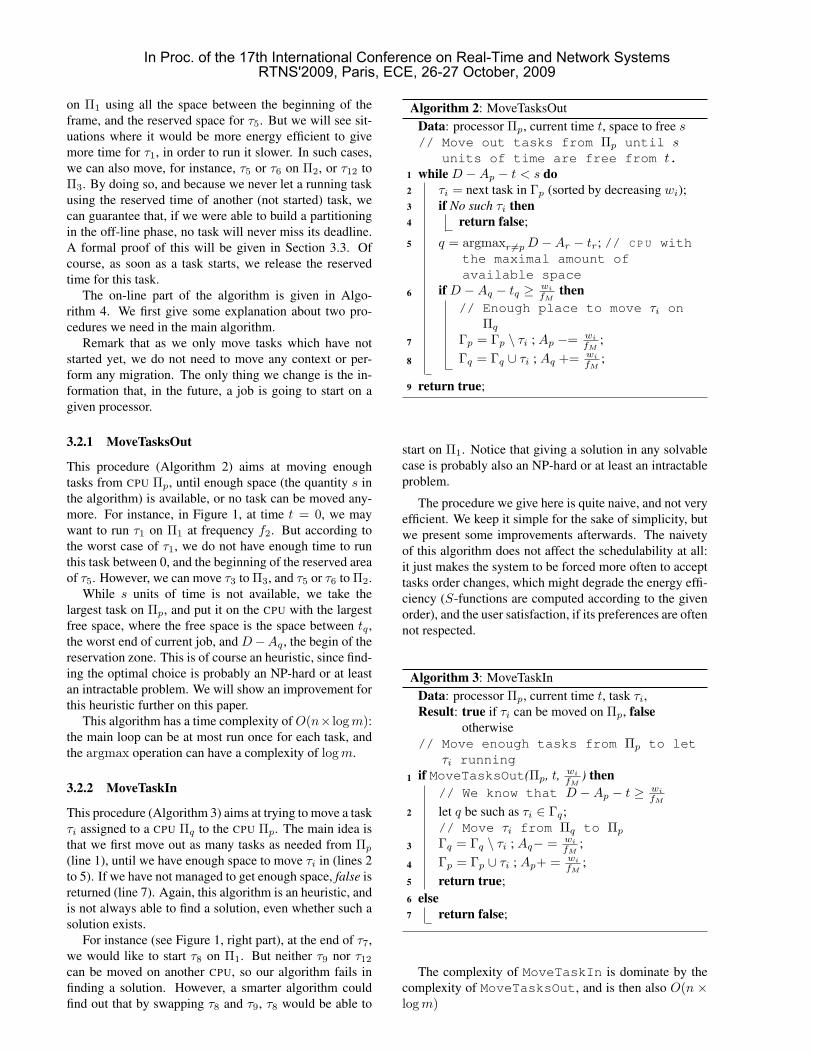
3.2.1 MoveTasksOut

This procedure (Algorithm 2) aims at moving enoughtasks from CPU Πp, until enough space (the quantity s inthe algorithm) is available, or no task can be moved any-more. For instance, in Figure 1, at time t = 0, we maywant to run τ1 on Π1 at frequency f2. But according tothe worst case of τ1, we do not have enough time to runthis task between 0, and the beginning of the reserved areaof τ5. However, we can move τ3 to Π3, and τ5 or τ6 to Π2.

While s units of time is not available, we take thelargest task on Πp, and put it on the CPU with the largestfree space, where the free space is the space between tq ,the worst end of current job, and D−Aq , the begin of thereservation zone. This is of course an heuristic, since find-ing the optimal choice is probably an NP-hard or at leastan intractable problem. We will show an improvement forthis heuristic further on this paper.

This algorithm has a time complexity ofO(n× logm):the main loop can be at most run once for each task, andthe argmax operation can have a complexity of logm.

3.2.2 MoveTaskIn

This procedure (Algorithm 3) aims at trying to move a taskτi assigned to a CPU Πq to the CPU Πp. The main idea isthat we first move out as many tasks as needed from Πp

(line 1), until we have enough space to move τi in (lines 2to 5). If we have not managed to get enough space, false isreturned (line 7). Again, this algorithm is an heuristic, andis not always able to find a solution, even whether such asolution exists.

For instance (see Figure 1, right part), at the end of τ7,we would like to start τ8 on Π1. But neither τ9 nor τ12

can be moved on another CPU, so our algorithm fails infinding a solution. However, a smarter algorithm couldfind out that by swapping τ8 and τ9, τ8 would be able to

Algorithm 2: MoveTasksOutData: processor Πp, current time t, space to free s// Move out tasks from Πp until s

units of time are free from t.while D −Ap − t < s do1

τi = next task in Γp (sorted by decreasing wi);2

if No such τi then3

return false;4

q = argmaxr 6=pD −Ar − tr; // CPU with5

the maximal amount ofavailable space

if D −Aq − tq ≥ wi

fMthen6

// Enough place to move τi onΠq

Γp = Γp \ τi ; Ap −= wi

fM;7

Γq = Γq ∪ τi ; Aq += wi

fM;8

return true;9

start on Π1. Notice that giving a solution in any solvablecase is probably also an NP-hard or at least an intractableproblem.

The procedure we give here is quite naive, and not veryefficient. We keep it simple for the sake of simplicity, butwe present some improvements afterwards. The naivetyof this algorithm does not affect the schedulability at all:it just makes the system to be forced more often to accepttasks order changes, which might degrade the energy effi-ciency (S-functions are computed according to the givenorder), and the user satisfaction, if its preferences are oftennot respected.

Algorithm 3: MoveTaskInData: processor Πp, current time t, task τi,Result: true if τi can be moved on Πp, false

otherwise// Move enough tasks from Πp to let

τi runningif MoveTasksOut(Πp, t, wi

fM) then1

// We know that D −Ap − t ≥ wi

fM

let q be such as τi ∈ Γq;2

// Move τi from Πq to Πp

Γq = Γq \ τi ; Aq− = wi

fM;3

Γp = Γp ∪ τi ; Ap+ = wi

fM;4

return true;5

else6

return false;7

The complexity of MoveTaskIn is dominate by thecomplexity of MoveTasksOut, and is then also O(n ×logm)


3.2.3 Main algorithm

Here are the main steps of the procedure given in Algo-rithm 4, which is called each time a CPU (say Πp) is avail-able, at time t, with τi the next task to start. This procedurewill always start a task at a speed guaranteeing deadlines,but not necessarily τi.

• line 1: We first evaluate d, the remaining time wehave for τi, . . . , τn: if tq is the worst time where Πq

is going to be available (the time of the last start, plusthe worst case execution time of the current task atthe chosen frequency), we have:

d = (D− t)+∑q 6=p

(D− tq) = mD−

t+∑q 6=p

tq

.

• line 2: Let f = Si(d), the frequency chosen for τi inthe single CPU model with d units of time before thedeadline. We are going to check if we can use thisfrequency (we assume this frequency to be a “good”one from the energy consumption point of view).

• line 3–6: If τi was not assigned to Πp, we first tryto move it to Πp (Algorithm 3). If we have enoughspace on Πp, the situation is easy. Otherwise, weneed to move some tasks out from Πp, in order tocreate enough space.

• line 5: If we cannot manage to make enough space,then we are not able to start τi right now. We try thenthe same procedure for τi+1, but we need to left-shiftS−functions of wi

fM. This is not required from the

schedulability point of view (we ensure the schedula-bility by controlling the available time), but we guessit will improve the energy consumption. For the samereason, we will need to right-shift functions of thesame amount when τi starts, because we have onetask less to run after τi.

This improvement is not presented here, but we haveimplemented it in the simulation we present in thispaper. It requires to be done carefully, because wemight have several swapped tasks.

• line 9: If we succeeded, we try to move as many tasksas possible from Πp to other CPUs (Algorithm 2), un-til we have enough space to start τi at f , or no taskcan be moved anymore. We then start τi either atf , or at the smallest frequency allowing to run τi inthe space we manage to free (line 10). As τi was as-signed to Πp (possibly after some changes), we areat least sure that we can start τi at fM .

Notice that when StartTask is invoked, it is alwayspossible to run a job, and therefore, we will never considerτn+1 in Algorithm 4, line 5 (see next section for a proof).

The complexity of StartTask is a little bit com-plex, because this function is recursive. Let first com-pute the complexity when we do not need to invoke

Algorithm 4: StartTaskData: Processor Πp, time t, task τid = m×D −

(t+∑q 6=p tq

); // Available1

time on the system

f = Si(d); // Freq. we want to run τi2

if τi /∈ Γp then3

// τi is not on Πp, we try tomove it in

if not MoveTaskIn(Πp, t, τi) then4

StartTask(Πp, t, τi+1);5

return;6

// We have now τi ∈ ΓpAp− = wi

fM; // Release τi reservation7

Γp = Γp \ τi;8

// Try to remove enough tasks (ifneeded) from Πp to allow τi torun at the desired speed f

if not MoveTasksOut(Πp, t, wi

f ) then9

// Not enough time to run τi at f// We know that D −Ap − t < wi

f

f =⌈

wiD −Ap − t

⌉F

;10

tp+ = wi

f ; // Worst end time for τi11

Start τi at f ;12

StartTask at line5. We have m (sum at line 1)+ log(m) (line 2) + n logm (MoveTaskIn at line 4)+ n logm (MoveTasksOut at line 9), then O(m +n logm).

If we do invoke StartTask recursively, then in theworst case, we have a depth of n calls. In this case, lines 1to 5 are run n times (O(n× (m+n logm)), and lines 7 to12 only once (O(n logm)). Then, in total (O(n × (m +n logm)).

3.3 CorrectnessIn this section, we will show the correctness of this al-

gorithm, meaning that the on-line algorithm does not jeop-ardize the schedulability provided by the off-line phase.We will need two proofs for this: first, we will show thatif we are able to obtain a virtual static partitioning, thenwe will always meet the deadline. Then, we will showthat the algorithm “StartTask” runs all the tasks.

We remind the reader that tq is the worst end time oftasks running on Πq . If no task is running on this CPU, tqis actual end time of the last task which ran on Πq , 0 if notask has ever started on this CPU.

We first provide a definition:

Definition 1. Let Aq the “reserved time” on Πq , i.e.∑p:τp∈Γq

wp

fM.

A correct state is a state where, on each CPU Πq , theworst end tq is always lower than the begin of the reserved


zone [D − Aq, D], or, more formally, a state is said to becorrect iff

tq ≤ D −Aq ∀q ∈ [1, . . . ,m].

We will show that, starting from a correct state, onestep of the algorithm StartTask (or one call to Algo-rithm 4) will reach another correct state.

Lemma 1. Algorithm 4 keeps states correct.

Proof. In order to show the lemma, we will prove that, ifbefore we call the algorithm, we have tq ≤ D − Aq,∀q,this condition is still respected at the end. We will denoteby A′q the value of Aq before we call the algorithm, andby A′′q this value after the call. We then have to show that

tq ≤ D −A′q ⇒ tq ≤ D −A′′q .

We first show that MoveTasksOut (Algorithm 2) andMoveTaskIn (Algorithm 3) respect this property.

MoveTasksOut (Algorithm 2, page 4). We can show thatany iteration of the while loop keeps the property. Theonly lines that change Aq are the line 7 and 8. Here, wedenote by A′q (resp. A′′q ) the value of Aq at the beginning(resp. the end) of the loop.

For Aq , we have from line 6 that D − A′q − tq ≥ wi

fM.

From line 8, we have A′′q = A′q + wi

fM. Then,

D −A′′q +wifM− tq ≥

wifM

,

and therefore, tq ≤ D −A′′q .ForAp, as we remove a task from Πp, the condition re-

mains obviously true. Remark that, if the function returnstrue, we can easily see that D −Ap − t ≥ s.

MoveTaskIn (Algorithm 3, page 4). The proof isvery similar to the previous one. We first callMoveTasksOut, which preserves the condition, as wehave shown above. And with the same way as before, wecan show that lines 3 and 4 also preserve the condition,because we run them if and only if D −Ap − t ≥ wi

fM.

StartTask (Algorithm 4, page 5). The first part of the al-gorithm (lines 1 to 6) preserves the condition tq ≤ D−Aqfor sure: lines 1 and 2 do not change any value in the con-dition, MoveTaskIn preserves the condition, and if weinvoke StartTask, we return right after the call.

When we are at line 7, we know that τi, the task wewant to start, is on Πp, the CPU which has just been re-leased, or τi ∈ Γp. As A′′p = A′p − wi

fM.

Notice that as t corresponds to the time at which Πp hasjust been released (or at the begin of the frame if t = 0),we have t = tp.

Line 7 preserves the property, because we reduce Ap(if tp ≤ D − Ap − wi

fM, then tp ≤ D − Ap), as well as

MoveTasksOut at line 9.

At line 9, we have two cases that we will con-sider separately. Notice that, as we stated before,MoveTaskIn(Πp, t,

wi

f ) returns true if and only if D −Ap − t ≥ wi

f . Then we can see the line 9 as the test‘if(D −Ap − t < wi

f )’.Let t′p be the value of tp just before the test. By hy-

pothesis, we know that t′p ≤ D−Ap (Ap does not changein this part).

If D−Ap− t′p ≥wif

, we have t′′p = t′p +wif

, and then

t′′p ≤ D −Ap, which validates the first case.

If D − Ap − t′p <wif

, then line 10 makes that f ≥wi

D −Ap − t, and then D − Ap − t′p ≥

wif

, and we can

then apply the same proof as above.We now have finished the proof: if tp ≤ D−Ap is true

before we call StartTask, this condition is still true atthe end of the procedure.

Remark that we do not need to make any hypothesis onSi(t), except that this function always return an allowedfrequency.

Lemma 2. All tasks are started by the algorithm.

Proof. The reason why we need to proof this is that wesometime skip a task, if we are not able to start it rightnow without violating any reservation.

We first have to do the hypothesis that StartTask isalways called with the task with the smallest index thathas not started yet. But of course, StartTask couldpossibly call recursively itself with a task with an higherindex.

We can consider separately three cases:

• The task τi is already allocated to CPU Πp. Then τican for sure start on Πp right away, possibly at thehighest speed;

• The task τi is not on CPU Πp, but we can move itthere. So we are in the same situation as the firstcase;

• The task τi is not on CPU Πp, and we cannot move itthere. We will now consider this last case.

If it is impossible to move τi on Πp, it is obviouslybecause there is at least one task already reserved on Πp.And as at the first level of StartTask, i is the smallestindex of the not started tasks, the reserved tasks have allan index larger than i. Let j be the smallest index of thetasks reserved on Πp.

As we cannot move τi on Πp, we call StartTaskwith τi+1. If i+ 1 = j or τi+1 can be moved on Πp, thenwe can start a task. Otherwise, we try with τi+2, τi+3, . . . ,and we are then sure to reach τj at some point, or to starta task with an index between i and j.

Theorem 1. If a virtual static partitioning can be found,then algorithm StartTask runs all jobs, and meets alldeadlines.


Proof. The proof is a direct consequence of the two pre-vious lemmas. The initial state, just after the virtual par-titioning has been performed, is correct: we have tq =0 ∀q ∈ [1, . . . ,m], and if the partitioning is correct, thenD ≤ Aq ∀q ∈ [1, . . . ,m].

We can also see that if the final state (when all task havefinished) is correct, then we have not missed any deadline:in the final state, Aq = 0 ∀q ∈ [1, . . . ,m]. Then, if thestate is correct, we have tq ≤ D ∀q ∈ [1, . . . ,m], wheretq is the end time of the last task running on Πq . And ob-viously, if all last tasks have finished before the deadline,no deadline has been missed.

As the initial state is correct, the algorithm preservesthe correctness, and all tasks are run by the algorithm, thenthe final state will be reach, and will be correct. Then alltasks meet their deadline.

3.4 Algorithm ImprovementA drawback of the algorithms we present here is that

in some cases, we are not able to start the task in thegiven order, and then accept to swap the order in whichtasks are started. But our S−functions are computed tobe efficient in the case we respect the order. Unfortu-nately, we have some cases where we cannot avoid intrin-sically this task swapping. But we can however improvethe function MoveTaskIn and MoveTasksOut in or-der the reduce the cases where we need to change the taskorder. We show here how to do that for MoveTaskIncan be improved, but a similar modification can be donefor MoveTasksOut.

The idea is that if we cannot manage to free enoughspace on the target CPU, then we can try to swap the taskwe want to move on this CPU with one of the task alreadythere.

Algorithm 5: Improvement for Algorithm 3(MoveTaskIn)

function CanSwap(τi, τj)p is such that τi ∈ Γp;q is such that τj ∈ Γq;

return(D − tp −

(Ap − wi

fM

)≥ wj

fM

and D − tq −(Aq − wj

fM

)≥ wifM

);

function SwapTasks(τi, τj)p is such that τi ∈ Γp;q is such that τj ∈ Γq;Γp = Γp \ τi ∪ τj ;Ap = Ap −

wifM

+wjfM

;

Γq = Γq \ τj ∪ τi;Aq = Aq −wjfM

+wifM

;

Those lines replace line 7 in Alg. 3 (MoveTaskIn):foreach j : τj ∈ Γp do

if CanSwap(τi, τj) thenSwapTasks(τi, τj);return true;

return false;

4 Simulation Results

In this section, we will present several simulations weperformed in order to evaluate the interest of doing globalscheduling of such frame-based multiprocessor platforms,in terms of energy savings. The simulator has been writ-ten in c++, by the authors of this paper. Before we reallyevaluate our scheduling algorithm, we will first study howthe task order can influence the gain in energy. We thencompare the energy consumed by a platform with staticpartitioning with the same platform and job characteris-tics, when global scheduling is allowed.

In the plots we present here, the load of a system (hori-zontal axis) is computed in this way: We first define Dmin

as the minimal deadline that any system can reach:

Dmin =m

fM

∑i

wi.

We then define the load of a system as the ratio betweenthe actual deadline D and the minimal deadline Dmin:

D

Dmin=

DfMm∑i wi

.

Of course, on multiprocessor systems, a load of 1 is veryrare to reach. A load of 10% does not mean that the systemis busy at 10%, but that, if we neglect switching times, andthe system only uses fM , it would be busy at 10%.

We have consider two task sets. For the first one, weconsider 32 tasks with normal distribution for the length(except that we truncate the tail in order to have a knownWCEC, and reject the negative values).

On another side, we consider real traces which havebeen collected in the National Taiwan University, CSIEdepartment, on devices decoding video streams. See [2]for more explanation about those traces. In the simulationwe present here, we have 18 such tasks for Figures 3, 6and 7, and 100 tasks for Figure 8.

In the following, we will mainly consider the Intel XS-cale CPU, but will also present some results on the IntelStrongArm SA-1100. The XScale provides 5 frequen-cies ranging from 150 to 1000 MHz, with a consumptiongoing from 80 mW at 150 MHz to 1.6 W at 1000 MHz.More details can be found for instance in [9]. The Stron-gArm has 11 frequencies, between 60 and 206 MHz.

4.1 Impact of the Task OrderIn this section, we compare several sorting criteria

defining different task orders. We did not conduct a fullstudy on this subject, and let this to further research, butwe wanted to see how simple criteria could impact on theperformance. We experimented many methods, but weonly present here a few of them (others did not show sig-nificant differences).

We evaluate several task characteristics in order to sorttasks. Here are the names given in the figures legend:

• rand: tasks are randomly ordered;


Figure 2

0.9

0.95

1

1.05

1.1

1.15

1.2

0.2 0.3 0.4 0.5 0.6 0.7 0.8 0.9

Ene

rgy

ratio

with

var

Load

32 Normally distributed tasks - 8 CPUs

randavg

wcec

Figure 3

0.95

1

1.05

1.1

1.15

1.2

1.25

1.3

1.35

1.4

1.45

1.5

0.2 0.3 0.4 0.5 0.6 0.7 0.8 0.9 1

Ene

rgy

ratio

with

var

Load

18 video decoding tasks - 4 CPUs

randavg

wcec

• wcec: tasks are sorted on decreasing worst case ex-ecution cycles;

• avg: tasks are sorted on decreasing average numberof cycles;

• var: tasks are sorted on decreasing variance.

Intuitively, we may think that tasks with a smaller vari-ance (or, in other words, with a better knowledge abouttheir execution time) should be put at the end of a frame.This way, the scheduler will have a better chance to fin-ish the last task very close to the deadline, and have thena slower average speed, which is known to be more effi-cient.

In Figures 2 (32 normally distributed (truncated) taskson 8 XScale) and 3 (18 tasks with realistic distribution,on 4 XScale), we show two systems, where we comparefor various loads the ratio between the energy consump-tion for var, and with the three other metrics. A valuehigher than one means then that, at that load, this metricconsumes more energy, and then performs worse.

At a first look, we can see that rand performs worsethat var on both platforms (using up to 15% more energyin the first plot, and up to 45% in the second case). Thetwo other metrics (var and avg) do not show significantdifference with the normal distribution (Fig. 2), but showa 10% loss in the realistic case, at high load.

The erratic aspect of the plots, especially the jumps wecan observe in Fig. 2 around 0.2, can be explained quitesimply, as we did for uniprocessor systems in [2]. Thespeed at which the first m tasks are started in a frame onlydepends upon the characteristics of the system, contraryto the speed of subsequent tasks, which will strongly de-pends on the time previous tasks actually took. Then, aslight change in the deadline, for instance, could causeone of the m first tasks to start at a higher speed, and hasthen a large impact on the system behavior.

4.2 Benefit of Globalization

Figure 4

0.85

0.9

0.95

1

1.05

1.1

1.15

1.2

1.25

0.2 0.3 0.4 0.5 0.6 0.7 0.8 0.9

Ben

efit

of g

loba

lizat

ion

Load


varrandwcec

avg

In the next few plots, we will try to see in which con-figuration we have any benefit in global scheduling. Asa first plot, we present in Figure 4 the same system as inFigure 2, but present another metric. Here, we show theratio between the energy consumed with static partition-ing and the energy with global scheduling. So the higher,the better is to use global scheduling. We show that forthe four sorting metrics we presented above.

In the first plot (Fig. 4 ; 32 normally distributed taskson 8 XScale CPUs), we can see that with rand, staticpartitioning performs better than global scheduling. Butfor other metrics, except at high load where it seemsto be quite unpredictable which strategy is better, globalscheduling saves always energy.

This plot does not show that static partitioning and ran-dom ordering is better that other strategies. It shows thatif the order is given and random, then we should not useglobal scheduling for this task set.

In order to better show how global scheduling performson this task set, we will show in Figure 5 the ratio be-tween all the combinations (a task ordering) and (global


or partitioning), and the global strategy on var. From thisfigure, we can see that any couple task ordering/strategybehaving better than var/global (meaning having most ofits point below 1) is also a global strategy.

Figure 5

0.9

0.95

1

1.05

1.1

1.15

1.2

1.25

0.2 0.3 0.4 0.5 0.6 0.7 0.8 0.9

Ene

rgy

ratio

with

var

(gl

obal

)

Load


rand (glob)avg (glob)

wcec (glob)var (part)

rand (part)avg (part)

wcec (part)

We also present here simulations with other system andtask parameters. Figure 6 presents the same system asin Figure 3 (but again with another metric). In Figure 7,we show the same task set, but on a StrongArm CPU. InFigure 8, we can see a much bigger system 100 (realistic)tasks, on a platform with 32 XScale CPUs.

All those simulations point out that when the order oftasks is arbitrary (e.g. rand), it sounds better to do staticpartitioning. But when the order is better, then most of thetime, we gain several percents of energy by doing globalscheduling. But not always for high loads: we observevery often that, for some high loads, static partitioningperforms better than global.

It could seem counter-intuitive that by being more rigid(i.e. static partitioning), we can be more efficient. Butseveral phenomena happen in our strategy, and can explainthis behavior.

First of all, in static partitioning system, when a taskends, we know exactly how much time we can give to thenext tasks allocated to the same CPU. This is the remain-ing time before the deadline. But in the global scheduling,we estimate the remaining time we will have for all taskswhich have not started yet. And we cannot be very ac-curate in this estimation, because when a tasks finishes,m − 1 tasks could be still running, and we do not knowwhen they will be over. We have then a less accurateknowledge about the system, which could lead to unluckydecisions.

Another phenomenon can be better understood by anexample. Let us imagine a system with 3 identical tasks(τ1, τ2 and τ3), and 2 CPUs (Π1 and Π2). If the variance isquite small, the scheduler on the equivalent uniprocessorsystem would choose to give each task approximately athird of the time space. On the dual processor system,the scheduler will then try to run τ1 up to 2D/3 on Π1,

and will make the same for τ2 on Π2. Then when thefirst of them ends, we have to start τ3, but we cannot use2D/3 units of time, because only half of this is availableon the released CPU, the other half being soon availableon the other one. And then we need to speed up the CPUon which τ3 runs, while the other CPU will be idle for athird of the frame length.

In the static partitioning case, we would have given allthe frame to one job on the first CPU, and would have splitthe frame into two equal parts on the second CPU. Andobviously, this scenario consumes less energy, because weuse a more constant frequency on one processor, and alower frequency on the other one.

Figure 6

0.8

0.85

0.9

0.95

1

1.05

1.1

1.15

1.2

0.2 0.3 0.4 0.5 0.6 0.7 0.8 0.9 1

Ben

efit

of g

loba

lizat

ion

Load


varrandwcec

avg

Figure 7

0.8

0.85

0.9

0.95

1

1.05

1.1

0.3 0.4 0.5 0.6 0.7 0.8 0.9 1

Ben

efit

of g

loba

lizat

ion

Load

18 video decoding tasks - 4 StrongArm CPUs

varrandwcec

avg

5 Conclusion and Future Work

In this paper, we have provided a first global schedulingalgorithm for multiprocessor stochastic low-power frame-based systems. We extended uniprocessor results, and weformally proved that, if a static partitioning can be found


Figure 8

0.8

0.85

0.9

0.95

1

1.05

1.1

1.15

1.2

0.1 0.2 0.3 0.4 0.5

Ben

efit

of g

loba

lizat

ion

Load


varrandwcec

avg

by any algorithm, then our scheduling algorithm will meetall deadlines.

Furthermore, we have shown through many simula-tions that this global algorithms can gain a lot of en-ergy compared to static methods, especially if the tasksare smartly ordered. We have shown several simulationswhere we can gain up to 20% by doing global schedulinginstead of static partitioning.

Lastly, our algorithm has a very reasonable on-line andoff-line complexity, and we strongly believe that it wouldbe easy to implement.

As a future work, here are a few points we want to lookdeeper, allowing to improve the energy consumption, orthe number of systems we are able to schedule.

• If we accept to change the frequency during the exe-cution of tasks, we can use the continuous model toobtain a frequency f , and use two frequencies dfeFand bfcF to “emulate” this f , where dfeF (resp.bfcF ) stands for the smallest frequency above (resp.largest below) f .

• Several steps require to solve NP-hard problemsby using some heuristics: Static partitioning (Al-gorithm 1), MoveTaskIn (Algorithm 3), andMoveTasksOut (Algorithm 2). The efficiency ofthe first one improves the number of systems we canaccept to schedule, the second one, the number oftasks we will need to swap (not run in the right or-der), and the third one, how close we can stay fromthe uniprocessor algorithm. We may try to furtherimprove those three algorithms.

• In order to reduce leakage or static energy consump-tion, we could turn off CPUs if they are not neededanymore before the end of the frame.

• We believe that if jobs are parallelizable, we can stillgain more energy by splitting them on several CPUs.But only a few research has been done on this subjectso far, and we think it is worth to be deeper studied.

References

[1] AYDIN, H., AND YANG, Q. Energy-aware partitioningfor multiprocessor real-time systems. In IPDPS’03: Pro-ceedings of the 17th International Symposium on Paral-lel and Distributed Processing (Washington, DC, USA,2003), IEEE Computer Society, p. 113b.

[2] BERTEN, V., CHANG, C.-J., AND KUO, T.-W. Dis-crete frequency selection of frame-based stochastic real-time tasks. In Proceedings of the 14th IEEE InternationalConference on Embedded and Real-Time Computing Sys-tems and Applications (Kaohsiung, Taiwan, August 2008),RTCSA2008, IEEE Computer Society, pp. 269–278.

[3] CHEN, J.-J., HSU, H.-R., CHUANG, K.-H., YANG, C.-L., PANG, A.-C., AND KUO, T.-W. Multiprocessorenergy-efficient scheduling with task migration consider-ations. In ECRTS’04: Proceedings of the 16th EuromicroConference on Real-Time Systems (Washington, DC, USA,2004), IEEE Computer Society, pp. 101–108.

[4] CHEN, J.-J., AND KUO, T.-W. Energy-efficient schedul-ing of periodic real-time tasks over homogeneous multi-processors. In PARC (September 2005), pp. 30–35.

[5] CHEN, J.-J., AND KUO, T.-W. Multiprocessor energy-efficient scheduling for real-time tasks with different powercharacteristics. In ICPP’05: Proceedings of the 2005 Inter-national Conference on Parallel Processing (Washington,DC, USA, 2005), IEEE Computer Society, pp. 13–20.

[6] GAREY, M. R., AND JOHNSON, D. S. Computersand Intractability : A Guide to the Theory of NP-Completeness (Series of Books in the Mathematical Sci-ences). W. H. Freeman, January 1979.

[7] MISHRA, R., RASTOGI, N., ZHU, D., MOSSE, D., AND

MELHEM, R. Energy aware scheduling for distributedreal-time systems. In IPDPS’03: Proceedings of the 17thInternational Symposium on Parallel and Distributed Pro-cessing (Washington, DC, USA, 2003), IEEE ComputerSociety, p. 21b.

[8] XIAN, C., LU, Y.-H., AND LI, Z. Energy-aware schedul-ing for real-time multiprocessor systems with uncertaintask execution time. In DAC ’07: Proceedings of the 44thannual conference on Design automation (New York, NY,USA, 2007), ACM, pp. 664–669.

[9] XU, R., MELHEM, R., AND MOSSE, D. A unified prac-tical approach to stochastic DVS scheduling. In EM-SOFT’07: Proceedings of the 7th ACM & IEEE interna-tional conference on Embedded software (New York, NY,USA, 2007), ACM, pp. 37–46.

[10] YANG, C.-Y., CHEN, J.-J., AND KUO, T.-W. An approxi-mation algorithm for energy-efficient scheduling on a chipmultiprocessor. In DATE’05: Proceedings of the confer-ence on Design, Automation and Test in Europe (Washing-ton, DC, USA, 2005), IEEE Computer Society, pp. 468–473.

[11] ZHU, D., MELHEM, R., AND CHILDERS, B. Schedulingwith dynamic voltage/speed adjustment using slack recla-mation in multi-processor real-time systems. In RTSS’01:Proceedings of the 22nd IEEE Real-Time Systems Sym-posium (RTSS’01) (Washington, DC, USA, 2001), IEEEComputer Society, pp. 686–700.


multiprocessor global scheduling on frame-based … global scheduling on frame-based dvfs systems...

Documents