multiple stable solutions for two-and...
TRANSCRIPT

96
Engineering e-Transaction (ISSN 1823-6379)
Vol. 7, No.2, December 2012, pp 96-106
Online at http://ejum.fsktm.um.edu.my
Received 16 Oct, 2012; Accepted 20 Dec, 2012
MULTIPLE STABLE SOLUTIONS FOR TWO-AND FOUR-SIDED LID-DRIVEN CAVITY FLOWS USING
FAS MULTIGRID METHOD
D.S. Kumara, A.K. Dass
a and A. Dewan
b
aDepartment of Mechanical Engineering, Indian Institute of Technology Guwahati,
Guwahati - 781039, India bDepartment of Applied Mechanics, Indian Institute of Technology Delhi
New Delhi - 110016, India
Email: [email protected]
ABSTRACT
The present work is concerned with the computations
of two- and four-sided lid-driven square cavity flows
to obtain multiple steady solutions using a time-
efficient FAS multigrid code based on the SIMPLE
algorithm on a colocated grid arrangement. The
transport equations are discretized using the QUICK
scheme for the convective terms and central-difference
scheme for the viscous and the pressure gradient terms.
The code is first validated against existing results for a
single-sided lid-driven square cavity flow. It is then
applied to the two- and four-sided lid-driven cavity
flows that involve multiple stable solutions. In the two-
sided square cavity two of the adjacent walls move
with an equal velocity and in the four-sided cavity all
the four walls move in such a way that parallel walls
move in the opposite directions with the same velocity.
The resulting flow fields show that a symmetric
solution exists for all Reynolds numbers whereas
multiplicity of states of one symmetric and two
asymmetric solutions for the two- and four-sided
cavity flows are identified above the critical Reynolds
number. The strategy employed to obtain these
solutions is described. For the first time a multigrid
strategy is employed to capture multiple steady states.
Keywords: Incompressible flows; lid-driven cavity;
finite-volume method; multiple solution; multigrid
method.
1.0 INTRODUCTION
In the past two decades the Semi Implicit Method for
Pressure Linked Equation (SIMPLE) algorithm is
probably the most widely used method for the
calculation of incompressible flows. The SIMPLE
algorithm of Patankar and Spalding (1972) is used to
couple the momentum and continuity equations. In this
method, the discretized equations for velocity
components and a pressure correction equation are
solved in a sequential manner. The pressure correction
formulation which is used to link the pressure and the
velocity fields, however, is weak and leads to slow
convergence or even divergence if appropriate under-
relaxations are not used. A major factor affecting the
performance of a scheme is its ability to smoothen out
the errors of all frequencies effectively in the solution.
Iterative methods, such as line-by-line solvers, provide
excellent smoothening of the errors of wavelengths
comparable to the mesh size. As the grid is refined,
these solvers show fast convergence in the initial few
iterations, but subsequently the convergence rate
deteriorates rapidly. This is due to the persistence of
low-frequency errors that are not effectively
smoothened by the repeated relaxation sweeps on a
given grid.
The multigrid methods exploit the ability of relaxation
procedures to efficiently smoothen the errors of
wavelengths comparable to the mesh size, by
employing a hierarchy of grids. By solving the
equations at different grid levels, the errors of all
frequencies are smoothened. The multilevel principle
can be used to accelerate the convergence of the
sequential as well as the coupled procedures. However,
the ability of the coupled procedures to implicitly
retain the velocity-pressure coupling makes the
multilevel application to the coupled solvers quite
attractive. Fedorenko (1962, 1964) is the originator of
the idea of multigrid which initially did not draw much
attention. Interest in the technique was reawakened
later by Brandt (1977). He also gave it a sound
mathematical foundation in a path-breaking paper in
1977. He was the first to demonstrate the practical
efficiency and generality of the multigrid methods. The
multigrid method was discovered independently by
Hackbusch (1978) at about the same time, who laid
firm mathematical foundations and provided reliable

97
methods. Multigrid methods have been analysed,
applied and generalized in many ways since their
introduction, and are gradually becoming recognized
as a powerful tool in applied mathematics.
Sivaloganathan and Shaw (1988) applied multigrid
method to SIMPLE pressure correction technique of
Patankar and Spalding using staggered grid. They
adopted the full-approximation storage multigrid
method and achieved a large reduction in CPU time.
Since then application of multigrid method in SIMPLE
pressure correction smoothers has increased.
Grid-coarsening process is difficult in staggered grid
arrangement because of the use of three different set of
cells. Hence a colocated grid layout is used in the
present work. The momentum interpolation proposed
by Rhie and Chow (1983) is employed in the present
work for calculating the cell-face mass fluxes to avoid
pressure oscillations. Hortman and Peric (1990)
presented a finite volume multigrid procedure for the
prediction of laminar natural convection flows,
enabling efficient and accurate calculations on very
fine grids. Lien and Leschziner (1994) investigated the
effectiveness of a number of multigrid convergence
acceleration algorithms, implemented within a
colocated finite volume solver for laminar and
turbulent flows. A dramatic reduction in the
computational time using the multigrid method was
showed by Hortmann and Peric (1990); Lien and
Leschziner (1994). Yan and Thiele (1998) developed a
modified full multigrid algorithm in which only
residuals are restricted from the fine to coarse grid by
summation but not the variables. This simplifies the
multigrid strategy and the structure of the program.
Yan and Thiele (1998) solved fluid flows with heat
transfer using SIMPLE algorithm on colocated grids.
Recently, Santhosh et al. (2009) applied FAS multigrid
method in porous cavity flows and showed a
significant acceleration in convergence over single-
grid methods. The FAS multigrid code developed in
the present work for one-sided lid-driven cavity
exhibits fast convergence and accuracy. The present
results are compared with well-established results.
After having thus gained confidence in the code it is
then applied to compute the multiple solutions for two-
sided and four-sided lid-driven cavities.
Kuhlmann et al. (1997, 1998) extended the one-sided
lid driven cavity problem to a two-sided problem,
where the flow is driven by the parallel or anti-parallel
motion of two facing walls. The facing walls could be
either the left and right walls or the upper and lower
walls. At low Reynolds number, the flow consists of
separate co- or counter-rotating primary vortices that
form adjacent to each moving wall. At higher
Reynolds numbers, instabilities arise in the flow due to
the interaction between the two primary vortices.
Moreover, their results showed that multiple flow
solutions may exist, depending on the cavity aspect
ratio and the value of the Reynolds number
(Albensoeder et al. 2001). Recently, Cadou et al (2012)
and Namprai et al (2102) have done stability analysis
for the square cavity problems.
Numerical simulations of two-sided lid driven cavity
flow with temperature gradient and accompanied by
heat and mass transport were also reported by Alleborn
et al. (1999) and Luo and Yang (2007). More recently,
the multiplicity of flow states induced by the motion of
two-sided non-facing lid-driven cavity flow and four-
sided lid-driven cavity flow have been investigated by
Wahba (2009). He found the critical Reynolds number
of 1073 for the two-sided lid-driven cavity and 129 for
the four-sided lid-driven cavity. We have reproduced
the results of Wahba (2009) in addition to the pressure
contours to show the ability and accuracy of multigrid
method that the symmetric solution exists for all
Reynolds numbers, whereas multiplicity of states of
one symmetric and two asymmetric solutions for the
two-sided and four-sided cavity flows are identified
above the critical Reynolds number. Here we have
captured multiple steady solutions at post-critical
Reynolds numbers for both the two-sided and four-
sided cavity flows using FAS multigrid method. The
strategy employed to obtain these solutions is also
described. The paper is organized in four sections.
Section 2 describes the non-dimensional governing
equations and numerical method. Section 3 deals with
results and discussion and in Section 4 we list our
observations and conclusions.
2.0 GOVERNING EQUATIONS AND
NUMERICAL METHOD
The flow is considered to be laminar and
incompressible. The fluid physical properties are
assumed to be constant. Under these assumptions, the

98
governing equations in the traditional primitive
variable formulation in the non-dimensional form can
be written as
0 1u v
x y
2 2
2 2
1 2
Re
u u p u uu v
x y x x y
3v v p
u vx y y
Here u and v denote the velocities along x- and y-
directions and p the pressure, respectively. The
dimensionless governing equations for a general field
variable for steady flow can be written as
4u v Sx y x x y y
Where is the dependent variable and, and S are
the diffusion coefficient and source term, respectively.
The following substitutions in Equation (4) give the
continuity equation:
1, 0, 0 5S
The x-momentum equation results from the
substitution
1
, , 6Re
pu S
x
and the y-momentum equation results from the
substitution
1
, , 7Re
pv S
y
The governing equations are discretized using the
finite volume method (FVM) on a colocated grid
arrangement. An attractive feature of this method is
that the solution would satisfy the integral conservation
of mass, momentum and other quantities over any
group of control volumes and of course over the whole
computational domain. Since the momentum equations
are integrated over the colocated control volumes, Rhie
and Chow (1983) interpolation is used to ensure strong
pressure-velocity coupling. To improve the guessed
pressure, pressure-correction equation derived from the
continuity equation is used. In order to overcome the
instability that arises due to the central-difference
scheme, higher-order Quadratic Upwind Interpolation
for Convective Kinematics (QUICK) scheme is used to
discretize the convective part of the governing
equations and central-differences are used to compute
the diffusive fluxes and the pressure gradient.
2.1 Discretization Method
In the cell-centred finite volume method used here the
calculation domain is divided into a number of non-
overlapping control volumes such that all flow
variables ‘sit’ at the centre of the control volume. The
differential equation integrated over each control
volume yields a discretized equation at each cell-
centre. The convective fluxes at the cell interfaces are
computed using the QUICK scheme and the diffusive
fluxes by central differences. The Quadratic Upwind
Interpolation for Convective Kinematics (QUICK)
scheme was devised by Leonard (1979). It uses the
quadratic interpolation between two upstream
neighbours and one downstream neighbour to evaluate
(and hence flux) at the control volume interfaces.
The value of at the east face e of the control volume
is given by the quadratic interpolation.
3 3 1
0 88 4 8
e E P W eif F
3 3 1
0 98 4 8
e P E EE eif F
Where Fe = uΔy represents the convection strength,
which is positive for convection in the positive x-
direction. Therefore the convective flux term can be
expressed as
3 3 10,
8 4 8
3 3 10, 10
8 4 8
e e E P W e
P E EE e
F F
F
Where the operator [|x, y|] denotes the maximum of the
two arguments x and y. The deferred QUICK scheme
(Hayase et al. 1992) employed in the present work is
given by
1
1
13 2 0, 11
8
13 2 0,
8
nn
e e P E P W e
nn
E P E EE e
F F
F
Where the superscript n represents the latest value of
the variable and n−1 represents the value of the
variable in the previous iteration. The description of

99
multigrid algorithm is explained by the same author in
Santhosh et al. (2009).
3.0 RESULTS AND DISCUSSION
3.1 Application to Lid-Driven Cavity Flow
A computer code has been developed using the
QUICK scheme for convective terms and central-
difference scheme for the viscous terms. In order to
evaluate the performance of the code, it has been
applied to a standard test problem, namely, 2D single-
sided lid-driven cavity, where the fluid in a square
cavity is set into motion by the movement of one wall.
This problem is the most frequently used benchmark
for the assessment of numerical methods particularly
for the steady state solution of the incompressible
viscous flows (Ghia et al., 1982.; Bruneau and Jouron,
1990; Barragy and Carey, 1997; Botella and Peyret,
1998; Kalita et al., 2002; Auteri et al., 2002; Bruneau
and Saad, 2006). Since steady equations are solved
using the SIMPLE algorithm in the present work, the
developed code captures only the final steady-state
results. The dimensionless boundary conditions are
given as
0 : 0.0, 0.0
1: 0.0, 0.0
0 : 0.0, 0.0
1: 1.0, 0.0
x u v
x u v
y u v
y u v
The moving wall generates vorticity which diffuses
inside the cavity and this diffusion is the driving
mechanism of the flow. At high Reynolds numbers,
several secondary and tertiary vortices begin to appear,
whose characteristics depend on Re.
Figure 1 presents a comparison of the steady-state
horizontal velocities on the vertical centreline and the
vertical velocities on the horizontal centreline of the
square cavity with those obtained by Ghia et al. (1982)
and Erturk et al. (2005) and the agreement is quite
good. It is seen that the results produced by the present
FAS multigrid code are accurate and the code stands
validated.
Now we carry out a comparison exercise to evaluate
the performance of the 4- level multigrid versus the
single-grid method. Expectedly full-approximation
storage multigrid method shows a faster convergence.
All the results presented here are produced using a 4-
level V-cycle strategy and increasing the level further
does not pay any additional dividend. The
computational effort is reported in terms of equivalent
fine-grid sweeps that are
(a)
(b)
Fig. 1 Comparison of steady-state velocity profiles (a)
Horizontal velocity along the vertical centreline and
(b) Vertical velocity along the horizontal centerline for
the single-sided lid-driven cavity.
usually referred to as work units. Figure 2 gives the
comparison between 4-level multigrid and single-grid
for the history of mass residual on a 130 130 grids.
Expectedly a 4-level multigrid cycle shows a faster
convergence than a single grid. Figure 2 shows that in
the single-grid the residuals fall faster at the beginning
and slows down thereafter whereas in multigrid
method the residual falls at a more or less constant
rate. It is observed that work units required to reach the

100
steady state increase as Re increases for both single
grid and multigrid. This can be attributed to the fact
that high Reynolds number flows contain multiplicity
of scales, which introduce high frequency errors into
the computational process.
Table 1 summarizes the total CPU time required and
speedup obtained by multigrid for various Reynolds
numbers. For the same fall of residual, time-gain by
multigrid is impressive. The time-wise speed-up
achieved by multigrid at ‘steady state’ is
approximately 8 to 10 times for the various Reynolds
numbers. All the CPU times given in Table 1
correspond to the computations carried out on a Dual
Xeon 3.2 GHz based machine. Thus, in terms of
computational efficiency, the 4-level multigrid method
is substantially faster than the single grid method.
Table 1 Performance of multigrid method for a single-
sided lid-driven cavity flow at various Reynolds
numbers.
Reynolds
number
CPU time
(minutes)
Speed-up
Single-
grid
MG 4-
level
1000
3200
5000
7500
262
644
1048
1425
25
81
130
158
10.41
7.95
8.06
9.01
3.2 Multiple Solutions for Two- and Four-Sided
Lid-Driven Cavity Flows
3.2.1 Two-Sided Non-Facing Lid-Driven Cavity Flow
The flow configuration for the two-sided non-facing
lid-driven cavity is shown in Figure 3. The
dimensionless boundary conditions are given as
0 : 0.0, 1.0
1: 0.0, 0.0
0 : 0.0, 0.0
1: 1.0, 0.0
x u v
x u v
y u v
y u v
Here the flow is driven by the upper wall (y = 1)
moving from the left to right and the left wall moving
downwards. The top wall drags the fluid to the right
and this fluid then gets deflected by the right wall that
makes the fluid rotate in the clockwise direction.
Similarly the left wall drags the fluid to the bottom and
it is deflected by the bottom wall that makes the fluid
rotate in the counterclockwise direction. Apart from
the two counter-rotating primary vortices, two
secondary vortices are formed with the resulting flow
field being symmetric about the diagonal passing
through the point
(a)
(b)
(c)
(d)
Fig. 2 Mass residual history of multigrid methods for
single-sided lid-driven cavity for various Reynolds
numbers.
101
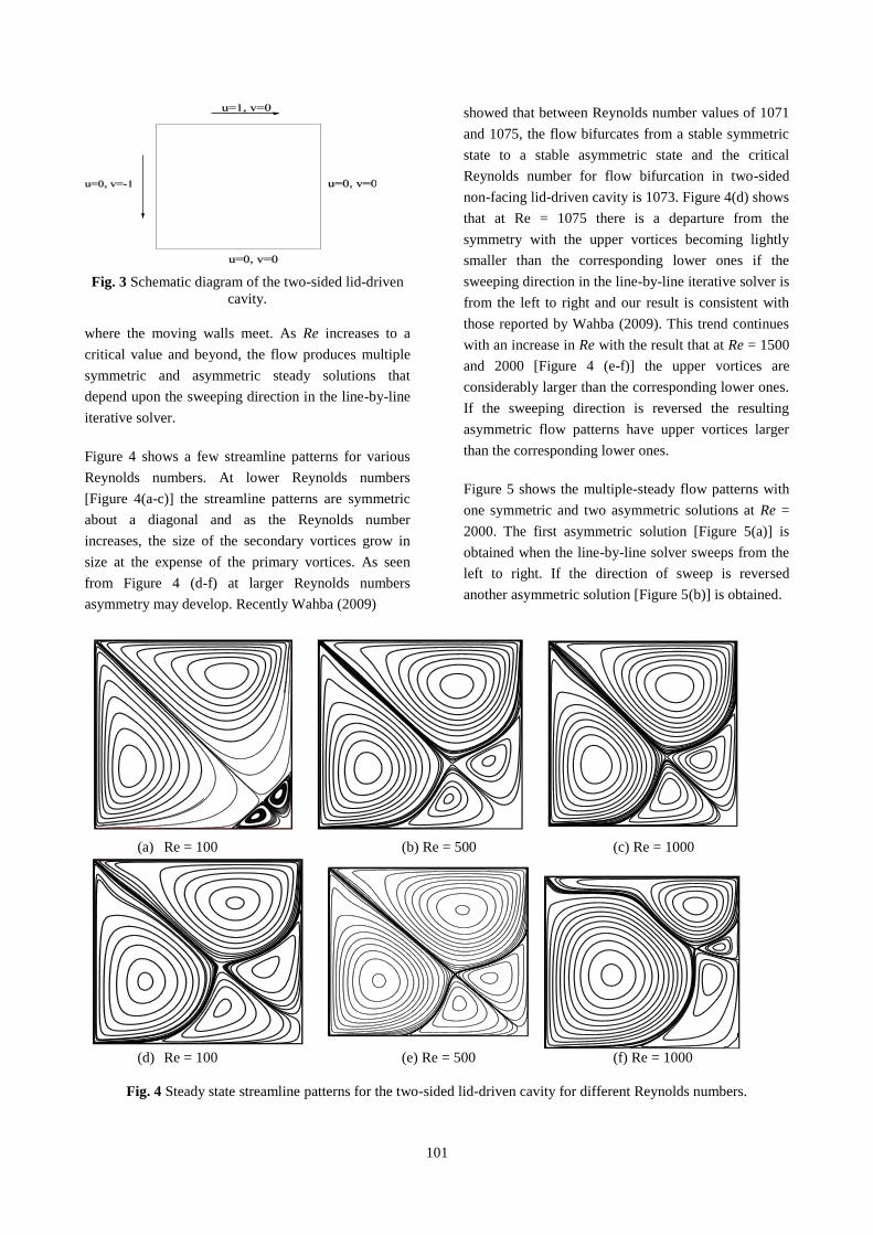
Fig. 3 Schematic diagram of the two-sided lid-driven
cavity.
where the moving walls meet. As Re increases to a
critical value and beyond, the flow produces multiple
symmetric and asymmetric steady solutions that
depend upon the sweeping direction in the line-by-line
iterative solver.
Figure 4 shows a few streamline patterns for various
Reynolds numbers. At lower Reynolds numbers
[Figure 4(a-c)] the streamline patterns are symmetric
about a diagonal and as the Reynolds number
increases, the size of the secondary vortices grow in
size at the expense of the primary vortices. As seen
from Figure 4 (d-f) at larger Reynolds numbers
asymmetry may develop. Recently Wahba (2009)
showed that between Reynolds number values of 1071
and 1075, the flow bifurcates from a stable symmetric
state to a stable asymmetric state and the critical
Reynolds number for flow bifurcation in two-sided
non-facing lid-driven cavity is 1073. Figure 4(d) shows
that at Re = 1075 there is a departure from the
symmetry with the upper vortices becoming lightly
smaller than the corresponding lower ones if the
sweeping direction in the line-by-line iterative solver is
from the left to right and our result is consistent with
those reported by Wahba (2009). This trend continues
with an increase in Re with the result that at Re = 1500
and 2000 [Figure 4 (e-f)] the upper vortices are
considerably larger than the corresponding lower ones.
If the sweeping direction is reversed the resulting
asymmetric flow patterns have upper vortices larger
than the corresponding lower ones.
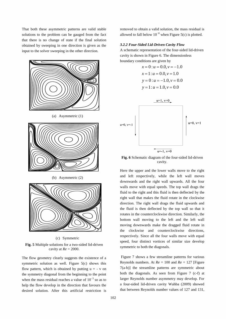
Figure 5 shows the multiple-steady flow patterns with
one symmetric and two asymmetric solutions at Re =
2000. The first asymmetric solution [Figure 5(a)] is
obtained when the line-by-line solver sweeps from the
left to right. If the direction of sweep is reversed
another asymmetric solution [Figure 5(b)] is obtained.
(a) Re = 100 (b) Re = 500 (c) Re = 1000
(d) Re = 100 (e) Re = 500 (f) Re = 1000
Fig. 4 Steady state streamline patterns for the two-sided lid-driven cavity for different Reynolds numbers.
102
That both these asymmetric patterns are valid stable
solutions to the problem can be gauged from the fact
that there is no change of state if the final solution
obtained by sweeping in one direction is given as the
input to the solver sweeping in the other direction.
(a) Asymmetric (1)
(b) Asymmetric (2)
(c) Symmetric
Fig. 5 Multiple solutions for a two-sided lid-driven
cavity at Re = 2000.
The flow geometry clearly suggests the existence of a
symmetric solution as well. Figure 5(c) shows this
flow pattern, which is obtained by putting u = - v on
the symmetry diagonal from the beginning to the point
when the mass residual reaches a value of 10−3
so as to
help the flow develop in the direction that favours the
desired solution. After this artificial restriction is
removed to obtain a valid solution, the mass residual is
allowed to fall below 10−8
when Figure 5(c) is plotted.
3.2.2 Four-Sided Lid-Driven Cavity Flow
A schematic representation of the four-sided lid-driven
cavity is shown in Figure 6. The dimensionless
boundary conditions are given by
0 : 0.0, 1.0
1: 0.0, 1.0
0 : 1.0, 0.0
1: 1.0, 0.0
x u v
x u v
y u v
y u v
Fig. 6 Schematic diagram of the four-sided lid-driven
cavity.
Here the upper and the lower walls move to the right
and left respectively, while the left wall moves
downwards and the right wall upwards. All the four
walls move with equal speeds. The top wall drags the
fluid to the right and this fluid is then deflected by the
right wall that makes the fluid rotate in the clockwise
direction. The right wall drags the fluid upwards and
the fluid is then deflected by the top wall so that it
rotates in the counterclockwise direction. Similarly, the
bottom wall moving to the left and the left wall
moving downwards make the dragged fluid rotate in
the clockwise and counterclockwise directions,
respectively. Since all the four walls move with equal
speed, four distinct vortices of similar size develop
symmetric to both the diagonals.
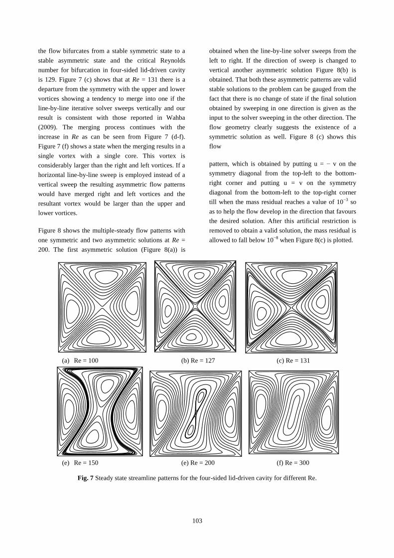
Figure 7 shows a few streamline patterns for various
Reynolds numbers. At Re = 100 and Re = 127 [Figure
7(a-b)] the streamline patterns are symmetric about
both the diagonals. As seen from Figure 7 (c-f) at
larger Reynolds number asymmetry may develop. For
a four-sided lid-driven cavity Wahba (2009) showed
that between Reynolds number values of 127 and 131,
103
the flow bifurcates from a stable symmetric state to a
stable asymmetric state and the critical Reynolds
number for bifurcation in four-sided lid-driven cavity
is 129. Figure 7 (c) shows that at Re = 131 there is a
departure from the symmetry with the upper and lower
vortices showing a tendency to merge into one if the
line-by-line iterative solver sweeps vertically and our
result is consistent with those reported in Wahba
(2009). The merging process continues with the
increase in Re as can be seen from Figure 7 (d-f).
Figure 7 (f) shows a state when the merging results in a
single vortex with a single core. This vortex is
considerably larger than the right and left vortices. If a
horizontal line-by-line sweep is employed instead of a
vertical sweep the resulting asymmetric flow patterns
would have merged right and left vortices and the
resultant vortex would be larger than the upper and
lower vortices.
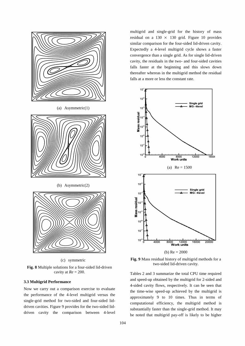
Figure 8 shows the multiple-steady flow patterns with
one symmetric and two asymmetric solutions at Re =
200. The first asymmetric solution (Figure 8(a)) is
obtained when the line-by-line solver sweeps from the
left to right. If the direction of sweep is changed to
vertical another asymmetric solution Figure 8(b) is
obtained. That both these asymmetric patterns are valid
stable solutions to the problem can be gauged from the
fact that there is no change of state if the final solution
obtained by sweeping in one direction is given as the
input to the solver sweeping in the other direction. The
flow geometry clearly suggests the existence of a
symmetric solution as well. Figure 8 (c) shows this
flow
pattern, which is obtained by putting u = − v on the
symmetry diagonal from the top-left to the bottom-
right corner and putting u = v on the symmetry
diagonal from the bottom-left to the top-right corner
till when the mass residual reaches a value of 10−3
so
as to help the flow develop in the direction that favours
the desired solution. After this artificial restriction is
removed to obtain a valid solution, the mass residual is
allowed to fall below 10−8
when Figure 8(c) is plotted.
(a) Re = 100 (b) Re = 127 (c) Re = 131
(e) Re = 150 (e) Re = 200 (f) Re = 300
Fig. 7 Steady state streamline patterns for the four-sided lid-driven cavity for different Re.
104
(a) Asymmetric(1)
(b) Asymmetric(2)
(c) symmetric
Fig. 8 Multiple solutions for a four-sided lid-driven
cavity at Re = 200.
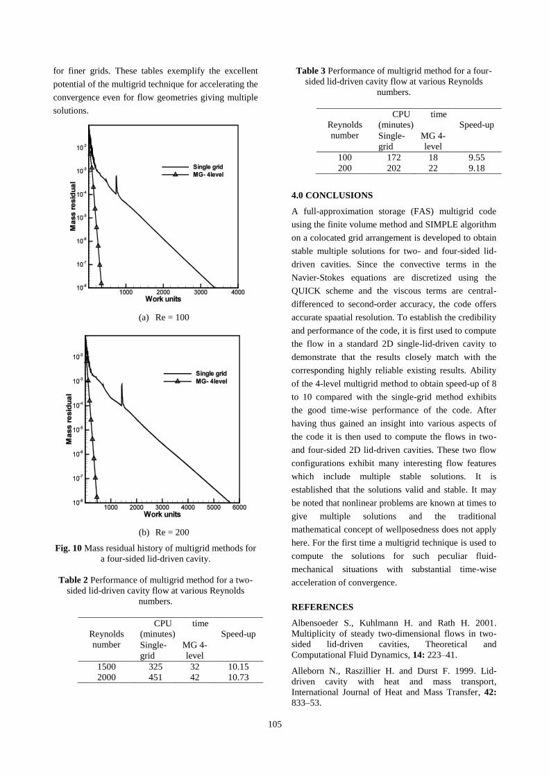
3.3 Multigrid Performance
Now we carry out a comparison exercise to evaluate
the performance of the 4-level multigrid versus the
single-grid method for two-sided and four-sided lid-
driven cavities. Figure 9 provides for the two-sided lid-
driven cavity the comparison between 4-level
multigrid and single-grid for the history of mass
residual on a 130 130 grid. Figure 10 provides
similar comparison for the four-sided lid-driven cavity.
Expectedly a 4-level multigrid cycle shows a faster
convergence than a single grid. As for single lid-driven
cavity, the residuals in the two- and four-sided cavities
falls faster at the beginning and this slows down
thereafter whereas in the multigrid method the residual
falls at a more or less the constant rate.
(a) Re = 1500
(b) Re = 2000
Fig. 9 Mass residual history of multigrid methods for a
two-sided lid-driven cavity.
Tables 2 and 3 summarize the total CPU time required
and speed-up obtained by the multigrid for 2-sided and
4-sided cavity flows, respectively. It can be seen that
the time-wise speed-up achieved by the multigrid is
approximately 9 to 10 times. Thus in terms of
computational efficiency, the multigrid method is
substantially faster than the single-grid method. It may
be noted that multigrid pay-off is likely to be higher
105
for finer grids. These tables exemplify the excellent
potential of the multigrid technique for accelerating the
convergence even for flow geometries giving multiple
solutions.
(a) Re = 100
(b) Re = 200
Fig. 10 Mass residual history of multigrid methods for
a four-sided lid-driven cavity.
Table 2 Performance of multigrid method for a two-
sided lid-driven cavity flow at various Reynolds
numbers.
Reynolds
number
CPU time
(minutes)
Speed-up Single-
grid MG 4-
level 1500
2000 325
451 32
42 10.15
10.73
Table 3 Performance of multigrid method for a four-
sided lid-driven cavity flow at various Reynolds
numbers.
Reynolds
number
CPU time
(minutes)
Speed-up Single-
grid MG 4-
level 100
200 172
202 18
22 9.55
9.18
4.0 CONCLUSIONS
A full-approximation storage (FAS) multigrid code
using the finite volume method and SIMPLE algorithm
on a colocated grid arrangement is developed to obtain
stable multiple solutions for two- and four-sided lid-
driven cavities. Since the convective terms in the
Navier-Stokes equations are discretized using the
QUICK scheme and the viscous terms are central-
differenced to second-order accuracy, the code offers
accurate spaatial resolution. To establish the credibility
and performance of the code, it is first used to compute
the flow in a standard 2D single-lid-driven cavity to
demonstrate that the results closely match with the
corresponding highly reliable existing results. Ability
of the 4-level multigrid method to obtain speed-up of 8
to 10 compared with the single-grid method exhibits
the good time-wise performance of the code. After
having thus gained an insight into various aspects of
the code it is then used to compute the flows in two-
and four-sided 2D lid-driven cavities. These two flow
configurations exhibit many interesting flow features
which include multiple stable solutions. It is
established that the solutions valid and stable. It may
be noted that nonlinear problems are known at times to
give multiple solutions and the traditional
mathematical concept of wellposedness does not apply
here. For the first time a multigrid technique is used to
compute the solutions for such peculiar fluid-
mechanical situations with substantial time-wise
acceleration of convergence.
REFERENCES
Albensoeder S., Kuhlmann H. and Rath H. 2001.
Multiplicity of steady two-dimensional flows in two-
sided lid-driven cavities, Theoretical and
Computational Fluid Dynamics, 14: 223–41.
Alleborn N., Raszillier H. and Durst F. 1999. Lid-
driven cavity with heat and mass transport,
International Journal of Heat and Mass Transfer, 42:
833–53.
106
Auteri F., Parolini N. and Quartapelle L. 2002.
Numerical investigation on the stability of singular
driven cavity flow. Journal of Computational Physics,
183: 1–25.
Barragy E. and Carey G. 1997. Streamfunction
vorticity driven cavity solution using p finite elements.
Computers and Fluids, 26: 453–68.
Botella B. and Peyret R. 1998. Benchmark spectral
results on the lid-driven cavity flow. Computers and
Fluids 27: 421–33.
Brandt A. 1977. Multilevel adaptive solutions to
boundary-value problems, Mathematics of
Computation, 31: 333–90.
Bruneau C. and Jouron C. 1990. An efficient scheme
for solving steady incompressible NavierStokes
equations. Journal of Computational Physics, 89: 389–
13.
Bruneau C. and Saad M. 2006. The 2D lid-driven
cavity problem revisited. Computers and Fluids, 35:
326–48.
Cadou J.M., Guevel Y. and Girault G. 2012.
Numerical tools for the stability analysis of 2D flows:
application to the two- and four-sided lid-driven
cavity, Fluid Dynamics Research, 44:
doi:10.1088/0169-5983/44/3/031403
Erturk E., Corke T. and Gokcol C. 2005. Numerical
solutions of 2-D steady incompressible driven cavity
flow at high Reynolds numbers.International Journal
for Numerical Methods in Fluids, 48: 747–74.
Fedorenko R. 1962. A relaxation method for solving
elliptic difference equations, Computational
Mathematics and Mathematical Physics, 1: 1092–96.
Fedorenko R. 1964. The speed of convergence of one
iteration process Computational Mathematics and
Mathematical Physics, 4, 227–35.
Ghia U., Ghia K. and Shin C. 1982. High-Resolutions
for incompressible Navier-Stokes equation and a
multigrid method. Journal of Computational Physics,
48: 387–411.
Hackbusch W. 1978. On the multigrid method applied
to difference equation, Computing, 20: 291–306.
Hayase T., Humphrey J.A.C. and Grief R. 1992. A
consistently formulated QUICK scheme for fast and
stable convergence using finite-volume iterative
calculation procedures. Journal of Computational
Physics, 98: 108–18.
Hortmann M. and Peric M. 1990, Finite volume
multigrid prediction of laminar natural
convection:Bench-mark solutions. International
Journal for Numerical Methods in Fluids, 11: 189–207.
Kalita J., Dalal D. and Dass A. 2002. A class of higher
order compact schemes for the unsteady two-
dimensional convection diffusion equation with
variable convection coefficients.International Journal
for Numerical Methods in Fluids, 38: 1111–31.
Kuhlmann H., Wanschura M. and Rath H. 1997. Flow
in two-sided lid-driven cavities: Nonuniqueness,
instabilities, and cellular structures, Journal of Fluid
Mechanics, 336: 267–99.
Kuhlmann H., Wanschura M. and Rath H.
1998. Elliptic instability in two-sided lid-driven cavity
flow, European Journal of Mechanics - B/Fluids, 17:
561–69.
Leonard B. 1979. A stable and accurate convective
modeling procedure based on quadratic upstream
interpolation, Computing Methods in Applied
Mechanics and Engineering, 19: 59–98.
Lien F. and Leschziner M. 1994. Multigrid
acceleration for recirculating laminar and turbulent
flows computed with a non-orthogonal collocated
finite volume scheme.Computational Methods in
Applied Mechanics and Engfineering, 118: 351-71.
Luo W. and Yang R. 2007. Multiple fluid flow and
heat transfer solutions in a two-sided liddriven cavity,
International Journal of Heat and Mass Transfer, 50:
2394–405.
Namprai A. and Witayangkurn S. 2012. Fluid Flow
and heat transfer in square cavities with discrete two
source-sink pairs, Advanced Studies in Theoritical
Physiscs, 6: 743-53.
Patankar S. and Spalding D. 1972. A calculation
procedure for heat, mass and momentum transfer in
three-dimensional parabolic flows, International
Journal of Heat and Mass Transfer, 15: 1787–806.
Rhie C. and Chow W. 1983. A numerical study of the
turbulent flow past an iosolated airfoil with trailing
edge separation. AIAA Journal, 21: 1525–32.
Santhosh K.D., Dass A.K. and Dewan A. 2009.
Analysis of Non-Darcy Models for Mixed Convection
in a Porous Cavity Using a Multigrid Approach,
Numerical Heat Transfer, Part A, 56: 685-708.
Sivaloganathan S. and Shaw G. 1988. A multigrid
method for recirculating flows, International Journal
for Numerical Methods in Fluids, 8: 417–40.
Wahba E. 2009. Multiplicity of states for two-sided
and four-sided lid driven cavity flows. Computers and
Fluids, 38: 247–53.
Yan J. and Thiele F. 1998. Performance and accuracy
of a modified full multigrid algorithm for fluid flow
and heat transfer.Numerical Heat Transfer: Part B, 34:
323–38.