multiple regression exercises - lycoming...

Multiple Regression Exercises 1

Multiple Regression Exercises 1. In a study to predict the sale price of a residential property (dollars),

data is taken on 20 randomly selected properties. The potential predictors in the study are appraised land value (dollars), appraised value of improvements (dollars), and area of property living space (square feet), and the data is stored in the SPSS data file realestate (which can be accessed from the appropriate link on the course syllabus web page). A 0.05 significance level is chosen for hypothesis testing.

(a) Does the data appear to be observational or experimental? Since the land value, improvement value, and area are all random, the data is observational. (b) Use SPSS to do the calculations needed for a multiple linear regression by going to the document titled Using SPSS for Windows (which can be accessed from the appropriate link on the course syllabus web page), going to the section titled Hypothesis Tests Involving Two or More Variables, and reading the steps in the subsection titled Performing a Multiple Linear Regression with Checks for Multicollinearity and of Linearity, Homoscedasticity, and Normality Assumptions; note that since there are no dummy variables in this multiple regression model, Step 7 can be skipped. Once you have successfully generated SPSS output, add a title to the top of the output in the following format: YOUR NAME – Multiple Regression Exercise 1(b) Verify that your SPSS output contains all of the following:


1. - continued


1. - continued (c) Use the SPSS output to make a statement concerning whether each of the following assumptions in a multiple linear regression is satisfied: the linearity assumption For each of the predictors land value, improvements, and area, the data points appear to be randomly distributed about the least squares line on the corresponding scatter plot. Consequently, the linearity assumption appears to be satisfied. the uniform variance (homoscedasticity) assumption The variation in standardized residuals plotted against standardized predicted values looks reasonably uniform around the horizontal line. the normality assumption The histogram of standardized residuals looks somewhat bell-shaped, and the points on the normal probability plot do not seem to depart too far from the diagonal line. Since the necessary assumptions appear to be satisfied, we feel it is appropriate to proceed with the multiple regression analysis.


1. - continued (d) Use the SPSS output to make a statement concerning whether significant multicollinearity is likely to be present in the multiple regression. Since the correlation matrix does not contain any correlation greater than 0.8 for any pair of independent variables, and tolerance > 0.10 (i.e., VIF < 10) for each independent variable, there is no indication that multicollinearity will be a problem. (e) Write the results of the f test in the ANOVA table for the regression to predict the sale price with all three potential predictors in the model; write these results in a format suitable for a journal article to be submitted for publication. The f test in the ANOVA for the regression to predict sale price from land value, improvements, and area is statistically significant at the 0.05 level (f3, 16 = 46.662, f3, 16; 0.05 = 3.24, p < 0.001). We conclude that the overall regression is significant (i.e., at least one coefficient in the regression is different from zero). (f) It is decided to use stepwise regression to select the most important predictors to include in the model. Use SPSS to do the calculations needed for a stepwise regression by going to the document titled Using SPSS for Windows (which can be accessed from the appropriate link on the course syllabus web page), going to the section titled Hypothesis Tests Involving Two or More Variables, and reading the steps in the subsection titled Performing a Stepwise Regression (or Related Procedure) to Build a Model; note that since there are no dummy variables in this multiple regression model, Step 2 can be skipped. Once you have successfully generated SPSS output, add a title to the top of the output in the following format: YOUR NAME – Multiple Regression Exercise 1(f) Verify that your SPSS output contains all of the following:


1. - continued


1. - continued

(g) Write the results of the stepwise regression in a format suitable for a journal article to be submitted for publication; include information about the significance level used and changes in R2. There were two steps in the stepwise multiple regression with a 0.05 significance level for entry and a 0.10 significance level for removal. In the first step, the variable “appraised value of improvements” was entered, which explained 83.8% of the variance in “sale price”. In the second step, the variable “area of property living space” was entered, which explained an additional 4.3% of the variance in “sale price”. No variable was removed. The two independent variables in this final step explained a total of 88.1% of the variance in “sale price”.


1. - continued (h) Write the estimated regression equation from the final step of the stepwise regression, and use this regression equation to predict the sale price of a residential property where the appraised land value is $8000, the appraised value of improvements is $20,000, and area of property living space is 1200 square feet. ̂ sale_prc = 97.521 + 0.960(impr_val) + 16.373(area) 97.521 + 0.960(20000) + 16.373(1200) = $38,945.12 (i) For each of the estimated regression coefficients in the estimated regression equation from the final step of the stepwise multiple regression, write a one sentence interpretation describing what the coefficient estimates. For each increase of one dollar in appraised value of improvements, the sale price increases on average by about $0.96. For each increase of one square foot in area of property living space, the sale price increases on average by about $16.37.


1. - continued (j) From the Correlations table of the SPSS output, find the ordinary correlation between the dependent variable sale price and the first independent variable entered into the model. The correlation between sale price and appraised value of improvements is 0.916 (k) From the Excluded Variables table of the SPSS output, find the partial correlation between the dependent variable sale price and the second independent variable entered into the model given the first independent variable entered into the model; compare this to the ordinary correlation between the dependent variable sale price and the second independent variable entered into the model, which can be found from the Correlations table of the SPSS output. The partial correlation between sale price and area of property living space given appraised value of improvements is 0.515. The ordinary correlation between sale price and area of property living space is 0.849.


2. In a study to predict the drying time (hours) for an outdoor house paint, data is taken on 22 house painting jobs. The potential predictors in the study are temperature (degrees Fahrenheit), humidity (percent), wind velocity (miles per hour), and barometric pressure, and the data is stored in the SPSS data file paint (which can be accessed from the appropriate link on the course syllabus web page). A 0.05 significance level is chosen for hypothesis testing.

(a) Does the data appear to be observational or experimental? Since the temperature, humidity, wind velocity, and barometric pressure are all random, the data is observational. (b) Use SPSS to do the calculations needed for a multiple linear regression by going to the document titled Using SPSS for Windows (which can be accessed from the appropriate link on the course syllabus web page), going to the section titled Hypothesis Tests Involving Two or More Variables, and reading the steps in the subsection titled Performing a Multiple Linear Regression with Checks for Multicollinearity and of Linearity, Homoscedasticity, and Normality Assumptions; note that since there are no dummy variables in this multiple regression model, Step 7 can be skipped. Once you have successfully generated SPSS output, add a title to the top of the output in the following format: YOUR NAME – Multiple Regression Exercise 2(b) Verify that your SPSS output contains all of the following: four scatter plots, each displaying the least squares line for one of the quantitative predictors; tables titled Descriptive Statistics, Correlations, Model Summary, ANOVA , and Coefficients; a normal probability plot; a histogram on which a bell-shaped curve has been superimposed; a plot of standardized predicted values versus standardized residuals.


2. - continued Create a Word document named Multiple_Regression_Result_Summaries with a section titled Multiple Regression Exercises 2. In this section, create a subsection for each of parts (c), (d), and (e) which follow, and in each subsection created, write the summaries for the corresponding part. Print the page(s) and insert them immediately after this page. (c) Use the SPSS output to make a statement concerning whether each of the following assumptions in a multiple linear regression is satisfied: the linearity assumption the uniform variance (homoscedasticity) assumption the normality assumption (d) Use the SPSS output to make a statement concerning whether significant multicollinearity is likely to be present in the multiple regression. (e) Write the results of the f test in the ANOVA table for the regression to predict the drying time with all four potential predictors in the model; write these results in a format suitable for a journal article to be submitted for publication.


2. - continued (f) It is decided to use stepwise regression to select the most important predictors to include in the model. Use SPSS to do the calculations needed for a stepwise regression by going to the document titled Using SPSS for Windows (which can be accessed from the appropriate link on the course syllabus web page), going to the section titled Hypothesis Tests Involving Two or More Variables, and reading the steps in the subsection titled Performing a Stepwise Regression (or Related Procedure) to Build a Model; note that since there are no dummy variables in this multiple regression model, Step 2 can be skipped. Once you have successfully generated SPSS output, add a title to the top of the output in the following format: YOUR NAME – Multiple Regression Exercise 2(f) Verify that your SPSS output contains all of the following: a table titled Variables Entered/Removed; a table titled Model Summary; a table titled ANOVA ; a table titled Coefficients; a table titled Excluded Variables. (g) In the section titled Multiple Regression Exercises 2 of the Word document named Multiple_Regression_Result_Summaries (previously created), add a subsection for this part where you write the results of the stepwise regression in a format suitable for a journal article to be submitted for publication; include information about the significance level used and changes in R2.


2. - continued (h) Write the estimated regression equation from the final step of the stepwise regression, and use this regression equation to predict drying time with a temperature of 75 degrees Fahrenheit, a relative humidity of 55%, a wind velocity of 15 miles per hour, and a barometric pressure of 759.78. ̂ drying time = 74.441 − 0.397(temperature) − 0.628(wind velocity) drying time = 74.441 − 0.397(75) − 0.628(15) = 35.246 hours (i) For each of the estimated regression coefficients in the estimated regression equation from the final step of the stepwise multiple regression, write a one sentence interpretation describing what the coefficient estimates. For each increase of one degree Fahrenheit in temperature, the drying time decreases on average by about 0.397 hours. For each increase of one mile per hour in wind velocity, the drying time decreases on average by about 0.628 hours.


2. - continued (j) From the Correlations table of the SPSS output, find the ordinary correlation between the dependent variable paint drying time and the first independent variable entered into the model. The correlation between paint drying time and temperature is − 0.588. (k) From the Excluded Variables table of the SPSS output, find the partial correlation between the dependent variable paint drying time and the second independent variable entered into the model given the first independent variable entered into the model; compare this to the ordinary correlation between the dependent variable paint drying time and the second independent variable entered into the model, which can be found from the Correlations table of the SPSS output. The partial correlation between paint drying time and wind velocity given temperature is − 0.655. The ordinary correlation between paint drying time and wind velocity is − 0.412.


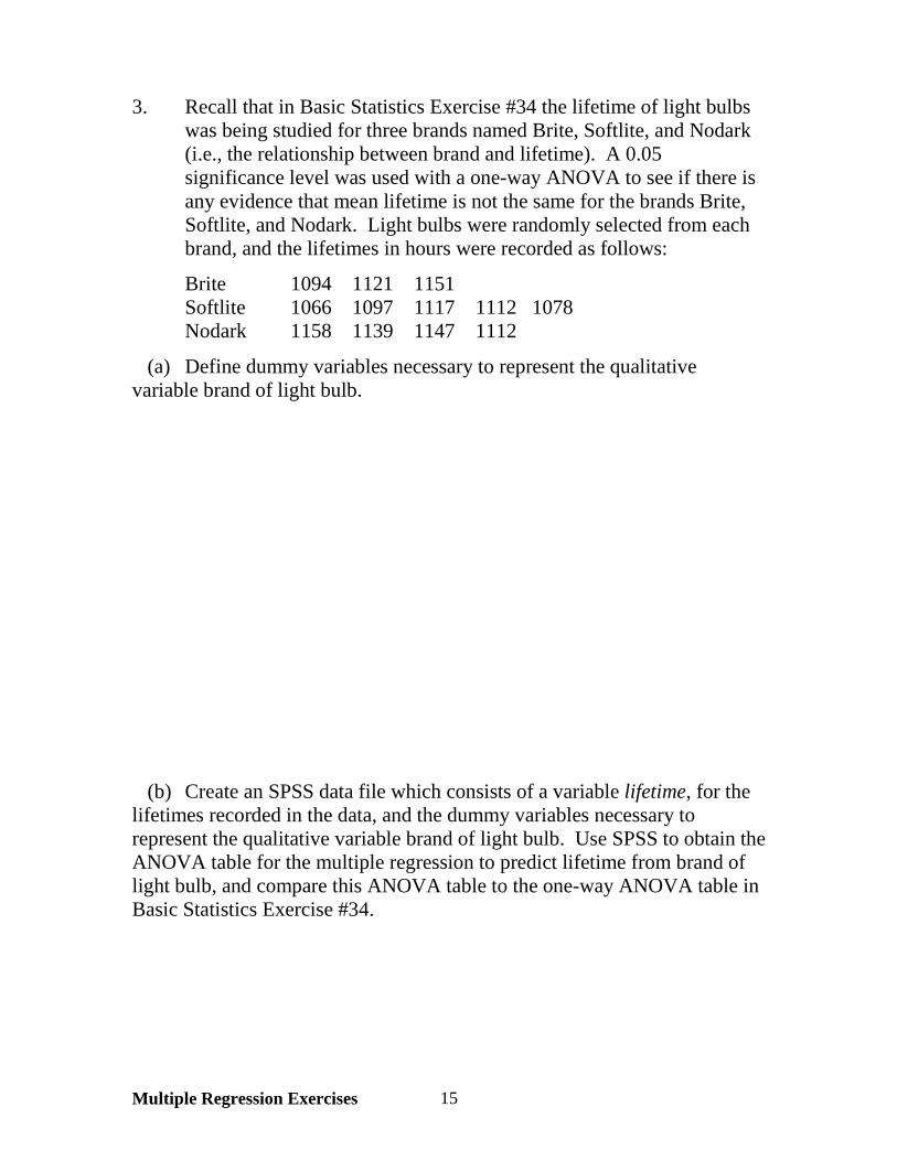
3. Recall that in Basic Statistics Exercise #34 the lifetime of light bulbs was being studied for three brands named Brite, Softlite, and Nodark (i.e., the relationship between brand and lifetime). A 0.05 significance level was used with a one-way ANOVA to see if there is any evidence that mean lifetime is not the same for the brands Brite, Softlite, and Nodark. Light bulbs were randomly selected from each brand, and the lifetimes in hours were recorded as follows:

Brite 1094 1121 1151 Softlite 1066 1097 1117 1112 1078 Nodark 1158 1139 1147 1112 (a) Define dummy variables necessary to represent the qualitative variable brand of light bulb. (b) Create an SPSS data file which consists of a variable lifetime, for the lifetimes recorded in the data, and the dummy variables necessary to represent the qualitative variable brand of light bulb. Use SPSS to obtain the ANOVA table for the multiple regression to predict lifetime from brand of light bulb, and compare this ANOVA table to the one-way ANOVA table in Basic Statistics Exercise #34.


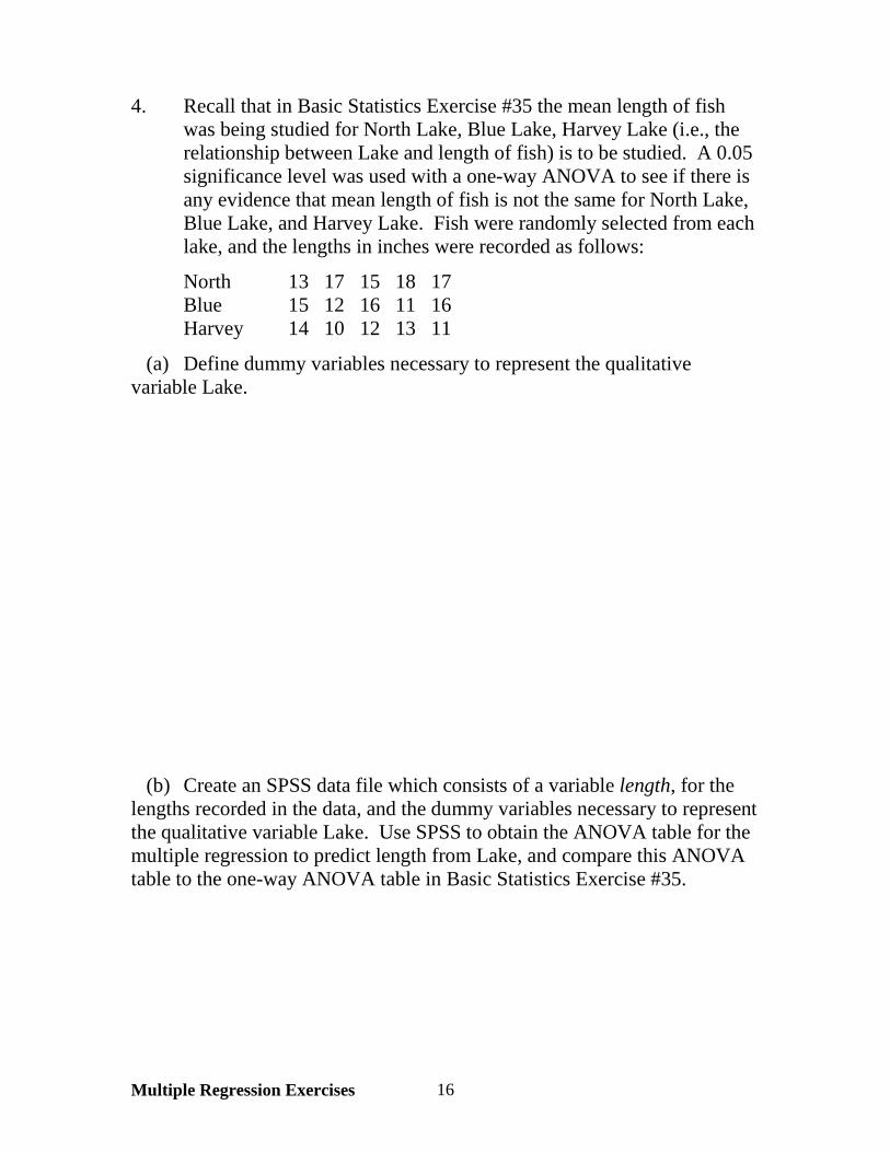
4. Recall that in Basic Statistics Exercise #35 the mean length of fish was being studied for North Lake, Blue Lake, Harvey Lake (i.e., the relationship between Lake and length of fish) is to be studied. A 0.05 significance level was used with a one-way ANOVA to see if there is any evidence that mean length of fish is not the same for North Lake, Blue Lake, and Harvey Lake. Fish were randomly selected from each lake, and the lengths in inches were recorded as follows:

North 13 17 15 18 17 Blue 15 12 16 11 16 Harvey 14 10 12 13 11 (a) Define dummy variables necessary to represent the qualitative variable Lake. (b) Create an SPSS data file which consists of a variable length, for the lengths recorded in the data, and the dummy variables necessary to represent the qualitative variable Lake. Use SPSS to obtain the ANOVA table for the multiple regression to predict length from Lake, and compare this ANOVA table to the one-way ANOVA table in Basic Statistics Exercise #35.


5. A company conducts a study to see how diastolic blood pressure is influenced by an employee’s age, weight, and job stress level classified as high stress, some stress, and low stress. Data recorded on 24 employees treated as a random sample has been stored in the SPSS data file jobstress. A 0.05 significance level is chosen for hypothesis testing.

(a) List the independent variables, and indicate whether each is quantitative or qualitative. age quantitative weight quantitative job stress level qualitative (b) Define all possible dummy variables which can be used to represent each qualitative independent variable. Any two of these indicator (dummy) variables is sufficient to represent the qualitative independent variable job stress level: 1 for high stress job X 1 = 0 for otherwise 1 for some stress job X 2 = 0 for otherwise 1 for low stress job X 3 = 0 for otherwise


5.-continued (c) In the SPSS data file jobstress, recode the variable jobtype into the first dummy defined variable in part (b), by going to the document titled Using SPSS for Windows (which can be accessed from the appropriate link on the course syllabus web page), going to the section titled Data Entry and Manipulation , and reading the steps in the subsection titled Creating New Variables by Recoding Existing Variables; then repeat this for the other dummy variable(s) in part (b), after which the data first few lines of the data file should look as follows:

(d) Use SPSS to do the calculations needed for a multiple linear regression by going to the document titled Using SPSS for Windows (which can be accessed from the appropriate link on the course syllabus web page), going to the section titled Hypothesis Tests Involving Two or More Variables, and reading the steps in the subsection titled Performing a Multiple Linear Regression with Checks for Multicollinearity and of Linearity, Homoscedasticity, and Normality Assumptions; note that Step 7 has already been completed in part (c). Once you have successfully generated SPSS output, add a title to the top of the output in the following format: YOUR NAME – Multiple Regression Exercise 5(d) Verify that your SPSS output contains all of the following:


5.-continued


5.-continued (e) Use the SPSS output to make a statement concerning whether each of the following assumptions in a multiple linear regression is satisfied: the linearity assumption For each of the quantitative predictors age and weight, the data points appear to be randomly distributed about the least squares line on the corresponding scatter plot. Consequently, the linearity assumption appears to be satisfied. the uniform variance (homoscedasticity) assumption The variation in standardized residuals plotted against standardized predicted values looks reasonably uniform around the horizontal line. the normality assumption The histogram of standardized residuals looks somewhat bell-shaped, and the points on the normal probability plot do not seem to depart too far from the diagonal line. Since the necessary assumptions appear to be satisfied, we feel it is appropriate to proceed with the multiple regression analysis.


5. - continued (f) Use the SPSS output to make a statement concerning whether significant multicollinearity is likely to be present in the multiple regression. Since the correlation matrix does not contain any correlation greater than 0.8 for any pair of independent variables, and tolerance > 0.10 (i.e., VIF < 10) for each independent variable, there is no indication that multicollinearity will be a problem. (g) Write the results of the f test in the ANOVA table for the regression to predict the diastolic blood pressure with all potential predictors in the model; write these results in a format suitable for a journal article to be submitted for publication. The f test in the ANOVA for the regression to predict diastolic blood pressure from age, weight, and indicator variables representing job stress level is statistically significant at the 0.05 level (f4, 19 = 37.953, f4, 19; 0.05 = 2.90, p < 0.001). We conclude that the overall regression is significant (i.e., at least one coefficient in the regression is different from zero). (h) It is decided to use stepwise regression to select the most important predictors to include in the model. Use SPSS to do the calculations needed for a stepwise regression by going to the document titled Using SPSS for Windows (which can be accessed from the appropriate link on the course syllabus web page), going to the section titled Hypothesis Tests Involving Two or More Variables, and reading the steps in the subsection titled Performing a Stepwise Regression (or Related Procedure) to Build a Model; note that Step 2 has already been completed in part (c). Once you have successfully generated SPSS output, add a title to the top of the output in the following format: YOUR NAME – Multiple Regression Exercise 5(f) Verify that your SPSS output contains all of the following:


5. - continued


5. - continued (i) Write the results of the stepwise regression in a format suitable for a journal article to be submitted for publication; include information about the significance level used and changes in R2. There were three steps in the stepwise multiple regression with a 0.05 significance level for entry and a 0.10 significance level for removal. In the first step, the variable weight was entered, which explained 52.8% of the variance in diastolic blood pressure. In the second step, the variable age was entered, which explained an additional 18.9% of the variance in diastolic blood pressure. No variable was removed. In the third step, the indicator variable for a high stress job was entered, which explained an additional 15.5% of the variance in diastolic blood pressure. No variable was removed. The three independent variables in this final step explained a total of 87.3% of the variance in diastolic blood pressure. (j) Write the estimated regression equation from the final step of the stepwise regression. ̂ dbp = 35.279 + 0.238(weight) + 0.559(age) + 11.871(X1) where 1 for high stress job X 1 = 0 for otherwise


5. - continued (k) For each of the estimated regression coefficients in the estimated regression equation from the final step of the stepwise multiple regression, write a one sentence interpretation describing what the coefficient estimates. For each increase of one pound in weight, diastolic blood pressure increases on average by about 0.238. For each increase of one year in age, diastolic blood pressure increases on average by about 0.559. On average, diastolic blood pressure is about 11.871 greater for employees with a high stress job than for employees with other jobs. The only indicator variable included in the model is the one for a high stress job, which suggests a statistically significant difference between the high stress job group and the other two groups combined but no statistically significant difference between the some stress job group and the low stress job group. For the high stress job group, X1 = 1 so that the least squares regression equation is ̂ dbp = 35.279 + 0.238(weight) + 0.559(age) + 11.871(1) = 47.150 + 0.238(weight) + 0.559(age) For the low stress or some stress job group, X1 = 0 so that the least squares regression equation is ̂ dbp = 35.279 + 0.238(weight) + 0.559(age) + 11.871(0) = 35.279 + 0.238(weight) + 0.559(age)


5. - continued (l) Use the estimated regression equation from the final step of the stepwise regression to predict diastolic blood pressure for each of the two following employees:

a 35-year old employee weighing 180 pounds and having a high stress job

dbp = 35.279 + 0.238(180) + 0.559(35) + 11.871(1) = 109.555

a 35-year old employee weighing 180 pounds and having a low stress or some stress job

dbp = 35.279 + 0.238(180) + 0.559(35) + 11.871(0) = 97.684 (m) From the Correlations table of the SPSS output, find the ordinary correlation between the dependent variable diastolic blood and the first independent variable entered into the model. The correlation between diastolic blood pressure and weight is 0.727. (n) From the Excluded Variables table of the SPSS output, find the partial correlation between the dependent variable diastolic blood and the second independent variable entered into the model given the first independent variable entered into the model; compare this to the ordinary correlation between the dependent variable diastolic blood and the second independent variable entered into the model, which can be found from the Correlations table of the SPSS output. The partial correlation between diastolic blood pressure and age given weight is 0.633. The ordinary correlation between diastolic blood pressure and age is 0.561.


6. In a study concerning the prediction of the wheat yield (bushels per acre), potential predictors are total rainfall (inches), average temperature (degrees Fahrenheit), and type of soil; there are three types of soil labeled A, B, and C. Data recorded on 24 employees treated as a random sample is displayed on the right. The data are from randomly selected observations over several seasons, and have been stored in the SPSS data file wheat_yield. A 0.05 significance level is chosen for hypothesis testing.

(a) List the independent variables, and indicate whether each is quantitative or qualitative. total rainfall quantitative average temperature quantitative soil type qualtitative (b) Define all possible dummy variables which can be used to represent each qualitative independent variable. Any two of these indicator (dummy) variables is sufficient to represent the qualitative independent variable job stress level: 1 for soil type A 1 for soil type B 1 for soil type C X1 = X2 = X3 = 0 otherwise 0 otherwise 0 otherwise (c) In the SPSS data file wheat_yield, recode the variable soil_typ into the first dummy defined variable in part (b), by going to the document titled Using SPSS for Windows (which can be accessed from the appropriate link on the course syllabus web page), going to the section titled Data Entry and Manipulation , and reading the steps in the subsection titled Creating New Variables by Recoding Existing Variables; then repeat this for the other dummy variable(s) in part (b).


6. - continued (d) Use SPSS to do the calculations needed for a multiple linear regression by going to the document titled Using SPSS for Windows (which can be accessed from the appropriate link on the course syllabus web page), going to the section titled Hypothesis Tests Involving Two or More Variables, and reading the steps in the subsection titled Performing a Multiple Linear Regression with Checks for Multicollinearity and of Linearity, Homoscedasticity, and Normality Assumptions; note that Step 7 has already been completed in part (c). Once you have successfully generated SPSS output, add a title to the top of the output in the following format: YOUR NAME – Multiple Regression Exercise 6(d) Verify that your SPSS output contains all of the following: two scatter plots, each displaying the least squares line for one of the quantitative predictors; tables titled Descriptive Statistics, Correlations, Model Summary, ANOVA , and Coefficients; a normal probability plot; a histogram on which a bell-shaped curve has been superimposed; a plot of standardized predicted values versus standardized residuals.


6. - continued In the Word document named Multiple_Regression_Result_Summaries (previously created), add a section titled Multiple Regression Exercises 6. In this section, create a subsection for each of parts (c), (d), and (e) which follow, and in each subsection created, write the summaries for the corresponding part. Print the page(s) and insert them immediately after this page. (e) Use the SPSS output to make a statement concerning whether each of the following assumptions in a multiple linear regression is satisfied: the linearity assumption the uniform variance (homoscedasticity) assumption the normality assumption (f) Use the SPSS output to make a statement concerning whether significant multicollinearity is likely to be present in the multiple regression. (g) Write the results of the f test in the ANOVA table for the regression to predict wheat yield with all potential predictors in the model; write these results in a format suitable for a journal article to be submitted for publication.


6. - continued (h) It is decided to use stepwise regression to select the most important predictors to include in the model. Use SPSS to do the calculations needed for a stepwise regression by going to the document titled Using SPSS for Windows (which can be accessed from the appropriate link on the course syllabus web page), going to the section titled Hypothesis Tests Involving Two or More Variables, and reading the steps in the subsection titled Performing a Stepwise Regression (or Related Procedure) to Build a Model; note that Step 2 has already been completed in part (c). Once you have successfully generated SPSS output, add a title to the top of the output in the following format: YOUR NAME – Multiple Regression Exercise 6(f) Verify that your SPSS output contains all of the following: a table titled Variables Entered/Removed; a table titled Model Summary; a table titled ANOVA ; a table titled Coefficients; a table titled Excluded Variables. (i) In the section titled Multiple Regression Exercises 6 of the Word document named Multiple_Regression_Result_Summaries (previously created), add a subsection for this part where you write the results of the stepwise regression in a format suitable for a journal article to be submitted for publication; include information about the significance level used and changes in R2.


6. - continued (j) Write the estimated regression equation from the final step of the stepwise regression. ^ yield = − 16.571 + 0.691(rain) + 0.185(temp) − 17.352(X1) (k) For each of the estimated regression coefficients in the estimated regression equation from the final step of the stepwise multiple regression, write a one sentence interpretation describing what the coefficient estimates. For each increase of one inch in total rainfall, wheat yield increases on average by about 0.691 bushels per acre. For each increase of one degree Fahrenheit in temperature, wheat yield increases on average by about 0.185 bushels per acre. On average, wheat yield is about 17.352 bushels per acre smaller with soil type A than for other soil types.


6. - continued (l) Use the estimated regression equation from the final step of the stepwise regression to predict wheat yield in each of the following scenarios:

Total rainfall is 60 inches, average temperature is 65 degrees Fahrenheit, and soil type A is used.

− 33.923 + 0.691(60) + 0.185(65) = − 33.923 + 41.46 + 12.025 = 19.562 bushels per acre

Total rainfall is 60 inches, average temperature is 65 degrees Fahrenheit, and soil type B or C is used.

− 16.571 + 0.691(60) + 0.185(65) = − 16.571 + 41.46 + 12.025 = 36.914 bushels per acre

multiple regression exercises - lycoming...

Documents