Multiple Phase Screen (MPS) Calculation of Two-way Spherical

Wave Propagation in the Ionosphere

Ionospheric Effects Symposium

May 2015

Dennis L. Knepp

NorthWest Research Associates Monterey, California

Outline

• Introduction • Formulation of the solution • Examples

– Scintillation index for two-way propagation > Monostatic geometry > Bistatic geometry

– Reciprocity – Two-way propagation with multiple correlated scatterers

• Conclusions

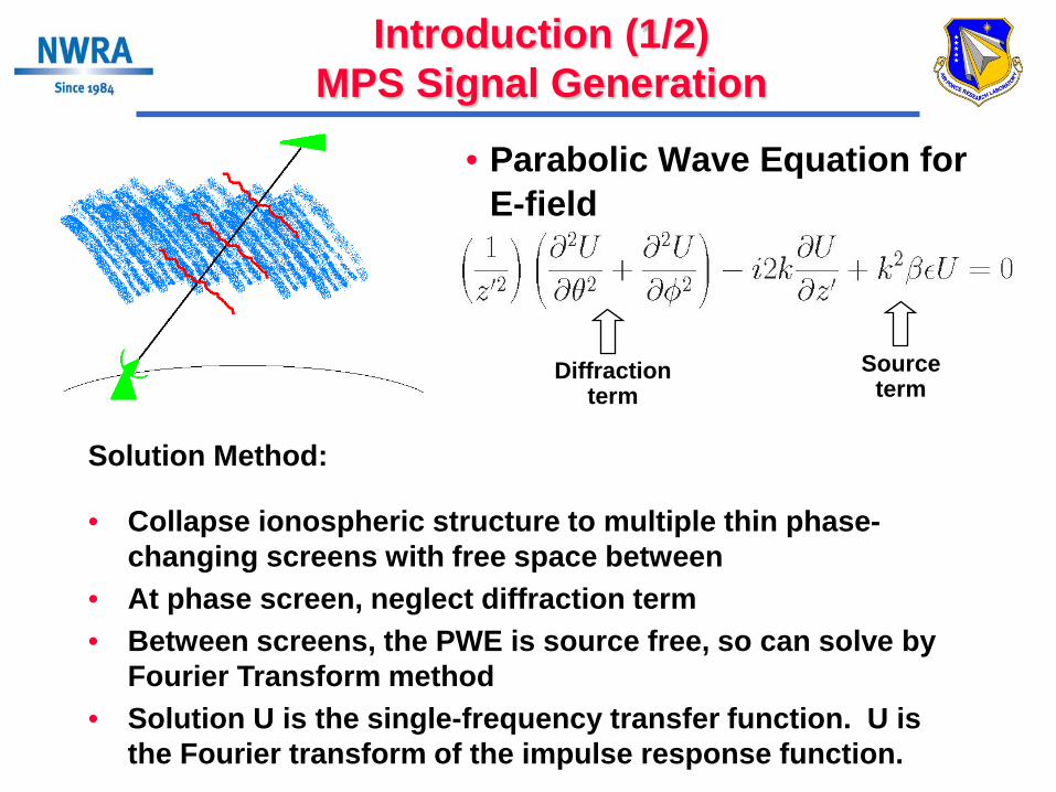
• Parabolic Wave Equation for

E-field

Solution Method:

Introduction (1/2) MPS Signal Generation

Diffraction term

Source term

• Collapse ionospheric structure to multiple thin phase-changing screens with free space between

• At phase screen, neglect diffraction term • Between screens, the PWE is source free, so can solve by

Fourier Transform method • Solution U is the single-frequency transfer function. U is

the Fourier transform of the impulse response function.

Introduction (2/2)

• Impulse response function – Convolve the impulse response function with the transmitted

waveform to obtain the received, disturbed waveform • Two methods to calculate the impulse response function:

– Statistical techniques: > Techniques based on the mutual coherence function (MCF) > Starting point is the analytic solution for the two-frequency, two-

time, two-position MCF (the correlation function of the propagating electric field)

> Theoretical calculation requires strong scattering, S4 equal to unity, phase structure function must be quadratic, signal bandwidth is small, structure is homogeneous.

> Limitations never fully studied > Previously the choice for most receiver testing because of speed

and relative simplicity. But, still in use now for strategic systems – Multiple phase screen (MPS) techniques

> Most accurate technique available. Starting point is a realization of the in-situ electron density. None of the limitations above apply.

Formulation

Scalar Helmholtz equation where

Formulation

Substitute the parabolic approximation for a spherical wave Make the substitutions To obtain the final parabolic wave equation (PWE) Propagation through a phase screen: solve PWE with diffraction term set to zero

Formulation

Free-space propagation between phase screens: set source term to zero and solve remaining equation via FFTs The solution for free-space propagation is where

Propagation Geometry Used in the Following Examples

Structured ionosphere

Five phase screens

Upward propagation

Target locations

Transmitter locations

Z = 0

Z = 600 km

Z = 200 km 20 km

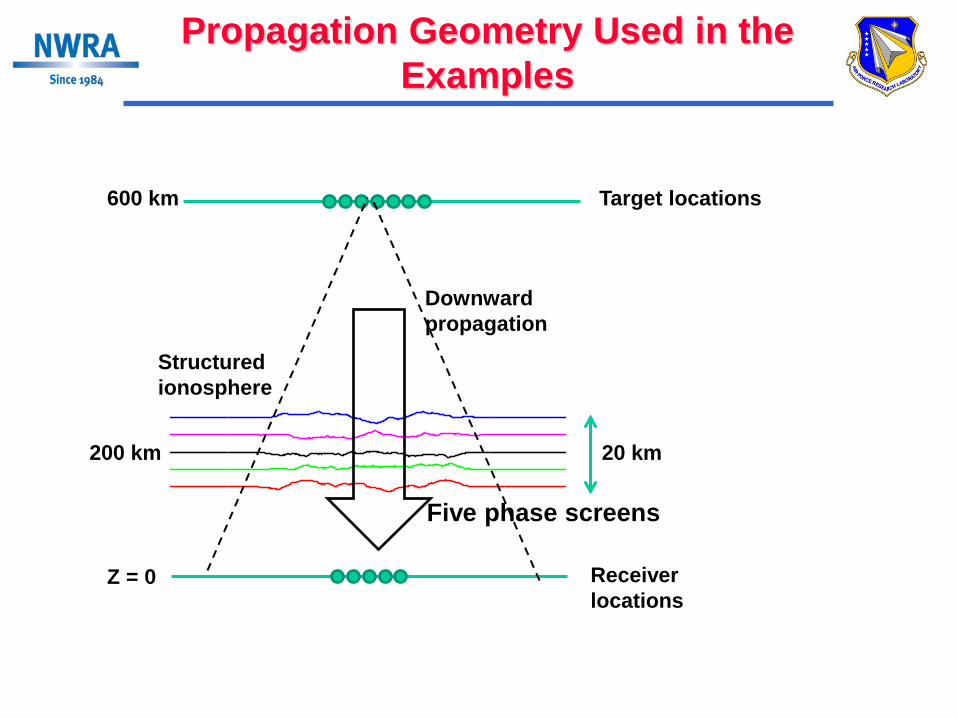
Propagation Geometry Used in the Examples

Structured ionosphere

Five phase screens

Downward propagation

Target locations

Receiver locations

Z = 0

600 km

200 km 20 km

Close-up of Five Phase Screens

• Values of phase shown are separated by 10 radians • Screens extend in altitude from 190 to 210 km • Length of phase screen at 200 km altitude is 200 km • Phase screens are generated to have a K-3 PSD, outer scale

of 5 km, inner scale of 10 m, and are comprised of 219 points.

-50 0 50

-10

0

10

20

30

40

50

60

Distance (km)

Phas

e (r

adia

ns)

g g SWP202

Distance (km)

-100 -50 0 50 100-30

-20

-10

0

10

Ampl

itude

(dB)

EandPhi Case: 202 FieldPtKm: 600SWP202

-100 -50 0 50 100-40

-20

0

20

40

60

Phas

e (r

ad)

Electric Field in the Target Plane Due to a Single Transmitter

Electric field at z = 600 km caused by a single element located at z = 0, after propagation through five phase screens

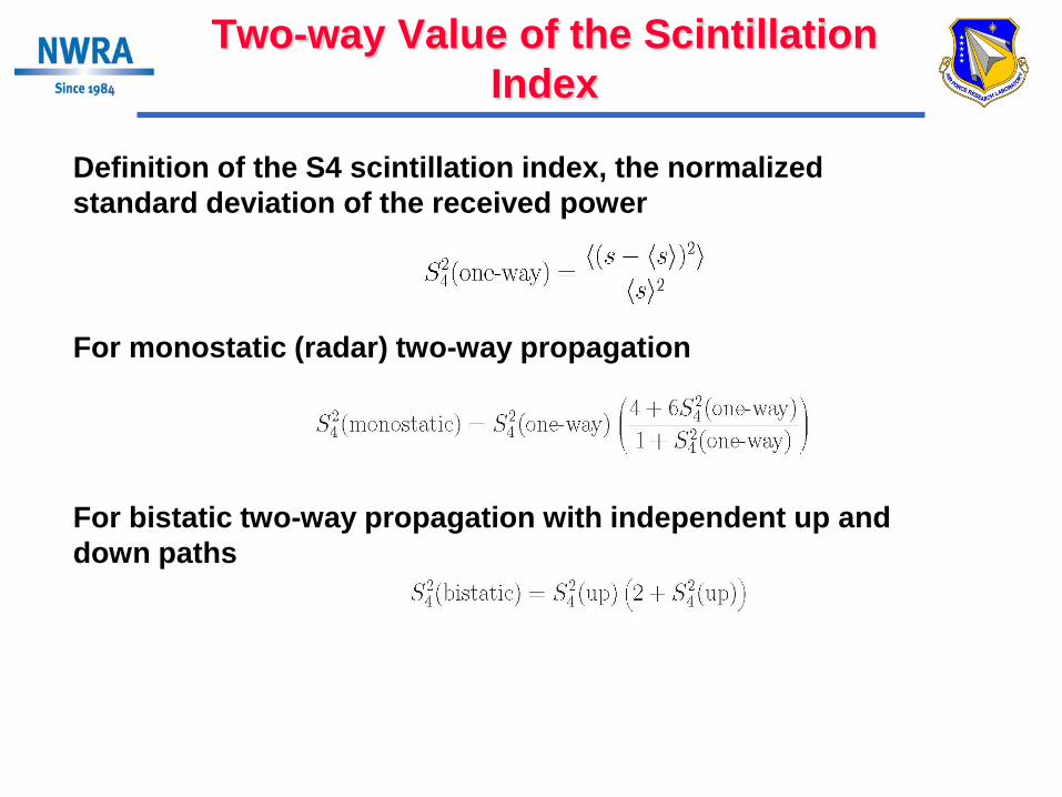
Two-way Value of the Scintillation Index

Definition of the S4 scintillation index, the normalized standard deviation of the received power For monostatic (radar) two-way propagation For bistatic two-way propagation with independent up and down paths

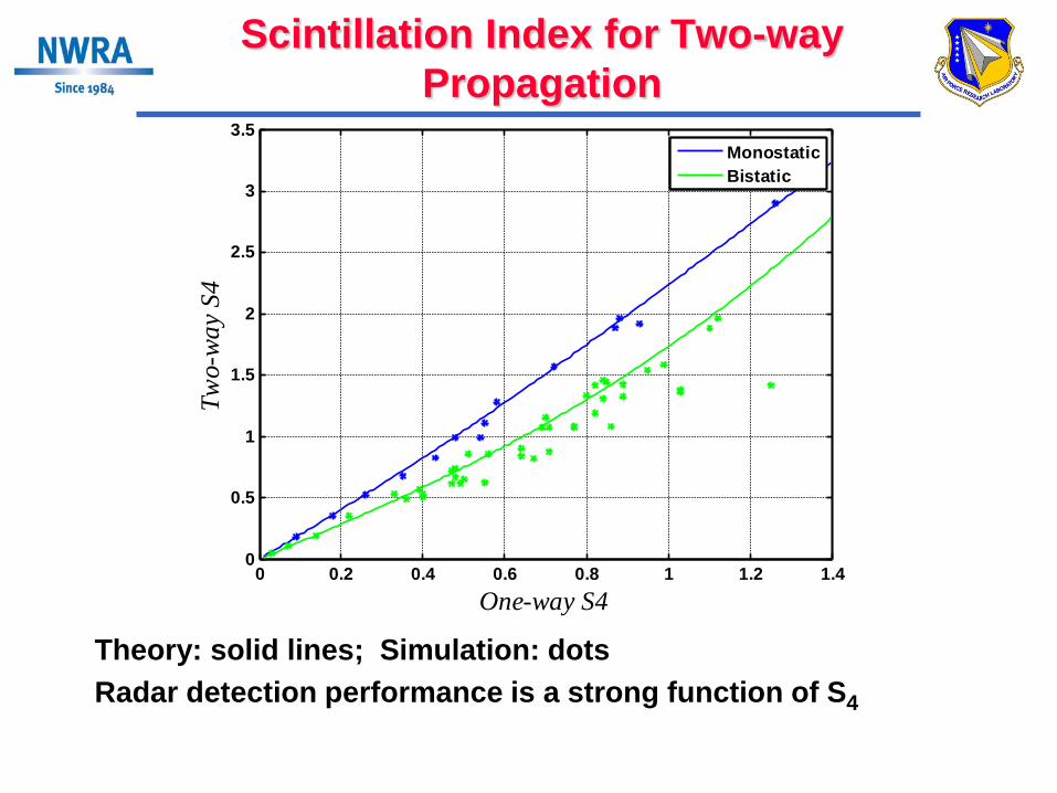
Scintillation Index for Two-way Propagation

0 0.2 0.4 0.6 0.8 1 1.2 1.40

0.5

1

1.5

2

2.5

3

3.5

One-way S4

Two-

way

S4

MonostaticBistatic

Theory: solid lines; Simulation: dots Radar detection performance is a strong function of S4

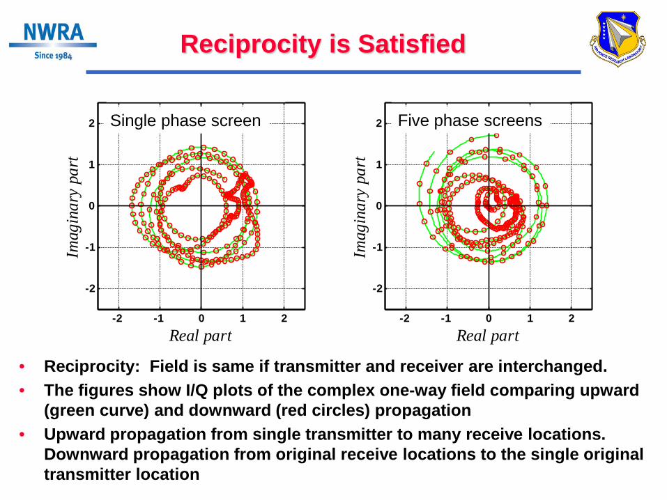
Reciprocity is Satisfied

-2 -1 0 1 2

-2

-1

0

1

2

Real part

Imag

inar

y pa

rtRecipCheck Case: 201

-2 -1 0 1 2

-2

-1

0

1

2

Real partIm

agin

ary

part

RecipCheck Case: 202

• Reciprocity: Field is same if transmitter and receiver are interchanged. • The figures show I/Q plots of the complex one-way field comparing upward

(green curve) and downward (red circles) propagation • Upward propagation from single transmitter to many receive locations.

Downward propagation from original receive locations to the single original transmitter location

Single phase screen Five phase screens

Two-way Propagation

Field at target plane due to many transmitter elements Field at receiver plane due to scatterers in target plane Following two examples of two-way propagation: One transmitter at center of MPS grid Upward propagation through five phase screens 401 target scatterers at z = 600 km, spaced by λ/2 Downward propagation back to receiver plane

Two-way Propagation, Weak Scattering, Linear Group of Scatterers

-10 -5 0 5 10-40

-20

0

20

Ampl

itude

(dB)

y

SWS205TheoryMPS code

-10 -5 0 5 100

200

400

600

Phas

e (r

ad)

-10 -5 0 5 10-5

0

5

10

Phas

e di

ff (r

ad)

-10 -5 0 5 10-100

-50

0

50

Distance (km)

AoA

(mra

d)

• 5 screens near z = 200 km

• 401 scatterers at z = 600 km

• S4(one-way) = 0.16

• Figure shows small portion of MPS grid

• Smooth red curve is theory for case of no scintillation

• Blue is MPS result • Measurement of

AoA uses 10-m antenna & correlation technique

-10 -5 0 5 10-40

-20

0

20

Ampl

itude

(dB)

y

SWS206TheoryMPS code

-10 -5 0 5 10-500

0

500

1000

Phas

e (r

ad)

-10 -5 0 5 10-5

0

5

10

Phas

e di

ff (r

ad)

-10 -5 0 5 10-20

0

20

Distance (km)

AoA

(mra

d)

Two-way Propagation, Stronger Scattering, Linear Group of Scatterers

• 5 screens near z = 200 km

• 401 scatterers at z = 600 km

• S4(one-way) = 0.46

• Figure shows small portion of MPS grid

• Smooth red curve is theory for case of no scintillation

• Blue is MPS result • Measurement of

AoA uses 10-m antenna & correlation technique

Conclusions

• Originally developed for application to synthetic aperture radar

• Includes the correlation of signals propagating on closely-spaced paths

• Avoids the small-scene approximation • Code design allows for variation in RCS of the

target scatterers • Additional but straightforward work needed for:

– 3D propagation – Application to wide bandwidth waveforms