Multiple Hypothesis Tracking Revisited

Chanho Kim † Fuxin Li ‡ † Arridhana Ciptadi † James M. Rehg †

†Georgia Institute of Technology ‡Oregon State University

Abstract

This paper revisits the classical multiple hypothesestracking (MHT) algorithm in a tracking-by-detection frame-work. The success of MHT largely depends on the abil-ity to maintain a small list of potential hypotheses, whichcan be facilitated with the accurate object detectors that arecurrently available. We demonstrate that a classical MHTimplementation from the 90’s can come surprisingly closeto the performance of state-of-the-art methods on standardbenchmark datasets. In order to further utilize the strengthof MHT in exploiting higher-order information, we intro-duce a method for training online appearance models foreach track hypothesis. We show that appearance modelscan be learned efficiently via a regularized least squaresframework, requiring only a few extra operations for eachhypothesis branch. We obtain state-of-the-art results onpopular tracking-by-detection datasets such as PETS andthe recent MOT challenge.

1. IntroductionMultiple Hypotheses Tracking (MHT) is one of the ear-

liest successful algorithms for visual tracking. Originallyproposed in 1979 by Reid [36], it builds a tree of poten-tial track hypotheses for each candidate target, thereby pro-viding a systematic solution to the data association prob-lem. The likelihood of each track is calculated and the mostlikely combination of tracks is selected. Importantly, MHTis ideally suited to exploiting higher-order information suchas long-term motion and appearance models, since the en-tire track hypothesis can be considered when computing thelikelihood.

MHT has been popular in the radar target tracking com-munity [6]. However, in visual tracking problems, it is gen-erally considered to be slow and memory intensive, requir-ing many pruning tricks to be practical. While there wasconsiderable interest in MHT in the vision community dur-ing the 90s, for the past 15 years it has not been a main-stream approach for tracking, and rarely appears as a base-

‡ This work was conducted while the 2nd author was at Georgia Tech.

line in tracking evaluations. MHT is in essence a breadth-first search algorithm, hence its performance strongly de-pends on the ability to prune branches in the search treequickly and reliably, in order to keep the number of trackhypotheses manageable. In the early work on MHT for vi-sual tracking [12], target detectors were unreliable and mo-tion models had limited utility, leading to high combinatoricgrowth of the search space and the need for efficient pruningmethods.

This paper argues that the MHT approach is well-suitedto the current visual tracking context. Modern advances intracking-by-detection and the development of effective fea-ture representations for object appearance have created newopportunities for the MHT method. First, we demonstratethat a modern formulation of a standard motion-based MHTapproach gives comparable performance to state-of-the-artmethods on popular tracking datasets. Second, and moreimportantly, we show that MHT can easily exploit high-order appearance information which has been difficult toincorporate into other tracking frameworks based on unaryand pairwise energies. We present a novel MHT methodwhich incorporates long-term appearance modeling, usingfeatures from deep convolutional neural networks [20, 16].The appearance models are trained online for each trackhypothesis on all detections from the entire history of thetrack. We utilize online regularized least squares [25] toachieve high efficiency. In our formulation, the computa-tional cost of training the appearance models has little de-pendency on the number of hypothesis branches, making itextremely suitable for the MHT approach.

Our experimental results demonstrate that our scoringfunction, which combines motion and appearance, is highlyeffective in pruning the hypothesis space efficiently and ac-curately. Using our trained appearance model, we are ableto cut the effective number of branches in each frame toabout 50% of all branches (Sec. 5.1). This enables us tomake less restrictive assumptions on motion and explore alarger space of hypotheses. This also makes MHT less sen-sitive to parameter choices and heuristics (Fig. 3). Experi-ments on the PETS and the recent MOT challenge illustratethe state-of-the-art performance of our approach.

1

2. Related WorkNetwork flow-based methods [35, 4, 45, 10] have re-

cently become a standard approach to visual multi-targettracking due to their computational efficiency and optimal-ity. In recent years, efficient inference algorithms to findthe globally optimal solution [45, 4] or approximate solu-tions [35] have been introduced. However, the benefits offlow-based approaches come with a costly restriction: thecost function can only contain unary and pairwise terms.Pairwise costs are very restrictive in representing motionand appearance. In particular, it is difficult to represent evena linear motion model with those terms.

An alternative is to define pairwise costs between track-lets – short object tracks that can be computed reliably[26, 3, 18, 8]. Unfortunately the availability of reliabletracklets cannot be guaranteed, and any mistakes propagateto the final solution. In Brendel et al. [8], data associationfor tracklets is solved using the Maximum Weighted Inde-pendent Set (MWIS) method. We also adopt MWIS, butfollow the classical formulation in [34] and focus on the in-corporation of appearance modeling.

Collins [11] showed mathematically that the multidi-mensional assignment problem is a more complete repre-sentation of the multi-target tracking problem than the net-work flow formulation. Unlike network flow, there is nolimitation in the form of the cost function, even though find-ing an exact solution to the multidimensional assignmentproblem is intractable.

Classical solutions to multidimensional assignment areMHT [36, 12, 17, 34] and Markov Chain Monte Carlo(MCMC) data association [19, 32]. While MCMC providesasymptotic guarantees, MHT has the potential to explore thesolution space more thoroughly, but has traditionally beenhindered by the exponential growth in the number of hy-potheses and had to resort to aggressive pruning strategies,such as propagating only the M -best hypotheses [12]. Wewill show that this limitation can be addressed through dis-criminative appearance modeling.

Andriyenko [1] proposed a discrete-continuous opti-mization method to jointly solve trajectory estimation anddata association. Trajectory estimation is solved by splinefitting and data association is solved via MRF inference.These two steps are alternated until convergence. Segal [37]proposed a related approach based on a message passing al-gorithm. These methods are similar to MHT in the sensethat they directly optimize a global energy with no guar-antees on solution quality. But in practice, MHT is moreeffective in identifying high quality solutions.

There have been a significant number of prior works thatexploit appearance information to solve data association. Inthe network flow-based method, the pairwise terms can beweighted by offline trained appearance templates [38] or asimple distance metric between appearance features [45].

However, these methods have limited capability to modelthe complex appearance changes of a target. In [17], a sim-ple fixed appearance model is incorporated into a standardMHT framework. In contrast, we show that MHT can be ex-tended to include online learned discriminative appearancemodels for each track hypothesis.

Online discriminative appearance modeling is a standardmethod for addressing appearance variation [39]. In trackletassociation, several works [2, 42, 21, 22] train discrimina-tive appearance models of tracklets in order to design a bet-ter affinity score function. However, these approaches stillshare the limitations of the tracklet approach. Other works[7, 40] train a classifier for each target and use the classifi-cation score for greedy data association or particle filtering.These methods only keep one online learned model for eachtarget, while our method trains multiple online appearancemodels via multiple track hypotheses, which is more robustto model drift.

3. Multiple Hypotheses Tracking

We adopt a tracking-by-detection framework such thatour observations are localized bounding boxes obtainedfrom an object detection algorithm. Let k denote the mostrecent frame and Mk denote the number of object detec-tions (i.e. observations) in that frame. For a given track,let ik denote the observation which is selected at framek, where ik ∈ {0, 1, . . . ,Mk}. The observation sequencei1, i2, . . . , ik then defines a track hypothesis over k frames.Note that the dummy assignment it = 0 represents the caseof a missing observation (due to occlusion or a false neg-ative).1 Let the binary variable zi1i2...ik denote whether ornot a track hypothesis is selected in the final solution. Aglobal hypothesis is a set of track hypotheses that are notin conflict, i.e. that do not share any measurements at anytime.

A key strategy in MHT is to delay data association de-cisions by keeping multiple hypotheses active until data as-sociation ambiguities are resolved. MHT maintains mul-tiple track trees, and each tree represents all of the hy-potheses that originate from a single observation (Fig. 1c).At each frame, the track trees are updated from observa-tions and each track in the tree is scored. The best set ofnon-conflicting tracks (the best global hypothesis) can thenbe found by solving a maximum weighted independent setproblem (Fig. 2a). Afterwards, branches that deviate toomuch from the global hypothesis are pruned from the trees,and the algorithm proceeds to the next frame. In the rest ofthis section, we will describe the approach in more detail.

1For notational convenience, observation sequences can be assumed tobe padded with zeros so that all track hypotheses can be treated as fixedlength sequences, despite their varying starting and ending times.

k

4

2

1

3

5

1

2 2

31

1

(a) Tracks in Video Frames

2

3

5

k

��怠4

1 ��態

(b) Gating

1

3 2

4 2 1 3

1

t = k

t = k-1

t = k-2

t = 1

. . .

Tree 1 Tree 2 Tree 3

2

2 1

1 3 0 5

(c) Track Trees

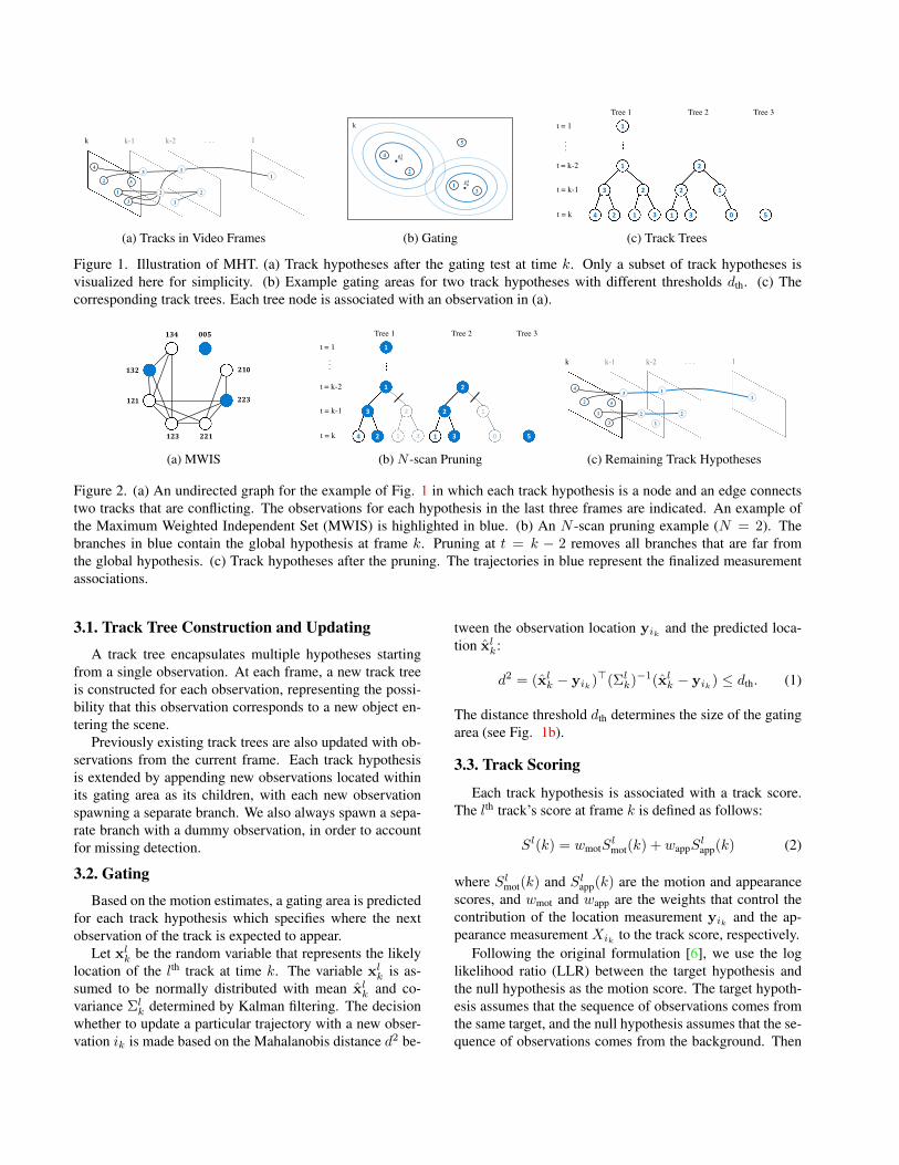
Figure 1. Illustration of MHT. (a) Track hypotheses after the gating test at time k. Only a subset of track hypotheses isvisualized here for simplicity. (b) Example gating areas for two track hypotheses with different thresholds dth. (c) Thecorresponding track trees. Each tree node is associated with an observation in (a).

層惣想層惣匝層匝1

層匝惣 匝匝層匝匝惣匝層0

宋宋捜

(a) MWIS

3

4 2

1

t = k

t = k-1

t = k-2

t = 1

. . .

Tree 1 Tree 2 Tree 3

2

2

1 3 5

1

(b) N -scan Pruning

k

4

2

1

3

5

1

2 2

31

1

(c) Remaining Track Hypotheses

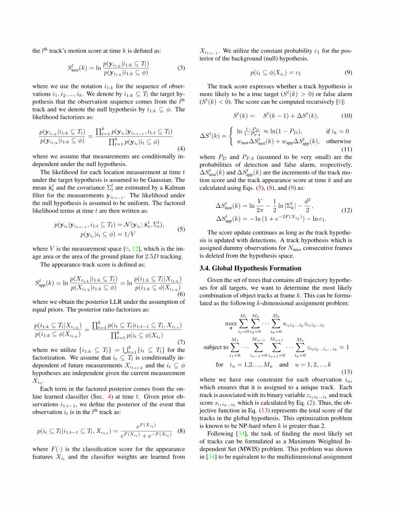
Figure 2. (a) An undirected graph for the example of Fig. 1 in which each track hypothesis is a node and an edge connectstwo tracks that are conflicting. The observations for each hypothesis in the last three frames are indicated. An example ofthe Maximum Weighted Independent Set (MWIS) is highlighted in blue. (b) An N -scan pruning example (N = 2). Thebranches in blue contain the global hypothesis at frame k. Pruning at t = k − 2 removes all branches that are far fromthe global hypothesis. (c) Track hypotheses after the pruning. The trajectories in blue represent the finalized measurementassociations.

3.1. Track Tree Construction and Updating

A track tree encapsulates multiple hypotheses startingfrom a single observation. At each frame, a new track treeis constructed for each observation, representing the possi-bility that this observation corresponds to a new object en-tering the scene.

Previously existing track trees are also updated with ob-servations from the current frame. Each track hypothesisis extended by appending new observations located withinits gating area as its children, with each new observationspawning a separate branch. We also always spawn a sepa-rate branch with a dummy observation, in order to accountfor missing detection.

3.2. Gating

Based on the motion estimates, a gating area is predictedfor each track hypothesis which specifies where the nextobservation of the track is expected to appear.

Let xlk be the random variable that represents the likely

location of the lth track at time k. The variable xlk is as-

sumed to be normally distributed with mean xlk and co-

variance Σlk determined by Kalman filtering. The decision

whether to update a particular trajectory with a new obser-vation ik is made based on the Mahalanobis distance d2 be-

tween the observation location yik and the predicted loca-tion xl

k:

d2 = (xlk − yik)>(Σl

k)−1(xlk − yik) ≤ dth. (1)

The distance threshold dth determines the size of the gatingarea (see Fig. 1b).

3.3. Track Scoring

Each track hypothesis is associated with a track score.The lth track’s score at frame k is defined as follows:

Sl(k) = wmotSlmot(k) + wappS

lapp(k) (2)

where Slmot(k) and Sl

app(k) are the motion and appearancescores, and wmot and wapp are the weights that control thecontribution of the location measurement yik and the ap-pearance measurement Xik to the track score, respectively.

Following the original formulation [6], we use the loglikelihood ratio (LLR) between the target hypothesis andthe null hypothesis as the motion score. The target hypoth-esis assumes that the sequence of observations comes fromthe same target, and the null hypothesis assumes that the se-quence of observations comes from the background. Then

the lth track’s motion score at time k is defined as:

Slmot(k) = ln

p(yi1:k |i1:k ⊆ Tl)p(yi1:k |i1:k ⊆ φ)

(3)

where we use the notation i1:k for the sequence of obser-vations i1, i2, ..., ik. We denote by i1:k ⊆ Tl the target hy-pothesis that the observation sequence comes from the lth

track and we denote the null hypothesis by i1:k ⊆ φ. Thelikelihood factorizes as:

p(yi1:k |i1:k ⊆ Tl)p(yi1:k |i1:k ⊆ φ)

=

∏kt=1 p(yit |yi1:t−1 , i1:t ⊆ Tl)∏k

t=1 p(yit |it ⊆ φ)(4)

where we assume that measurements are conditionally in-dependent under the null hypothesis.

The likelihood for each location measurement at time tunder the target hypothesis is assumed to be Gaussian. Themean xl

t and the covariance Σlt are estimated by a Kalman

filter for the measurements yi1:t−1. The likelihood under

the null hypothesis is assumed to be uniform. The factoredlikelihood terms at time t are then written as:

p(yit |yi1:t−1 , i1:t ⊆ Tl) = N (yit ; xlt,Σ

lt),

p(yit |it ⊆ φ) = 1/V(5)

where V is the measurement space [6, 12], which is the im-age area or the area of the ground plane for 2.5D tracking.

The appearance track score is defined as:

Slapp(k) = ln

p(Xi1:k |i1:k ⊆ Tl)p(Xi1:k |i1:k ⊆ φ)

= lnp(i1:k ⊆ Tl|Xi1:k)

p(i1:k ⊆ φ|Xi1:k)(6)

where we obtain the posterior LLR under the assumption ofequal priors. The posterior ratio factorizes as:

p(i1:k ⊆ Tl|Xi1:k)

p(i1:k ⊆ φ|Xi1:k)=

∏kt=1 p(it ⊆ Tl|i1:t−1 ⊆ Tl, Xi1:t)∏k

t=1 p(it ⊆ φ|Xit)(7)

where we utilize {i1:k ⊆ Tl} =⋃k

t=1{it ⊆ Tl} for thefactorization. We assume that it ⊆ Tl is conditionally in-dependent of future measurements Xit+1:k

and the it ⊆ φhypotheses are independent given the current measurementXit .

Each term in the factored posterior comes from the on-line learned classifier (Sec. 4) at time t. Given prior ob-servations i1:t−1, we define the posterior of the event thatobservation it is in the lth track as:

p(it ⊆ Tl|i1:t−1 ⊆ Tl, Xi1:t) =eF (Xit )

eF (Xit ) + e−F (Xit )(8)

where F (·) is the classification score for the appearancefeatures Xit and the classifier weights are learned from

Xi1:t−1 . We utilize the constant probability c1 for the pos-terior of the background (null) hypothesis.

p(it ⊆ φ|Xit) = c1 (9)

The track score expresses whether a track hypothesis ismore likely to be a true target (Sl(k) > 0) or false alarm(Sl(k) < 0). The score can be computed recursively [6]:

Sl(k) = Sl(k − 1) + ∆Sl(k), (10)

∆Sl(k) =

{ln 1−PD

1−PFA≈ ln(1− PD), if ik = 0

wmot∆Slmot(k) + wapp∆Sl

app(k), otherwise(11)

where PD and PFA (assumed to be very small) are theprobabilities of detection and false alarm, respectively.∆Sl

mot(k) and ∆Slapp(k) are the increments of the track mo-

tion score and the track appearance score at time k and arecalculated using Eqs. (5), (8), and (9) as:

∆Slmot(k) = ln

V

2π− 1

2ln |Σl

k| −d2

2,

∆Slapp(k) = − ln (1 + e−2F (Xik

))− ln c1.

(12)

The score update continues as long as the track hypothe-sis is updated with detections. A track hypothesis which isassigned dummy observations for Nmiss consecutive framesis deleted from the hypothesis space.

3.4. Global Hypothesis Formation

Given the set of trees that contains all trajectory hypothe-ses for all targets, we want to determine the most likelycombination of object tracks at frame k. This can be formu-lated as the following k-dimensional assignment problem:

maxz

M1∑i1=0

M2∑i2=0

· · ·Mk∑ik=0

si1i2...ikzi1i2...ik

subject toM1∑i1=0

· · ·Mu−1∑iu−1=0

Mu+1∑iu+1=0

· · ·Mk∑ik=0

zi1i2...iu...ik = 1

for iu = 1,2, ...,Mu and u = 1, 2, ..., k(13)

where we have one constraint for each observation iu,which ensures that it is assigned to a unique track. Eachtrack is associated with its binary variable zi1i2...ik and trackscore si1i2...ik which is calculated by Eq. (2). Thus, the ob-jective function in Eq. (13) represents the total score of thetracks in the global hypothesis. This optimization problemis known to be NP-hard when k is greater than 2.

Following [34], the task of finding the most likely setof tracks can be formulated as a Maximum Weighted In-dependent Set (MWIS) problem. This problem was shownin [34] to be equivalent to the multidimensional assignment

problem (13) in the context of MHT. An undirected graphG = (V,E) is constructed by assigning each track hypoth-esis Tl to a graph vertex xl ∈ V (see Fig. 2a). Note thatthe number of track hypotheses needs to be controlled bytrack pruning (Sec. 3.5) at every frame in order to avoidthe exponential growth of the graph size. Each vertex has aweightwl that corresponds to its track score Sl(k). An edge(l, j) ∈ E connects two vertices xl and xj if the two trackscannot co-exist due to shared observations at any frame. Anindependent set is a set of vertices with no edges in com-mon. Thus, finding the maximum weight independent set isequivalent to finding the set of compatible tracks that max-imizes the total track score. This leads to the following dis-crete optimization problem:

maxx

∑l

wlxl

s.t. xl + xj ≤1, ∀(l, j) ∈ E, xl ∈ {0, 1}.(14)

We utilize either an exact algorithm [33] or an approximatealgorithm [9] to solve the MWIS optimization problem, de-pending on its hardness (as determined by the number ofnodes and the graph density).

3.5. Track Tree Pruning

Pruning is an essential step for MHT due to the exponen-tial increase in the number of track hypotheses over time.We adopt the standard N -scan pruning approach. First,we identify the tree branches that contain the object trackswithin the global hypothesis obtained from Eq. (14). Thenfor each of the selected branches, we trace back to the nodeat frame k−N and prune the subtrees that diverge from theselected branch at that node (see Fig. 2b). In other words,we consolidate the data association decisions for old obser-vations up to frame k−(N−1). The underlying assumptionis that the ambiguities in data association for frames 1 tok −N can be resolved after looking ahead for a window ofN frames [12]. A larger N implies a larger window hencethe solution can be more accurate, but makes the runningtime longer. After pruning, track trees that do not containany track in the global hypothesis will be deleted.

Besides N -scan pruning, we also prune track trees thathave grown too large. If at any specific time the number ofbranches in a track tree is more than a threshold Bth, thenwe prune the track tree to retain only the top Bth branchesbased on its track score.

When we use MHT-DAM (see Table 1), the appear-ance model enables us to perform additional branch prun-ing. This enables us to explore a larger gating area with-out increasing the number of track hypotheses significantly.Specifically, we set ∆Sapp(t) = −∞, preventing the treefrom spawning a branch for observation it, when its ap-pearance score F (Xit) < c2. These are the only pruningmechanisms in our MHT implementation.

4. Online Appearance ModelingSince the data association problem is ill-posed, differ-

ent sets of kinematically plausible trajectories always ex-ist. Thus, many methods make strong assumptions on themotion model, such as linear motion or constant velocity[37, 44, 10]. However, such motion constraints are fre-quently invalid and can lead to poor solutions. For example,the camera can move or the target of interest may also sud-denly change its direction and velocity. Thus, motion-basedconstraints are not very robust.

When target appearances are distinctive, taking the ap-pearance information into account is essential to improvethe accuracy of the tracking algorithm. We adopt the multi-output regularized least squares framework [25] for learn-ing appearance models of targets in the scene. As an onlinelearning scheme, it is less susceptible to drifting than localappearance matching, because multiple appearances frommany frames are taken into account.

We first review the Multi-output Regularized LeastSquares (MORLS) framework and then explain how thisframework fits into MHT.

4.1. Multi-output Regularized Least Squares

Multiple linear regressors are trained and updated si-multaneously in multi-output regularized least squares. Atframe k, the weight vectors for the linear regressors are rep-resented by a d×nweight matrix Wk where d is the featuredimension and n is the number of regressors being trained.Let Xk = [Xk,1|Xk,2|...|Xk,nk

]> be a nk × d input matrixwhere nk is the number of feature vectors (i.e. detections),and Xk,i represents the appearance features from the i-thtraining example at time k. Let Vk = [Vk,1|Vk,2|...|Vk,n]denote a nk × n response matrix where Vk,i is a nk × 1response vector for the ith regressor at time k. When a newinput matrix Xk+1 is received, the response matrix Vk+1

for the new input can be predicted by Xk+1Wk.The weight matrix Wk is learned at time k. Given all

the training examples (Xi,Vi) for 1 ≤ i ≤ k, the weightmatrix can be obtained as:

minWk

k∑t=1

‖XiWk −Vi‖2F + λ‖Wk‖2F (15)

where ‖ · ‖F is the Frobenius norm. The optimal solution isgiven by the following system of linear equations:

(Hk + λI)Wk = Ck (16)

where Hk =∑k

t=1 X>t Xt is the covariance matrix, and

Ck =∑k

t=1 X>t Vt is the correlation matrix.

The model is online because at any given time only Hk

and Ck need to be stored and updated. Hk and Ck can beupdated recursively via:

Hk+1 = Hk + X>k+1Xk+1, (17)

Ck+1 = Ck + X>k+1Vk+1 (18)

which only requires the inputs and responses at time k + 1.

4.2. Application of MORLS to MHT

We utilize each detected bounding box as a training ex-ample. Appearance features from all detection boxes at timek form the input matrix Xk. Each tree branch (track hy-pothesis) is paired with a regressor which is trained withthe detections from the time when the track tree was bornto the current time k. Detections from the entire history ofthe track hypothesis serve as positive examples and all otherdetections serve as negative examples. The response for thepositive example is 1, and the responses for the negative ex-amples are set to−1. Note that a classification loss function(e.g. hinge loss) will be more suitable for this problem, butthen the benefits of efficient updates and an analytic glob-ally optimal solution would be lost.

The online nature of the least squares framework makesit efficient to update multiple regressors as the track tree isextended over time. Starting from one appearance model atthe root node, different appearance models will be gener-ated as the track tree spawns different branches. H and Cin the current tree layer (corresponding to the current frame)are copied into the next tree layer (next frame), and then up-dates according to Eqs. (17) and (18) are performed for allof the tree branches in the next tree layer. Suppose we haveHk−1 and Ck−1 and are branching into n branches at timek. Note that the update of Hk only depends on Xk andis done once, no matter how many branches are spawnedat time k. Ck depends on both Xk and Vk. Hence, foreach new tree branch i, one matrix-vector multiplicationX>k Vk,i needs to be performed. The total time complex-ity for computing X>k Vk = [X>k Vk,1|X>k Vk,2|...|X>k Vk,n]is then O(dnnk) which is linear in both the number of treebranches n and the number of detections nk.

The most time-consuming operation in training themodel is updating and decomposing H in solving Eq. (16).This operation is shared among all the track trees that startat the same frame and is independent of the branches onthe track trees. Thus, one can easily spawn many branchesin each track tree with minimal additional computation re-quired for appearance updating. This property is unique totree-based MHT, where all the branches have the same an-cestry. If one is training long-term appearance models us-ing other global methods such as [31] and [32], then suchcomputational benefits disappear, and the appearance modelwould need to be fully updated for each target separately,which would incur substantial computational cost.

As for the appearance features, we utilize the con-volutional neural network features trained on the Ima-geNet+PASCAL VOC dataset in [16]. We follow the proto-col in [16] to extract the 4096-dimensional feature for eachdetection box. For better time and space complexity, a prin-

cipal component analysis (PCA) is then performed to re-duce the dimensionality of the features. In the experimentswe take the first 256 principal components.

5. ExperimentsIn this section we first present several experiments that

show the benefits of online appearance modeling on MHT.We use 11 MOT Challenge [24] training sequences and 5PETS 2009 [14] sequences for these experiments. Thesesequences cover different difficulty levels of the trackingproblem. In addition to these experimental results, we alsoreport the performance of our method on the MOT Chal-lenge and PETS benchmarks for quantitative comparisonwith other tracking methods.

For performance evaluation, we follow the current eval-uation protocols for visual multi-target tracking. The proto-cols include the multiple object tracking accuracy (MOTA)and multiple object tracking precision (MOTP) [5]. MOTAis a score which combines false positives, false nega-tives and identity switches (IDS) of the output trajectories.MOTP measures how well the trajectories are aligned withthe ground truth trajectories in terms of the average distancebetween them. In addition to these metrics, the number ofmostly tracked targets (MT), mostly lost targets (ML), trackfragmentations (FM), and IDS are also reported. Detaileddescriptions about these metrics can be found in [30].

Table 1 shows the default parameter setting for all ofthe experiments in this section. In the table, our baselinemethod that only uses motion information is denoted asMHT. This is a basic version of the MHT method describedin Section 3 using only the motion score Smot(k). Our novelextension of MHT that incorporates online discriminativeappearance modeling is denoted as MHT-DAM.

N-scan Bth Nmiss PD dth wmot, wapp c1, c2MHT-DAM 5 100 15 0.9 12 0.1, 0.9 0.3,−0.8

MHT 5 100 15 0.9 6 1.0, 0.0

Table 1. Parameter Setting

5.1. Pruning Effectiveness

As we explained earlier, pruning is central to the successof MHT. It is preferable to have a discriminative score func-tion so that more branches can be pruned early and reliably.A measure to quantify this notion is the entropy:

H(Bk) = −∑v

p(Bk = v) ln p(Bk = v) (19)

where p(Bk = v) is the probability of selecting vth treebranch at time k for a given track tree and defined as:

p(Bk = v) =e∆Sv(k)∑v e

∆Sv(k). (20)

For the normalization, we take all the branches at time kfrom the same target tree.

(a) (b) (c)

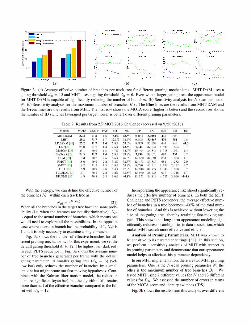
Figure 3. (a) Average effective number of branches per track tree for different pruning mechanisms. MHT-DAM uses agating threshold dth = 12 and MHT uses a gating threshold dth = 6. Even with a larger gating area, the appearance modelfor MHT-DAM is capable of significantly reducing the number of branches. (b) Sensitivity analysis for N -scan parameterN . (c) Sensitivity analysis for the maximum number of branches Bth. The Blue lines are the results from MHT-DAM andthe Green lines are the results from MHT. The first row shows the MOTA score (higher is better) and the second row showsthe number of ID switches (averaged per target, lower is better) over different pruning parameters.

Table 2. Results from 2D MOT 2015 Challenge (accessed on 9/25/2015)

Method MOTA MOTP FAF MT ML FP FN IDS FM Hz

MHT-DAM 32.4 71.8 1.6 16.0% 43.8% 9, 064 32,060 435 826 0.7MHT 29.2 71.7 1.7 12.1% 53.3% 9, 598 33,467 476 781 0.8

LP SSVM [41] 25.2 71.7 1.4 5.8% 53.0% 8, 369 36, 932 646 849 41.3ELP [27] 25.0 71.2 1.3 7.5% 43.8% 7,345 37, 344 1, 396 1, 804 5.7

MotiCon [23] 23.1 70.9 1.8 4.7% 52.0% 10, 404 35, 844 1, 018 1, 061 1.4SegTrack [28] 22.5 71.7 1.4 5.8% 63.9% 7,890 39, 020 697 737 0.2

CEM [29] 19.3 70.7 2.5 8.5% 46.5% 14, 180 34, 591 813 1, 023 1.1RMOT [43] 18.6 69.6 2.2 5.3% 53.3% 12, 473 36, 835 684 1, 282 7.9SMOT [13] 18.2 71.2 1.5 2.8% 54.8% 8, 780 40, 310 1, 148 2, 132 2.7TBD [15] 15.9 70.9 2.6 6.4% 47.9% 14, 943 34, 777 1, 939 1, 963 0.7

TC ODAL [2] 15.1 70.5 2.2 3.2% 55.8% 12, 970 38, 538 637 1, 716 1.7DP NMS [35] 14.5 70.8 2.3 6.0% 40.8% 13, 171 34, 814 4, 537 3, 090 444.8

With the entropy, we can define the effective number ofthe branches Neff within each track tree as:

Neff = eH(Bk). (21)When all the branches in the target tree have the same prob-ability (i.e. when the features are not discriminative), Neffis equal to the actual number of branches, which means onewould need to explore all the possibilities. In the oppositecase where a certain branch has the probability of 1, Neff is1 and it is only necessary to examine a single branch.

Fig. 3a shows the number of effective branches for dif-ferent pruning mechanisms. For this experiment, we set thedefault gating threshold dth to 12. The highest bar (dark red)in each PETS sequence in Fig. 3a shows the average num-ber of tree branches generated per frame with the defaultgating parameter. A smaller gating area (dth = 6) (yel-low bar) only reduces the number of branches by a smallamount but might prune out fast-moving hypotheses. Com-bined with the Kalman filter motion model, the reductionis more significant (cyan bar), but the algorithm still retainsmore than half of the effective branches compared to the fullset with dth = 12.

Incorporating the appearance likelihood significantly re-duces the effective number of branches. In both the MOTChallenge and PETS sequences, the average effective num-ber of branches in a tree becomes ∼50% of the total num-ber of branches. And this is achieved without lowering thesize of the gating area, thereby retaining fast-moving tar-gets. This shows that long-term appearance modeling sig-nificantly reduces the ambiguities in data association, whichmakes MHT search more effective and efficient.

Analysis of Pruning Parameters. MHT was known tobe sensitive to its parameter settings [32]. In this section,we perform a sensitivity analysis of MHT with respect toits pruning parameters and demonstrate that our appearancemodel helps to alleviate this parameter dependency.

In our MHT implementation, there are two MHT pruningparameters. One is the N -scan pruning parameter N , theother is the maximum number of tree branches Bth. Wetested MHT using 7 different values for N and 13 differentvalues for Bth. We assessed the number of errors in termsof the MOTA score and identity switches (IDS).

Fig. 3b shows the results from this analysis over different

N -scan parameters. We fix the maximum number of treebranches to 300, a large enough number so that very fewbranches are pruned when N is large. The results show thatmotion-based MHT is negatively affected when the N -scanparameter is small, while MHT-DAM is much less sensitiveto the parameter change. This demonstrates that appearancefeatures are more effective than motion features in reducingthe number of look-ahead frames that are required to resolvedata association ambiguities. This is intuitive, since manytargets are capable of fast movement over a short time scale,while appearance typically changes more slowly.

Fig. 3c illustrates the change in the MOTA and IDSscores when the maximum number of branches varies from1 to 120. We fix the N -scan pruning parameter to 5 whichis the setting for all other experiments in the paper. Notethat appearance modeling is particularly helpful in prevent-ing identity switches.

5.2. Benchmark Comparison

We test our method on the MOT Challenge benchmarkand the PETS 2009 sequences. The MOT benchmark con-tains 11 training and 11 testing sequences. Users tune theiralgorithms on the training sequences and then submit the re-sults on the testing sequences to the evaluation server. Thisbenchmark is of larger scale and includes more variationsthan the PETS benchmark. Table 2 shows our results on thebenchmark where MHT-DAM outperforms the best previ-ously published method by more than 7% on MOTA. In ad-dition, 16.0% of the tracks are mostly tracked, as comparedto the next competitor at 8.5%. We also achieved the lowestnumber of ID switches by a large margin. This shows the ro-bustness of MHT-DAM over a large variety of videos underdifferent conditions. Also note that because MOT is signifi-cantly more difficult than the PETS dataset, the appearancemodel becomes more important to the performance.

Table 3 demonstrates the performance of MHT andMHT-DAM on the PETS sequences compared to one of thestate-of-the-art tracking algorithms [31]. For a fair com-parison, the detection inputs, ground truth annotations, andevaluation script provided by [31] were used. Our basicMHT implementation already achieves a better or compa-rable result in comparison to [31] for most PETS sequencesand metrics. Cox’s method is also surprisingly close in per-formance to [31] with ∼6% lower MOTA on average withthe exception of the S2L2 sequence where it is∼20% lower.However, considering that Cox’s MHT implementation wasdone almost 20 years ago, and that it can run in real timedue to the efficient implementation (40 FPS on average forPETS), the results from Cox’s method are impressive. Afteradding appearance modeling to MHT, our algorithm MHT-DAM makes fewer ID switches and has higher MOTA andMOTP scores in comparison to previous methods.

6. ConclusionMultiple Hypothesis Tracking solves the multidimen-

sional assignment problem through an efficient breadth-firstsearch process centered around the construction and prun-ing of hypothesis trees. Although it has been a workhorsemethod for multi-target tracking in general, it has largelyfallen out-of-favor for visual tracking. Recent advancesin object detection have provided an opportunity to reha-bilitate the MHT method. Our results demonstrate thata modern formulation of a standard MHT approach canachieve comparable performance to several state-of-the-artmethods on reference datasets. Moreover, an implemen-tation of MHT by Cox [12] from the 1990s comes sur-prisingly close to state-of-the-art performance on 4 out of5 PETS sequences. We have further demonstrated thatthe MHT framework can be extended to include on-linelearned appearance models, resulting in substantial perfor-mance gains. The software and evaluation results are avail-able from our project website.2

Acknowledgments: This work was supported in part by theSimons Foundation award 288028, NSF Expedition award1029679 and NSF IIS award 1320348.

Table 3. Tracking Results on the PETS benchmark

Sequence Method MOTA MOTP MT ML FM IDS

MHT-DAM 92.6% 79.1% 18 0 12 13S2L1 MHT 92.3% 78.8% 18 0 15 17

Cox’s MHT [12] 84.1% 77.5% 17 0 65 45Milan [31] 90.3% 74.3% 18 0 15 22

MHT-DAM 59.2% 61.4% 10 2 162 120S2L2 MHT 57.2% 58.7% 7 1 150 134

Cox’s MHT [12] 38.0% 58.8% 3 8 273 154Milan [31] 58.1% 59.8% 11 1 153 167

MHT-DAM 38.5% 70.8% 9 22 9 8S2L3 MHT 40.8% 67.3% 10 21 19 18

Cox’s MHT [12] 34.8% 66.1% 6 22 65 35Milan [31] 39.8% 65.0% 8 19 22 27

MHT-A+M 62.1% 70.3% 21 9 14 11S1L1-2 MHT-M 61.6% 68.0% 22 12 23 31

Cox’s MHT [12] 52.0% 66.5% 17 14 52 41Milan [31] 60.0% 61.9% 21 11 19 22

MHT-DAM 25.4% 62.2% 3 24 30 25S1L2-1 MHT 24.0% 58.4% 5 23 29 33

Cox’s MHT [12] 22.6% 57.4% 2 23 57 34Milan [31] 29.6% 58.8% 2 21 34 42

References[1] A. Andriyenko, K. Schindler, and S. Roth. Discrete-

continuous optimization for multi-target tracking. In CVPR,2012. 2

[2] S.-H. Bae and K.-J. Yoon. Robust online multi-object track-ing based on tracklet confidence and online discriminativeappearance learning. In CVPR, 2014. 2, 7

2http://cpl.cc.gatech.edu/projects/MHT/

[3] H. Ben Shitrit, J. Berclaz, F. Fleuret, and P. Fua. Multi-commodity network flow for tracking multiple people.PAMI, 2014. 2

[4] J. Berclaz, E. Turetken, F. Fleuret, and P. Fua. Multipleobject tracking using K-shortest paths optimization. PAMI,2011. 2

[5] K. Bernardin and R. Stiefelhagen. Evaluating multiple objecttracking performance: the CLEAR MOT metrics. Image andVideo Processing, 2008. 6

[6] S. Blackman and R. Popoli. Design and Analysis of ModernTracking Systems. Artech House, 1999. 1, 3, 4

[7] M. D. Breitenstein, F. Reichlin, B. Leibe, E. Koller-Meier,and L. V. Gool. Online multiperson tracking-by-detectionfrom a single, uncalibrated camera. PAMI, 2011. 2

[8] W. Brendel, M. Amer, and S. Todorovic. Multiobject track-ing as maximum weight independent set. In CVPR, 2011.2

[9] S. Busygin. A new trust region technique for the maximumweight clique problem. Discrete Appl. Math., 2006. 5

[10] A. Butt and R. Collins. Multi-target tracking by Lagrangianrelaxation to min-cost network flow. In CVPR, 2013. 2, 5

[11] R. T. Collins. Multitarget data association with higher-ordermotion models. In CVPR, 2012. 2

[12] I. J. Cox and S. L. Hingorani. An efficient implementation ofReid’s multiple hypothesis tracking algorithm and its evalu-ation for the purpose of visual tracking. PAMI, 1996. 1, 2, 4,5, 8

[13] C. Dicle, O. Camps, and M. Sznaier. The way they move:Tracking targets with similar appearance. In ICCV, 2013. 7

[14] J. Ferryman and A. Ellis. PETS2010: Dataset and challenge.In AVSS, 2010. 6

[15] A. Geiger, M. Lauer, C. Wojek, C. Stiller, and R. Urtasun. 3Dtraffic scene understanding from movable platforms. PAMI,2014. 7

[16] R. Girshick, J. Donahue, T. Darrell, and J. Malik. Rich fea-ture hierarchies for accurate object detection and semanticsegmentation. In CVPR, 2014. 1, 6

[17] M. Han, W. Xu, H. Tao, and Y. Gong. An algorithm formultiple object trajectory tracking. In CVPR, 2004. 2

[18] C. Huang, Y. Li, and R. Nevatia. Multiple target trackingby learning-based hierarchical association of detection re-sponses. PAMI, 2013. 2

[19] Z. Khan, T. Balch, and F. Dellaert. MCMC-based particlefiltering for tracking a variable number of interacting targets.PAMI, 2005. 2

[20] A. Krizhevsky, I. Sutskever, and G. E. Hinton. Imagenetclassification with deep convolutional neural networks. InNIPS, 2012. 1

[21] C.-H. Kuo, C. Huang, and R. Nevatia. Multi-target track-ing by on-line learned discriminative appearance models. InCVPR, 2010. 2

[22] C.-H. Kuo and R. Nevatia. How does person identity recog-nition help multi-person tracking? In CVPR, 2011. 2

[23] L. Leal-Taixe, M. Fenzi, A. Kuznetsova, B. Rosenhahn, andS. Savarese. Learning an image-based motion context formultiple people tracking. In CVPR, 2014. 7

[24] L. Leal-Taixe, A. Milan, I. Reid, S. Roth, and K. Schindler.MOTChallenge 2015: Towards a benchmark for multi-targettracking. arXiv:1504.01942 [cs], 2015. 6

[25] F. Li, T. Kim, A. Humayun, D. Tsai, and J. M. Rehg. Video

segmentation by tracking many figure-ground segments. InICCV, 2013. 1, 5

[26] J. Liu, P. Carr, R. T. Collins, and Y. Liu. Tracking sportsplayers with context-conditioned motion models. In CVPR,2013. 2

[27] N. McLaughlin, J. Martinez Del Rincon, and P. Miller.Enhancing linear programming with motion modeling formulti-target tracking. In WACV, 2015. 7

[28] A. Milan, L. Leal-Taixe, I. Reid, and K. Schindler. Jointtracking and segmentation of multiple targets. In CVPR,2015. 7

[29] A. Milan, S. Roth, and K. Schindler. Continuous energy min-imization for multitarget tracking. PAMI, 2014. 7

[30] A. Milan, K. Schindler, and S. Roth. Challenges of groundtruth evaluation of multi-target tracking. In CVPR Workshop,2013. 6

[31] A. Milan, K. Schindler, and S. Roth. Detection-andtrajectory-level exclusion in multiple object tracking. InCVPR, 2013. 6, 8

[32] S. Oh, S. Russell, and S. Sastry. Markov Chain Monte Carlodata association for multi-target tracking. IEEE Transactionson Automatic Control, 2009. 2, 6, 7

[33] P. R. Ostergard. A new algorithm for the maximum-weightclique problem. Nordic Journal of Computing, 2001. 5

[34] D. J. Papageorgiou and M. R. Salpukas. The maximumweight independent set problem for data association in multi-ple hypothesis tracking. Optimization and Cooperative Con-trol Strategies, 2009. 2, 4

[35] H. Pirsiavash, D. Ramanan, and C. C. Fowlkes. Globally-optimal greedy algorithms for tracking a variable number ofobjects. In CVPR, 2011. 2, 7

[36] D. Reid. An algorithm for tracking multiple targets. IEEETransactions on Automatic Control, 1979. 1, 2

[37] A. Segal and I. Reid. Latent data association: Bayesianmodel selection for multi-target tracking. In ICCV, 2013.2, 5

[38] H. B. Shitrit, J. Berclaz, F. Fleuret, and P. Fua. Tracking mul-tiple people under global appearance constraints. In ICCV,2011. 2

[39] A. Smeulder, D. Chu, R. Cucchiara, S. Calderara,A. Deghan, and M. Shah. Visual tracking: An experimen-tal survey. PAMI, 2014. 2

[40] X. Song, J. Cui, H. Zha, and H. Zhao. Vision-based multipleinteracting targets tracking via on-line supervised learning.In ECCV, 2008. 2

[41] S. Wang and F. C. Learning optimal parameters for multi-target tracking. In BMVC, 2015. 7

[42] B. Yang and R. Nevatia. An online learned CRF model formulti-target tracking. In CVPR, 2012. 2

[43] J. Yoon, H. Yang, J. Lim, and K. Yoon. Bayesian multi-object tracking using motion context from multiple objects.In WACV, 2015. 7

[44] A. R. Zamir, A. Dehghan, and M. Shah. GMCP-tracker:Global multi-object tracking using generalized minimumclique graphs. In ECCV, 2012. 5

[45] L. Zhang and R. Nevatia. Global data association for multi-object tracking using network flows. In CVPR, 2008. 2