DOCID: 3838688 SECRET

Multiple Hypothesis Testing and the Bayes Factor*

BY_l ____ I Secret

Derives some of the main properties of the Bayes Factor and its logarithm and discusses the application of these properties to the classical "two disjoint hypotheses" situation, and-more importantly­to the situation of N hypotheses, n of which are true where n < < N. The object is to reject as many untrue hypotheses as possible while accepting a reasonable percentage of correct hypotheses. Gives two examples of the N hypotheses situation which are of COMSEC (and possibly also general) interest.

In this paper we derive some of the main properties of the Bayes fac­tor and its logarithm in a context which applies to many Agency statis­tical problems. The Bayes factor arises naturally as a result of an ap­plication of the fundamental Neymann-Pearson Lemma of classical hypothesis testing theory. With the "two hypotheses" theory in mind we consider the more important situation of N hypotheses, n of which are true with n < < N. Finally, we discuss two examples of the N hypotheses situation which are of considerable COM SEC interest.

1. Consider a list

Z = z,, ... , Zr

of random variables defined on a finite sample space E, an arbitrary member of which is denoted

e = e1, ... , er.

Suppose we have two (disjoint) hypotheses H, and H2 about the list such that each hypothesis completely determines the probability law of Z (denoted Pi and P2, respectively). (This is not quite the way the world is around here. This will be discussed later). For notational ease, we write P;(e) for P;(Z = e), i = 1, 2.

NSAL-S-193,398

- 6R9UP I -EiCIUded llUW autvwatic llew•pading ·nd dec:l15:riftption.

63 S~CR~T

P.L. 86-36

::)eclassifi ed and approved for ·elease bv f\JSA on '10-29-2009 :iursuantto E i::) 12958, as rirnended

P.L. 86 - 36

D.Q._CID: 3838688 S~ HYPOTHESIS TESTING

The problem is to decide which hypothesis is true. The celebrated Neymann-Pearson Lemma tells us how to proceed. If we set

P1 (reject H1 ) = a

P2 (accept H1) = b

and fix a with the hope of minimizing b, our hopes will be realized if we perform a test of the following kind:

. Pi (e) Accept H1 if-- ~ c

Pz(e)

. . Pi (e) ReJect H1 if-(-) < c,

P2 e

where e is the observation we are presented with and c is a constant to be determined. This is intuitively quite reasonable. It simply says to accept Hi if the probability of the observation when H1 is true is sufficiently greater than the probability of the observation when H2 is true. The proof is just about this simple. See reference ( 1 J. Actually, if f is any real valued increasing function, then an equivalent procedure is:

. [ P1 (e)J Accept H1 if f --) Pde

~ f (c)

Reject H1 if f [ Pi(e)J < f (c). P2 (e)

The quantity

B(e) = P1 (e)/P2 (e)

is termed the factor, or the Bayes factor, in favor of H1 over H2. It is often convenient to take for the f above, the natural logarithm ln. The terminology is:

L(e) = ln [P1 (e)/P2 (e)]

is the log factor or Bayes score in favor of Hi over H2. Note that no assumptions about Z (normality, independence, etc.)

have been made. Still, it is possible to obtain some interesting results about B and L.

First, note that if e is regarded as an arbitrary point in the. sample space rather than a fixed observation, both B and L can be considered random variables. Since

a =Pi (B < c)

b = P2(B ~ c),

64

- - ·---------------""'

DOCID: 3838688 I~------.

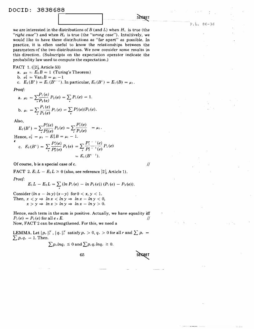
we are interested in the distributions of B (and L) when H1 is true (the "right case") and when H2 is true (the "wrong case"). Intuitively, we would like to have these distributions as "far apart" as possible. In practice, it is often useful to know the relationships between the parameters of the two distributions. We now consider some results in this direction. (Subscripts on the expectation operator indicate the probability law used to compute the expectation.)

FACT 1. ([2], Article 53) a. µ.2 == E2 B = 1 (Turing's Theorem) b. u~ =Var2B=µ.1-l c. E2 (B") = E1 (B" - 1

) . In particular, E2 (B;) = E1 (B) = µ1 .

Proof: Pi (e)

a. µ2 = 2:-- P2(e) = l:P1(e) = 1. , P2 (e) ,

b. µ1 = L Pi(e) P1 (e) = L Pi (e)IP2 (e) . • P2(e) ,

Also, ; Pi(e) Pi (e)

EdB ) = ~P~(e) Pi(e) = ~P2(e)

Hence, u~ = µ1 - E~B = µ1 - 1.

'

Of course, bis a special case of c.

FACT 2. E1 L - E2 L 2 0 (also, see reference [2 ], Article 1).

Proof: E1L - E2L = L(lnPi(e) - lnPi(e)) (P1(e) - Pde)).

Consider (ln x - lny) (x-y) for 0 < x, y < 1. Then, x < y ~ ln x < ln y ~ ln x - ln y < 0,

x > y ==;:> ln x > ln y ~ ln x - ln y > 0.

II

Hence, each term in the sum is positive. Actually, we have equality iff P1 (e) = P2 (e) for all et E. II Now, FACT 2 can be strengthened. For this, we need a

LEMMA. Let \p, If, I q, If satisfy p, > 0, q, > 0 for all rand L p, LPrQr = 1. Then.

_Lp,lnq, ::; 0 andLp,q,lnq, 2 0.

65

DQ...CID: 3838688 S~ HYPOTHESIS TESTING

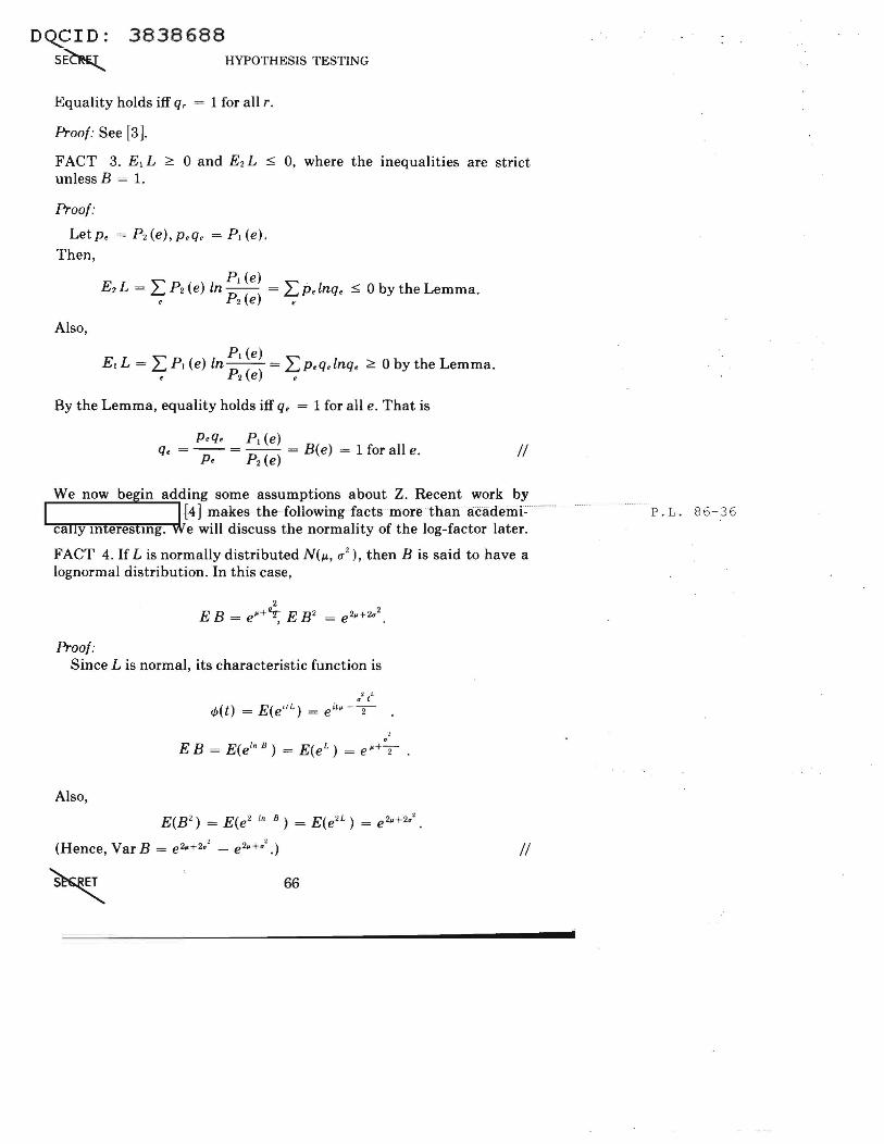
Equality holds iff q, = 1 for all r.

Proof: See [3 ].

FACT 3. E1 L ~ 0 and E z L ::;; 0, where the inequalities are strict unless B = 1.

Proof:

Letp. = P2(e),p,q, = P 1 (e) .

Then,

P1 (e) EzL = L Pz(e) ln-- = _Lp. lnq. ::;; 0 by the Lemma.

• P 2(e) ,

Also,

Pi(e) E1 L = L P1 (e) ln-- = L.p.q, lnq. ~ 0 by the Lemma.

• P2 (e) •

By the Lemma, equality holds iff q, = 1 for all e. That is

p . q. P1 (e) q. = -- = -- = B(e) = 1 for all e.

p . Pz(e) II

We now be in adding some assumptions about Z. Recent work by [4]···makes ·· the ··foHowing ··facts ···more ·· tha.n··· a.cademi~ ·· ··­

....,,.,ca,,.,.,.,,y.,..,1""'n""e""'r'""'e""'s """1n""'g""".""""" 1e will discuss the normality of the log-factor later.

FACT 4. If Lis normally distributed N(µ., ,,z ), then B is said to have a lognormal distribution. In this case,

2

EB = e"+~ E B 2 = e 2-+ 2•2

Proof: Since L is normal, its characteristic function is

"J. :l. 0 t

<t>(t) = E(e'' L) = ei1• - - 2-

' EB = E(e1

" 8

) = E(e l ) = e"+T .

Also,

E(B2) = E(e2 1

" 8

) = E(en ) = e :i..+2.' .

(Hence, Var B = ez..+2.' - e 2•+-' .) II

~ 66

P . L . 86 - 36

DOCID: 3838688

.___ __ ____.I u ~ ... ..

DEFINITION. Let X be a random variable and </lx (t) E(e"x ) its characteristic function. Then the n'h cumulant of X, K. (X), is defined by (if it exists)

K. (X) = i - ":£.____ (ln </lx (t))/1 - o. dt"

For example,

K1 (X) = i - i !!_(ln </lx (t))/ r-o = i- i !!_(E(e i•X ))I 1=0

dt dt

= i- i E(i X e'1x )/ 1~0 =EX.

Similarly, [5],

E X 2 = K z (X) + Kf(X) (i.e., Var X = Kz(X))

E X J = K3 (X) + 3K2 (X) Ki (X) +Kt (X), etc.

Also, by definition, the expansion for in <Px (t) is

ln </lx (t) = L K.(X) (it) ' /k! k = i

These ideas lead to the following important

FACT 5. [6]. The cumulants of the distribution of L satisfy

K2 KJ K4 K1 - 2! + 3! - 4! + . . . = 0 if Hi is true, and

K z K3 K1 + 2! + 3! + . . . = 0 if H2 is true.

Proof: In the right case,

" { . Pi (e)} <P1 (t) = ~Pi (e) exp Lt in -- . , P2 (e)

Hence, . " P2 (e)

<P1 (i) = ~ P1 (e)-p ( ) = L Pz(e) = 1. e I e e

Now,

in q,i(t) = L K, ·(it)* /k!. k-1

67

P . L. 86- 36

DOCID: 3838688

~ HYPOTHESIS TESTING

From the expression above for </>1 (i), we have

k - I

A similar proof works for the wrong case (and for continuous distri­butions). II FACT 6. If Xis a normal random variable, then K. (X) = 0 for n > 2.

Proof: ln </>x (t) = i µ. t - u

2

t2

• II 2

FACT 7. If L is normally distributed N(µ.1, ui) in the right case and N(µ.2, u~) in the wrong case, then

ui = 2µ.1 and u~ = - 2µ.2 .

Proof: This follows immediately from the preceding two facts; however, we give the following proof (which does not require the introduction of the concept of cumulant): UnderH1,

</>L (t) = E(e;L')

{ . [P1(e)]} = L Pi (e) exp it ln --• Pde)

Hence,

. '""' Pde) </>L (i) = .t...., P1 (e)-- = 1 • P1 (e)

Also,

Hence,

ln(l) = 0 = ln <f>i (i) = -µ1 + ui/2

Hence,

Similarly, under H2,

. P1 (e) <J>d-i) = L Pde)--= 1, and

• Pde)

L ""' N(µ.2 , u~) =

2 2 2 . . •2(-i) •o

( ") P2'(-1)--2- P2+2

</>i -i = e = e

s~ 68

DOCID: 3838688

Hence,

Hence,

II

FACT 8. Let L "' N(µ1, ui) in the right case and N(µz, u~) in the wrong case. Then:

a. E, L = 112 ln(E, B). b. ui = ll3 ln(E1 B 2

).

c. u~ = ln(E2 B 2) = ln(E, B).

Proof:

b. ln(E1 B 2) = ln(eZi<• +z.f) = ui + 2ui = 3ui.

II

Definition: If L "' N(µ1, ui) in the right case and L ,..._, N(µz, ui) in the wrong case, then the sigma-age S = (µ1 - µz )lu2.

FACT 9. Under the conditions of the above definition, a. µ1 = 112 ln(E, B) b. ui = ln(E1 B) c. µ2 = - 112 ln(E, B) d. u~ = ln(E, B) e. S = Vln(E, B)

Proof: Sections a-d under FACT 9 follow from FACTS 7 and 8.

112 ln(E, B) - ( -112 ln(E, B)) S = (µ1 - µz )lu2

yln(E, B)

=yfln(E, B) II This fact says that if L is normal, calculation of E, B determines both right and wrong case distributions of L. Finally, we note the following relations between expected scores and the concept of entropy:

p, (e) E,L =,LP, (e) ln -- =LP, (e) lnP, (e) - ,LP, (e) lnPz(e)

• Pz(e) • •

= -H, (Z) - L P1 (e) ln P2 (e) •

69

P.L. 86-36

DOCID: 3838688

~ HYPOTHESIS TESTING

where Hi (Z) is the entropy of Z assuming that Hi is true. Similarly,

If the size of the sample space is N, and P2 (e) = ~for all et E, then, . N EiL = - Hi (Z) + lnN

1 E 2L = lnN +-ElnPi(e) .

N. Hence,

H1(Z) = lnN- E1L.

2. It has already been remarked that the situation of two simple hypotheses is somewhat unreal from our point of view. A situation closer to reality is the following. We have a random list Z = Z 1 , ••• , Zr defined on a sample space E, an arbitrary member of which is denoted e = e1, . .. , er. We have N hypotheses H1, ... , HN about Z with n of them being true, where 1 < n < < N. We assume that each H i deter­mines two probability laws P; and P _ i for Z:

P ;(e) = P(Z=el Hi is true) p _i(e) = P(Z=e I Hi is not true).

(In many COMSEC applications, it is intuitively reasonable to take P _; to be the same for all i.) We want to eliminate as many wrong hypotheses as possible while accepting a reasonable fraction of correct hypotheses. To accomplish this, we test each Hi against -H; using the theory of the preceding section. That is, we form

L; = lnjPi(e)/P_i(e) ).

If we can assume that Li is normally distributed m both right and wrong cases, then from FACT 9, there exists

Then,

µi > 0 such that with ul = 2µ. i , Li "' N(µ i, ul ) if Hi is true and Li "' N(-µi, ut) if Hi is not true.

(Ci - (-µd)

P (accept Hi I -Hi) = 1 - F Ui

P(reject H i I Hi)= F (Ci Ui- µJ = a;,

70

DOCID: 38386~------.

I where Fis the N(O, 1) distribution function and c; is the threshold for the test (the c which appears in the statement of the Neymann-Pear­son Lemma). We fix a; = a (the same a for all i) and can then solve for the c; above. Then the theory of section 1 indicates that we have minimized b; given the fixed value a. In particular, if we take a = 1/2, as is often done, then c; = µ; and b; depends upon

µ; - (-µ;)

<Ti

which is the sigma-age as defined in section 1. It is this appearance of the sigma-age which makes the concept important.

Now, after testing all of the hypotheses H; as above, the expected number of wrong hypotheses ["Expected Wrong Case Survivors," E(WCS)] accepted is (since we assume n < < N)

N

E(WCS) ~ Lb; i- l

and the expected number of correct hypotheses ["Expected Right Case Survivors," E(RCS)] accepted is

E(RCS) =an.

Now, in order to determine E(WCS) as above, it is necessary to deter­mine all of the b;'s and sum them. This would cost almost as much as doing the actual testing of the hypotheses. Hence, from a COMSEC point of view, the above expression for E(WCS) is not practically use­ful. We need another method to estimate E(WCS). The method usually employed is as follows (for simplicity, assume we have fixed a= 1/2). We find an approximationµ to the average of the µ;'s

1 N

µ. =-.L µ;. N;-1

Then we form

b = 1-F(µ~µ0

and take as an estimate to E(WCS)

E(WCS) ~Nb.

In general, let µ; = E;L; denote the expected value of L; computed assuming that H; is true, and µ. _ ; = E _ ;L; the expected value com­puted assuming H; is not true. Similarly for u2- ; = Var_ ;L;. Then the quantity

IE(µ;) - E(µ_ ;) IJVE(u2- ;)

71

P. L. 86-36-

DOCID: 3838688 ~ HYPOTHESIS TESTING

is some sort of approximation to an expected sigma-age. We call it the essential sigma-age. The procedure is quite questionable, and there seems to be room for considerable investigation, theoretical and em­pirical, in this area. In the examples of section 4, we indicate how to determine the approximationµ.

3. In this section, we say the little that it seems to be possible to say about normality of the log factor. Normality of L is often assumed in general due to the fact that, in practice, it often turns out that B is a product of random variables. Then L is a sum of random variables, and if these random variables may be assumed to be independent and identically distributed with finite variances, then a central limit theorem will imply the approximate normality of L (see reference [5] page 431, Theorem 4A). Actually, less stringent requirements may be made of the random variables and normality in the limit may still be imolied (a!!ain see reference rsl oa!!e 431 Theorem 4B).

72

I////

EO 1. 4. ·(c) P.L. 86-36

EO 1. 4. ( c) P.L. 86-36

DOCID: 383868~8~-----,I

I .

73

1'

P.L. 86-36

1. 4. ( c)

P.L. 86-36

DOCID: 3838688

- SECl':ET- HYPOTHESIS TESTING

SECRET 74

I

1. 4. ( c)

P.L. 86-36

DOCID: 38386~------, I

75

~~::. ······························

··· ·········· ········ J~~

. ~ · .............. ··· ·········· ·· P . 1 . 86 - 36

EO 1 . 4 . ( c)

P.L. 86-36

DOCID: 3838688 SECRET HYPOTHESIS TESTING

76

1. 4. ( c) P.L. 86-36

DOCID: 383868~-------. P.L, 86-.36

I see RE+-

I

77 SEERl!T

DOCID: 3838688 SECRl!T HYPOTHESIS TESTING

78

I .

' EO 1. 4. ( c) I P.L. 86-36

DOCID: 3838688

I

79

sl!!ern:r P.L. 86-36

EO 1. 4. ( c) P.L. 86-36

DOCID: 3838688 SECRI:+ HYPOTHESIS TESTING

REFERENCES

[ l] Hogg and Craig, Introduction to Mathematical Statistics (2nd ed ., The Macmillan Co., New York, 1965).

[ 2 J Collected Papers on Mathematical Cryptology.

[ 3 J Hardy, Littlewood and Poly a , Inequalities (Cambridge University Pre.ss,Jf)i37} . ..

[ 4] , "The Sfre.llgth of the Bayes Score, SJ2 /nfor~ ._m_a-l'"'N,..o-t-e""'#""'283~'"'(""8"'S-ep_t_e_m..,.b_e_r ""197~0.,..) .---'

[5] Parzen , Modern Probability Theory and Its Applications (John Wiley and Sons, Inc ., New York, 1960) .

[ 6J Good and Toulmin, "Coding Theorems and Weight of Evidence," Jour. Inst. Maths Applies, 4 (1968), 94-105.

l 7JI I [8]...__. _______ .......

SEeR~T 80

I/

EO 1 . 4 . ( c.) P.L. 86-36

P.L. 86 - 36

EO L 4 . (c)

P,L. 86 - 36