multiphase performance validation
TRANSCRIPT

Multiphase performance validation
Halfdan Rognes Knudsen
Master of Energy and Environmental Engineering
Supervisor: Lars Erik Bakken, EPT
Department of Energy and Process Engineering
Submission date: June 2013
Norwegian University of Science and Technology


I
Abstract
The oil and gas industry wishes to further develop multi-phase technology in order to reduce con-
struction costs and increase production from existing fields. Both suppliers and operators are in-
vesting in development of subsea equipment. The goal is to reduce environmental impact and
energy costs.
Suppliers are extending their product portfolio with wet gas compressors or high GVF multi-
phase pumps. Accurate predictions of performance are important to the customer, as the customer
needs the predictions in order to estimate return of investments, and for designing the overall
production plant.
Well-established models for predicting performance of single-phase and liquid dominated two-
phase flow exists. But companies aim to extend these models, in order to also predict perfor-
mance of gas dominated flow.
Based on literature study and available test data, the goal is to establish reliable routines on two-
phase performance calculations. This includes solving challenges related to both calculations and
measurements.
A laboratory rig have been planned in order to validate different temperature sensors ability to
measure in two phase flow. Main focus has been on generating conditions where thermal equilib-
rium is absent. Different solutions on how to generate non thermal equilibrium two-phase mix-
tures have been presented. Relevant temperature sensors have been chosen and a sensitivity anal-
ysis has been performed to make sure they are accurate enough for the assignment. Solutions to
challenges like gas phase humidity and local gas phase temperature measurements are presented.
In the end a complete procedure on how to perform the tests is suggested.
This thesis aimed to validate the functionality of a Direct Integration method implemented in the
process simulation tool HYSYS. Trough different examples it has been compared to Shultz and a
Matlab implementation of the Direct Integration model presented in this thesis. The HYSYS im-
plementation was found to differ from the original Direct Integration method presented by Hun-
tington. For polytrophic efficiency calculations it does not seem to be implemented at all. If the
Direct Integration method is to be used in performance calculations, better results will be
achieved by applying the Matlab implementation presented in this thesis.
Industry actors sometimes reduce analysis costs by neglecting heavier parts of the composition.
The importance of knowing the exact fluid composition is discussed in this thesis. Results from
simulations where heavier components are neglected are presented. It has been found that the
accuracy of the performance calculations is highly dependent on the accuracy of the composition.
The calculations of polytrophic efficiency are especially sensitive when operating far into the
two-phase area.

II

III
Sammendrag
Olje og gass industrien ønsker å videreutvikle flerfase trykkøknings teknologi, for å redusere
byggekostnader og for å øke produksjonen fra eksisterende felt. Både leverandører og operatører
investerer i utviklingen av Subsea-utstyr og konsekvensene er redusert miljøpåvirkning og ener-
giforbruk.
Flere leverandører utvider sin produktportefølje med våtgass kompressorer eller flerfasepumper.
Nøyaktige beregninger av ytelse er viktig for kundene, ettersom kundene trenger beregningene
for å estimere lønnsomheten av sine investeringer, og for å dimensjonere et omliggende produk-
sjonsanlegg.
Veletablerte og aksepterte modeller for prediksjon av ren væske ytelse og væskedominert tofase
ytelse eksisterer. Men selskapene ønsker å utvide disse modellene, slik at de også kan bli brukt til
å prediktere ytelse ved gass dominert strømning.
Basert på litteraturstudier og tilgjengelige testdata, er målet å etablere pålitelige rutiner for tofase
prediksjon. Utfordringer knyttet til både beregninger og målinger er behandlet i denne oppgaven.
En laboratorierigg har blitt planlagt. Hensikten er å validere forskjellige temperatur sensorers
evne til å gjøre pålitelige målinger i to fase strømnings regime. Hovedfokus har vært på å genere-
re forhold der termisklikevekt er fraværende. Ulike løsninger på hvordan gas og væske kan mik-
ses for å generere en temperaturforskjell mellom fasene, er presentert i oppgaven. Relevante tem-
peratursensorer er valgt ut, og en sensitivitetsanalyse er utført for å sørge for at sensorene er nøy-
aktige nok. Utfordringer som gassfuktighet og lokale gass temperaturmålinger blir grundig gjen-
nomgått. Til slutt blir det foreslått en fullstendig test prosedyre.
Denne oppgaven har forsøkt å validere funksjonaliteten til Direkte Integrasjon i prosess simule-
ringsverktøyet HYSYS. Gjennom forskjellige eksempler har Direkte Integrasjon i HYSYS blitt
sammenlignet med Shultz og en implementering av Direkte Integrasjon i Matlab. Matlab imple-
menteringen er presentert i denne oppgaven. Det har vist seg at Directe Integrasjon i HYSYS
avviker fra den opprinnelige Direkte Integrasjons metoden presentert av Huntington. For bereg-
ning av polytropisk virkningsgrad ser det ut til at Direkte Integrasjon ikke er implementert i det
hele tatt. Hvis det er ønskelig å benytte Direkte Integrasjon i fremtidige ytelses beregninger, vil
man oppnå bedre resultat om man benytter Matlab modellen som blir presentert i denne oppga-
ven.
Aktører i Industrien forsøker noen ganger å redusere kostnader ved å neglisjere de tyngste fluid
komponentene. Viktigheten av å kjenne til den nøyaktige fluid komposisjonen diskuteres i denne
oppgave. Resultater fra simuleringer der tyngre komponenter er neglisjert viser at nøyaktigheten
av ytelses beregninger er svært avhengig av nøyaktigheten av sammensetningen. Det ble også
funnet at beregningene av polytropisk virkningsgrad er spesielt sensitive når det opereres i tofase
området.

IV

V
Acknowledgements
This Master Thesis is performed at the Department of Energy and Process Engineering at the
Norwegian University of Science and Technology, during spring 2013.
I would like to thank my supervisor Professor Lars Erik Bakken and my fellow students at the
study hall, for their important inputs.
Trondheim 19. December 2012
Halfdan Rognes Knudsen

VI
VII
Table of Contents
FIGURES ....................................................................................................................................... 2
TABLES ......................................................................................................................................... 4
ROMAN SYMBOLS ..................................................................................................................... 6
GREEK SYMBOLS ...................................................................................................................... 7
SUBSCRIPTS ................................................................................................................................ 7
ABBREVIATIONS ....................................................................................................................... 8
1 INTRODUCTION ............................................................................................................. 10
1.1 Background ......................................................................................................................... 10
1.2 Objective ............................................................................................................................. 10
1.3 Approach ............................................................................................................................. 12
2 MULTI-PHASE FLOW THEORY ................................................................................. 14
2.1 Simple definitions ............................................................................................................... 14
2.2 Flow regimes ....................................................................................................................... 15
2.3 Mixed flow model ............................................................................................................... 15
2.4 Two-fluid model ................................................................................................................. 16
3 SINGLE-PHASE PUMP THEORY ................................................................................ 18
3.1 Affinity laws ....................................................................................................................... 20
3.2 Viscosity.............................................................................................................................. 21
4 MULTI-PHASE PUMP THEORY .................................................................................. 24
4.1 Affinity and Similarity laws ................................................................................................ 24
4.2 Two-phase multipliers......................................................................................................... 25
4.2.1 Analytical approach ................................................................................................ 26
4.2.2 MIT-model.............................................................................................................. 26
VIII
4.3 Gas compression ................................................................................................................. 27
4.3.1 Isothermal compression .......................................................................................... 27
4.3.2 Polytrophic compression ........................................................................................ 28
4.4 Viscosity.............................................................................................................................. 30
4.5 Phase transition ................................................................................................................... 31
5 TEMPERATURE MEASUREMENTS .......................................................................... 34
5.1 Accuracy ............................................................................................................................. 34
5.2 Sensor technologies............................................................................................................. 36
5.2.1 Thermocouples ....................................................................................................... 36
5.2.2 Resistance temperature detectors (RTD) ................................................................ 37
5.2.3 Thermistors ............................................................................................................. 37
5.2.4 Pyrometers .............................................................................................................. 38
5.3 Two-phase temperature measurements ............................................................................... 38
6 LABORATORY RIG ....................................................................................................... 42
6.1 Conditions and setup ........................................................................................................... 43
6.2 Engineering ......................................................................................................................... 44
6.2.1 Temperature measurements .................................................................................... 45
6.2.2 Test section ............................................................................................................. 46
6.2.3 Gas phase humidity ................................................................................................ 50
6.2.4 Gas volume fraction ................................................................................................ 52
6.2.5 Generating liquid dominated flow .......................................................................... 52
6.2.6 Generating gas dominated flow .............................................................................. 54
6.3 Test procedure ..................................................................................................................... 56
6.4 Sources of Error .................................................................................................................. 58
7 VALIDATION OF DIRECT INTEGRATION IN HYSYS .......................................... 60
7.1 Direct Integration ................................................................................................................ 60
7.2 Implementation of direct integration in HYSYS ................................................................ 61
7.3 Implementation of direct integration in Matlab .................................................................. 63
7.3.1 DirectIntegrationT() ................................................................................................ 63

IX
7.3.2 DirectIntegrationEtha() ........................................................................................... 64
7.4 Validation ............................................................................................................................ 65
8 INFLUENCE OF HEAVY COMPONENTS ON THE PERFORMANCE
CALCULATIONS ....................................................................................................................... 68
8.1 Compositions ...................................................................................................................... 68
8.2 Compression path and performance parameters ................................................................. 70
9 CONCLUSIONS AND SUGGESTIONS TO FURTHER WORK .............................. 74
REFERENCES ............................................................................................................................ 76
APPENDIX .................................................................................................................................. 80
A - OFFER ON THERMO-NEEDLE-PROBE SYSTEM ....................................................... 82
B - DATA SHEETS ..................................................................................................................... 84
C - LIQUID DOMINATED MIXER CALCULATIONS ........................................................ 92
D - SIMULATION ENVIRONMENT TEST RIG ................................................................... 94
E - MATLAB IMPLEMENTATION OF DIRECT INTEGRATION ................................... 96
F - COMPLETE DIRECT INTEGRATION RESULTS....................................................... 102

1
2
Figures
Figure 1 Boosted production compared to natural production. ...................................................... 10
Figure 2 Gas-liquid flow regime in horizontal pipes [ 3 ]. ............................................................. 15
Figure 3 Velocity diagrams of a centrifugal impeller. ................................................................... 18
Figure 4 Velocity diagram at impeller inlet. .................................................................................. 18
Figure 5 Velocity diagram at impeller outlet. ................................................................................ 19
Figure 6 Pump characteristics with specified losses. ..................................................................... 19
Figure 7: Correction of head and efficiency [ 2 ]. .......................................................................... 21
Figure 8 Phase envelope of a typical hydrocarbon......................................................................... 32
Figure 9 Temperature sensitivity analysis, with an inaccuracy of 0.2 K. ...................................... 35
Figure 10 Temperature sensitivity analysis, with an inaccuracy of 0.002 K. ................................ 36
Figure 11 Comparison of RTDs, NTC thermistors and Thermo couples. ..................................... 38
Figure 12 Temperature and conductivity measurement of a passing bobble [ 27 ]. ...................... 39
Figure 13 Simple drawing of the test rig. ....................................................................................... 42
Figure 14 Heater and saturator simulations. ................................................................................... 44
Figure 15 Concept number one - CTC probe setup. ...................................................................... 47
Figure 16 Concept number two - PT100 RTD shield setup. .......................................................... 48
Figure 17 Concept number three - PT100 Gas suction setup. ........................................................ 49
Figure 18 Saturation example ........................................................................................................ 51
Figure 19 Perforated tube in mixer................................................................................................. 53
Figure 20 Nozzle mounting. ........................................................................................................... 55
Figure 21 HYSYS test procedure simulations ............................................................................... 57
Figure 22 HYSYS compressor calculation options ........................................................................ 60
Figure 23 DirectIntegrationT() first step iteration .......................................................................... 63
Figure 24 DirectIntegrationT() after last step iteration .................................................................. 64
Figure 25 DirectIntegrationEtha() .................................................................................................. 65
Figure 26 Direct integration, Composition A VS B, Number of steps = 10, GVF 90%. ............... 71
Figure 27 Direct integration, Composition A VS B, Number of steps = 10, GVF 60%. ............... 72
Figure 28 Direct integration, Composition A VS B, Number of steps = 10, GVF 30%. ............... 72
Figure 29 Direct integration, Composition A VS B, Number of steps = 10, GVF 0%. ................. 73
Figure 30 Direct integration, Composition A VS B, Number of steps = 10, GVF 0% ............... 103

3
Figure 31 Direct integration, Composition A VS B, Number of steps = 10, GVF 10%. ............. 103
Figure 32 Direct integration, Composition A VS B, Number of steps = 10, GVF 20%. ............. 104
Figure 33 Direct integration, Composition A VS B, Number of steps = 10, GVF 30%. ............. 104
Figure 34 Direct integration, Composition A VS B, Number of steps = 10, GVF 40%. ............. 104
Figure 35 Direct integration, Composition A VS B, Number of steps = 10, GVF 50%. ............. 105
Figure 36 Direct integration, Composition A VS B, Number of steps = 10, GVF 60%. ............. 105
Figure 37 Direct integration, Composition A VS B, Number of steps = 10, GVF 70%. ............. 105
Figure 38 Direct integration, Composition A VS B, Number of steps = 10, GVF 80% .............. 106
Figure 39 Direct integration, Composition A VS B, Number of steps = 10, GVF 90%. ............. 106

4
Tables
Table 1 Temperature measurement sensitivity analysis ................................................................. 34
Table 2 Fluid conditions 2 .............................................................................................................. 43
Table 3 Temperature sensor data ................................................................................................... 46
Table 4 Sensitivity of liquid temperature measurements on gas temperature calculations............ 46
Table 5 Fluid conditions ................................................................................................................. 47
Table 6 Effect of condensation on GVF ......................................................................................... 52
Table 7 Perforated tube Flow rate/Pressure calculations ............................................................... 53
Table 8 Nozzle GVF calculations option 1 .................................................................................... 54
Table 9 Nozzle GVF calculations option 2 .................................................................................... 55
Table 10 Conditions ....................................................................................................................... 62
Table 11 Outlet temperature calculations ....................................................................................... 62
Table 12 Conditions ....................................................................................................................... 62
Table 13 Polytrophic efficiency calculations ................................................................................. 62
Table 14 Conditions ....................................................................................................................... 66
Table 15 Outlet temperature calculations of a hydrocarbon mixture at 60% GVF ........................ 66
Table 16 Outlet temperature calculations of water ........................................................................ 67
Table 17 Hydrocarbon composition Actual mixtures VS Low cost analyzes ................................ 69
Table 18 Imagined test results ........................................................................................................ 70
Table 19 Performance Calculations ............................................................................................... 70
Table 20 Direct Integration results 90%-60%GVF ...................................................................... 102
Table 21 Direct Integration results 50%-20%GVF ...................................................................... 102
Table 22 Direct Integration results 10%-0%GVF ........................................................................ 103

5
6
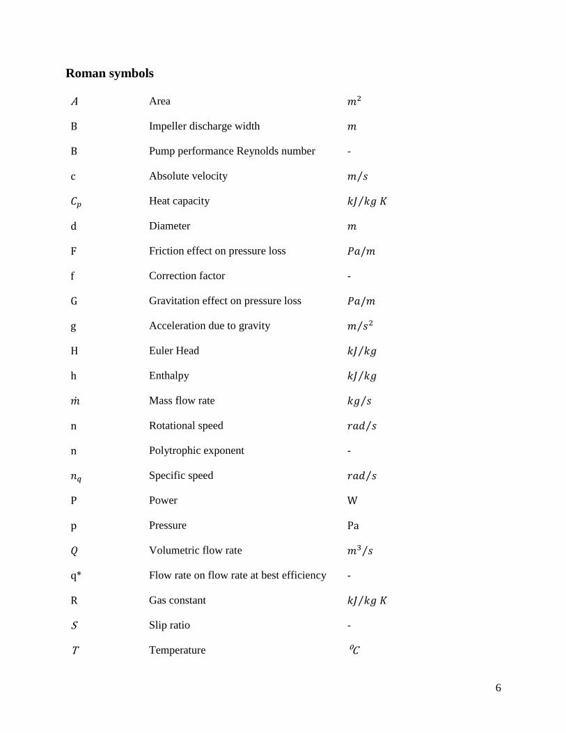
Roman symbols
A Area
B Impeller discharge width
B Pump performance Reynolds number -
c Absolute velocity
Heat capacity
d Diameter
F Friction effect on pressure loss
f Correction factor -
G Gravitation effect on pressure loss
g Acceleration due to gravity
H Euler Head
h Enthalpy
Mass flow rate
n Rotational speed
n Polytrophic exponent -
Specific speed
P Power W
p Pressure Pa
Volumetric flow rate
q* Flow rate on flow rate at best efficiency -
R Gas constant
S Slip ratio -
T Temperature ⁰C

7
u Circumferential velocity
v Specific volume
v Relative velocity
X Compressibility function -
x Axial distance m
Y Compressibility function -
Z Compressibility factor -
Number of stages -
Greek symbols
α Gas volume fraction(GVF) -
Gas mass fraction(GMF) -
Impeller outlet angle rad
η Efficiency %
θ Pipe elevation rad
Isentropic exponent -
Friction coefficient -
ν Kinematic viscosity
Density
ϕ Flow coefficient -
Head coefficient -
Subscripts
1 Stage/Impeller inlet
2 Stage/Impeller outlet

8
a Application
d Drag
ref Reference
g Gas
ISO Isothermal
l Liquid
M Model
m
Two-phase mix
m2 Radial component
m1 Axial component
p Polytrophic
SPL Single-phase liquid
TP Two-phase
th Theoretical
tot Total
u Circumferential component
v Viscous
v Volume corrected
w Water
Abbreviations
BEP Best efficiency point
DR Density ratio
GLR Gas liquid ratio

9
GMF Gas mass fraction
GVF Gas volume fraction
LH Liquid holdup
VF Void fraction

10
1 Introduction
1.1 Background
Pumps are deployed onshore, offshore and subsea in order to increase oil recovery from fields
where the natural reservoir pressure is insufficient. By reducing the back pressure of the well,
pumps increases the flow rate. The purpose can either be to increase the daily production, or to
extend the lifetime of an aging field. In both cases the total production increases.
Figure 1 Boosted production compared to natural production.
A hydrocarbon well stream may contain oil, gas, water and sand. Separation at the seabed is an
option, but a complete separation is associated with extensive maintenance work. Any operation
at the seabed is complicated, and systems should be as robust as possible. As a result, subsea
boosting will typically be exposed to multi-phase flow, either directly from a well, or from a sub-
sea separator. Industry is therefore looking to multi-phase pumps and wet gas compressors to
handle the subsea boosting.
1.2 Objective
Several Oil service companies are extending their product portfolio with wet gas compressors or
high GVF multi-phase pumps. Accurate prediction of performance is important to the customer.
The customer needs the predictions in order to estimate the return of investments, and for design-
ing the overall production plant.
Based on literature study and available test data, the goal is to establish reliable routines on two-
phase pump performance calculations. Well-established models for predicting performance of

11
single-phase pumps and liquid dominated two-phase pumps (0 – 60 % GVF) exists. But compa-
nies aim to extend these models, in order to also predict performance of gas dominated pumps
(60 % - 90 % GVF). The models applied by the industry today are limited by the fact that they
assume isothermal compression of the gas. The isothermal compression model neglects the heat
generated from the compression of the gas and therefore causes a under estimation of the gener-
ated head. A under estimation of the generated head will in turn cause a under estimation of the
efficiency.
Efficiency, head and power consumption data generated from tests are used as inputs in perfor-
mance prediction of operating pumps. If the pump is operating close to the test conditions, outlet
conditions can be predicted with good accuracy using the isothermal compression model. But
when the pump is operating far from the tested conditions the simplified compression model be-
comes less accurate.
To improve predictions the isothermal compression model can be replaced by a polytrophic com-
pression model. It is more thermo dynamically correct, and does not neglect the heat generated
from the gas compression. The challenge of applying a polytrophic compression model is that it
requires a polytrophic efficiency. The polytrophic efficiency can only be established from tem-
perature measurements. The temperature measurements need to be highly accurate as the temper-
ature increase across a stage is typically in the range of just 0.5 ⁰C to 9 ⁰C, depending on the
GVF and the differential pressure.
Performances of multi-phase pumps are calculated stage by stage, as important performance pa-
rameters constantly changes trough out the compression. Uncertainties related to whether or not
the gas and liquid phase is in thermal equilibrium exist. Stage to stage temperature measurements
must therefore be able to measure temperature locally in both phases. A laboratory rig will be
planned in order to validate different temperature sensors ability to do measurements in two-
phase flow. Main focus will be on generating conditions where thermal equilibrium is absent.
This thesis will also aim to validate the functionality of the polytrophic compression model Di-
rect Integration, implemented in the process simulation tool HYSYS. Trough different examples
it will be validated against other polytrophic methods.
At least but not last the importance of accurate composition data will be assessed. Industry actors
sometimes reduce analysis costs by neglecting heavier parts of the composition. The importance
of knowing the exact fluid composition will be simulated and discussed.

12
1.3 Approach
Chapter 2 contains general theory on multi-phase flow in one-dimensional pipes. Performance
parameters, flow-regimes and fluid models relevant for multi-phase pumps are discussed.
Chapter 3 describes general theory on single-phase pumps. It also discusses single-phase perfor-
mance predictions.
Chapter 4 discusses different aspects of multi-phase performance predictions. Different calcula-
tion models are suggested and the challenges involved when applying them are discussed.
Chapter 5 contains general theory about temperature measurements. Different technologies, their
advantages and disadvantages are discussed.
Chapter 6 describes a laboratory rig planned in order to enable validation of different temperature
sensors. Main focus will be on generating conditions were thermal equilibrium is absent.
Chapter 7 is an attempt on validating and documenting the functionality of the Direct Integration
method implemented in HYSYS. HYSYS is a process simulation tool delivered by AspenTec.
Chapter 8 discusses the importance of knowing the exact composition of test fluid. Results from
simulations where the heavier components are neglected are presented.

13

14
2 Multi-phase flow Theory
A phase is simply one of the states of a matter and can either be a gas, a liquid, or a solid. Multi-
phase flow is the simultaneous flow of several phases. Two-phase flow is the simplest case of
multi-phase flow [ 1 ]. Fluids which flow from a reservoir can contain a mixture of oil, gas, water
and sand. In this thesis only two-phase mixtures will be considered, either as air/water test fluids,
or as hydrocarbon mixtures.
2.1 Simple definitions
Alpha is the gas volume fraction (GVF), while beta represents the gas mass fraction (GMF).
Eq. 2.1
Eq. 2.2
Gas holdup:
Eq. 2.3
Liquid holdup:
Eq. 2.4
Gas liquid ratio:
Eq. 2.5
Slip ratio:
Eq. 2.6
Gas holdup, also known as void fraction represents the actual cross-sectional area occupied by
the gas. The relationship between GVF and the gas holdup depends on the slip ratio. If the gas
velocity is decreased compared to the liquid velocity while the GVF is kept the same, the area
occupied by the gas will increase.
15
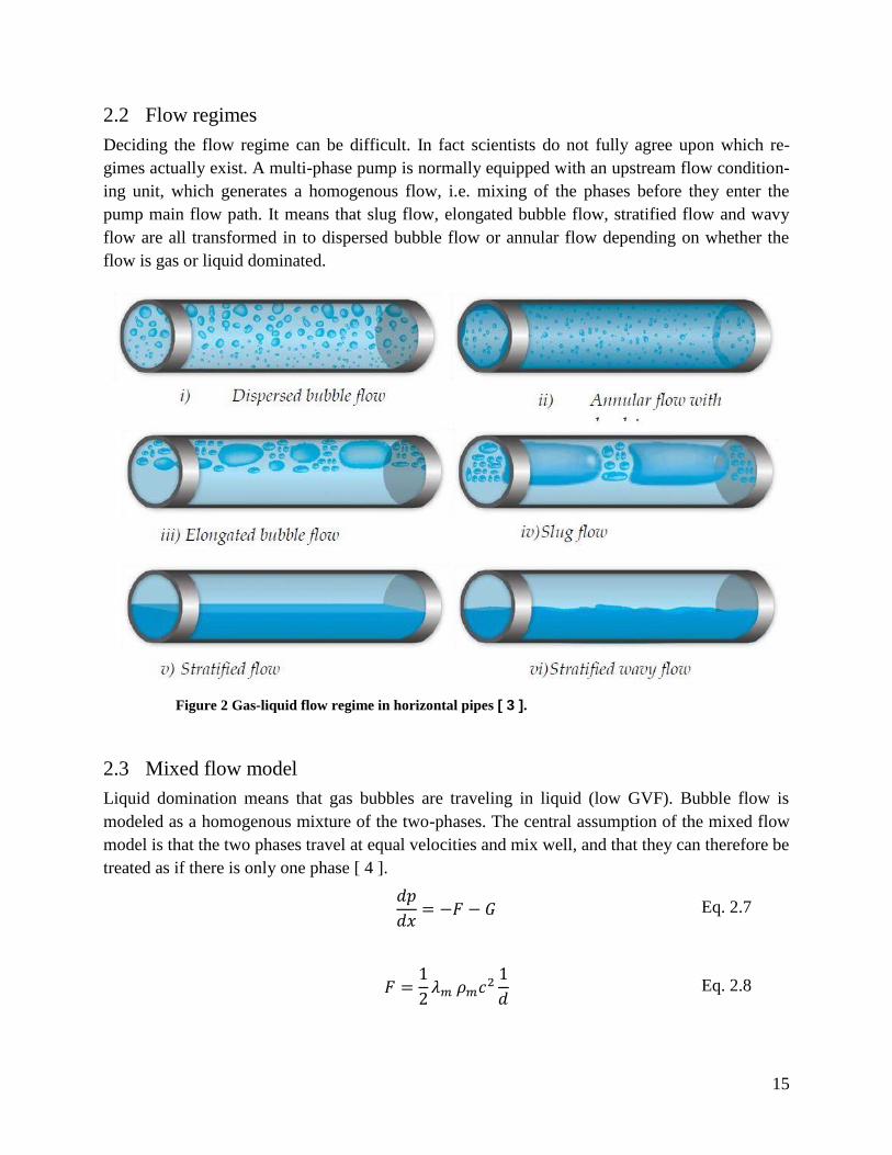
2.2 Flow regimes
Deciding the flow regime can be difficult. In fact scientists do not fully agree upon which re-
gimes actually exist. A multi-phase pump is normally equipped with an upstream flow condition-
ing unit, which generates a homogenous flow, i.e. mixing of the phases before they enter the
pump main flow path. It means that slug flow, elongated bubble flow, stratified flow and wavy
flow are all transformed in to dispersed bubble flow or annular flow depending on whether the
flow is gas or liquid dominated.
Figure 2 Gas-liquid flow regime in horizontal pipes [ 3 ].
2.3 Mixed flow model
Liquid domination means that gas bubbles are traveling in liquid (low GVF). Bubble flow is
modeled as a homogenous mixture of the two-phases. The central assumption of the mixed flow
model is that the two phases travel at equal velocities and mix well, and that they can therefore be
treated as if there is only one phase [ 4 ].
Eq. 2.7
Eq. 2.8

16
Eq. 2.9
Eq. 2.10
Eq. 2.7 represents the momentum equation for pipe flow with constant cross sectional area. The
effect of mixture friction against the pipe wall (F) is given in Eq. 2.8 while gravitational effect on
pressure change (G) is described by Eq. 2.9. Mixed-fluid density is determined by averaging the
densities.
2.4 Two-fluid model
The drag force of a bubble travelling in a liquid is significant compared to its mass, therefore the
bubble quickly adapts to any changes in the liquid velocity. For gas dominated flow however the
drag force of the liquid droplet is small compared to its mass, and homogeneous fluid theory is
therefore not valid. Instead a two-fluid model must be applied [ 4 ].
Eq. 2.11
Eq. 2.12
The two-fluid model separates the gas and the liquid into two different momentum equations.
Because slip between the phases is expected, area fractions are introduced. Eq. 2.11 is the gas
momentum equation while Eq. 2.12 represents the momentum equation for the liquid droplets.
The pressure loss due to drag on the droplets is given by . If a liquid film exists together with
gas and liquid droplets, which is often the case for annular flow, the liquid holdup has to be sepa-
rated into film holdup and droplet holdup. A third momentum equation must also be added to
handle the liquid film.

17
18
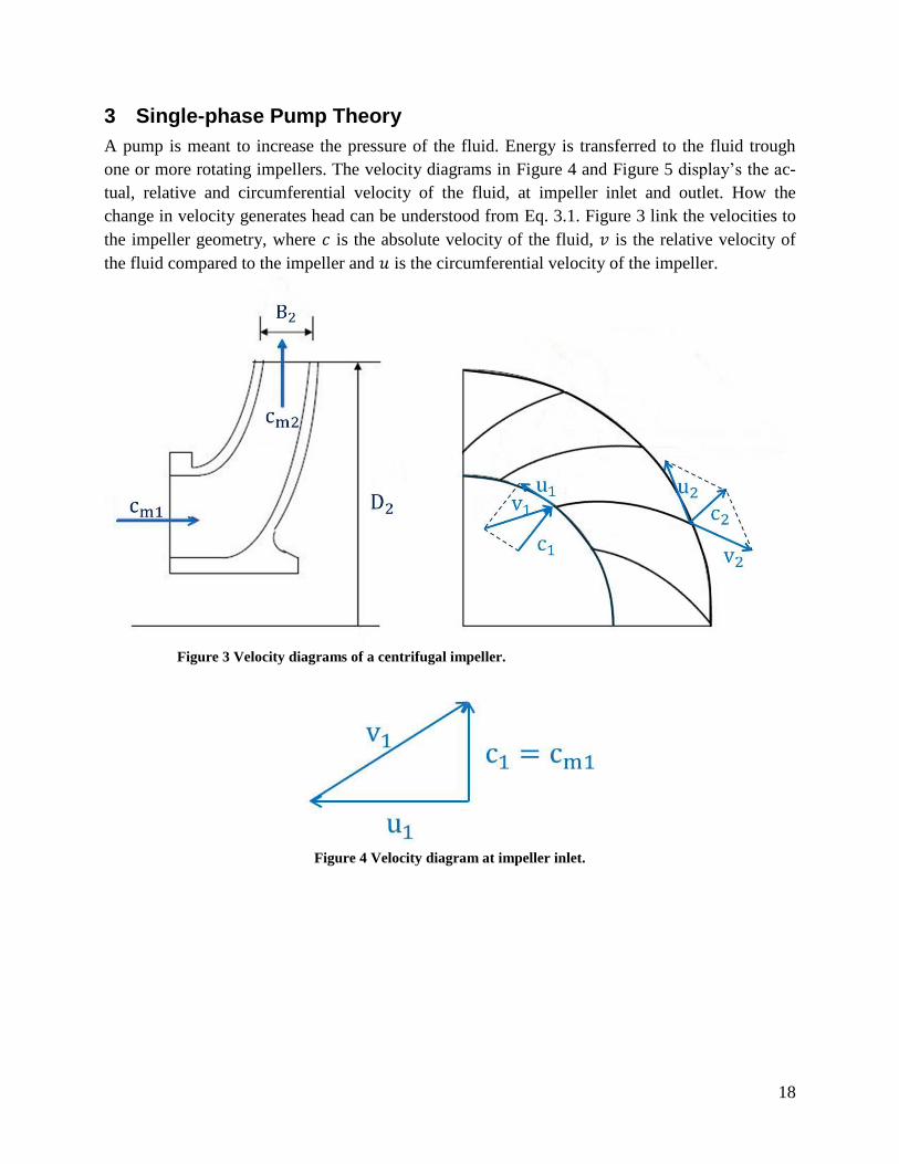
3 Single-phase Pump Theory
A pump is meant to increase the pressure of the fluid. Energy is transferred to the fluid trough
one or more rotating impellers. The velocity diagrams in Figure 4 and Figure 5 display’s the ac-
tual, relative and circumferential velocity of the fluid, at impeller inlet and outlet. How the
change in velocity generates head can be understood from Eq. 3.1. Figure 3 link the velocities to
the impeller geometry, where is the absolute velocity of the fluid, is the relative velocity of
the fluid compared to the impeller and is the circumferential velocity of the impeller.
Figure 3 Velocity diagrams of a centrifugal impeller.
Figure 4 Velocity diagram at impeller inlet.
19
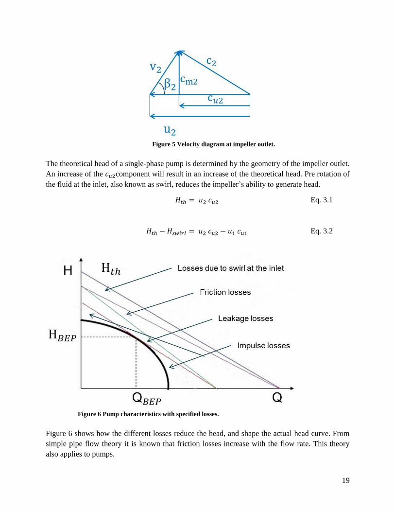
Figure 5 Velocity diagram at impeller outlet.
The theoretical head of a single-phase pump is determined by the geometry of the impeller outlet.
An increase of the component will result in an increase of the theoretical head. Pre rotation of
the fluid at the inlet, also known as swirl, reduces the impeller’s ability to generate head.
Eq. 3.1
Eq. 3.2
Figure 6 Pump characteristics with specified losses.
Figure 6 shows how the different losses reduce the head, and shape the actual head curve. From
simple pipe flow theory it is known that friction losses increase with the flow rate. This theory
also applies to pumps.

20
Leakage flow in a typical centrifugal pump can consist of;
flow from the impeller discharge back to suction trough the wear ring at the front shroud,
flow from impeller suction through the wearing separating the diffuser and the shaft,
flow through an axial thrust force balancing device.
A flow will increase if the differential pressure over its path increases. Leakage losses have the
same effect, and are increasing with increasing head.
Impeller inlet and outlet are designed so that neither flow separation nor recirculation (backward
facing flow) occurs at the best efficiency point [ 2 ]. These types of losses are referred to as im-
pulse losses. When operating outside the design point, impulse losses exist due to miss match
between the flow and the shape of the impeller
An accurate determination of the different losses requires details about geometry and fluid behav-
ior. Such information is not easily obtained. Performance predictions of a single-phase pump are
therefore done based on characteristics from a similar and already tested pump. A set of scaling
rules are used in these calculations. Head, power consumption and flow rate are primarily scaled
according to the affinity laws, in order to fit the correct diameter and rotational speed of the im-
peller. If the amount of stages differs between the predicted and the tested pump, head and power
are also scaled according to the application/model stage count ratio. At last, if the density of the
tested fluid differs from the fluid in the predictions, power consumption is scaled according to the
application/model density ratio [ 2 ].
Application/model stage count ratio:
Eq. 3.3
Eq. 3.4
Application/model density ratio:
Eq. 3.5
3.1 Affinity laws
The affinity laws are derived from a dimensionless analysis and are widely used for scaling per-
formance curves of radial impeller pumps. The analysis is based on geometrical similarity and
constant pump efficiency.
21
Eq. 3.6
Eq. 3.7
Eq. 3.8
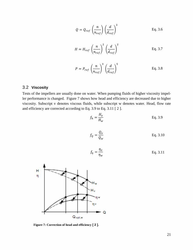
3.2 Viscosity
Tests of the impellers are usually done on water. When pumping fluids of higher viscosity impel-
ler performance is changed. Figure 7 shows how head and efficiency are decreased due to higher
viscosity. Subscript v denotes viscous fluids, while subscript w denotes water. Head, flow rate
and efficiency are corrected according to Eq. 3.9 to Eq. 3.11 [ 2 ].
Eq. 3.9
Eq. 3.10
Eq. 3.11
Figure 7: Correction of head and efficiency [ 2 ].
22
There are many available viscosity correction models, most of them are empirical. The Hydraulic
Institute model is used and accepted by industry worldwide. It has been included as an ISO
standard and is meant to include all centrifugal and vertical pumps, with open or closed impellers,
single or double suction, pumping Newtonian fluids [ 5 ].
Eq. 3.12
Eq. 3.13
The model consists of equations based on a “pump performance Reynolds number”, adjusted for
specific speed (parameter B).
Eq. 3.14
Eq. 3.15
Eq. 3.16
Eq. 3.17
Eq. 3.18
Eq. 3.19
The correction factor for flow and efficiency is calculated from parameter B. The head correction
factor at best efficiency point equals the flow correction factor. Eq. 3.19 then adjusts the head for
different flow rates.

23

24
4 Multi-phase Pump Theory
A significant difference between multi-phase and single-phase performance predictions is that
multi-phase predictions should be done stage by stage. The outlet conditions of the previous stage
acts as inlet conditions to the following stage. This is because important performance parameters
such as density ratio (DR) and GVF are constantly changing throughout the compression.
4.1 Affinity and Similarity laws
In chapter 3.1 the affinity laws were introduced. The affinity laws scale performance of radial
impellers when the outlet diameter or rotational speed is changed. Because radial impellers are
more exposed to formation of gas blockages, semi-axial impellers are preferred when the gas
content is significant. For typical semi-axial impellers, all geometric dimensions have to be
scaled in order to keep similarity, not just the outlet diameter. The similarity laws are therefore
applied instead of the affinity laws.
Similarity laws:
Eq. 4.1
Eq. 4.2
Eq. 4.3
The affinity and similarity laws are commonly used and accepted for centrifugal and semi-axial
impellers. When pumping multi-phase flow these laws show good accuracy for liquid dominated
flow. For gas dominated flow however the scaling laws does not apply [ 6 ].
A way around the limitations of the scaling laws is to avoid applying them directly on multi-
phase flow. Scaling can be done on single-phase test data in order to calculate the single-phase
flow coefficients before multi-phase effects are considered. The effects of operating with gas
dominated flow are later captured by the two-phase multipliers and not the scaling laws.

25
4.2 Two-phase multipliers
Two-phase multipliers are used to predict two-phase performance when single-phase perfor-
mance of liquid is known. The single-phase performance is found according to chapter 3. Gas
entering the pump will cause degradation of the head as well as reduction in power consumption.
Rune Mode Ramberg [ 7 ] states the degradation of the head is related to the amount of gas going
through the pump, the density of the mixture, the density ratio, the inlet pressure, the inlet tem-
perature and the viscosity. He also mentions that pump speed is important. Too high speed will
lead to fluid separation and reduce the performance even more. The two-phase multipliers are
defined in the following way.
Head degradation factor:
Eq. 4.4
Power consumption reduction factor:
Eq. 4.5
From here on the thesis refers to the two-phase multipliers presented in Eq. 4.4 and Eq. 4.5 as
head degradation factor and power consumption reduction factor. A set of two-phase multipliers
generated from experiments are used as input in the performance predictions. Single- and two-
phase flow coefficients form the basis when calculating the head degradation factors. The coeffi-
cients are generated from test results and related to each other by the same volumetric flow rate.
They are found by measuring inlet and outlet conditions as well as impeller tip speed.
Eq. 4.6
In chapter 2 it was shown that liquid dominated flow could be modeled as a homogenous mix-
ture. When it comes to multi-phase head calculations the two-fluid model is applied in order to
treat the gas and the liquid differently.
Eq. 4.7
Eq. 4.8
As well as for calculating the head degradation factor from test results, Eq. 4.7 is used to predict
two-phase head when the head degradation factor is known. Stage outlet pressure can be calculat-
ed from Eq. 4.7 once the two-phase head is determined. Note that Eq. 4.7 applies an isothermal
compression model for the gas part of the equation. Alternatives to this approach will be present-
ed later.

26
The power consumption reduction factors can be determined by relating power consumptions
from single- and two-phase test data. The test data share the same flow rate and rotational speed.
Gülich [ 2 ] states that if a pump is operated with a given two-phase mixture at specific flow rate
ratio with different speeds, the velocity triangles remain similar. Therefore two-phase multi-
pliers can be used independently of impeller tip speed and consequently independently of diame-
ter and rotational speed of the pump.
4.2.1 Analytical approach
Ramberg developed a head degradation factor, which can be calculated analytically from varia-
bles that are easily obtained under actual operating conditions. He evaluated the influence of
GVF, density ratio, mixture density, inlet pressure, inlet temperature, pump speed and came up
with the model given in Eq. 4.9.
Eq. 4.9
Eq. 4.10
By rearranging Eq. 4.9 we can see in Eq. 4.10 that Ramberg’s head degradation factor only de-
pends on the GVF and the density ratio. He has tested and validated the model against actual
pump performance at the oil and gas field Gullfaks.
4.2.2 MIT-model
The MIT-model is presented in the master thesis of J. E. Korenchan [ 11 ]. This model is a result
of nuclear research, and an attempt to understand how pumps are affected by air or steam. Instead
of looking at degradation of the head, MIT focused on how the head loss was increasing with
increasing GVF. Korenchan states that by normalizing two-phase head loss compared to single-
phase head loss instead of normalizing two-phase head compared with single-phase head we can
diminish the dependence of pump geometry. Eq. 4.11 shows how the head-loss ratio where
defined.
Eq. 4.11
Eq. 4.12

27
A lot of challenges are involved when applying the MIT-model, one of them is determination of
the slip factor μ. Note that μ does not represent the slip between the phases, but the slip angle at
the trailing edge of the impeller. The slip factor is needed to calculate the outlet flow angle
which affects the calculation of the head coefficient. An empirical method by Noorbakhsh [ 13 ]
was suggested to determine the slip factor. Another challenge is to determine the slip ratio S (slip
between the phases) which is needed in order to calculate the two-phase flow function .
The idea of looking at head loss increase instead of head decrease is interesting, and might result
in more accurate predictions. The uncertainty however, related to estimating the outlet flow angle
is great. The empirical method of Noorbakhsh could be applied, but first it should be validated
against CFD-simulations of the actual impeller.
4.3 Gas compression
As seen in subchapter 4.2, isothermal compression was applied in order to calculate the head deg-
radation factor. This chapter will explain the consequences of assuming isothermal compression,
and explain why the polytrophic compression is more accurate, especially in the high GVF re-
gion. It will also highlight additional input data required for an implementation a polytrophic
compression model.
4.3.1 Isothermal compression
A process that occurs at constant temperature is called an isothermal process. The liquid phase in
a two-phase flow holds a significant larger heat capacity per unit volume compared to the gas
phase. A high GVF value is needed to get a noticeable heat increase. A normal assumption is
therefore that the gas goes through an isothermal compression process.
Head:
Eq. 4.13
Assuming ideal gas:
Eq. 4.14
Constant temperature:
Eq. 4.15
Rearranging Eq. 4.14 and including constant temperature:
Eq. 4.16
Applying the isothermal relation (Eq. 4.16) in Eq. 4.15 to get the isothermal head:

28
Eq. 4.17
The isothermal compression is a normal simplification applied by the industry. Heat generated
from compression of the gas is neglected and the temperature is assumed constant from suction to
discharge.
4.3.2 Polytrophic compression
A possible improvement of multi-phase pump performance predictions would be to replace iso-
thermal calculations with a polytrophic approach. It will influence the calculation of head degra-
dation factor, stage outlet pressure and overall efficiency of the pump. As no heat is neglected,
the polytrophic compression model is believed to improve the calculations. Before showing how
it can be implemented in multi-phase predictions, we shall take a short review of the polytrophic
gas compression process.
Polytrophic relation:
Eq. 4.18
Rearranging:
Eq. 4.19
Inserting the polytrophic relation in Eq. 4.13 to get the polytrophic head:
Eq. 4.20
Schultz
The polytrophic head given in Eq. 4.20 is not correct because the change in polytrophic exponent
along the compression path is neglected. Schultz [ 14 ] introduced the volume corrected poly-
trophic exponent and the compressibility functions X and Y.
Eq. 4.21
Eq. 4.22
29
Eq. 4.23
The change in along the compression path is considered to be small. Schultz defined it as con-
stant. He introduced the compression path correction factor to correct for the small variations
in .
Eq. 4.24
Where:
Eq. 4.25
Schultz definition of the polytrophic head is finally given by:
Eq. 4.26
Applying Schultz`s polytrophic head into Eq. 4.7 would be a improvement compared to the iso-
thermal predictions, but it requires more thermodynamic data on the gas phase. A possibility
could be to involve a process simulation tool such as HYSYS in the predictions.
The following work will continue by showing how the polytrophic head from Eq. 4.20 can be
used to predict performance of a multi-phase pump. By applying Eq. 4.20 instead of Eq. 4.26 no
process simulation program is necessary.
First we establish head degradation factor data from single and two-phase tests. The actual two-
phase head is found from Eq. 4.27. Then polytrophic efficiency data is calculated. It can be re-
trieved from test results by solving the first two sections of Eq. 4.28 iteratively. Note that the re-
lation / = / used for compressors, is valid only for pure gas and
cannot be used to calculate polytrophic efficiency from two-phase test data [ 14 ].
Eq. 4.27
Eq. 4.28
.
30
Eq. 4.29
Where:
Eq. 4.30
And
Eq. 4.31
Eq. 4.32
The established test data can now be used to predict outlet pressure from last two sections of Eq.
4.28, and outlet temperature from Eq. 4.32.
4.4 Viscosity
Discovery and development of new oilfields causes the industry to demand pumps that can han-
dle fluids of higher viscosities. From chapter 3.2 we know that viscosity correction of single-
phase pump performance is commonly used and accepted. For multi-phase flow, viscosity impact
on fluid behavior becomes more complex. It is difficult to establish which phase is in contact
with the surrounding geometry, how the viscosities affect the flow pattern and how the two phas-
es interact with each other.
When pumping multi-phase flow the drag of the bubbles rise with the viscosity of the liquid
phase. An increase in the viscosity is expected to work against phase separation. Gulich [ 2 ]
found that by increasing viscosity from 10 and 18 /s performance actually improved at flow
rates above best efficiency flow rate. Generally, increased viscosity reduces performance of sin-
gle-phase pumps.
Viscous effects can be predicted trough a multi-phase fluid viscosity. This viscosity is a combina-
tion of the fluid viscosity and the liquid viscosity. Rune Mode Ramberg [ 7 ] stated that this kind
of approach causes a mal-interpretation of the viscous effects. Instead he introduced the apparent
liquid viscosity correlations, which are based on Reynolds number correction’s to turbulent flow
in pipes. The semi-empirical model corrects for efficiency, head and flow rate.
31
Eq. 4.33
Eq. 4.34
Eq. 4.35
The idea is basically to correct for viscous effects before applying the two-phase multiplier. As a
result, we only have to deal with viscosity of one phase. Another favourable aspect is that we are
more likely to utilize the correct two-phase multiplier when performance already is corrected for
viscosity.
Ramberg has verified the correlations against both single and multi-phase test results. He found
them to give reasonable results for viscosities less than 90 cSt. For higher viscosities he found
degradation of head and flow rate to be at some extent overestimated.
4.5 Phase transition
When a multi-phase mixture is compressed, temperature and pressure increases. A change in gas
mass fraction from stage inlet to outlet can occur as a result of some gas or liquid changing phase.
Phase transitions are often neglected and the gas mass fraction is assumed constant from suction
to discharge.
Eq. 4.36
If phase transition is to be included in predictions it can either be added directly in to the head
equation as in the last section of Eq. 4.36, or the gas mass fractions can be corrected to fit the end
state after stage outlet temperature and pressure is predicted. In both ways a process simulation
tool such as HYSYS is needed to provide the thermodynamic data.
32
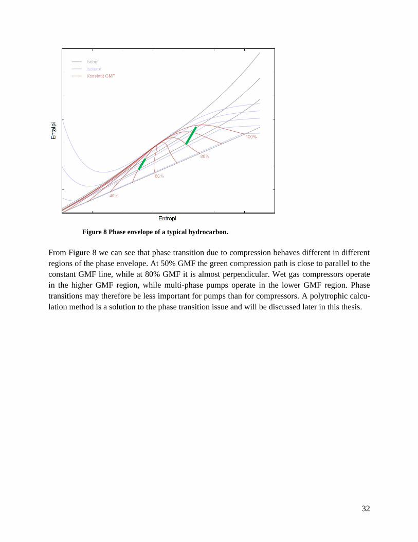
Figure 8 Phase envelope of a typical hydrocarbon.
From Figure 8 we can see that phase transition due to compression behaves different in different
regions of the phase envelope. At 50% GMF the green compression path is close to parallel to the
constant GMF line, while at 80% GMF it is almost perpendicular. Wet gas compressors operate
in the higher GMF region, while multi-phase pumps operate in the lower GMF region. Phase
transitions may therefore be less important for pumps than for compressors. A polytrophic calcu-
lation method is a solution to the phase transition issue and will be discussed later in this thesis.

33
34
5 Temperature measurements
As seen in Chapter 4.3, the polytrophic compression model could be an improvement of the per-
formance calculation routine. The polytrophic compression model requires test data containing
temperature measurements. This chapter will highlight the importance of accurate temperature
measurements and introduce different type of temperature sensors.
5.1 Accuracy
Discharge temperature measurements are usually not included in single-phase pump performance
tests, as the compression is assumed isothermal. On the compressor side the ISO standard for
performance tests states that a inaccuracy should be less than 1 K when it comes to temperature
measurements [ 19 ]. For multi-phase flow an accuracy of 1 K is not accurate enough, as the tem-
perature difference between impeller inlet and outlet is often just a couple degrees C. Two sensi-
tivity analyses presented in the project thesis “MultiBooster Performance” [ 17 ], written by the
author of this Master thesis will now be revisited.
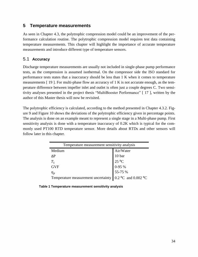
The polytrophic efficiency is calculated, according to the method presented in Chapter 4.3.2. Fig-
ure 9 and Figure 10 shows the deviations of the polytrophic efficiency given in percentage points.
The analysis is done on an example meant to represent a single stage in a Multi-phase pump. First
sensitivity analysis is done with a temperature inaccuracy of 0.2K which is typical for the com-
monly used PT100 RTD temperature sensor. More details about RTDs and other sensors will
follow later in this chapter.
Temperature measurement sensitivity analysis
Medium Air/Water
∆P 10 bar
25 ⁰C
GVF 0-95 %
55-75 %
Temperature measurement uncertainty 0.2 ⁰C and 0.002 ⁰C
Table 1 Temperature measurement sensitivity analysis
35
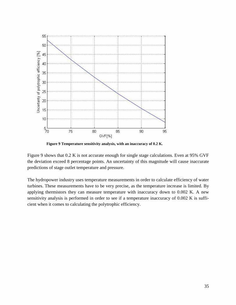
Figure 9 Temperature sensitivity analysis, with an inaccuracy of 0.2 K.
Figure 9 shows that 0.2 K is not accurate enough for single stage calculations. Even at 95% GVF
the deviation exceed 8 percentage points. An uncertainty of this magnitude will cause inaccurate
predictions of stage outlet temperature and pressure.
The hydropower industry uses temperature measurements in order to calculate efficiency of water
turbines. These measurements have to be very precise, as the temperature increase is limited. By
applying thermistors they can measure temperature with inaccuracy down to 0.002 K. A new
sensitivity analysis is performed in order to see if a temperature inaccuracy of 0.002 K is suffi-
cient when it comes to calculating the polytrophic efficiency.

36
Figure 10 Temperature sensitivity analysis, with an inaccuracy of 0.002 K.
Figure 10 shows that calculations of the polytrophic efficiency are significantly improved when
the inaccuracy of the temperature measurements is reduced to 0.002 K. At GVFs above 60% it is
less than 0.75 percentage points, which must be found acceptable.
5.2 Sensor technologies
Accurate temperature measurements are crucial when it comes to evaluating performance of mul-
ti-phase pumps. Temperature cannot be measured directly, instead we measure quantities that are
temperature dependant. This chapter will describe and evaluate different types of temperature
sensors that are relevant for measuring multi-phase flow.
5.2.1 Thermocouples
Thermocouples are the most versatile thermometer. They utilize the fact that when a homogenous
conductor is heated locally it generates a voltage potential. The hot part becomes positively
charged compared to the cold part, and the voltage measured between them is proportional to the
temperature difference and the Seebeck coefficient of the conductor.
Eq. 5.1
37
When two conductors made of different materials are connected together and exposed to different
temperatures, a voltage potential between the two junctions can be measured. The measured volt-
age depends on the temperature difference and the Seebeck coefficients of the two conductors.
Eq. 5.1 shows the relation between the measured voltage , the Seebeck coefficients and the
temperature difference.
The relation between the Seebeck coefficients and the temperature is none linear. In order to gen-
erate accurate measurements the temperature of the reference junction could be held constant.
Another more commonly used method is to utilize hardware or software based cold junction
compensation. Cold junction compensation reduces the generated voltage to a voltage that corre-
sponds with the reference temperature.
Thermocouples can measure over a large temperature span, and if the hot junction is sufficiently
small they can respond quickly to changes in temperature. The main limitation is their accuracy.
5.2.2 Resistance temperature detectors (RTD)
Resistance temperature detectors (RTDs) are more accurate thermometers. They measure the
resistance of a conductor. The resistance of a conductor depends on temperature and on the mate-
rial. The relation between temperature and resistance can be expressed by Eq. 5.2. The number of
joints required in the equation, depends on the wanted accuracy and temperature span.
Eq. 5.2
Resistance is measured by subjecting the conductor to a current. As the current heats the conduc-
tor, the temperature rises above the surrounding temperature, and the measurements becomes
inaccurate. To reduce this effect, a larger conducting element could be chosen. Although this re-
duces the temperature gradient, it generates another limitation. The extra mass increases the re-
sponse time of the detector, which is an important parameter when it comes to measuring multi-
phase flow. The final selection of conductor will have to be a trade-off between response time
and accuracy. Either way it is important to keep the measuring current low.
Typically RTDs are made from Platinum or Nickel. Platinum has a wide temperature span and
good linearity. Nickel is the cheapest option, but its temperature span is limited.
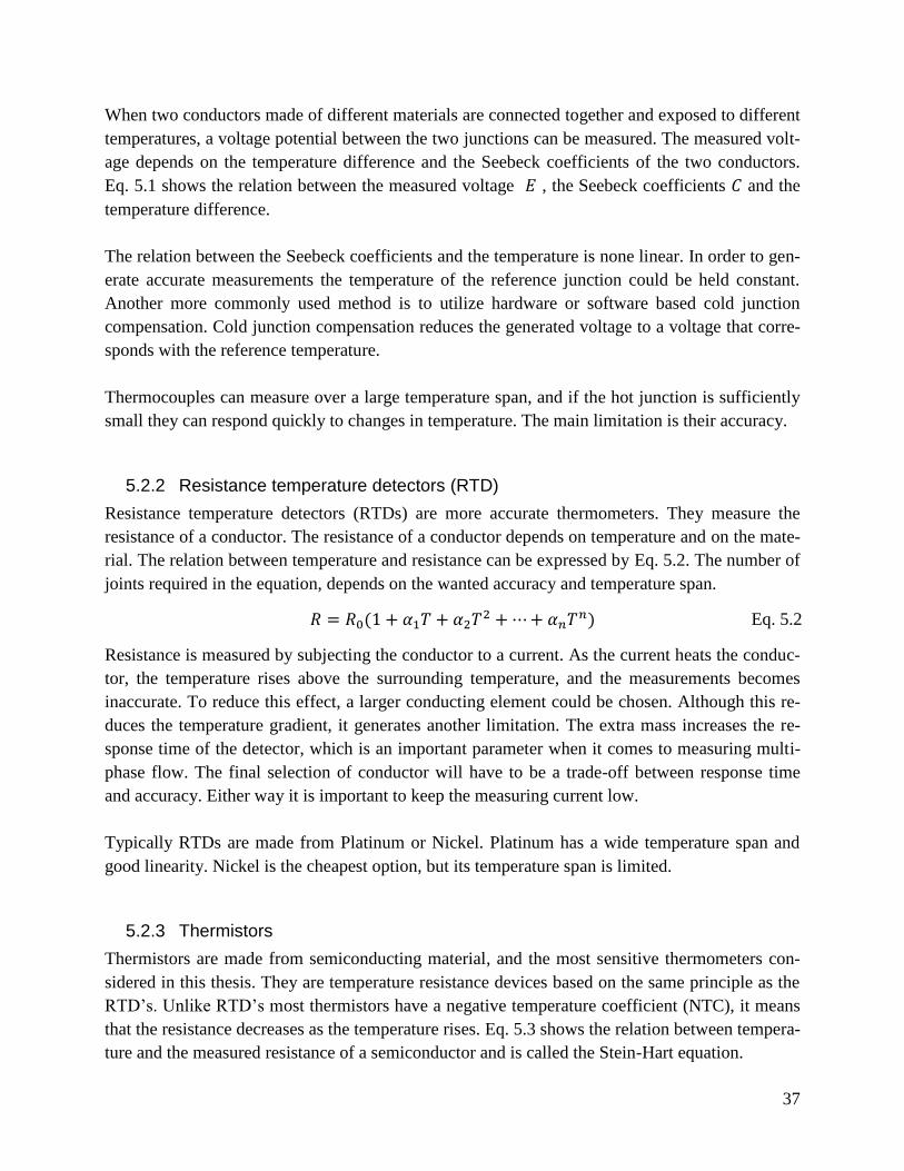
5.2.3 Thermistors
Thermistors are made from semiconducting material, and the most sensitive thermometers con-
sidered in this thesis. They are temperature resistance devices based on the same principle as the
RTD’s. Unlike RTD’s most thermistors have a negative temperature coefficient (NTC), it means
that the resistance decreases as the temperature rises. Eq. 5.3 shows the relation between tempera-
ture and the measured resistance of a semiconductor and is called the Stein-Hart equation.
38
Eq. 5.3
Thermistors are usually made from oxides, but silicates and sulfides are also used.
Figure 11 Comparison of RTDs, NTC thermistors and Thermo couples.
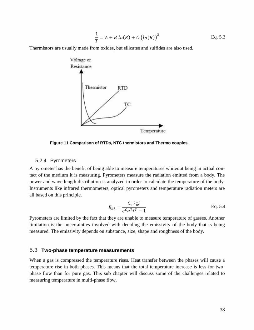
5.2.4 Pyrometers
A pyrometer has the benefit of being able to measure temperatures whiteout being in actual con-
tact of the medium it is measuring. Pyrometers measure the radiation emitted from a body. The
power and wave length distribution is analyzed in order to calculate the temperature of the body.
Instruments like infrared thermometers, optical pyrometers and temperature radiation meters are
all based on this principle.
Eq. 5.4
Pyrometers are limited by the fact that they are unable to measure temperature of gasses. Another
limitation is the uncertainties involved with deciding the emissivity of the body that is being
measured. The emissivity depends on substance, size, shape and roughness of the body.
5.3 Two-phase temperature measurements
When a gas is compressed the temperature rises. Heat transfer between the phases will cause a
temperature rise in both phases. This means that the total temperature increase is less for two-
phase flow than for pure gas. This sub chapter will discuss some of the challenges related to
measuring temperature in multi-phase flow.

39
First of all GVF affects the temperature increase. For single-phase pumps pressure increase is the
main concern. On the compressor side the temperature increase is highly significant. For multi-
phase pumps operating on gas/liquid mixtures, temperature measurements need to be very accu-
rate, as the temperature increase is limited by the liquid content.
There is some uncertainty related to kinetics involved with heat exchange between the gas and
liquid phases. If the gas is heated rapidly, a temperature difference might develop between the
phases. If the phases are not in thermal equilibrium, the local phase temperatures need to be
measured separately. It is also important to know which of the two phases that is actually being
measured.
For liquid dominated flow, HZDR-innovation provides a thermo-needle-probe system which is
designed to do local phase temperature measurements for multi-phase flow [ 27 ]. The probe
combines temperature measurements and conductivity measurements. The temperature sensor
consists of a small thermocouple which responds fast enough to measure temperatures of passing
gas bobbles. The conductivity tells us which phase the needle is subjected to. If the conductivity
is zero for a longer time than the response time of the thermocouple, the probe is measuring the
gas temperature. Figure 12 shows the measured temperature and conductivity of a passing bob-
ble.
Figure 12 Temperature and conductivity measurement of a passing bobble [ 27 ].

40
For gas dominated flow the combined temperature conductivity sensor only work as a standard
temperature sensor. The conductivity which is measured between the probe tip and ground poten-
tial will be zero both when the probe tip is subjected to gas and when it is covered by a liquid
droplet. Ground potential is often the pipe wall, and unless there exists continues liquid between
it and the probe tip, no conductivity will be measured.
Due to the nature of gas dominated flow the heat exchange between the phases is slower than for
liquid dominated flow. The heat capacity of the liquid droplets is high and the surface area is
small, therefore it is more likely that a temperature difference will occur in gas dominated flow.
Another problem related to temperature measurements in gas dominated flow is the formation of
liquid films on all surfaces including the sensors. If the probes are covered with liquid, they will
simply measure the liquid temperature, and it will be impossible to decide the actual enthalpy of
the mixture.
At last but not least it is worth mentioning that the sensitivity analysis presented early in this
chapter was based upon the assumption that thermal equilibrium existed at the measuring point.
When measuring local phase temperature in none equilibrium mixtures, the gas temperature
measurements does not have to be as accurate as the liquid temperature measurements. It is be-
cause a given change in gas temperature will have less effect on the enthalpy than the same
change in liquid temperature.

41
42
6 Laboratory rig
The goal of this chapter is to plan a test rig that can validate different temperature sensors ability
to give accurate measurements of multi-phase flow. Main focus will be appointed to conditions
where thermal equilibrium is not met.
A polytrophic compression model can improve performance predictions of multi-phase pumps.
Unlike the isothermal model they require temperature measurements. These measurements will
have to be taken stage-by-stage, in locations where the phases might not be in thermal equilibri-
um. Temperature measurements will have to be measured locally in each phase. Although the
industry seems to assume thermal equilibrium, no documentation has so far been found on this
topic.
For multi-phase pumps, the temperature increase is limited, especially when it comes to stage-by-
stage and low GVF calculations. As explained earlier, the limited temperature is caused by the
high heat capacity per unit volume of the liquid compared to the heat capacity per unit volume of
the gas. Temperature measurements will therefore have to be highly accurate. The test rig shall
generate conditions where the two-phase mixture is not in thermal equilibrium. And the tempera-
ture sensors will be evaluated by their ability to do accurate local temperature measurements.
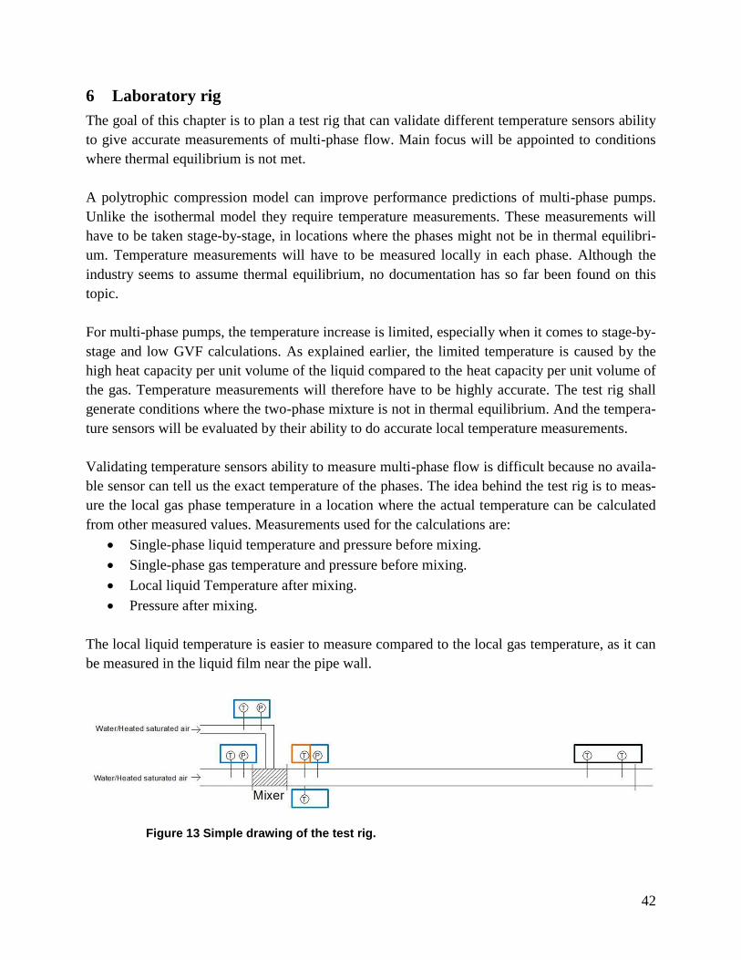
Validating temperature sensors ability to measure multi-phase flow is difficult because no availa-
ble sensor can tell us the exact temperature of the phases. The idea behind the test rig is to meas-
ure the local gas phase temperature in a location where the actual temperature can be calculated
from other measured values. Measurements used for the calculations are:
Single-phase liquid temperature and pressure before mixing.
Single-phase gas temperature and pressure before mixing.
Local liquid Temperature after mixing.
Pressure after mixing.
The local liquid temperature is easier to measure compared to the local gas temperature, as it can
be measured in the liquid film near the pipe wall.
Figure 13 Simple drawing of the test rig.
43
The orange square in Figure 13 is the local gas phase measurement. The measured gas tempera-
ture will be validated against the calculated gas temperature. Blue squares indicate inputs to the
calculations. The black square downstream indicates two temperature measurements that will
measure the equilibrium temperature.
Test procedure, conditions, equipment and different challenges involved with planning the test
rig will be presented in the following subchapters. Data sheets related to the suggested compo-
nents can be found in Appendix B.
Most of the simulations in this chapter are done in HYSYS. HYSYS is a process modeling sys-
tem that allows us to choose different equations of state, fluid compositions and process compo-
nents. Hunseid [ 21 ] found GERG to be the best equation of state for predicting outlet conditions
of a wet gas compressor. GERG is not implemented in the student version of HYSYS, Peng Rob-
inson is therefore used in the following simulations. In the work of Hunseid, Peng Robinson was
found to be the second best equation of state for predicting outlet conditions.
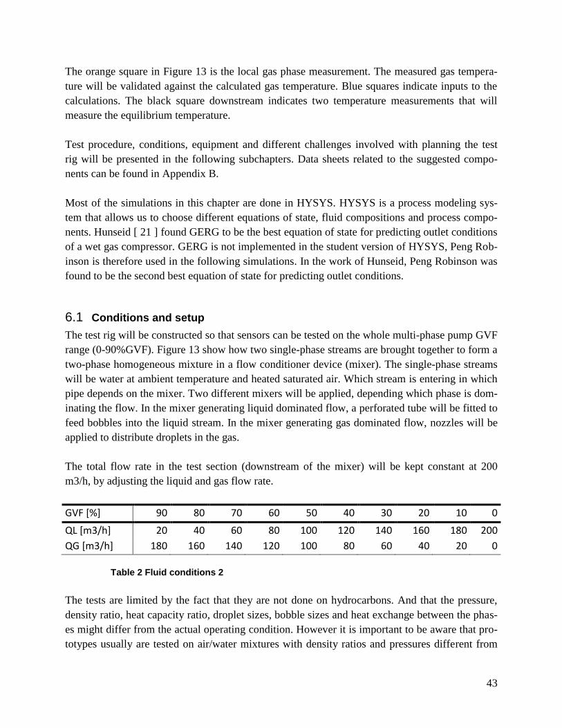
6.1 Conditions and setup
The test rig will be constructed so that sensors can be tested on the whole multi-phase pump GVF
range (0-90%GVF). Figure 13 show how two single-phase streams are brought together to form a
two-phase homogeneous mixture in a flow conditioner device (mixer). The single-phase streams
will be water at ambient temperature and heated saturated air. Which stream is entering in which
pipe depends on the mixer. Two different mixers will be applied, depending which phase is dom-
inating the flow. In the mixer generating liquid dominated flow, a perforated tube will be fitted to
feed bobbles into the liquid stream. In the mixer generating gas dominated flow, nozzles will be
applied to distribute droplets in the gas.
The total flow rate in the test section (downstream of the mixer) will be kept constant at 200
m3/h, by adjusting the liquid and gas flow rate.
GVF [%] 90 80 70 60 50 40 30 20 10 0
QL [m3/h] 20 40 60 80 100 120 140 160 180 200
QG [m3/h] 180 160 140 120 100 80 60 40 20 0
Table 2 Fluid conditions 2
The tests are limited by the fact that they are not done on hydrocarbons. And that the pressure,
density ratio, heat capacity ratio, droplet sizes, bobble sizes and heat exchange between the phas-
es might differ from the actual operating condition. However it is important to be aware that pro-
totypes usually are tested on air/water mixtures with density ratios and pressures different from

44
actual operating conditions, and that the performance of the pump often is predicted from
air/water test results. Being able to do local phase temperature measurements of air/water mix-
tures is therefore important in a research and developing point of view as well as a step into doing
local phase measurements in the field.
Figure 14 Heater and saturator simulations.
In order to generate a temperature difference between the phases, the gas enters the mixer fully
saturated and heated to 60 degree C. Liquid enters with an ambient temperature. The reason for
saturating the air will be explained later.
Figure 14 shows how the heater and saturator is simulated in HYSYS. The heater must be able to
deliver at least 10.58 kW of heat, to maintain a gas temperature of 60 degree C at a GVF of 90%.
The saturator must be able to feed at least 10.8 kg/h of water to saturate gas.
6.2 Engineering
This subchapter will go through the challenges and solutions related to the engineering of the test
rig, by taking a closer look at the following subjects.
Temperature measurements
Test section

45
Gas phase humidity
Gas volume fraction
Mixers
6.2.1 Temperature measurements
When it comes to choosing temperature sensors, it is all about deciding what you need the meas-
urements fore. As seen in chapter 5 thermistors provide the most accurate measurements, but do
not respond quickly to changes in temperature. They are also limited to a relatively narrow tem-
perature span. RTDs can also be quite accurate but have the same limitations when it comes to
response time. They are preferred by the industry in stationary flow, and can be useful in thermal
equilibrium conditions when accuracy is important.
RTDs and thermistors can also be used to decide whether or not the phases are in thermal equilib-
rium. Framo Engineering used this approach when they tested their wet gas compressor. Four
temperature measurements where done downstream of the compressor discharge. The distances
between the probes were 2 meters. The idea was that Thermal equilibrium was reached when two
or more probes showed the same value. They experienced that thermal equilibrium was reached
already at the discharge, as all four sensors showed the same value within the given uncertainty
of the probes. Note that the tests were done at 95% GVF and above.
In conditions where thermal equilibrium is absent, temperature sensors will be exposed to rapid
changes in temperature, as bobbles or droplets hit the probe tip. There are two obvious ways of
measuring local phase temperature:
Applying a sensor which responds quick enough, to measure the temperature of a passing
bobble or a droplet.
Make sure the sensor is only subjected to one of the phases.
The thermo needle probe system delivered by HZDR utilizes the first measurement principle.
They can do local temperature measurements, and have been tested on liquid dominated flow
with a velocity up to 20m/s. They consist of fast responding small thermocouple junctions. The
probes can also do conductivity measurements. From here on the combined temperature and con-
ductivity probes will be referred to as CTC-probes. Contact has been established, and an official
offer on a 5 customized sensors including cables and software has been received from HZDR.
The offer can be found in Appendix A.
The alternative measurement principle suggests that a more accurate, but slower sensor is sub-
jected to only one of the two phases. Two different approaches subjecting a PT100 sensor to only
the gas phase will be presented in the next subchapter. Also the liquid phase temperature will be
measured using this principle, by positioning a sensor in the liquid film at the bottom of the pipe.

46
Table 3 shows some data on the sensors chosen for this assignment. More can be found in the
data sheets in Appendix B. Details concerning the mounting of the sensors will follow in the next
subchapter.
Name: Type: Accuracy: Response time
CTC Thermocouple 0.7 20 ms
PT100 RTD 0.164 200 ms
SBE38 Thermistor 0.001 500 ms
Table 3 Temperature sensor data
The total enthalpy of the two-phase mixture is highly sensitive to the liquid temperature and not
so sensitive to the gas temperature. This means that for HYSYS to calculate the gas temperature
from the liquid temperature, it needs the liquid temperature measurements to be very accurate.
GVF [%] ∆ ∆
89.58 20.13 39.94 0.001 0.06
Table 4 Sensitivity of liquid temperature measurements on gas temperature calcula-
tions.
A sensitivity analysis displayed in Table 4, shows how an uncertainty in the liquid temperature
measurements affects the uncertainty of the calculated gas temperature. Under the given condi-
tions, an uncertainty of 0.001 in the measured liquid temperature generates an uncertainty in
the calculated gas temperature of 0.06 . From table 3 we read that the SBE38 thermistor will
be accurate enough to measure the liquid temperature, when the goal is to validate gas tempera-
ture measurements taken with the CTC and the RTD100.
6.2.2 Test section
The test section is defined as the pipe work downstream of the mixer. A pressure sensor and two
temperature sensors measuring the gas and liquid phase temperatures are positioned right after
the mixer. Two temperature sensors are also positioned further downstream. Their job is to cap-
ture the equilibrium temperature.
In order to determine the flow regime and view how the sensors are affected by the stream, the
flow will be monitored visually through Plexiglas pipes. The chosen Plexiglas pipes are casted,
have a wall thickness of 10 mm, can withstand a service temperatures of up to 80 and pressures
well above test conditions. More detailed information can be found in the Plexiglas data sheet in
Appendix B.
47
The flow regime in the test section should be as close to the actual discharge conditions of a mul-
ti-phase pump as possible. A pipe diameter of 100 mm combined with a volumetric flow rate of
200 m3/h, generates a fluid velocity of approximately 7m/s, which is a velocity that could also be
found in an actual application. Table 5 shows data related to the flow conditions.
Q [m3/h] r [m] A [m2] v [m/s]
200 0.05 0.00785 7.08
Table 5 Fluid conditions
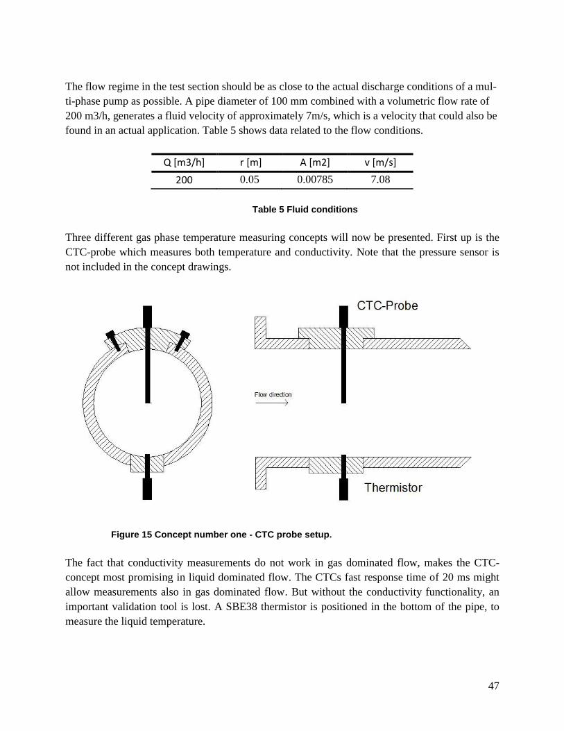
Three different gas phase temperature measuring concepts will now be presented. First up is the
CTC-probe which measures both temperature and conductivity. Note that the pressure sensor is
not included in the concept drawings.
Figure 15 Concept number one - CTC probe setup.
The fact that conductivity measurements do not work in gas dominated flow, makes the CTC-
concept most promising in liquid dominated flow. The CTCs fast response time of 20 ms might
allow measurements also in gas dominated flow. But without the conductivity functionality, an
important validation tool is lost. A SBE38 thermistor is positioned in the bottom of the pipe, to
measure the liquid temperature.

48
Figure 16 Concept number two - PT100 RTD shield setup.
Concept number two is in the first place intended for gas dominated flow. It utilizes a RTD probe
protected by a shield. The idea is that the liquid will be guided around the probe. And as the
probe is not in contact with the shield it will not be affected by the cooling of the liquid. The
drawback of this concept is that gas behind the shield might not be replaced fast enough. If so,
the gas will be cooled by the liquid hitting the shield, which will affect the measurements. As for
the CTC-concept this concept also uses a thermistor to measure the liquid temperature in the bot-
tom of the pipe. The circle to the right in Figure 16 shows how the probe is hidden behind the
shield.

49
Figure 17 Concept number three - PT100 Gas suction setup.
Concept number three is a further development of concept two. It is also intended for gas domi-
nated flow. The idea is to shield the probe from the liquid and at same time replace the gas sur-
rounding the probe. This way temperature will not be affected by the cold shield. Some gas will
be sucked out through the pipe shielding the sensor. It is important that the suction is slow, so
that it doesn`t bring with it any liquid. The drawback with this solution is that it will affect the
equilibrium condition measured by the downstream temperature sensors, as some of the gas is
extracted from the stream. Also this concept utilizes a thermistor positioned in the bottom of the
pipe to measure the liquid temperature. Se Figure 17 for illustration.
Two types of connection points will be used to mount sensors to the Plexiglas pipe, one for the
gas phase temperature measurements and one for all the other sensors. The first type is designed
so that the different gas temperature concepts can be mounted and remounted in different axial
locations of the test section. Why it is so important to be able to move the sensors will be ex-
plained later. The second type will be fabricated from Plexiglas rods and welded onto drilled
holes in the Plexiglas pipe. For illustration, see how the sensors are connected in Figure 17.
Thermal equilibrium will be absent at the moment of mixing, and the goal is to do local tempera-
ture measurements of both phases before equilibrium is reached. No documentation on the heat
transfer between the phases has been found. Focus on multi-phase heat transfer seems to have
been on calculating the heat transfer between the mixture and the surroundings, and not the heat
transfer between the phases. It is therefore difficult to estimate how far the liquid needs to travel
down the pipe in order to reach thermal equilibrium. The length of the test section will have to be
decided by a calculated guess. The suggestion is at least 3m. During tests the equilibrium temper-

50
ature can be found by slowly mowing the two SBE 38 sensors, positioned with some axial dis-
tance, further downstream. The thermal equilibrium is reached at the first sensor when both of
them measure the same value.
The downstream SBE38 sensors will be used to confirm or disprove the measurements in cases
where the local phase temperature sensors do not find a temperature difference between the phas-
es. If all temperature sensors in the test section measures the same temperature, it means that
thermal equilibrium is met already upstream of the local temperature measurements. In that case,
if possible, the local temperature measurements should be moved closer to the mixer.
Uncertainty related to the humidity of the gas, generates a lower boundary on how close to the
mixer the gas measurement can be done. This limitation will be further explained in the next
chapter. Because the position of the sensors is crucial, and that the best position will change with
the conditions, the pipe section will be fitted with as many connection points as possible.
Summary of the needs for measuring instruments in the test section:
One of the concepts above (CTC or RTD) measuring the local gas phase temperature in
the centre of the flow right after mixing.
One SBE38 sensor measuring the liquid temperature at the bottom of the pipe right after
mixing.
Two SBE38 sensors measuring the Temperature of the mixture when thermal equilibrium
is reached in a downstream section of the pipe.
One pressure sensor positioned as close to the local gas phase measurement as possible.
6.2.3 Gas phase humidity
When non saturated air is mixed with water it starts a saturation process. This process requires
heat and causes the temperature of the mixture to drop. It will continue until the air is fully satu-
rated. An example has been run in HYSYS to demonstrate how the saturation affects the tem-
perature, when single-phase liquid and gas with the same temperature is mixed.
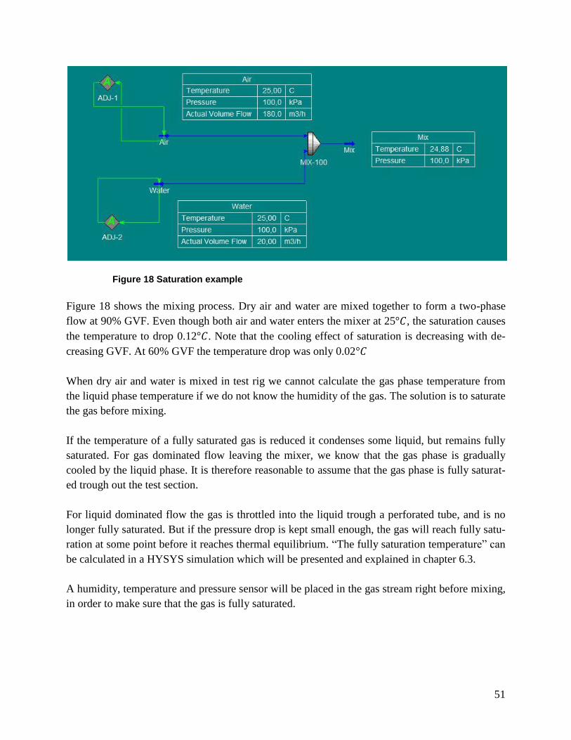
51
Figure 18 Saturation example
Figure 18 shows the mixing process. Dry air and water are mixed together to form a two-phase
flow at 90% GVF. Even though both air and water enters the mixer at 25 , the saturation causes
the temperature to drop 0.12 . Note that the cooling effect of saturation is decreasing with de-
creasing GVF. At 60% GVF the temperature drop was only 0.02
When dry air and water is mixed in test rig we cannot calculate the gas phase temperature from
the liquid phase temperature if we do not know the humidity of the gas. The solution is to saturate
the gas before mixing.
If the temperature of a fully saturated gas is reduced it condenses some liquid, but remains fully
saturated. For gas dominated flow leaving the mixer, we know that the gas phase is gradually
cooled by the liquid phase. It is therefore reasonable to assume that the gas phase is fully saturat-
ed trough out the test section.
For liquid dominated flow the gas is throttled into the liquid trough a perforated tube, and is no
longer fully saturated. But if the pressure drop is kept small enough, the gas will reach fully satu-
ration at some point before it reaches thermal equilibrium. “The fully saturation temperature” can
be calculated in a HYSYS simulation which will be presented and explained in chapter 6.3.
A humidity, temperature and pressure sensor will be placed in the gas stream right before mixing,
in order to make sure that the gas is fully saturated.
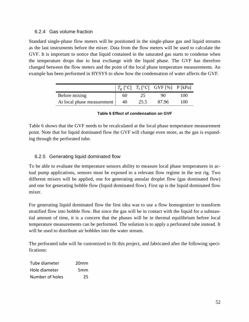
52
6.2.4 Gas volume fraction
Standard single-phase flow meters will be positioned in the single-phase gas and liquid streams
as the last instruments before the mixer. Data from the flow meters will be used to calculate the
GVF. It is important to notice that liquid contained in the saturated gas starts to condense when
the temperature drops due to heat exchange with the liquid phase. The GVF has therefore
changed between the flow meters and the point of the local phase temperature measurements. An
example has been performed in HYSYS to show how the condensation of water affects the GVF.
GVF [%] P [kPa]
Before mixing 60 25 90 100
At local phase measurement 40 25.5 87.96 100
Table 6 Effect of condensation on GVF
Table 6 shows that the GVF needs to be recalculated at the local phase temperature measurement
point. Note that for liquid dominated flow the GVF will change even more, as the gas is expand-
ing through the perforated tube.
6.2.5 Generating liquid dominated flow
To be able to evaluate the temperature sensors ability to measure local phase temperatures in ac-
tual pump applications, sensors must be exposed to a relevant flow regime in the test rig. Two
different mixers will be applied, one for generating annular droplet flow (gas dominated flow)
and one for generating bobble flow (liquid dominated flow). First up is the liquid dominated flow
mixer.
For generating liquid dominated flow the first idea was to use a flow homogenizer to transform
stratified flow into bobble flow. But since the gas will be in contact with the liquid for a substan-
tial amount of time, it is a concern that the phases will be in thermal equilibrium before local
temperature measurements can be performed. The solution is to apply a perforated tube instead. It
will be used to distribute air bobbles into the water stream.
The perforated tube will be customized to fit this project, and fabricated after the following speci-
fications:
Tube diameter 20mm
Hole diameter 5mm
Number of holes 25
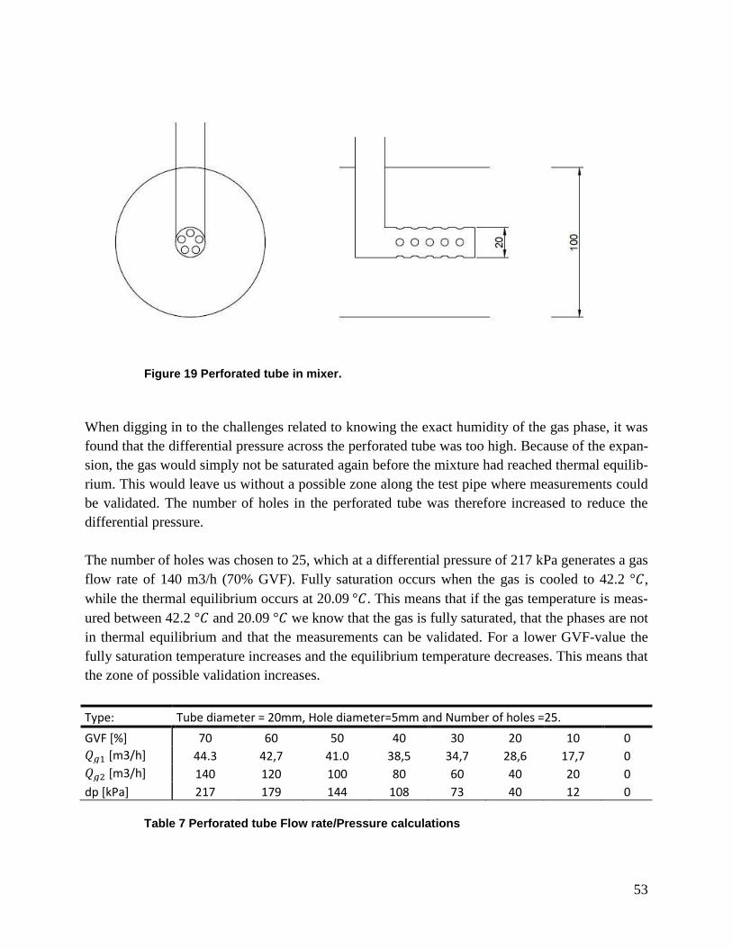
53
Figure 19 Perforated tube in mixer.
When digging in to the challenges related to knowing the exact humidity of the gas phase, it was
found that the differential pressure across the perforated tube was too high. Because of the expan-
sion, the gas would simply not be saturated again before the mixture had reached thermal equilib-
rium. This would leave us without a possible zone along the test pipe where measurements could
be validated. The number of holes in the perforated tube was therefore increased to reduce the
differential pressure.
The number of holes was chosen to 25, which at a differential pressure of 217 kPa generates a gas
flow rate of 140 m3/h (70% GVF). Fully saturation occurs when the gas is cooled to 42.2 ,
while the thermal equilibrium occurs at 20.09 . This means that if the gas temperature is meas-
ured between 42.2 and 20.09 we know that the gas is fully saturated, that the phases are not
in thermal equilibrium and that the measurements can be validated. For a lower GVF-value the
fully saturation temperature increases and the equilibrium temperature decreases. This means that
the zone of possible validation increases.
Type: Tube diameter = 20mm, Hole diameter=5mm and Number of holes =25.
GVF [%] 70 60 50 40 30 20 10 0
[m3/h] 44.3 42,7 41.0 38,5 34,7 28,6 17,7 0
[m3/h] 140 120 100 80 60 40 20 0
dp [kPa] 217 179 144 108 73 40 12 0
Table 7 Perforated tube Flow rate/Pressure calculations

54
Table 7 shows the differential pressure (dp) needed to get the correct gas flow rate. It also shows
the gas flow rate inn ( ) and out ( ) of the mixer. Because there is some uncertainty related
to when the flow will transform from liquid to gas domination, a differential pressure of more
than 217 kPa should be available. The same holds for differential pressure across the nozzles in
the next chapter.
6.2.6 Generating gas dominated flow
One or more nozzles will distribute water droplets into the mixer in order to generate a gas domi-
nated flow. The nozzle is chosen so that it provides the correct GVF range at the available liquid
pressure range. The droplet sizes can be reduced by increasing the number of nozzles. Two dif-
ferent options have been assessed.
The first option is to use a single nozzle in the centre of the stream. It can easily be operated by
adjusting the inlet pressure. One of the disadvantages is that the nozzle must be chosen so that it
can handle the whole range of GVFs from 50-90%. This mean that it either will need a very high
differential pressure to manage 50% GVF, or that it due to the low differential pressure will have
problems distributing the droplets at 90% GVF. Positioned in the centre of the pipe it will also
have substantial impact on the flow conditions.
Type: BETE NF 2250 303 Stainless steel
GVF [%] 90 80 70 60 50
QL [m3/h] 20 40 60 80 100
Number of Nozzles 1 1 1 1 1
Dp [bar] 0.4 1.7 3.8 6.8 10.6
Droplet sizes [μm] 22987 1949 1537 1289 1129
Table 8 Nozzle GVF calculations option 1
The second option applies two to ten smaller nozzles to generate different flow rates. This way,
the GVF range can be achieved while the differential pressure is kept moderate simply by varying
the amount of nozzles. A disadvantage is that it is more complicated to operate ten nozzles than
one.

55
Type: BETE NF 400 303 Stainless steel
GVF [%] 90 80 70 60 50
QL [m3/h] 20 40 60 80 100
Number of Nozzles 2 4 6 8 10
Dp [bar] 3.3 3.3 3.3 3.3 3.3
Droplet sizes [μm] 797 797 797 797 797
Table 9 Nozzle GVF calculations option 2
The single nozzle option will affect the flow more than a set of nozzles located near the pipe wall.
The combination of good positioning possibilities and constant differential pressure makes the
multiple nozzles option the best solution.
Figure 20 shows how the nozzles will be mounted to the pipe. The expansion of the pipe walls at
the nozzle mounting has three advantages:
Creates more space for mounting of the nozzles.
Less impact of the nozzles on the stream.
Droplets are sprayed in the flow direction.
The left drawing shows a cross-sectional view of the mixing device, while the right drawing
shows an axial view. The idea of the mounting is taken from a visual inspection of the wet gas
compressor rig at NTNU.
Figure 20 Nozzle mounting.

56
A large droplet contains more heat per unit surface than a smaller droplet, and it therefore re-
quires more time to reach the equilibrium temperature. The size and size distribution of the drop-
lets are expected to have an influence on the functionality of the sensors. Unfortunately no docu-
mentation on typical droplet sizes for multi-phase pumps or wet gas compressors have been
found. The calculated droplet sizes are displayed in Table 8 and Table 9.
6.3 Test procedure
This subchapter presents a complete test procedure that should be followed during tests. A simu-
lation environment in HYSYS representing the test rig will be used as a tool in the validation. A
screenshot of the simulation environment is displayed in Figure 21. For a better view, look to the
enlarged version of Figure 21 in Appendix D.
Values that will be measured during the tests are shown in the list below. They will be referred to
with their list reference in the rest of this subchapter. For example will the volumetric flow rate of
liquid before mixture be referred to as 2c. The measurement points can also be found in the
HYSYS simulation environment.
1. Saturated gas before mixing
a. Temperature
b. Pressure
c. Volumetric flow rate
d. Humidity
2. Liquid before mixing
a. Temperature
b. Pressure
c. Volumetric flow rate
3. Two-phase flow after mixing, but before thermal equilibrium
a. Gas Temperature
b. Liquid Temperature
c. Pressure
4. Two-phase flow equilibrium temperature 1
5. Two-phase flow equilibrium temperature 2
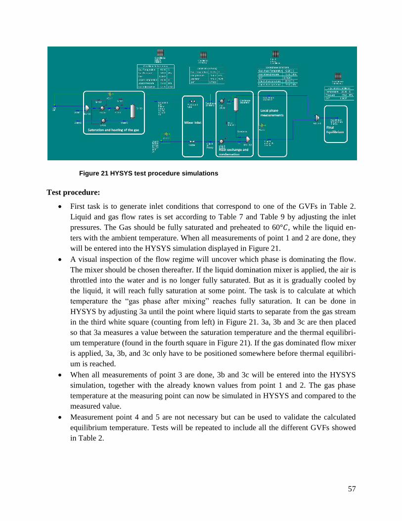
57
Figure 21 HYSYS test procedure simulations
Test procedure:
First task is to generate inlet conditions that correspond to one of the GVFs in Table 2.
Liquid and gas flow rates is set according to Table 7 and Table 9 by adjusting the inlet
pressures. The Gas should be fully saturated and preheated to 60 , while the liquid en-
ters with the ambient temperature. When all measurements of point 1 and 2 are done, they
will be entered into the HYSYS simulation displayed in Figure 21.
A visual inspection of the flow regime will uncover which phase is dominating the flow.
The mixer should be chosen thereafter. If the liquid domination mixer is applied, the air is
throttled into the water and is no longer fully saturated. But as it is gradually cooled by
the liquid, it will reach fully saturation at some point. The task is to calculate at which
temperature the “gas phase after mixing” reaches fully saturation. It can be done in
HYSYS by adjusting 3a until the point where liquid starts to separate from the gas stream
in the third white square (counting from left) in Figure 21. 3a, 3b and 3c are then placed
so that 3a measures a value between the saturation temperature and the thermal equilibri-
um temperature (found in the fourth square in Figure 21). If the gas dominated flow mixer
is applied, 3a, 3b, and 3c only have to be positioned somewhere before thermal equilibri-
um is reached.
When all measurements of point 3 are done, 3b and 3c will be entered into the HYSYS
simulation, together with the already known values from point 1 and 2. The gas phase
temperature at the measuring point can now be simulated in HYSYS and compared to the
measured value.
Measurement point 4 and 5 are not necessary but can be used to validate the calculated
equilibrium temperature. Tests will be repeated to include all the different GVFs showed
in Table 2.

58
Explanation of the simulation environment displayed in Figure 21:
The first with square simulates the heating and saturation process. Dry gas enters from the left.
The single phase heated and saturated gas before mixing can be found to the right of the first
square. The liquid before mixing can be found beneath it.
The second square simulates the mixing device. If the liquid domination mixer is applied the gas
stream is throttled, while the liquid is throttled when the gas domination mixer is applied. Gas
and liquid phase conditions directly after mixing, can be found between the second and the third
square. Note that no heat or mass transfer between the phases has accrued at this point.
The third square simulates heat and mass transfer between the phases that have occurred up-
stream of the local measurements (3a, 3b and 3c). The local measurements are found between the
third and fourth square. The final thermal equilibrium condition is found in the last square.
6.4 Sources of Error
Differences in bubble and droplet sizes will cause a temperature variation from bobble to bobble
and droplet to droplet as the heat exchange occurs at different rates, depending on the total mass
and the surface area. A liquid film will also have a different rate of heat transfer and may not
have the same temperature as the droplets travelling in the gas. The measured local phase tem-
perature is therefore not necessarily representative for the entire phase at the given position.
Heat loss through the wall along the pipe between the measured single phase temperatures and
the local phase temperatures is not included in the calculations. This uncertainty may cause a
difference between the calculated temperature and the measured temperature. Actual heat loss is
difficult to predict as the temperature profile is unknown. Isolation will therefore be used to keep
the heat transfer as low as possible.
Friction loss along the pipe between the measured single phase temperatures and the local phase
temperatures is not included in the calculations. A simulation has been run in HYSYS, and the
temperature rise in the test rig caused by friction loss where found to be insignificant, at least
compared to the accuracy of the applied sensors.
The focus of this thesis has been on temperature measurements. The accuracy of the pressure
measurements has not been assessed. The uncertainty related pressure measurements in multi-
phase flow might have a relevant influence on the calculated gas phase temperature.

59
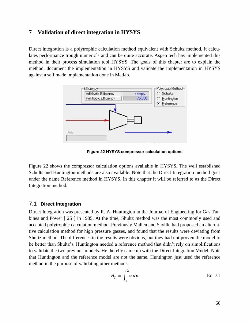
60
7 Validation of direct integration in HYSYS
Direct integration is a polytrophic calculation method equivalent with Schultz method. It calcu-
lates performance trough numeric`s and can be quite accurate. Aspen tech has implemented this
method in their process simulation tool HYSYS. The goals of this chapter are to explain the
method, document the implementation in HYSYS and validate the implementation in HYSYS
against a self made implementation done in Matlab.
Figure 22 HYSYS compressor calculation options
Figure 22 shows the compressor calculation options available in HYSYS. The well established
Schults and Huntington methods are also available. Note that the Direct Integration method goes
under the name Reference method in HYSYS. In this chapter it will be referred to as the Direct
Integration method.
7.1 Direct Integration
Direct Integration was presented by R. A. Huntington in the Journal of Engineering for Gas Tur-
bines and Power [ 25 ] in 1985. At the time, Shultz method was the most commonly used and
accepted polytrophic calculation method. Previously Mallen and Saville had proposed an alterna-
tive calculation method for high pressure gasses, and found that the results were deviating from
Shultz method. The differences in the results were obvious, but they had not proven the model to
be better than Shultz’s. Huntington needed a reference method that didn’t rely on simplifications
to validate the two previous models. He thereby came up with the Direct Integration Model. Note
that Huntington and the reference model are not the same. Huntington just used the reference
method in the purpose of validating other methods.
Eq. 7.1

61
Eq. 7.2
The direct integration model breaks the polytrophic compression path between two pressure lev-
els into several sub paths. Huntington states that if the compression path is divided sufficiently,
Eq. 7.1 could be linearized without significant error.
Eq. 7.3
Eq. 7.4
Eq. 7.5
Direct Integration can be applied to calculate outlet temperature of a pump or a turbine at a given
outlet pressure when the polytrophic efficiency is known. It can also be used to calculate poly-
trophic efficiency from test results when the outlet temperature and pressure is known. Either
way numerical calculation methods must be applied to equal Eq. 7.4 and Eq. 7.5. Today comput-
ers can easily solve the numeric task related to the Direct Integration Model. The Direct Integra-
tion Model is suggested to replace methods such as Shultz.
7.2 Implementation of direct integration in HYSYS
This chapter will look at how direct integration is implemented in HYSYS. The documentation
available in HYSYS simply refers to Huntington’s article [ 25 ]. It does not mention how many
steps the differential pressure is divided into, and not which iteration method or tolerance Aspen
Tech has applied. E-mail`s sent directly to Aspen Techs support office were never replied. And a
replied email sent through my supervisor did not answer the given questions. It has therefore
been difficult to establish any facts concerning the implementation.
Comparing Direct Integration Method in HYSYS to Schultz method in HYSYS revealed an in-
teresting discovery. As expected there is a deviation between the result of Schultz and Direct In-
tegration when calculating outlet temperature for a given polytrophic efficiency. But when calcu-
lating polytrophic efficiency from given inlet and outlet conditions, the two methods return the
exact same value. Two examples showing the discovery, is given in the tables below.

62
20 ⁰C
3000 kPa
4000 kPa
75 %
Table 10 Conditions
Method:
Schultz 24,4048343866527 ⁰C
Direct Integration HYSYS 24,4048155879620 ⁰C
Table 11 Outlet temperature calculations
Table 11 shows that when calculating outlet temperature with the conditions given in Table 10,
Schultz and Direct Integration returns different results. In the next example polytrophic efficiency
is calculated from given inlet and outlet conditions. The outlet conditions calculated with Schultz
method in the last example are inputs for the new example.
20 ⁰C
24,404834 ⁰C
3000 kPa
4000 kPa
Table 12 Conditions
Method:
Schultz 74,9998997648932 %
Direct Integration HYSYS 74,9998997648932 %
Table 13 Polytrophic efficiency calculations
Table 13 shows that when calculating polytrophic efficiency with the conditions given in Table
12, Schultz and Direct Integration returns the same results. This suggests that HYSYS uses the
same calculation method for both Schultz and Direct Integration when calculating polytrophic
efficiency.
Applying the direct integration for polytrophic efficiency calculations is much more complicated
and time consuming (will be further explained in the next subchapter). It is therefore reasonable
to believe that Aspen Tech hasn’t implemented Direct Integration for polytrophic efficiency cal-
culations, but simply applies Schultz instead.
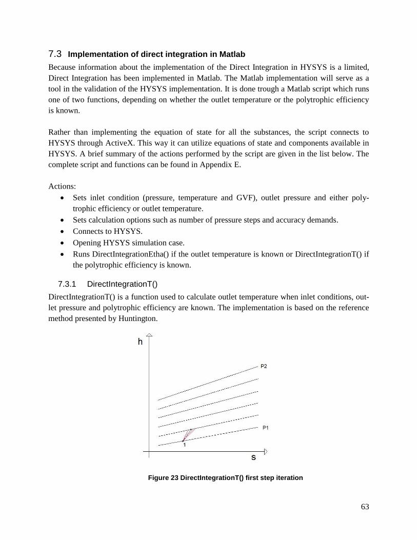
63
7.3 Implementation of direct integration in Matlab
Because information about the implementation of the Direct Integration in HYSYS is a limited,
Direct Integration has been implemented in Matlab. The Matlab implementation will serve as a
tool in the validation of the HYSYS implementation. It is done trough a Matlab script which runs
one of two functions, depending on whether the outlet temperature or the polytrophic efficiency
is known.
Rather than implementing the equation of state for all the substances, the script connects to
HYSYS through ActiveX. This way it can utilize equations of state and components available in
HYSYS. A brief summary of the actions performed by the script are given in the list below. The
complete script and functions can be found in Appendix E.
Actions:
Sets inlet condition (pressure, temperature and GVF), outlet pressure and either poly-
trophic efficiency or outlet temperature.
Sets calculation options such as number of pressure steps and accuracy demands.
Connects to HYSYS.
Opening HYSYS simulation case.
Runs DirectIntegrationEtha() if the outlet temperature is known or DirectIntegrationT() if
the polytrophic efficiency is known.
7.3.1 DirectIntegrationT()
DirectIntegrationT() is a function used to calculate outlet temperature when inlet conditions, out-
let pressure and polytrophic efficiency are known. The implementation is based on the reference
method presented by Huntington.
Figure 23 DirectIntegrationT() first step iteration

64
First it divides the differential pressure into a given number of steps and opens a stream from
HYSYS which corresponds to the given GVF. Then it calculates the conditions for each different
sub pressure level by applying the bisection iteration method to Eq. 7.4 and Eq. 7.5. Figure 23
shows how the conditions after the first step are calculated through iteration.
Figure 24 DirectIntegrationT() after last step iteration
When the bisection iteration method has found a solution to the conditions after the first step,
which meets the demands of accuracy, the results serve as inlet conditions for the next step. The
final compression path is formed, and the outlet temperature is calculated, when the conditions
after the last step has been decided (see the blue line in Figure 24). The red lines represent the
calculated outlet conditions that did not meet the demands of accuracy.
In theory the accuracy of the calculations will increase with the amount of calculation steps. But
since the data retrieved from HYSYS is limited to a certain amount of digits, the amount of steps
is limited as well. For very small steps, data from HYSYS starts to treat ∆p and ∆h as zero. Eq.
7.4 will then equal Eq. 7.5, even though the outlet temperature and polytrophic efficiency are
wrong. HYSYS is simply not accurate enough to cope with too many steps.
7.3.2 DirectIntegrationEtha()
DirectIntegrationEtha() is a function used to calculate the polytrophic efficiency when the inlet
and outlet temperatures and pressures are known. The implementation has an extra dimension
compared to DirectIntegration(T), as the polytrophic efficiency is not known. The function first
guess a polytrophic efficiency and then run the same procedure as in DirectIntegrationT(). When
the calculated outlet condition is found it is compared to the measured one. And a new poly-
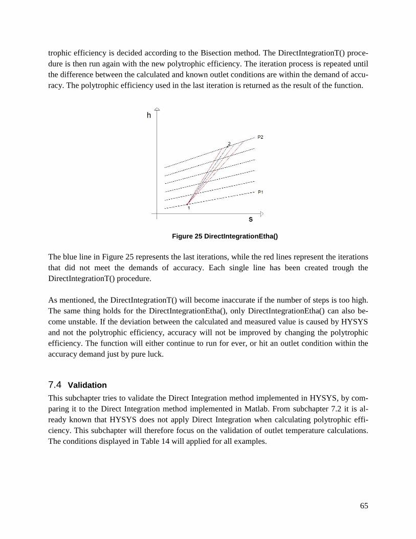
65
trophic efficiency is decided according to the Bisection method. The DirectIntegrationT() proce-
dure is then run again with the new polytrophic efficiency. The iteration process is repeated until
the difference between the calculated and known outlet conditions are within the demand of accu-
racy. The polytrophic efficiency used in the last iteration is returned as the result of the function.
Figure 25 DirectIntegrationEtha()
The blue line in Figure 25 represents the last iterations, while the red lines represent the iterations
that did not meet the demands of accuracy. Each single line has been created trough the
DirectIntegrationT() procedure.
As mentioned, the DirectIntegrationT() will become inaccurate if the number of steps is too high.
The same thing holds for the DirectIntegrationEtha(), only DirectIntegrationEtha() can also be-
come unstable. If the deviation between the calculated and measured value is caused by HYSYS
and not the polytrophic efficiency, accuracy will not be improved by changing the polytrophic
efficiency. The function will either continue to run for ever, or hit an outlet condition within the
accuracy demand just by pure luck.
7.4 Validation
This subchapter tries to validate the Direct Integration method implemented in HYSYS, by com-
paring it to the Direct Integration method implemented in Matlab. From subchapter 7.2 it is al-
ready known that HYSYS does not apply Direct Integration when calculating polytrophic effi-
ciency. This subchapter will therefore focus on the validation of outlet temperature calculations.
The conditions displayed in Table 14 will applied for all examples.

66
20 ⁰C
3000 kPa
4000 kPa
75 %
Table 14 Conditions
Calculated outlet temperatures for a typical hydro carbon mixture at 60% GVF can be found in
Table 15. The temperatures are calculated from Schultz model in HYSYS, Direct Integration
model in HYSYS and the Direct Integration Model implemented in Matlab. The tolerance in the
Matlab implementation is set so low that a decrease in tolerance would not affect the results with-
in the amount of digits displayed in Table 15.
Method:
HYSYS Compressor Schultz 24,404834 ⁰C
HYSYS Compressor Direct Integration 24,404815 ⁰C
Matlab Direct Integration (1 step) 24.383473 ⁰C
Matlab Direct Integration (2 steps) 24.361063 ⁰C
Matlab Direct Integration (5 steps) 24.354671 ⁰C
Matlab Direct Integration (10 steps) 24.353754 ⁰C
Matlab Direct Integration (20 steps) 24.353524 ⁰C
Table 15 Outlet temperature calculations of a hydrocarbon mixture at 60% GVF
The purpose of this example was to decide how many steps HYSYS applies in the implementa-
tion of Direct Integration. The Matlab implementation was run with different amount of pressure
steps without closing in on the HYSYS implementation. The deviation can therefore not be
caused just by different number of steps.
If the difference between the Direct Integration Model in HYSYS and Matlab is not caused by a
difference in the number of steps, it can only be caused by a difference in tolerance limits. The
example above was repeated for numerous of different conditions, and the results were the same.
The direct Integration method in HYSYS was always closer to Schults than to the Direct Integra-
tion method implemented in Matlab. It is difficult to say much about what kind of tolerance
HYSYS uses. But high tolerance would not generate a systematic inaccuracy in the direction of
Shultz. It would be a random inaccuracy occurring on both sides of the Direct Integration Matlab
results.
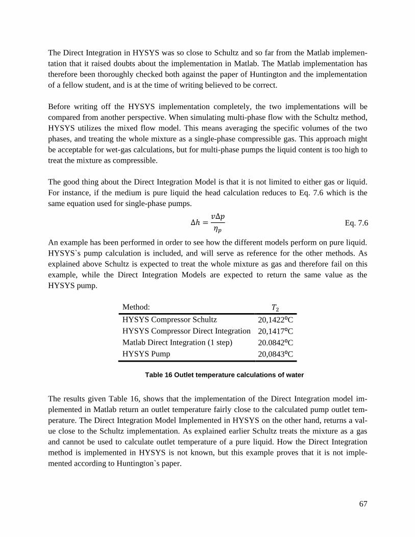
67
The Direct Integration in HYSYS was so close to Schultz and so far from the Matlab implemen-
tation that it raised doubts about the implementation in Matlab. The Matlab implementation has
therefore been thoroughly checked both against the paper of Huntington and the implementation
of a fellow student, and is at the time of writing believed to be correct.
Before writing off the HYSYS implementation completely, the two implementations will be
compared from another perspective. When simulating multi-phase flow with the Schultz method,
HYSYS utilizes the mixed flow model. This means averaging the specific volumes of the two
phases, and treating the whole mixture as a single-phase compressible gas. This approach might
be acceptable for wet-gas calculations, but for multi-phase pumps the liquid content is too high to
treat the mixture as compressible.
The good thing about the Direct Integration Model is that it is not limited to either gas or liquid.
For instance, if the medium is pure liquid the head calculation reduces to Eq. 7.6 which is the
same equation used for single-phase pumps.
Eq. 7.6
An example has been performed in order to see how the different models perform on pure liquid.
HYSYS`s pump calculation is included, and will serve as reference for the other methods. As
explained above Schultz is expected to treat the whole mixture as gas and therefore fail on this
example, while the Direct Integration Models are expected to return the same value as the
HYSYS pump.
Method:
HYSYS Compressor Schultz 20,1422⁰C
HYSYS Compressor Direct Integration 20,1417⁰C
Matlab Direct Integration (1 step) 20.0842⁰C
HYSYS Pump 20,0843⁰C
Table 16 Outlet temperature calculations of water
The results given Table 16, shows that the implementation of the Direct Integration model im-
plemented in Matlab return an outlet temperature fairly close to the calculated pump outlet tem-
perature. The Direct Integration Model Implemented in HYSYS on the other hand, returns a val-
ue close to the Schultz implementation. As explained earlier Schultz treats the mixture as a gas
and cannot be used to calculate outlet temperature of a pure liquid. How the Direct Integration
method is implemented in HYSYS is not known, but this example proves that it is not imple-
mented according to Huntington`s paper.

68
8 Influence of heavy components on the performance calculations
The performance of a multi-phase pump is affected by the properties of the fluid. If the fluid is a
Hydrocarbon mixture, the composition is decided trough an analysis of the mixture. The cost of
the analysis is increasing with the amount of hydrocarbons considered. To reduce costs, industry
actors sometimes tend to neglect the heavier components. This chapter will investigate the im-
portance of including heavy components in the calculations and explain the consequences of ne-
glecting them. Examples will be performed and the results will show the effects on performance
parameters and compression path.
Direct Integration is chosen as the calculation method. Earlier chapters of this thesis have shown
that the Direct Integration method implemented in HYSYS, do not perform the calculation such
as Huntington intended. Another drawback with the simulations in HYSYS is that it does not
display the compression path, only inlet and outlet conditions. The direct integration model im-
plemented in Matlab will therefore be used instead. The Matlab implementation can return all
data related to the compression path, and the method is believed to be more correct.
8.1 Compositions
To be able to study the effects of neglecting some parts of the composition two different mixtures
will be compared. The first mixture (A) represents the actual fluid composition and contains Ni-
trogen, CO2 and hydrocarbons from C1 to C30. The second mixture (B) represents the results
from a low-cost analysis performed on the first mixture. It contains the same amount of Nitrogen,
CO2 and hydrocarbons from C1 to C9, while C10-C30 are considered as C10+.
Table 17 presents actual fluid compositions and low cost analyzes for 90, 60, 30 and 0% GVF
mixtures. The compositions are generated from a typically wet-gas case, handed over to me by
my supervisor. The compositions in Table 17 representing the different GVFs were generated by
extracting some of the lighter components. The GVF is calculated at a temperature of 5 ⁰C and at
a pressure of 3000 kPa.

69
GVF: 90% 60% 30% 0%
Composition: A B A B A B A B
Nitrogen 0,0004 0,0004 0,0002 0,0002 0,0002 0,0002 0,0002 0,0002
CO2 0,0259 0,0259 0,0162 0,0162 0,0103 0,0103 0,0065 0,0065
Methane 0,5029 0,5029 0,2686 0,2686 0,1944 0,1944 0,1475 0,1475
Ethane 0,1738 0,1738 0,1445 0,1445 0,0941 0,0941 0,0576 0,0576
Propane 0,0818 0,0818 0,1240 0,1240 0,1024 0,1024 0,0640 0,0640
i-Butane 0,0139 0,0139 0,0262 0,0262 0,0277 0,0277 0,0207 0,0207
n-Butane 0,0250 0,0250 0,0490 0,0490 0,0558 0,0558 0,0453 0,0453
i-Pentane 0,0149 0,0149 0,0307 0,0307 0,0396 0,0396 0,0401 0,0401
n-Pentane 0,0141 0,0141 0,0294 0,0294 0,0388 0,0388 0,0416 0,0416
n-Hexane 0,0187 0,0187 0,0395 0,0395 0,0546 0,0546 0,0675 0,0675
n-Heptane 0,0290 0,0290 0,0614 0,0614 0,0860 0,0860 0,1123 0,1123
n-Octane 0,0283 0,0283 0,0598 0,0598 0,0840 0,0840 0,1119 0,1119
n-Nonane 0,0134 0,0134 0,0283 0,0283 0,0398 0,0398 0,0533 0,0533
n-Decane/C10+ 0,0120 0,0579 0,0254 0,1223 0,0357 0,1722 0,0480 0,2315
n-C11 0,0073
0,0154
0,0216
0,0290
n-C12 0,0065
0,0137
0,0193
0,0260
n-C13 0,0057
0,0121
0,0171
0,0229
n-C14 0,0054
0,0113
0,0159
0,0214
n-C15 0,0042
0,0089
0,0125
0,0168
n-C16 0,0031
0,0065
0,0091
0,0122
n-C17 0,0027
0,0057
0,0080
0,0107
n-C18 0,0023
0,0049
0,0068
0,0092
n-C19 0,0019
0,0040
0,0057
0,0076
n-C20 0,0015
0,0032
0,0045
0,0061
n-C21 0,0011
0,0024
0,0034
0,0046
n-C22 0,0008
0,0016
0,0023
0,0031
n-C23 0,0008
0,0016
0,0023
0,0031
n-C24 0,0004
0,0008
0,0011
0,0015
n-C25 0,0004
0,0008
0,0011
0,0015
n-C26 0,0004
0,0008
0,0011
0,0015
n-C27 0,0004
0,0008
0,0011
0,0015
n-C28 0,0004
0,0008
0,0011
0,0015
n-C29 0,0004
0,0008
0,0011
0,0015
n-C30 0,0004
0,0008
0,0011
0,0015
Table 17 Hydrocarbon composition Actual mixtures VS Low cost analyzes
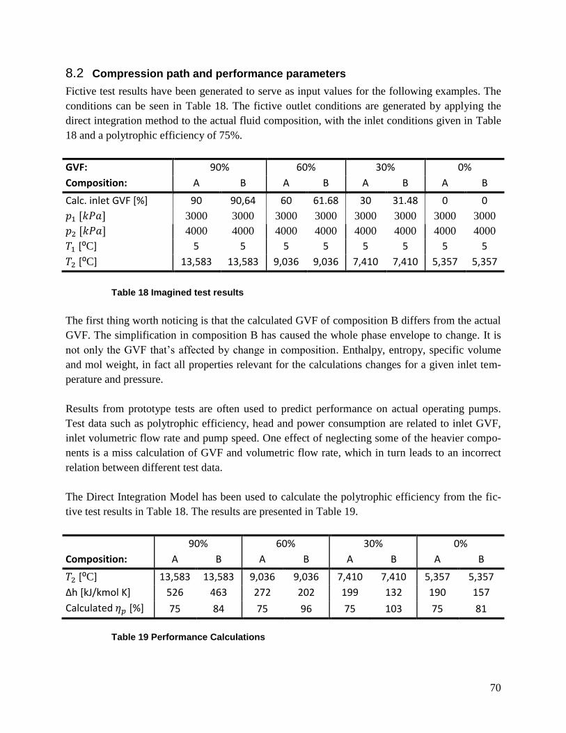
70
8.2 Compression path and performance parameters
Fictive test results have been generated to serve as input values for the following examples. The
conditions can be seen in Table 18. The fictive outlet conditions are generated by applying the
direct integration method to the actual fluid composition, with the inlet conditions given in Table
18 and a polytrophic efficiency of 75%.
GVF: 90% 60% 30% 0%
Composition: A B A B A B A B
Calc. inlet GVF [%] 90 90,64 60 61.68 30 31.48 0 0
3000 3000 3000 3000 3000 3000 3000 3000
4000 4000 4000 4000 4000 4000 4000 4000
[⁰C] 5 5 5 5 5 5 5 5
[⁰C] 13,583 13,583 9,036 9,036 7,410 7,410 5,357 5,357
Table 18 Imagined test results
The first thing worth noticing is that the calculated GVF of composition B differs from the actual
GVF. The simplification in composition B has caused the whole phase envelope to change. It is
not only the GVF that’s affected by change in composition. Enthalpy, entropy, specific volume
and mol weight, in fact all properties relevant for the calculations changes for a given inlet tem-
perature and pressure.
Results from prototype tests are often used to predict performance on actual operating pumps.
Test data such as polytrophic efficiency, head and power consumption are related to inlet GVF,
inlet volumetric flow rate and pump speed. One effect of neglecting some of the heavier compo-
nents is a miss calculation of GVF and volumetric flow rate, which in turn leads to an incorrect
relation between different test data.
The Direct Integration Model has been used to calculate the polytrophic efficiency from the fic-
tive test results in Table 18. The results are presented in Table 19.
90% 60% 30% 0%
Composition: A B A B A B A B
[⁰C] 13,583 13,583 9,036 9,036 7,410 7,410 5,357 5,357
∆h [kJ/kmol K] 526 463 272 202 199 132 190 157
Calculated [%] 75 84 75 96 75 103 75 81
Table 19 Performance Calculations

71
Table 19 shows that the calculated polytrophic efficiency for composition B deviates from the
actual polytrophic efficiency. The head deviation is also comprehensive. From chapter 4 we
know that the head degradation factor is calculated from the single and two-phase head. From Eq.
8.1 it is evident that two-phase performance predictions will be affected by a simplification of the
composition.
Eq. 8.1
The compression paths from the examples in Table 19 will now be presented in a numerous of h-
s diagrams. Because of the differences in fluid properties of composition A and B, they are not
plotted in the same graph.
Figure 26 Direct integration, Composition A VS B, Number of steps = 10, GVF 90%.
First up is the 90% GVF example. The graph to the left in Figure 26 shows the compression path
at 90% GVF of the actual composition. The compression path of the simplified composition is
plotted in the graph to the right. Figure 26 show that the simplification of the composition causes
an inaccuracy in the inlet enthalpy and entropy. The increased polytrophic efficiency found in
Table 19 can be seen in the right figure as an increase of steepness of the compression path.
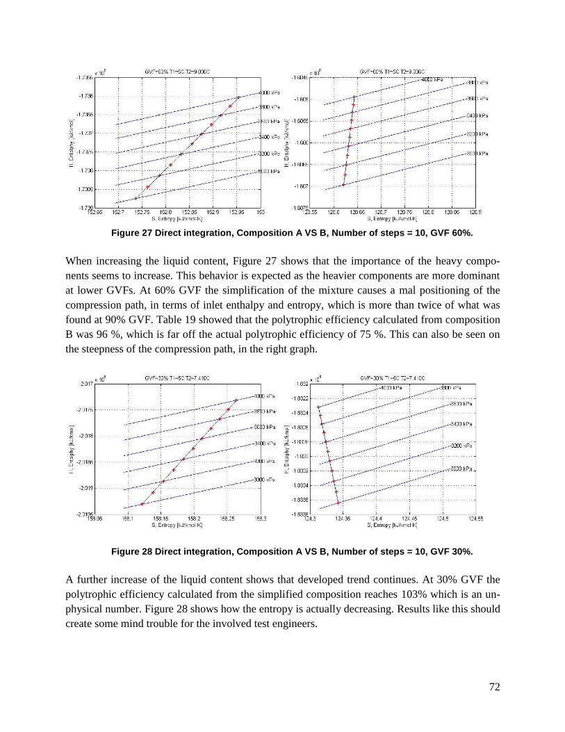
72
Figure 27 Direct integration, Composition A VS B, Number of steps = 10, GVF 60%.
When increasing the liquid content, Figure 27 shows that the importance of the heavy compo-
nents seems to increase. This behavior is expected as the heavier components are more dominant
at lower GVFs. At 60% GVF the simplification of the mixture causes a mal positioning of the
compression path, in terms of inlet enthalpy and entropy, which is more than twice of what was
found at 90% GVF. Table 19 showed that the polytrophic efficiency calculated from composition
B was 96 %, which is far off the actual polytrophic efficiency of 75 %. This can also be seen on
the steepness of the compression path, in the right graph.
Figure 28 Direct integration, Composition A VS B, Number of steps = 10, GVF 30%.
A further increase of the liquid content shows that developed trend continues. At 30% GVF the
polytrophic efficiency calculated from the simplified composition reaches 103% which is an un-
physical number. Figure 28 shows how the entropy is actually decreasing. Results like this should
create some mind trouble for the involved test engineers.
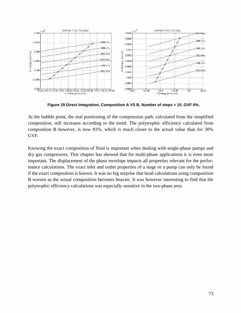
73
Figure 29 Direct integration, Composition A VS B, Number of steps = 10, GVF 0%.
At the bubble point, the mal positioning of the compression path, calculated from the simplified
composition, still increases according to the trend. The polytrophic efficiency calculated from
composition B however, is now 81%, which is much closer to the actual value than for 30%
GVF.
Knowing the exact composition of fluid is important when dealing with single-phase pumps and
dry gas compressors. This chapter has showed that for multi-phase applications it is even more
important. The displacement of the phase envelope impacts all properties relevant for the perfor-
mance calculations. The exact inlet and outlet properties of a stage or a pump can only be found
if the exact composition is known. It was no big surprise that head calculations using composition
B worsen as the actual composition becomes heavier. It was however interesting to find that the
polytrophic efficiency calculations was especially sensitive in the two-phase area.

74
9 Conclusions and Suggestions to Further Work
Because the heat capacity per unit volume of a liquid is much higher than the heat capacity per
unit volume of a gas, the temperature increase is limited in the whole GVF range of Multi-phase
pumps (0-90%GVF). In the lower GVF range the temperature increase is in fact so small that the
common practice in the industry is to simplify calculations by assuming an isothermal compres-
sion process. In the higher GVF region (60-90%GVF) the isothermal calculations becomes inac-
curate. Polytrophic calculations can provide accurate calculations, but is highly sensitive to the
accuracy of the temperature measurements, especially for the liquid phase. For the gas phase a
sensitivity analysis performed in this thesis has showed that temperature measurements can be
less accurate, due to a lower heat capacity.
The implementation of the Direct Integration method in HYSYS is not found to be implemented
according to the Reference Method presented by Huntington. For polytrophic efficiency calcula-
tions it does not seem to be implemented at all. If Direct Integration is to be used in future per-
formance calculations, better results will be achieved by applying the Matlab implementation
presented in this thesis.
It was found that accurate performance calculations depend on accurate determination of the
composition. The calculations of polytrophic efficiency showed to be especially sensitive when
operating far into the two-phase area. Both when analyzing test results and predicting perfor-
mance of a subsea pump, engineers needs to acknowledge the importance of the fluid composi-
tion.
Suggestions for further work
A sensitivity analysis of all the measured parameters connected to the calculation of the local gas
temperature in the test rig should be conducted. Due to the time limit of this thesis, sensitivity
analyzes has so far only been done on the temperature measurements.
After the sensitivity analyzes has been performed, the tests should be carried out. Results will
show whether or not the accuracy of the different concepts presented in Chapter 6.2.2 are high
enough.
If the tests show that measurements of the local gas phase is possible and that the accuracy is
found high enough, the next step is to look at how the concepts can be moved into an actual
pump application. Challenges like positioning and durability will have to be tackled.

75
Collaboration with AspenTech should be established in order to clarify how their reference meth-
od is implemented in HYSYS. If their implementation is found incorrect, AspenTech should be
encouraged to improve their version of the reference method. Calculation options such as number
of pressure steps and tolerance levels should be included in the user interface.
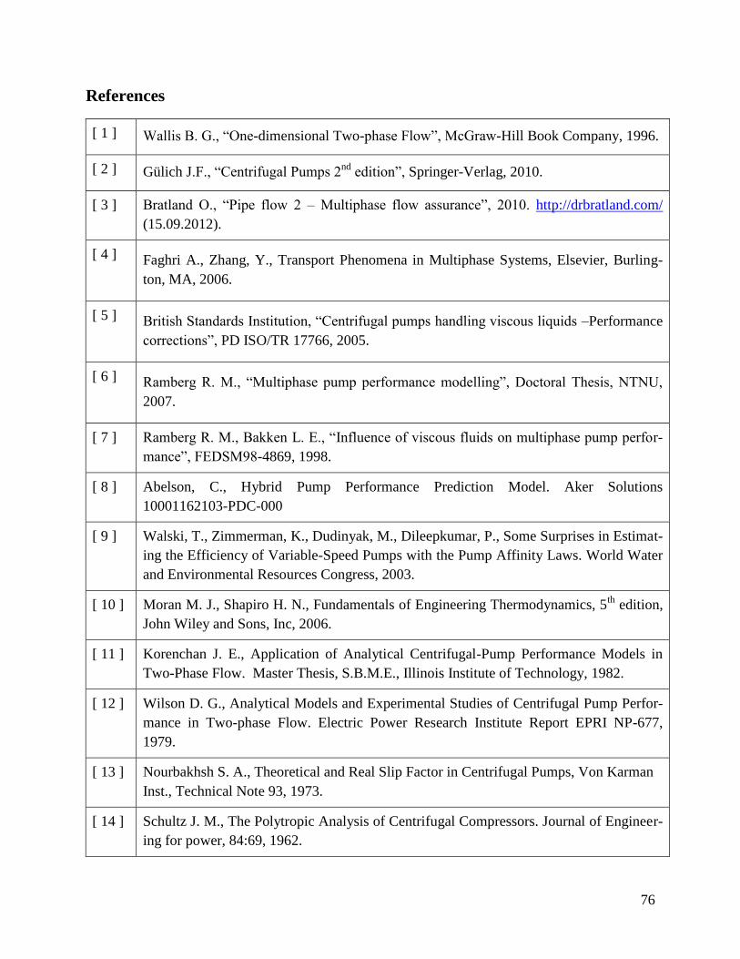
76
References
[ 1 ] Wallis B. G., “One-dimensional Two-phase Flow”, McGraw-Hill Book Company, 1996.
[ 2 ] Gülich J.F., “Centrifugal Pumps 2nd
edition”, Springer-Verlag, 2010.
[ 3 ] Bratland O., “Pipe flow 2 – Multiphase flow assurance”, 2010. http://drbratland.com/
(15.09.2012).
[ 4 ]
Faghri A., Zhang, Y., Transport Phenomena in Multiphase Systems, Elsevier, Burling-
ton, MA, 2006.
[ 5 ]
British Standards Institution, “Centrifugal pumps handling viscous liquids –Performance
corrections”, PD ISO/TR 17766, 2005.
[ 6 ]
Ramberg R. M., “Multiphase pump performance modelling”, Doctoral Thesis, NTNU,
2007.
[ 7 ] Ramberg R. M., Bakken L. E., “Influence of viscous fluids on multiphase pump perfor-
mance”, FEDSM98-4869, 1998.
[ 8 ] Abelson, C., Hybrid Pump Performance Prediction Model. Aker Solutions
10001162103-PDC-000
[ 9 ] Walski, T., Zimmerman, K., Dudinyak, M., Dileepkumar, P., Some Surprises in Estimat-
ing the Efficiency of Variable-Speed Pumps with the Pump Affinity Laws. World Water
and Environmental Resources Congress, 2003.
[ 10 ] Moran M. J., Shapiro H. N., Fundamentals of Engineering Thermodynamics, 5th
edition,
John Wiley and Sons, Inc, 2006.
[ 11 ] Korenchan J. E., Application of Analytical Centrifugal-Pump Performance Models in
Two-Phase Flow. Master Thesis, S.B.M.E., Illinois Institute of Technology, 1982.
[ 12 ] Wilson D. G., Analytical Models and Experimental Studies of Centrifugal Pump Perfor-
mance in Two-phase Flow. Electric Power Research Institute Report EPRI NP-677,
1979.
[ 13 ] Nourbakhsh S. A., Theoretical and Real Slip Factor in Centrifugal Pumps, Von Karman
Inst., Technical Note 93, 1973.
[ 14 ] Schultz J. M., The Polytropic Analysis of Centrifugal Compressors. Journal of Engineer-
ing for power, 84:69, 1962.

77
[ 15 ] Murakami M., Minemura K., Effects of Entrained Air on the Performance of a Centrifu-
gal Pump, JSME, Vol. 17, No 110, August, 1974.
[ 16 ] Test report, High Viscosity Fluid Pump Test PAZFLOR PROJECT. Aker Solutions,
10000104797.
[ 17 ] Knudsen H., MultiBooster Performance, Project Thesis, Norwegian University of Sci-
ence, 2012.
[ 18 ] Gié P., Buvat P., Bratau C., Durando P., Poseidon Multiphase Pump: Field Tests Results.
Offshore Techn Conf OTC 7037, 4 (1992), 489-501
[ 19 ] API 610, Centrifugal Pumps for Petroleum, Petrochemical and Natural Gas Industries.
Eleventh Edition, September 2010
[ 20 ] Turbo compressors – Performance test code. ISO 5389:2005, Geneva, Switzerland,
2005.
[ 21 ] Hunseid Ø., Bakken L. E., Evaluation of Performance Models for Wet Gas Compressors.
Doctoral Thesis, Norwegian University of Science, 2008
[ 22 ] Saravanamutto H.I.H., Rogers G.F.C., Cohen H. Gas Turbine Theory. Pearson Educa-
tion, 6th
edition, 2009.
[ 23 ] Falcimagine J., Decarre S., Multiphase Production. IFP Publications, Paris 2008. ISBN
978-27108-0913-5
[ 24 ] Ripka P., Tipek A., Modern Sensors Handbook, ISTE, 2007.
[ 25 ] Huntington R. A., Evaluation of Polytrophic Calculation Methods for Turbo machinery
Performance, Journal of Engineering for Gas Turbines and Power, October 1985, Vol.
107.
[ 26 ] Mallen M., Saville G., Polytrophic Processes in the Performance Prediction of Centrifu-
gal Compressors, Institute of Mechanical Engineers, Paper No. C183, pp 89-96.
[ 27 ] Schleicher E., Da Silva M. J., Hampel U., Enhanced Local Void and Temperature Meas-
urements for Highly Transient Multiphase Flows, IEE Transactions on Instrumentation
and Mesurement, Vol. 57, No. 2, February 2008.
[ 28 ] Consolation with Arne Veland FRAMO Engineering AS
[ 29 ] Taitel Y., Duckler A. E., A Model for Predicting Flow Regime Transitions in Horizontal
and Near Horizontal Gas-Liquid Flow. AIChE Journal, 22/1.

78
[ 30 ] Standard Specification for Industrial Platinum Resistance Thermometers,
E1137/E1137M, American Society for Testing and Materials, 2008.
[ 31 ] White F. M., Fluid Mechanics, Sixth Edition, University of Rhode Island, McGrawHill
Higher Education.

79

80
Appendix
A - Offer on Thermo-Needle Probe System
B - Data Sheets
C - Liquid Dominated Mixer Calculations
D - Simulation Environment Test Rig
E - Matlab Implementation of Direct Integration
F - Direct Integration Results

81

82
A - Offer on Thermo-Needle-Probe System

83

84
B - Data Sheets
Sea-bird Electronics SBE 38
BETE NF Standard Fan Nozzle
GEVACRIL Plexiglas Pipe

85

86
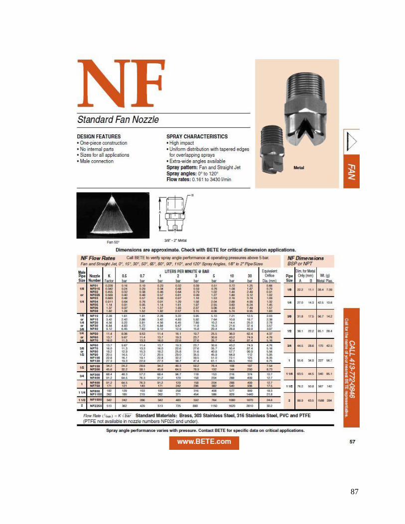
87

88

89
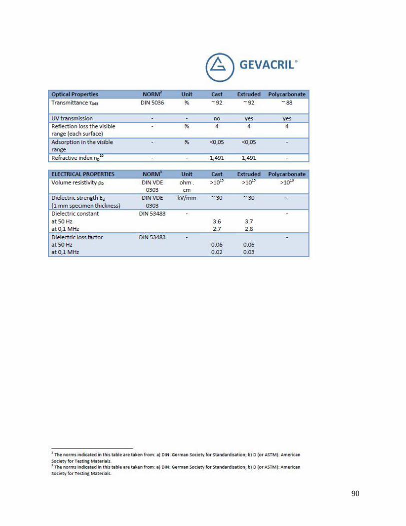
90

91
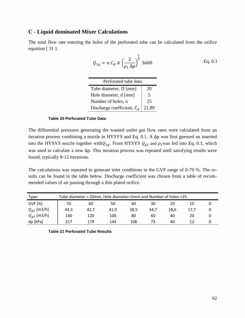
92
C - Liquid dominated Mixer Calculations
The total flow rate entering the holes of the perforated tube can be calculated from the orifice
equation [ 31 ].
Eq. 0.1
Perforated tube data
Tube diameter, D [mm] 20
Hole diameter, d [mm] 5
Number of holes, n 25
Discharge coefficient, 21,89
Table 20 Perforated Tube Data
The differential pressures generating the wanted outlet gas flow rates were calculated from an
iteration process combining a nozzle in HYSYS and Eq. 0.1. A ∆p was first guessed an inserted
into the HYSYS nozzle together with . From HYSYS and was fed into Eq. 0.1, which
was used to calculate a new ∆p. This iteration process was repeated until satisfying results were
found, typically 8-12 iterations.
The calculations was repeated to generate inlet conditions in the GVF range of 0-70 %. The re-
sults can be found in the table below. Discharge coefficient was chosen from a table of recom-
mended values of air passing through a thin plated orifice.
Type: Tube diameter = 20mm, Hole diameter=5mm and Number of holes =25.
GVF [%] 70 60 50 40 30 20 10 0
[m3/h] 44.3 42,7 41.0 38,5 34,7 28,6 17,7 0
[m3/h] 140 120 100 80 60 40 20 0
dp [kPa] 217 179 144 108 73 40 12 0 Table 21 Perforated Tube Results

93

94
D - Simulation Environment Test Rig

95
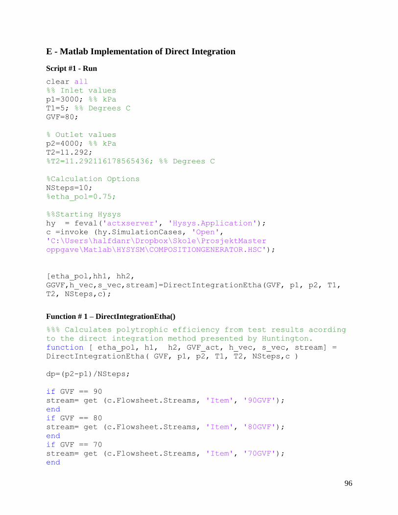
96
E - Matlab Implementation of Direct Integration
Script #1 - Run
clear all
%% Inlet values
p1=3000; %% kPa
T1=5; %% Degrees C
GVF=80;
% Outlet values
p2=4000; %% kPa
T2=11.292;
%T2=11.292116178565436; %% Degrees C
%Calculation Options
NSteps=10;
%etha_pol=0.75;
%%Starting Hysys
hy = feval('actxserver', 'Hysys.Application');
c =invoke (hy.SimulationCases, 'Open',
'C:\Users\halfdanr\Dropbox\Skole\ProsjektMaster
oppgave\Matlab\HYSYSM\COMPOSITIONGENERATOR.HSC');
[etha_pol,hh1, hh2,
GGVF,h_vec,s_vec,stream]=DirectIntegrationEtha(GVF, p1, p2, T1,
T2, NSteps,c);
Function # 1 – DirectIntegrationEtha()
%%% Calculates polytrophic efficiency from test results acording
to the direct integration method presented by Huntington.
function [ etha_pol, h1, h2, GVF_act, h_vec, s_vec, stream] =
DirectIntegrationEtha( GVF, p1, p2, T1, T2, NSteps,c )
dp=(p2-p1)/NSteps;
if GVF == 90
stream= get (c.Flowsheet.Streams, 'Item', '90GVF');
end
if GVF == 80
stream= get (c.Flowsheet.Streams, 'Item', '80GVF');
end
if GVF == 70
stream= get (c.Flowsheet.Streams, 'Item', '70GVF');
end
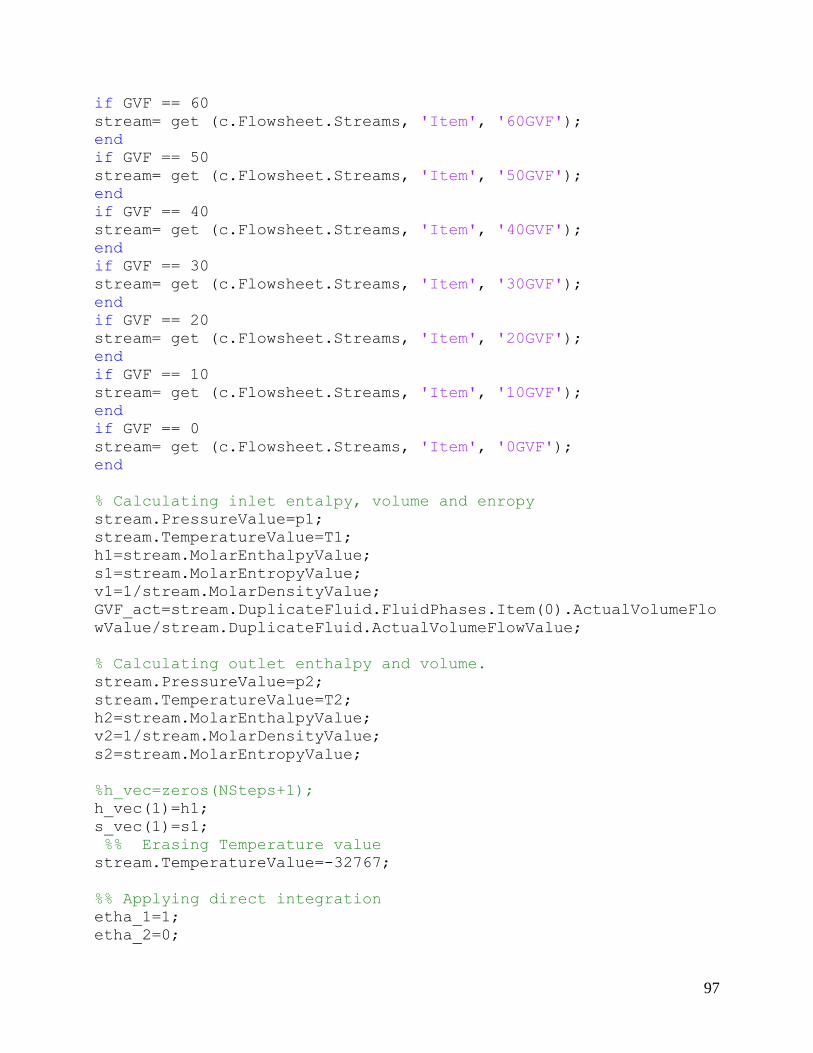
97
if GVF == 60
stream= get (c.Flowsheet.Streams, 'Item', '60GVF');
end
if GVF == 50
stream= get (c.Flowsheet.Streams, 'Item', '50GVF');
end
if GVF == 40
stream= get (c.Flowsheet.Streams, 'Item', '40GVF');
end
if GVF == 30
stream= get (c.Flowsheet.Streams, 'Item', '30GVF');
end
if GVF == 20
stream= get (c.Flowsheet.Streams, 'Item', '20GVF');
end
if GVF == 10
stream= get (c.Flowsheet.Streams, 'Item', '10GVF');
end
if GVF == 0
stream= get (c.Flowsheet.Streams, 'Item', '0GVF');
end
% Calculating inlet entalpy, volume and enropy
stream.PressureValue=p1;
stream.TemperatureValue=T1;
h1=stream.MolarEnthalpyValue;
s1=stream.MolarEntropyValue;
v1=1/stream.MolarDensityValue;
GVF_act=stream.DuplicateFluid.FluidPhases.Item(0).ActualVolumeFlo
wValue/stream.DuplicateFluid.ActualVolumeFlowValue;
% Calculating outlet enthalpy and volume.
stream.PressureValue=p2;
stream.TemperatureValue=T2;
h2=stream.MolarEnthalpyValue;
v2=1/stream.MolarDensityValue;
s2=stream.MolarEntropyValue;
%h_vec=zeros(NSteps+1);
h_vec(1)=h1;
s_vec(1)=s1;
%% Erasing Temperature value
stream.TemperatureValue=-32767;
%% Applying direct integration
etha_1=1;
etha_2=0;

98
while abs(etha_1-etha_2) >= 1e-4
etha_pol=(etha_1+etha_2)/2;
p_start=p1;
h_start=h1;
v_start=v1;
for n=1:1:NSteps
p_end=p_start+dp;
Itt1=0;
Itt2=etha_pol*(h2-h1)*2;
while abs(Itt1-Itt2)>1e-4
Itt=(Itt1+Itt2)/2;
h_end=Itt/etha_pol+h_start;
stream.MolarEnthalpyValue=h_end;
stream.PressureValue=p_end;
v_end=1/stream.MolarDensityValue;
v_avg=(v_start+v_end)/2;
reff=v_avg*dp;
if reff>=Itt
Itt1=Itt;s
else
Itt2=Itt;
end
end
h_start=h_end;
p_start=p_end;
v_start=v_end;
h_vec(n+1)=h_end;
s_vec(n+1)=stream.molarEntropyValue;
end
h2_end=h_end;
stream.MolarEnthalpyValue=h_end;
stream.PressureValue=p_end;
T2_end=stream.TemperatureValue;
if T2_end >= T2
etha_2 = etha_pol;
else
etha_1 = etha_pol;
end
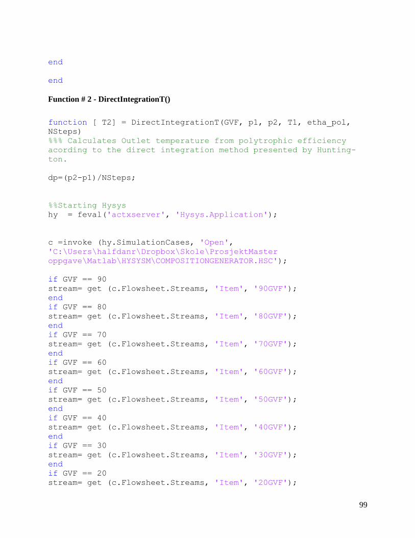
99
end
end
Function # 2 - DirectIntegrationT()
function [ T2] = DirectIntegrationT(GVF, p1, p2, T1, etha_pol,
NSteps)
%%% Calculates Outlet temperature from polytrophic efficiency
acording to the direct integration method presented by Hunting-
ton.
dp=(p2-p1)/NSteps;
%%Starting Hysys
hy = feval('actxserver', 'Hysys.Application');
c =invoke (hy.SimulationCases, 'Open',
'C:\Users\halfdanr\Dropbox\Skole\ProsjektMaster
oppgave\Matlab\HYSYSM\COMPOSITIONGENERATOR.HSC');
if GVF == 90
stream= get (c.Flowsheet.Streams, 'Item', '90GVF');
end
if GVF == 80
stream= get (c.Flowsheet.Streams, 'Item', '80GVF');
end
if GVF == 70
stream= get (c.Flowsheet.Streams, 'Item', '70GVF');
end
if GVF == 60
stream= get (c.Flowsheet.Streams, 'Item', '60GVF');
end
if GVF == 50
stream= get (c.Flowsheet.Streams, 'Item', '50GVF');
end
if GVF == 40
stream= get (c.Flowsheet.Streams, 'Item', '40GVF');
end
if GVF == 30
stream= get (c.Flowsheet.Streams, 'Item', '30GVF');
end
if GVF == 20
stream= get (c.Flowsheet.Streams, 'Item', '20GVF');
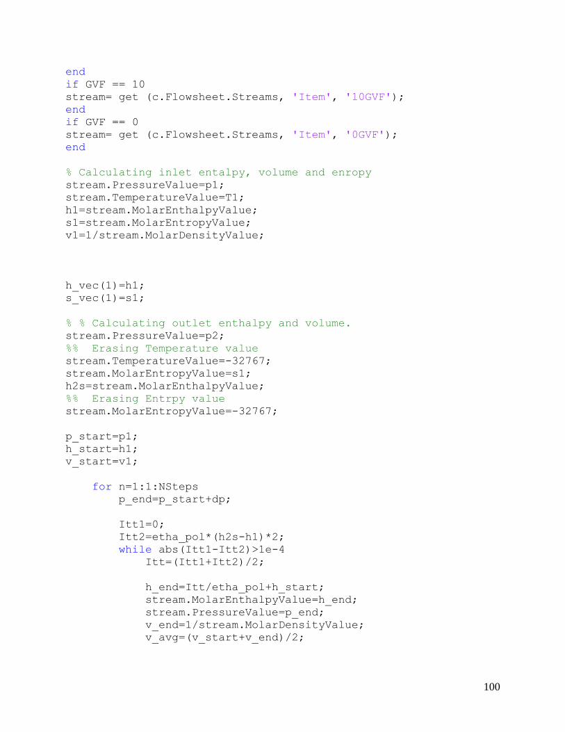
100
end
if GVF == 10
stream= get (c.Flowsheet.Streams, 'Item', '10GVF');
end
if GVF == 0
stream= get (c.Flowsheet.Streams, 'Item', '0GVF');
end
% Calculating inlet entalpy, volume and enropy
stream.PressureValue=p1;
stream.TemperatureValue=T1;
h1=stream.MolarEnthalpyValue;
s1=stream.MolarEntropyValue;
v1=1/stream.MolarDensityValue;
h_vec(1)=h1;
s_vec(1)=s1;
% % Calculating outlet enthalpy and volume.
stream.PressureValue=p2;
%% Erasing Temperature value
stream.TemperatureValue=-32767;
stream.MolarEntropyValue=s1;
h2s=stream.MolarEnthalpyValue;
%% Erasing Entrpy value
stream.MolarEntropyValue=-32767;
p_start=p1;
h_start=h1;
v_start=v1;
for n=1:1:NSteps
p_end=p_start+dp;
Itt1=0;
Itt2=etha_pol*(h2s-h1)*2;
while abs(Itt1-Itt2)>1e-4
Itt=(Itt1+Itt2)/2;
h_end=Itt/etha_pol+h_start;
stream.MolarEnthalpyValue=h_end;
stream.PressureValue=p_end;
v_end=1/stream.MolarDensityValue;
v_avg=(v_start+v_end)/2;

101
reff=v_avg*dp;
if reff>=Itt
Itt1=Itt;
else
Itt2=Itt;
end
end
h_start=h_end;
p_start=p_end;
v_start=v_end;
h_vec(n+1)=h_end;
s_vec(n+1)=stream.molarEntropyValue;
end
stream.MolarEnthalpyValue=h_end;
stream.PressureValue=p_end;
T2=stream.TemperatureValue;
end
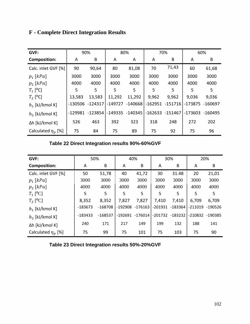
102
F - Complete Direct Integration Results
GVF: 90% 80% 70% 60%
Composition: A B A A A B A B
Calc. inlet GVF [%] 90 90,64 80 81,08 70 71,43 60 61,68
3000 3000 3000 3000 3000 3000 3000 3000
4000 4000 4000 4000 4000 4000 4000 4000
[⁰C] 5 5 5 5 5 5 5 5
[⁰C] 13,583 13,583 11,292 11,292 9,962 9,962 9,036 9,036
[kJ/kmol K] -130506 -124317 -149727 -140668 -162951 -151716 -173875 -160697
[kJ/kmol K] -129981 -123854 -149335 -140345 -162633 -151467 -173603 -160495
∆h [kJ/kmol K] 526 463 392 323 318 248 272 202
Calculated [%] 75 84 75 89 75 92 75 96
Table 22 Direct Integration results 90%-60%GVF
GVF: 50% 40% 30% 20%
Composition: A B A B A B A B
Calc. inlet GVF [%] 50 51,78 40 41,72 30 31.48 20 21,01
3000 3000 3000 3000 3000 3000 3000 3000
4000 4000 4000 4000 4000 4000 4000 4000
[⁰C] 5 5 5 5 5 5 5 5
[⁰C] 8,352 8,352 7,827 7,827 7,410 7,410 6,709 6,709
[kJ/kmol K] -183673 -168708 -192908 -176163 -201931 -183364 -211019 -190526
[kJ/kmol K] -183433 -168537 -192691 -176014 -201732 -183232 -210832 -190385
∆h [kJ/kmol K] 240 171 217 149 199 132 188 141
Calculated [%] 75 99 75 101 75 103 75 90
Table 23 Direct Integration results 50%-20%GVF
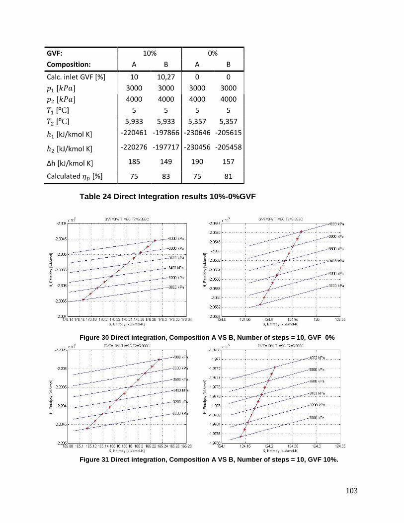
103
GVF: 10% 0%
Composition: A B A B
Calc. inlet GVF [%] 10 10,27 0 0
3000 3000 3000 3000
4000 4000 4000 4000
[⁰C] 5 5 5 5
[⁰C] 5,933 5,933 5,357 5,357
[kJ/kmol K] -220461 -197866 -230646 -205615
[kJ/kmol K] -220276 -197717 -230456 -205458
∆h [kJ/kmol K] 185 149 190 157
Calculated [%] 75 83 75 81
Table 24 Direct Integration results 10%-0%GVF
Figure 30 Direct integration, Composition A VS B, Number of steps = 10, GVF 0%
Figure 31 Direct integration, Composition A VS B, Number of steps = 10, GVF 10%.
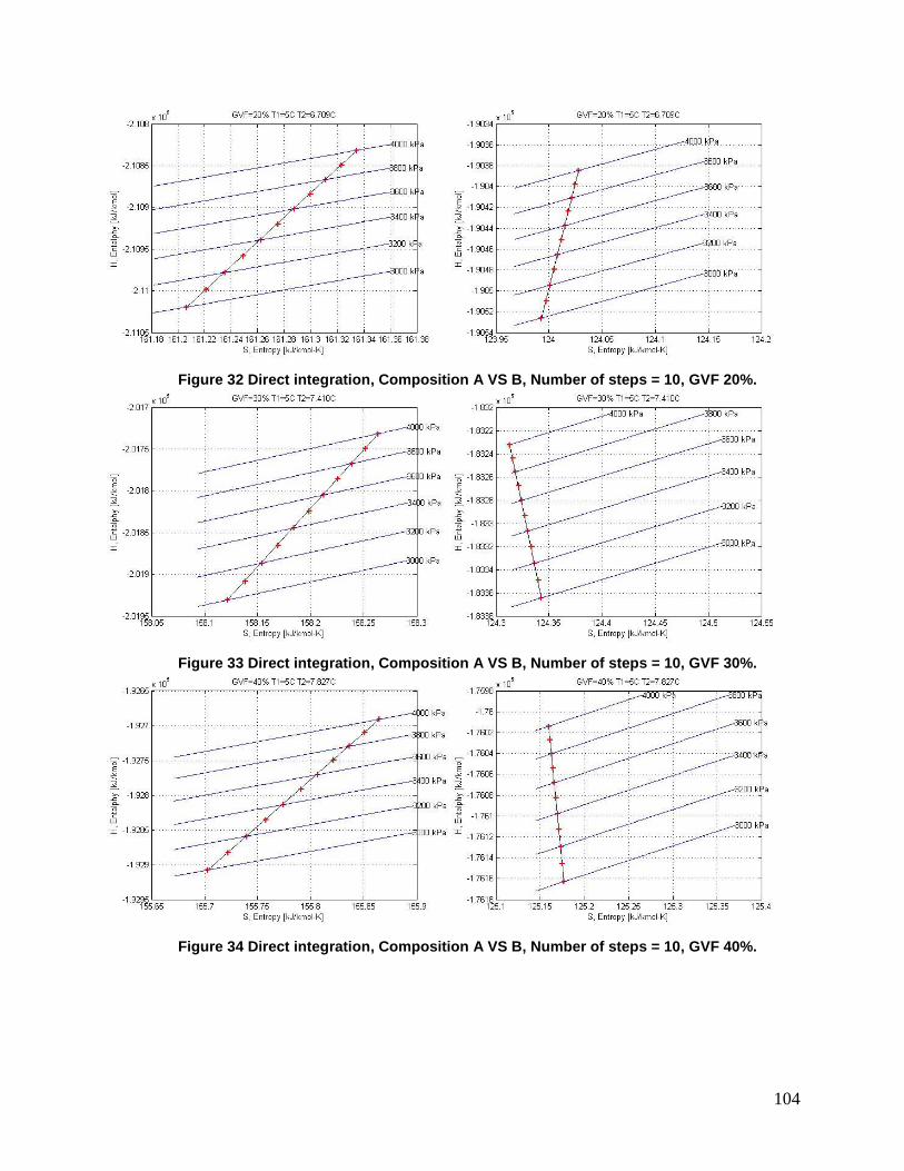
104
Figure 32 Direct integration, Composition A VS B, Number of steps = 10, GVF 20%.
Figure 33 Direct integration, Composition A VS B, Number of steps = 10, GVF 30%.
Figure 34 Direct integration, Composition A VS B, Number of steps = 10, GVF 40%.
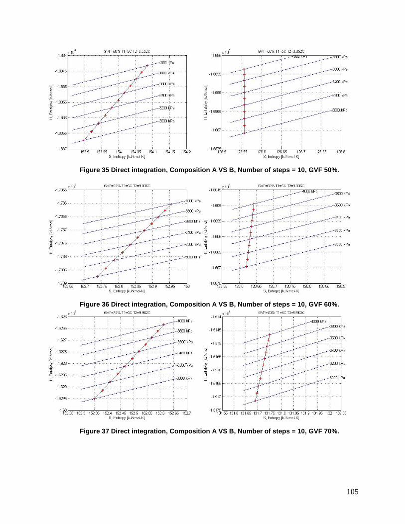
105
Figure 35 Direct integration, Composition A VS B, Number of steps = 10, GVF 50%.
Figure 36 Direct integration, Composition A VS B, Number of steps = 10, GVF 60%.
Figure 37 Direct integration, Composition A VS B, Number of steps = 10, GVF 70%.

106
Figure 38 Direct integration, Composition A VS B, Number of steps = 10, GVF 80%
Figure 39 Direct integration, Composition A VS B, Number of steps = 10, GVF 90%.