multinational time use study user’s guide and documentation · multinational time use study...
TRANSCRIPT

MULTINATIONAL TIME USE STUDY USER’S GUIDE AND DOCUMENTATION Version 2 Feburary 2006
Anne H. Gauthier, Jonathan Gershuny, Kimberly Fisher
With Alyssa Borkosky, Anita Bortnik, Donna Dosman, Cara Fedick, Tyler Frederick, Sally Jones, Tingting Lu, Fiona Lui, Leslie MacRae, Berenice Monna, Monica Pauls, Cori Pawlak, Nuno Torres, and Charlemaigne Victorino
Important: Note that this User Guide and Documentation pertains to Release 2 of the World5.5 dataset and replaces Release 1 (March 2003) and also the first version of Release 2 issued in May 2005. Numerous errors have been corrected in this new Release and new variables have been added.

Table of contents Acknowledgements Disclaimer Introduction Chapter 1: Overview of the MTUS dataset Chapter 2: Codes of activities
Chapter 3: Demographic and socio-economic variables
Chapter 4: Weights in MTUS Chapter 5: The analysis of time-use data Bibliography Appendix: Readme files for each country

Acknowledgements:
The development of the Multinational Time Use Study (MTUS) spanned several decades, involved numerous research assistants, and various sources of funding. The authors of this User's Guide are particularly grateful to our statistical partners without whom MTUS would not have been possible. We especially appreciate their willingness to share the datasets with us and to answer our numerous questions about them.
It would be impossible to list all of them. Among our most recent collaborators, we are grateful to Michael Bittman (Australia), Jens Bonke (Denmark), Koen Breedveld (Netherlands), Françoise Dumontier (France), Manfred Ehling (Germany), Andrew Harvey (Canada), Duncan Ironmonger (Australia), Glenn Moss (South Africa), Iiris Niemi (Finland), Hannu Pääkkönen (Finland), John Robinson (United States), Klas Rydenstam (Sweden), Endre Sik (Hungary), Faye Soupourmas (Australia), Oriel Sullivan (Israel), and Odd Frank Vaage (Norway).
In addition, we are grateful to the following national statistical agencies: the Australian Bureau of Statistics (ABS), the Austrian Central Statistical Office, the French National Institute of Statistics and Economic Studies (INSEE), the German Federal Statistical Office, the Italian National Statistical Institute (ISTAT), Statistics Canada, Statistics Finland, Statistics Norway, Statistical Office of the Republic of Slovenia, Statistics South Africa, Statistics Sweden, and the United Kingdom Office for National Statistics (ONS).
We are also grateful to the following funding agencies which have supported our research program over the years: the Canada Research Chair Program, the Canadian Social Sciences and Humanities Research Council, the Economic and Social Research Council (ESRC) (England), the European Foundation for the Improvement of Living and Working Conditions (EFILWC) (Ireland), the Office for National Statistics (ONS) (UK), the University of Essex (UK), the University of Melbourne (Australia), and The Joseph Rowntree Memorial Trust (UK).
The authors of this User's Guide take full responsibilities for omissions and errors.

Disclaimer: Although we aimed at the highest level of accuracy when preparing this document, errors are possible. Users of the MTUS dataset do so at their own risks! Note also that the User’s Guide thoroughly documents the recoding of the harmonized variables for the Release 2 version of World5.5 datasets. An earlier version of the harmonized dataset is available for a larger number of surveys (World5.0). These additional surveys have not yet been checked for cross-survey consistency. They will be gradually be checked and added to future releases.

1
INTRODUCTION This User’s Guide and Documentation is the companion document to the MTUS dataset. Information on other time use surveys not included in the harmonized version of the dataset, as well as other information on the MTUS project can be found on-line: http://www.timeuse.org/mtus/. This User Guide is publicly available. Access to the data is however restricted and requires authorization from the MTUS board (see: http://www.timeuse.org/mtus/access/). The User’s Guide describes the structure of the MTUS dataset and discusses issues of comparability across surveys. To date, nearly 60 time use surveys have been archived at MTUS. This User’s Guide however pertains to only a subset of these surveys. Future releases of the dataset and User’s Guide will gradually cover all the surveys currently archived at MTUS, in addition to new surveys. A tentative timetable of future releases can be found on the MTUS website at: http://www.timeuse.org/mtus/timetable/. The current version of this User’s Guide covers the following countries and surveys:
Australia 1987, 1992, 1997 Austria 1992 Canada 1971/72, 1981, 1986, 1992, 1998 Denmark 1964 Finland 1979, 1987/88, 1999 France 1998 Germany 1991/92 Italy 1989 The Netherlands 1975, 1980, 1985, 1990, 1995, 2000 Norway 1971, 1981, 1990/91, 2000 Slovenia 2000 South Africa 2000 Sweden 1990/91, 2000 UK 1961, 1974/75, 1983, 1987, 1995, 2000/01 USA 1965/66, 1975/76, 1985, 1992/94, 1998, 2003
Work is currently underway to add the following surveys in a foreseeable future:
Australia 1974 Denmark 1987, 2000 France 1966, 1974, 1985 USA 1995, 1998-2001 (replacing 1998)
2
This User’s Guide describes the surveys and the various harmonized variables. It also discusses the weighting of time use survey as well as the methods of analysis of time use data. It however does not contain survey-specific information regarding the coding of harmonized variables. Such information is instead contained in the survey-specific README documents. Note that this User Guide and Documentation pertains to Release 2 of the World5.5 dataset and replaces Release 1 (March 2003). Numerous errors have been corrected in this new Release and new variables have been added. Note also that the MTUS team has also produced a separate Coding Procedure Document aimed at people involved in the creation of World5.5 files. And while this separate document overlaps to a large extent with the current one, it also contains additional information specific to the recoding of variables and the writing of the corresponding syntax. This document is also available online.
3
CHAPTER 1: OVERVIEW OF THE MTUS DATASET
1.1 Introduction The origins of the Multinational Time Use Study (MTUS) go back to the 1980s following an initiative of Jonathan Gershuny. The idea was to create a cross-nationally harmonized set of time use surveys composed of identically recoded variables. The first version of the MTUS dataset comprised some 20 countries, and has since been regularly expanded. The fifth version, named World5, comprised 35 surveys and was at the basis of the landmark study ‘Changing Times’ by J. Gershuny (2000). The World5 version of the dataset was restricted to the population aged 20 to 59 years old, even though the original version of the surveys covered a wider range of respondents. Following efforts of the MTUS coordinating committee (see: http://www.timeuse.org/mtus/coordinators/), this harmonized version has been expanded to the whole age range of respondents for selected surveys. This User’s Guide describes the harmonized aggregate files for the Release 2 version of World5.5 of nearly 40 surveys. Future releases of this User’s Guide will gradually cover all the surveys in the MTUS archive. The MTUS archive, located at the University of Essex, contains the following files:
Original files: Episode and aggregate files World 5.5: Harmonized aggregate files (all ages) with additional
variables (though where only an older version of a file is available, the data remain in the older MTUS format).
For the benefit of Users, we have also created a mega World5.5 file that merged all World5.5 surveys. Note however that the value labels for the variables EDUCA, INCORIG and EMPINCLM are not included in this mega file (the merging process prevented us from retaining the original value labels). All the other variables are harmonized across surveys and not affected by this merge.
4
1.2 About the format and structure of the datasets The surveys are saved in SPSS format. The harmonized versions of the datasets are aggregate files that indicate the total amount of time spent on various activities during a 24-hour period. In future versions of the harmonized datasets, we plan to add episode (or sequential) data. Each case in the dataset corresponds to one diary day. In surveys having carried out a 1-day diary, there is a direct correspondence between each case and each respondent. However, in the case of multiple-day diaries, each case corresponds to one diary-day and one respondent may therefore be represented by more than one case in the dataset. For example, in a survey having carried out a 2-day diary, each respondent would appear twice in the dataset, i.e. as two separate cases. In most descriptive analyses, MTUS Users are encouraged to use all cases and disregard the fact that the total number of cases (i.e. diaries) correspond to a smaller number of respondents. However, when carrying out analyses based on inferential statistics, MTUS Users should be aware of the non-independence of cases and should use appropriate statistical techniques (this issue is discussed in further details in Chapter 5). MTUS Users should also be aware that in surveys based on 7-day diaries (such as those carried out in the Netherlands), each case represents the average across the 7 days of the week instead of 1 diary day as in the other surveys. This aggregation introduces elements of non-comparability with other surveys, especially regarding the estimation of participation rates. In future versions of the datasets, we hope to revise these datasets and instead provide Users with a version for which each case will correspond to one diary day. While creating the harmonized version of the dataset, we included in the syntax a statement to retain only complete diaries, that is, diaries that added up to 24 hours (1440 minutes). We moreover excluded diaries that included more than 60 minutes of unclassifiable or missing time. The documentation specific to each survey (the README files) includes information on the number of cases excluded by this procedure.
5
1.3 List of surveys included in MTUS
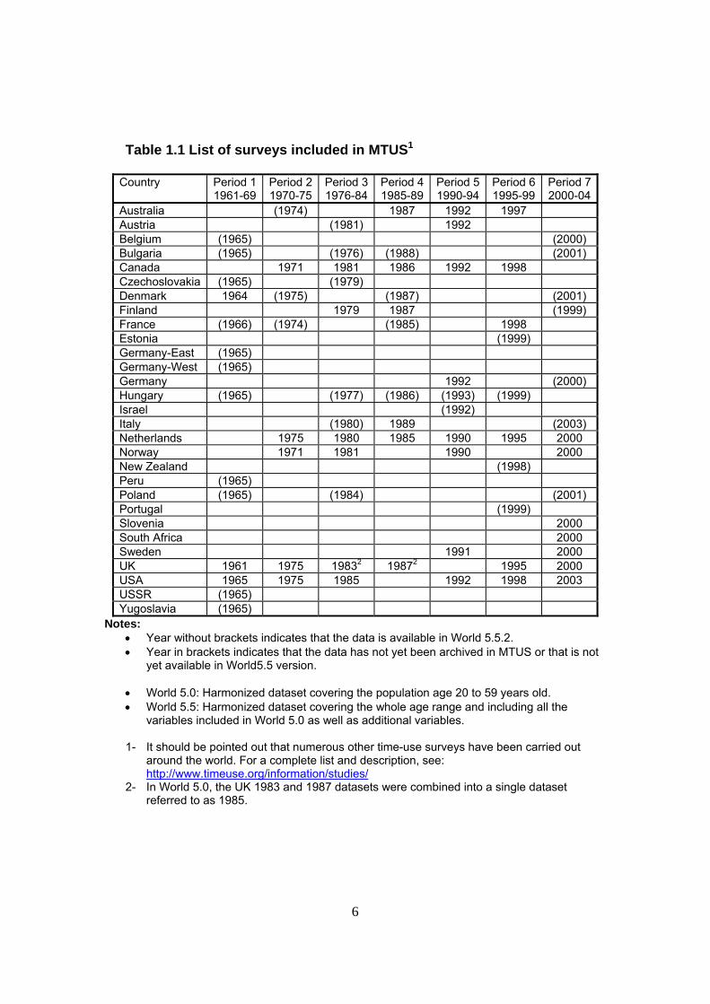
The following table lists all the surveys included in MTUS. The table also lists some of the surveys that we hope to include in the archive in the coming years. For ease of comparison, we distinguish seven time periods. This ‘Period’ is in fact one of the harmonized variables in the dataset. Its cut-off points were chosen in order to make sure that no more than one survey from any given country would be included in each period, and in order to maximise the number of countries included in each period. In Table 1.1, the figures indicated for each country correspond to the actual year when the survey was carried out. Years indicated without (brackets) correspond to surveys for which a
World 5.5 version is available. Years indicated with (brackets) correspond to surveys for which only an
earlier version of World 5.0 is currently available or for which we hope to one day have a version but which is not presently in the data.
In this User’s Guide, we only cover surveys noted without (brackets). As indicated in the introduction, our aim is to eventually cover all the surveys. Note that in several of the surveys, the data collection extended over more than one year (for example from October 1980 to September 1981). In such cases, we usually gave to the variable ‘Survey’, the first year of the data collection (exceptions to this rule are documented in the survey-specific README documents).
6
Table 1.1 List of surveys included in MTUS1
Country Period 1
1961-69 Period 21970-75
Period 31976-84
Period 41985-89
Period 51990-94
Period 6 1995-99
Period 72000-04
Australia (1974) 1987 1992 1997 Austria (1981) 1992 Belgium (1965) (2000) Bulgaria (1965) (1976) (1988) (2001) Canada 1971 1981 1986 1992 1998 Czechoslovakia (1965) (1979) Denmark 1964 (1975) (1987) (2001) Finland 1979 1987 (1999) France (1966) (1974) (1985) 1998 Estonia (1999) Germany-East (1965) Germany-West (1965) Germany 1992 (2000) Hungary (1965) (1977) (1986) (1993) (1999) Israel (1992) Italy (1980) 1989 (2003) Netherlands 1975 1980 1985 1990 1995 2000 Norway 1971 1981 1990 2000 New Zealand (1998) Peru (1965) Poland (1965) (1984) (2001) Portugal (1999) Slovenia 2000 South Africa 2000 Sweden 1991 2000 UK 1961 1975 19832 19872 1995 2000 USA 1965 1975 1985 1992 1998 2003 USSR (1965) Yugoslavia (1965)
Notes: • Year without brackets indicates that the data is available in World 5.5.2. • Year in brackets indicates that the data has not yet been archived in MTUS or that is not
yet available in World5.5 version.
• World 5.0: Harmonized dataset covering the population age 20 to 59 years old. • World 5.5: Harmonized dataset covering the whole age range and including all the
variables included in World 5.0 as well as additional variables.
1- It should be pointed out that numerous other time-use surveys have been carried out around the world. For a complete list and description, see: http://www.timeuse.org/information/studies/
2- In World 5.0, the UK 1983 and 1987 datasets were combined into a single dataset referred to as 1985.

7
1.4 Technical information on the surveys The table below contains key information on the sample size, age of respondents, response rate, etc. for each of the surveys for which a World 5.5 dataset is available. Further information on each survey is included in the country-specific README documents. Table 1.2 Technical information on the time use surveys
Country1 Year Age Sample
Size2 Survey
Period (# months)3
Response rate (%)
Diary (#
days)
Type of diary
Time interval
Household members4
AUS 1987 15+ 1011 2 74.2% 2 On day 15min Yes 1992 15+ 7045 11 82.9% 2 On day 5 min Yes 1997 15+ 7246 8 72.0% 2 On day 5 min Yes OST 1992 10+ 25233 2 47.0% 1 On day 30 min Yes CAN 1971 18-64 2141 8 72.0% 1 On day Free Yes 1981 15+ 2686 3 46.0% 1 On day Free No 1986 15+ 9946 3 78.9% 1 On day Free No 1992 15+ 9815 12 77.0% 1 Recall Free No 1998 15+ 10749 12 77.6% 1 Recall Free No DEN 1964 15+ 4069 2 80.4% 1 Recall 30/15 min In limited cases FIN 1979 10-64 12038 4 81.0% 2 On day 10 min No 1987 15+ 7758 12 74.0% 2 On day 10 min No 1999 10+ 10561 12 52.0% 2 On day 10 min Yes FRA 1985/6 15+ 16047 12 66.9% 1 On day 5 min Yes 1998/9 15+ 15441 12 88.3% 1 On day 10 min Yes GER 1991/2 12+ 7200 4 Quota 2 On day 5 min Yes ITA 1988/9 3+ 38110 12 70.0% 1 On day Free Yes NET 1975 12+ 1309 1 76.0% 7 On day 15 min No 1980 12+ 2730 1 54.0% 7 On day 15 min No 1985 12+ 3263 1 54.0% 7 On day 15 min No 1990 12+ 3158 1 49.0% 7 On day 15 min No 1995 12+ 3227 1 20.0% 7 On day 15 min No 2000 11+ 1813 1 25.0% 7 On day 15 min No NOR 1971/2 16-74 3040 12 58.0% 2 & 3 On day 15 min No 1980/1 16-74 3307 12 65.0% 2 On day 15 min No 1990/1 16-79 3097 12 64.0% 2 On day 15 min No 2000/1 9+ 3211 12 50.0% 2 On day 10 min Yes SLO 2000/1 10+ 4500 12 52.5% 2 On day 10 min Yes RSA 2000 10+ 14553 3 94.0% 1 Recall 10 min Yes SWE 1990/1 20-64 3943 9 75.0% 2 On day 10 min No 2000/01 20-99 3976 12 50% 2 On day 10 min No

8
Country1 Year Age Sample Size2
Survey Period (# months)3
Response rate (%)
Diary (#
days)
Type of diary
Time interval
Household members4
UK 1961 15+ 2363 1 69.8% 7 On day 30 min Yes 1974/5 5+ 3583 4 60.0% 7 On day 30 min Yes 1983/4 14+ 1525 2 51.0% 7 On day 15 min Yes 1987 16+ 3035 1 70.0% 7 On day 15 min Yes 1995 16+ 1875 1 93.0% 1 Recall 15 min No 2000 8+ 11667 12 45.0% 2 On day 10 min Yes USA 1965 18-64 1243 7 74.0% 1 On day Free Yes 1975/76 18+ 2406 3 72.0% 1 On day Free No 1985 12+ 5358 12 55.2% 1 On day
+ recall Free Yes
1992/4 0+ 9386 12 63.0% 1 Recall Free No 1998/20
01 18+ 1700 12 56.0% 1 Recall Free No
2003 15+ 20720 12 57.0% 1 Recall Free No Notes:
1- More countries have carried out time use surveys. A complete list is available at the MTUS web site: http://www.timeuse.org/information/studies/
2- Unless otherwise indicated, the sample size refers to the number of individuals. The actual number of cases is larger in surveys where 2 or 3 diaries were collected.
3- ‘Period’ refers to different collection periods throughout the year. 4- Indicates whether or not more than 1 household member was included in the survey.
Sources: Authors’ tabulation from information contained in Fisher (2000) and various country-specific documents. See the README documents for more information on each survey.
1.5 About the file naming convention We have standardized the way files are named in MTUS. The name of each file distinguishes:
The country (2 or 3-letter code) (see Table 1.3) The year of the survey (4-digit) The version of the archive (Original, World5.0, World5.5) The release number The type of file (extension ‘sav’ for a SPSS data file, and extension
‘sps’ for a SPSS syntax file) For example, Release 2 of the World 5.5 version of Canada 1992 is called ‘Can1992W552.sav’, which should be read as:
Country: Can Year: 1992 Version: W55 (i.e. World5.5) Release: 2 Type: sav

9
Note that in surveys for which the data collection spread over more than 1 year, SURVEY takes the value of the year when the data collection began. For example, Finland 1987/88 is referred to as FIN1987. For exceptions to this rule, see the survey-specific README documents.
Table 1.3: Countries’ code
Country CodeAustralia AUS Austria OST Belgium BEL Canada CAN Czechoslovakia CZE Denmark DEN Finland FIN France FRA Germany GER Germany - East GDR Germany - West FRG Hungary HUN Israel ISR Italy ITA Netherlands NET Norway NOR Peru PER Poland POL Slovenia SLO South Africa RSA Sweden SWEUnited Kingdom UK United States USA Yugoslavia YUG
1.6 Missing value conventions
We use three codes to mark missing values, and a separate fourth convention for weights and identifier variables that are not present. “-7” refers to situations for we can create a variable for this survey, but we
cannot create the variable for this diarist (or diary) as the respondent was not asked for the information on this diary or because the information is not relevant to that respondent (such as the employment status of a spouse for a person who is single and not living with a co-habiting partner). Although the “-
10
7” option potentially applies to all variables, it is mainly used for AGEKID, WORHRS, EMPSP, EMPINCLM.
“-8” refers to situations where we can create the harmonised variable for the study, but no information is recorded for this case (item non-response).
“-9” refers to situations for which the harmonised variable could not be computed for the survey (with exceptions for weights and identifier variables). Note that we use -9 with the time use activity variables to distinguish true 0s (the diarist did not record any time in this activity, though in theory they could have done so) from cases where no time is recorded in the activity because we could not create this time use category for this survey.
There are cases where an identifier variable and where a type of weight is not present or not constructed. In these cases, we use “0” rather than a missing value to indicate that this identifier or weight is not present in the study. IMPORTANT NOTES There are no system missing cases in World5.5 data files. All cases for all variables have either a valid value or a standardised missing value. The World 5.5 data files contain no declared missing values. MTUS users need to declare missing values if they choose to do so before running their analysis. In SPSS, the commands to do so are as follows: Example: Recode AV1 to AV41 (0=-9). execute.

11
CHAPTER 2: CODES OF ACTIVITIES
A first series of cross-nationally comparable surveys was carried out in the 1960s under the direction of Alexander Szalai. The harmonized typology of activities contained 90 different codes (Szalai 1972). Subsequent surveys have used variants of this original typology, providing fewer or more details. In the context of MTUS, a harmonized 41-activity coding was developed in order to reconcile the various typologies. An additional 22-activity typology was also developed to cover surveys that have a more restricted set of activity codes. Information on these harmonized codes of activities appears below. Additional interpretation rules are included in this chapter. Information on how each survey’s original codes of activities were recoded into these harmonized codes may be found in the survey-specific REDAME documents.
2.1 The MTUS 41-activity typology The following 41-activity codes are available in the various harmonized versions of the MTUS dataset. The sum of these activities is equal to 1440 minutes (24 hours). Table 2.1: Harmonized codes of activities (41-activity typology)
41-activity codes
Description
AV1 Time in paid work AV2 Time in paid work at home AV3 Time in paid work, second job AV4 Time in school, classes AV5 Time in travel to/from work AV6 Time cooking, washing up AV7 Time spent doing housework AV8 Time spent doing odd jobs AV9 Time spent gardening AV10 Time spent shopping AV11 Time spent in childcare AV12 Time spent during domestic travel AV13 Time for dressing/toilet AV14 Time spent receiving personal services AV15 Time spent eating meals and snacks

12
AV16 Time spent sleeping AV17 Time spent during travel for leisure AV18 Time spent on excursions AV19 Time spent actively participating in sports AV20 Time spent passively participating in sports AV21 Time spent walking AV22 Time in religious activities AV23 Time doing civic duties AV24 Time at the cinema or theatre AV25 Time at dances or parties AV26 Time at social clubs AV27 Time at pubs AV28 Time at restaurants AV29 Time visiting friends AV30 Time listening to radio AV31 Time watching the television or video AV32 Time listening to records, tapes, cds AV33 Time in study AV34 Time reading books AV35 Time reading papers, magazines AV36 Time relaxing AV37 Time in conversation AV38 Time entertaining friends AV39 Time knitting, sewing, etc AV40 Time in other hobbies or pastimes AV41 Time in unclassifiable activities, or not
recorded Users are advised to be very familiar with the coding of activities in order to avoid misinterpretations of some of the results. The following sections of this chapter draw attention to some of the activities that could have been classified elsewhere under a different classification scheme.

13
2.2 The MTUS 22-activity typology A second set of harmonized codes is also available in the harmonized version of the MTUS dataset. The correspondence between the 41-activity codes and the 22-activity codes appears below. Table 2.2 Harmonized codes of activities (20-activity typology) 22-activity code DESCRIPTION Correspondence with
41-activity codes PAIDETC Time spent in paid work, etc. AV1, AV2, AV3, AV5 HWORK Time spent in routine housework AV7 COOKING Time spent on cooking and food
preparation AV6
EATING Time eating meals and snacks AV15 KIDCARE Time spent on child care AV11 SHOPPING Time spent shopping (all sorts) AV10 DTRAVEL Time spent on domestic related
travel AV12
OTRAVEL Time spent on other non-work travel
AV17, AV18
PERSCARE Time spent on personal care activities
AV13, AV16
EATOUT Time spent eating out AV28 PUBCLUBS Time spent at pubs and clubs AV26, AV27 SPECTAT Time spent as a spectator of an
event AV20, AV22, AV23, AV24, AV25
ASPORTS Time spent in active sports AV19 WALKING Time spent walking AV21 VISITS Time spent visiting or entertaining
friends AV29, AV38
TVRAD Time spent watching television/listening to radio
AV30, AV31, AV32
READING Time reading books, papers, or magazines
AV33, AV34, AV35
CHATSETC Time spent talking or relaxing AV36, AV37 ODDJOBS Time spent in non-routine
domestic work AV8, AV9
HOBBIES Other at home leisure AV39, AV40 MEDICAL Medically related personal care AV14 EDUC Time spent in education AV4

14
2.3 Overall degree of cross-survey comparability The extent to which it was possible to create the AV harmonized codes is partly a function of the number of codes originally used in each survey. The table below provides further information on these codes. Table 2.3 Information on the codes of activities used in each survey (prior to harmonization) Country Year Number of
codes Range
Australia 1987 57 010 to 980 1992 281 000 to 999 1997 215 0 to 999 Austria 1992 197 111 to 900 Canada 1971 100 00 to 99 1981 272 001 to 990 1986 99 01 to 99 1992 167 001 to 990 1998 178 001 to 999 Denmark 1964 22 1 to 41 Finland 1979 100 1 to 99 1987 100 1 to 100 2000 265 0 to 9990 France 1985 200 1 to 199 1999 145 111 to 911 Germany 1992 231 11 to 999 Italy 1989 150 1001 to 6009 Netherlands 1975 – 1995* 354 000 to 999 2000 354 000 to 9999 Norway 1971 97 1 to 99 1981 97 1 to 99 1990 123 700 to 1310 2000 265 0 to 9990 Slovenia 2000 265 0 to 9990 South Africa 2000 99 010 to 990 Sweden 1991 108 110 to 6121 Sweden 2000 150 0 to 999 UK 1961 106 001 to 193 1975 73 1 to 99 1983 185 101 to 9999 1987 193 101 to 9999 1995 31 1 to 31

15
Country Year Number of codes
Range
2000 268 0 to 9990 USA 1965 100 00 to 99 1975 175 000 to 999 1985 88 0 to 99 1992 91 1 to 99 1998 94 1 to 99 2003 91/564 1 to 98/3 tiers Notes:
* Based on the merged 1975 to 1995 file provided by the Netherlands. This merged file contains identical codes across the 5 surveys. The codes for each individual survey may have differed prior to this harmonization.
2.4 Details of the codes of activities We report below details of the 41-activity codes as well as drawing attention to specific interpretative rules that were adopted by the MTUS team. AV1: Paid Work MTUS 4-Digit Codes: 0101 Normal work 0102 Unscheduled break at work 0103 Scheduled break at work (eg meal) 0104 Other work-related activities Notes: Any activity done during work hours, but not related to work (i.e.
shopping, going to doctor/dentist) should be coded in their respective categories (i.e. shopping, receiving personal services).
Meal breaks at work or during work hours are to be coded as AV1. Courses/studies taken for work during work hours should be coded
as AV1. Work-related courses taken in free time should be coded as AV4.
Farming as the main economic activity should be coded as AV1. Unpaid help to another business/farm should be coded as AV8.
Unpaid work for family business/farm should be coded as AV3. Any unpaid work at home (related to main job) or conversations
about work but not during work hours should be coded as AV1. General work-related variables to be coded as AV1 (i.e. sundry
work-related activities, “other” work-related activities). AV2: Paid Work At Home MTUS 4-Digit Codes: 0201 Childminding 0202 Running a catalogue 0203 Job seeking paperwork at home

16
0204 (Other) Job search activities 0206 Other home-working (non-computer) 0207 Other home-working (computer) 0208 Work “brought home” (non-computer) 0209 Work “brought home” (computer) Notes: Any code or code related to “unemployment benefits” or “welfare”
should be coded as AV2. “Childminding” implies paid child minding.
AV3: Second Job MTUS 4-Digit Codes: 0301 Second, third etc. job (for money) 0302 Other informal economic activity Notes: Any activity (other than the main occupation) done for sale/exchange
should be coded here (i.e. hobbies, crafts for sale). Any variable implying “help to family business” (paid or unpaid)
should be coded here. AV4: School/Classes MTUS 4-Digit Codes: 0401 Educational activities 0402 Lunch break at education establishment 0403 Student at educational establishment 0404 Other educational activities 0405 Night and privately tutored classes for hobbies Notes: Include codes related to work-related courses done in free time
Include breaks and waiting at school/educational establishment AV5: Travel to/from Work MTUS 4-Digit Codes: 0501 Job seeking activities outside home 0502 Travel to/from work 0503 Education travel 0504 Job search – travel 0505 Other work-related travel Notes: Also includes travel during or for work/school AV6: Cooking/Washing Up MTUS 4-Digit Codes: 0601 Food preparation 0602 Baking, freezing foods, making jams, pickles, preserves, drying
herbs 0603 Washing up, putting away dishes 0604 Making a cup of tea, coffee, etc. 0605 Set table Notes: None AV7: Housework MTUS 4-Digit Codes: 0701 Washing clothes, hanging washing out to dry, bringing it in

17
0702 Ironing clothes 0703 Making, changing beds 0704 Dusting, hovering, vacuum cleaning, general tidying 0705 Outdoor cleaning 0706 Other manual domestic work 0707 Housework elsewhere unspecified 0708 Putting shopping away Notes: Include all “sundry” or “other” house/domestic work variables AV8: Odd Jobs MTUS 4-Digit Codes: 0801 Repair, upkeep of clothes 0802 Heat and water supply upkeep 0803 DIY, decorating, household repairs 0804 Vehicle maintenance, car washing, etc. 0805 Home paperwork (not computer) 0806 Pet care, care of houseplants 0807 (Other) tasks in and around the home, unspecified 0808 Tasks – unspecified 0809 Feeding and food preparation for dependant adults 0810 Washing, toilet needs of dependant adults 0811 Shopping for others 0812 Fetching/carrying for other 0813 Other care of adults 0814 Doing housework for someone else (unpaid) 0815 Care of adults (unspecified) 0816 Service for animals (eg animals to vet) 0817 Fetching, picking up, dropping off 0818 Home paperwork on computer Notes: Include helping/caring for sick/disabled adults (excludes
“volunteering” – see AV23). Include any general care of family (i.e. Italy 1989: AV2411 – “Other
family care activities”). Include obtaining medical care for household adults; also include
self administered medical care and medical care administered to (by respondent) other household adults.
Include unpaid help to others (i.e. house cleaning; farm help; assistance in correspondence, transportation, etc)
Include variables such as “dressmaking” or “making clothes” when they are grouped with other “domestic work” variables in the original dataset. This would imply that they are not leisure activities.
AV9: Gardening MTUS 4-Digit Codes: 0901 Gardening Notes: Include any original variables which combine “gardening” and
“animal care” (i.e. Canada,1971: PRIME11 – “Gardening, animal care”)
AV10: Shopping MTUS 4-Digit Codes: 1001 Everyday shopping, shopping unspecified 1002 Shopping for durable goods
18
1003 Services for upkeep of possessions 1004 Money services 1005 Attending jumble sales, bazaars, etc. 1006 Video rental or return 1007 Other service organizations or use (e.g. travel agent) Notes: Include all activities where a “maintenance service” is used (i.e.
filling up car at the gas station, taking clothes to the cleaners or laundry, etc)
Include all activities labelled “other” or “uncodeable” services. Include “errands” and “running errands”)
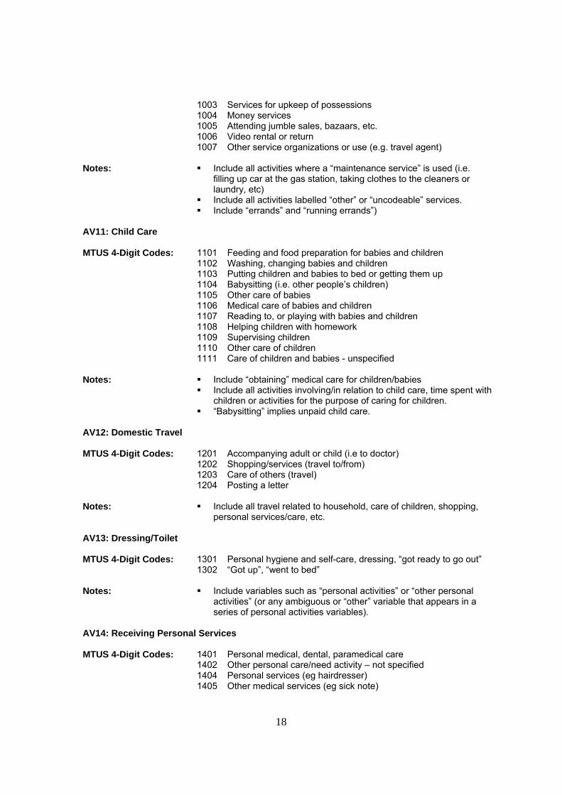
AV11: Child Care MTUS 4-Digit Codes: 1101 Feeding and food preparation for babies and children 1102 Washing, changing babies and children 1103 Putting children and babies to bed or getting them up 1104 Babysitting (i.e. other people’s children) 1105 Other care of babies 1106 Medical care of babies and children 1107 Reading to, or playing with babies and children 1108 Helping children with homework 1109 Supervising children 1110 Other care of children 1111 Care of children and babies - unspecified Notes: Include “obtaining” medical care for children/babies
Include all activities involving/in relation to child care, time spent with children or activities for the purpose of caring for children.
“Babysitting” implies unpaid child care. AV12: Domestic Travel MTUS 4-Digit Codes: 1201 Accompanying adult or child (i.e to doctor) 1202 Shopping/services (travel to/from) 1203 Care of others (travel) 1204 Posting a letter Notes: Include all travel related to household, care of children, shopping,
personal services/care, etc. AV13: Dressing/Toilet MTUS 4-Digit Codes: 1301 Personal hygiene and self-care, dressing, “got ready to go out” 1302 “Got up”, “went to bed” Notes: Include variables such as “personal activities” or “other personal
activities” (or any ambiguous or “other” variable that appears in a series of personal activities variables).
AV14: Receiving Personal Services MTUS 4-Digit Codes: 1401 Personal medical, dental, paramedical care 1402 Other personal care/need activity – not specified 1404 Personal services (eg hairdresser) 1405 Other medical services (eg sick note)
19
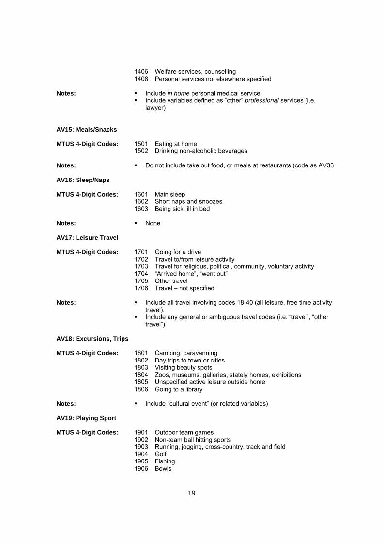
1406 Welfare services, counselling 1408 Personal services not elsewhere specified Notes: Include in home personal medical service
Include variables defined as “other” professional services (i.e. lawyer)
AV15: Meals/Snacks MTUS 4-Digit Codes: 1501 Eating at home 1502 Drinking non-alcoholic beverages Notes: Do not include take out food, or meals at restaurants (code as AV33 AV16: Sleep/Naps MTUS 4-Digit Codes: 1601 Main sleep 1602 Short naps and snoozes 1603 Being sick, ill in bed Notes: None AV17: Leisure Travel MTUS 4-Digit Codes: 1701 Going for a drive 1702 Travel to/from leisure activity 1703 Travel for religious, political, community, voluntary activity 1704 “Arrived home”, “went out” 1705 Other travel 1706 Travel – not specified Notes: Include all travel involving codes 18-40 (all leisure, free time activity
travel). Include any general or ambiguous travel codes (i.e. “travel”, “other
travel”). AV18: Excursions, Trips MTUS 4-Digit Codes: 1801 Camping, caravanning 1802 Day trips to town or cities 1803 Visiting beauty spots 1804 Zoos, museums, galleries, stately homes, exhibitions 1805 Unspecified active leisure outside home 1806 Going to a library Notes: Include “cultural event” (or related variables) AV19: Playing Sport MTUS 4-Digit Codes: 1901 Outdoor team games 1902 Non-team ball hitting sports 1903 Running, jogging, cross-country, track and field 1904 Golf 1905 Fishing 1906 Bowls
20
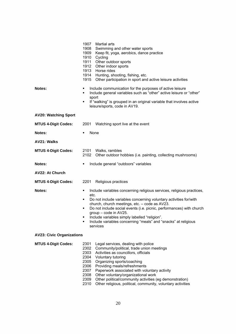
1907 Martial arts 1908 Swimming and other water sports 1909 Keep fit, yoga, aerobics, dance practice 1910 Cycling 1911 Other outdoor sports 1912 Other indoor sports 1913 Horse rides 1914 Hunting, shooting, fishing, etc. 1915 Other participation in sport and active leisure activities Notes: Include communication for the purposes of active leisure
Include general variables such as “other” active leisure or “other” sport
If “walking” is grouped in an original variable that involves active leisure/sports, code in AV19.
AV20: Watching Sport MTUS 4-Digit Codes: 2001 Watching sport live at the event Notes: None AV21: Walks MTUS 4-Digit Codes: 2101 Walks, rambles 2102 Other outdoor hobbies (i.e. painting, collecting mushrooms) Notes: Include general “outdoors” variables AV22: At Church MTUS 4-Digit Codes: 2201 Religious practices Notes: Include variables concerning religious services, religious practices,
etc. Do not include variables concerning voluntary activities for/with
church, church meetings, etc. – code as AV23. Do not include social events (i.e. picnic, performances) with church
group – code in AV25. Include variables simply labelled “religion”. Include variables concerning “meals” and “snacks” at religious
services AV23: Civic Organizations MTUS 4-Digit Codes: 2301 Legal services, dealing with police 2302 Community/political, trade union meetings 2303 Activities as councillors, officials 2304 Voluntary tutoring 2305 Organizing sports/coaching 2306 Providing meals/refreshments 2307 Paperwork associated with voluntary activity 2308 Other voluntary/organizational work 2309 Other political/community activities (eg demonstration) 2310 Other religious, political, community, voluntary activities

21
Notes: Include variables concerning “meetings” (i.e. “church meeting”) AV24: Cinema/Theatre MTUS 4-Digit Codes: 2401 Watching films at the cinema (including other public viewing of
recorded material) 2402 Going to theatre 2403 Other live entertainment (i.e. concert, opera) 2404 Pop concert Notes: None AV25: Dance/Party etc. MTUS 4-Digit Codes: 2501 At a party/dance 2502 Meeting friends, relatives outside respective homes 2503 Gambling (i.e. at betting shop, casino 2504 Driving lessons 2505 Other – leisure and entertainment activities out of home 2506 Leisure and entertainment – not specified 2507 “Went dancing” (i.e. disco or dance hall) 2508 Scouts/Guides etc. Notes: Include variables concerning weddings, family gatherings, religious
performances, etc. Include general out of home “social” variables (i.e. “social away”,
“other social activities”). Include general entertainment variables (i.e. “other entertainment”) The 4-digit MTUS criteria groups “Scouts/Guides” as “Dance/Party”.
However, the literature suggests that Scouts/Guides are a form of social capital and social involvement, which implies that it should ultimately be coded as AV23.
AV26: Social Clubs MTUS 4-Digit Codes: 2601 At a social or night club Notes: None AV27: Pubs MTUS 4-Digit Codes: 2701 At the pub Notes: Include variables such as “at a bar” or “drinking at the bar”. AV28: Restaurants MTUS 4-Digit Codes: 2801 Eating out at restaurants, cafes 2802 Eating out at a fast food or takeaway 2803 Eating out not specified 2804 Eating meal at pub (not snack) Notes: None AV29: Visiting Friends
22
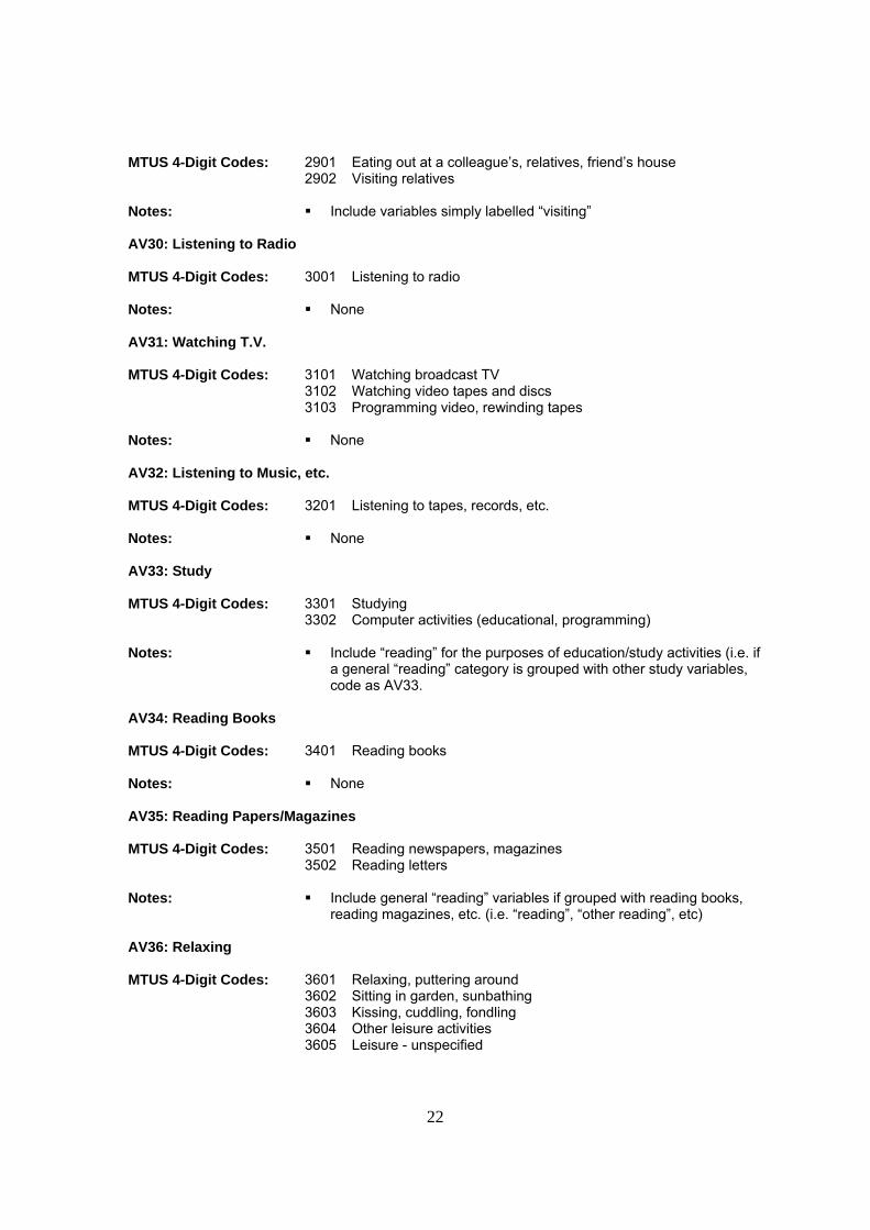
MTUS 4-Digit Codes: 2901 Eating out at a colleague’s, relatives, friend’s house 2902 Visiting relatives Notes: Include variables simply labelled “visiting” AV30: Listening to Radio MTUS 4-Digit Codes: 3001 Listening to radio Notes: None AV31: Watching T.V. MTUS 4-Digit Codes: 3101 Watching broadcast TV 3102 Watching video tapes and discs 3103 Programming video, rewinding tapes Notes: None AV32: Listening to Music, etc. MTUS 4-Digit Codes: 3201 Listening to tapes, records, etc. Notes: None AV33: Study MTUS 4-Digit Codes: 3301 Studying 3302 Computer activities (educational, programming) Notes: Include “reading” for the purposes of education/study activities (i.e. if
a general “reading” category is grouped with other study variables, code as AV33.
AV34: Reading Books MTUS 4-Digit Codes: 3401 Reading books Notes: None AV35: Reading Papers/Magazines MTUS 4-Digit Codes: 3501 Reading newspapers, magazines 3502 Reading letters Notes: Include general “reading” variables if grouped with reading books,
reading magazines, etc. (i.e. “reading”, “other reading”, etc) AV36: Relaxing MTUS 4-Digit Codes: 3601 Relaxing, puttering around 3602 Sitting in garden, sunbathing 3603 Kissing, cuddling, fondling 3604 Other leisure activities 3605 Leisure - unspecified

23
Notes: Include general “passive leisure” variables if grouped with passive leisure variables in original list (i.e. “other passive leisure”, “doing nothing”, “other leisure”, etc)
AV37: Conversation MTUS 4-Digit Codes: 3701 Talking, chatting, arguing, discussing 3702 Telephoning Notes: Include “tantrums”.
Implies general “leisure” conversations. AV38: Entertaining Friends MTUS 4-Digit Codes: 3801 Entertaining at home 3802 Alcohol, tobacco (smoking) and drugs consumption Notes: None AV39: Knitting/Sewing MTUS 4-Digit Codes: 3901 Knitting, sewing, dressmaking Notes: Include only related variables that are part of leisure (i.e. grouped
with other leisure variables); if knitting, sewing, or dressmaking is grouped with “domestic work” types of variables, code as AV8.
AV40: Pastimes/Hobbies MTUS 4-Digit Codes: 4001 Home-brewing, wine making 4002 Watching home movies, slides 4003 “Playing” 4004 Playing video/computer games 4005 Playing games, cards 4006 Artistic and music activities 4007 Hobbies, collections not shown elsewhere 4008 Writing – longhand or typewritten (default) 4009 Writing on word processor 4010 Filling in time budget diary Notes: Include ambiguous computer use variables (i.e. “other computer
use”) AV41: Unknown Activity MTUS 4-Digit Codes: 9999 Entry missing or undecipherable Notes: None

24
CHAPTER 3: DEMOGRAPHIC AND SOCIO-ECONOMIC VARIABLES
In addition to the time-use variables, the MTUS datasets contain a set of harmonized demographic and socio-economic variables. Several of the original datasets contain a larger number of such variables. In the context of MTUS, priority had to be given to variables that were available in all (or most of) the datasets. The list of these variables appears below, while details on how each of these variables was constructed may be found in the survey-specific documentation (the README documents).
3.1 LIST OF VARIABLES Demographic and socio-economic variables included in World 5.5
COUNTRY: Country where the study was conducted PERIOD: Time survey period SURVEY: Survey year SWAVE: Longitudinal study survey marker MSAMP: Multiple samples using same diary instrument ID: Case Identifier PERSID: Person level identifier HLDID: Household identifier DAY: Day of interview MONTH: Month the diary was kept YEAR: Year diary kept DIARY: Diary day SEX: Sex AGE2: Age AGEGR5Y: Five-year age groups CIVSTAT: Civic status COHAB: Respondent is cohabiting FAMSTAT: Individual level family status CPHOME: Unmarried child living in parental home HHTYPE: Household type SINGPAR: Whether diarist is a single parent HHLDSIZE: Number of people in household NCHILD: Number of children under 18 in household AGEKID: Age of the youngest child in household RELREFP: Relation to household reference person
25
EMPSTAT3: New employment status EMP: In paid work UNEMP: Unemployed STUDENT: Student status RETIRED: Retirement status EMPSP: Employment status of the spouse/partner WORKHRS: Hours of paid work last week including overtime INCORIG: Original household income INCOME: Total household income - grouped EMPINCLM: Original monthly income from employment or self-
employment EDUCA: Educational level - original study code EDTRY: Harmonised level of education DISAB: Diarist has a disability or long-term limiting health condition URBAN: Urban or rural household
Note that a series of weights are also included. They are described in Chapter 4.
3.2 CODING OF THE DEMOGRAPHIC AND SOCIO-ECONOMIC VARIABLES
Information is given below on the coding of each demographic and socio-economic variable. Information on how the variables were originally coded in the surveys and how they were recoded in these harmonized variables may be found in the survey-specific documentation (the README documents).
The harmonised background variables cluster into the following sets:
- General information about the surveys and cases - Basic demographic information - Household structure, presence of children, and marital status - Employment status, income, and education - Other harmonised information
Note that the actual order of the variables in World5.5 varies from the one presented here.
General information about the surveys and cases
• COUNTRY • PERIOD • SURVEY • ID • PERSID

26
• HLDID • DAY • MONTH • YEAR • DIARY
COUNTRY: Country where the study was conducted This variable records the country where the survey was carried out. Note that there are separate codes for West Germany, East Germany, and reunified Germany.
Value Label Value Label 1 Canada 18 Italy 2 Denmark 19 Australia 3 France 20 Israel 4 Netherlands 21 Sweden 5 Norway 22 Germany 6 UK 23 Austria 7 USA 24 South Africa 8 Hungary 25 Brazil 9 West Germany 26 Estonia 10 Poland 27 India 11 Belgium 28 Japan 12 Bulgaria 29 Korea (South) 13 Czechoslovakia 30 Mexico 14 East Germany 31 New Zealand 15 Peru 32 Portugal 16 Yugoslavia 33 Romania 17 Finland 34 Slovenia
PERIOD: Time survey period This variable records the period during which the survey was carried out. The values range from 1961-69 (value ‘1’) to 2000-04 (value ‘7’). Precise information on when the survey was carried out is recorded in the variable ‘Survey’. Note that the length of each period is not equal. Cut-off points were chosen to maximise the number of countries in each period and to ensure that there was only 1 survey per period for any specific country. In cases for which multiple surveys were available for a country during a specific period, only one of these surveys has been included in the MTUS dataset.

27
Value Label 1 1961 - 1969 2 1970 - 1975 3 1976 - 1984 4 1985 - 1989 5 1990 - 1994 6 1995 - 1999 7 2000 - 2004 8 2005 – 2009 9 2010 – 2014
SURVEY: Year the survey began This variable records the year during which the survey was carried out. Note that in an earlier version of the harmonised dataset, the survey year was recorded using a 2-digit code (e.g. 66 instead of 1966). We now use 4-digit codes. Note that the data collection in some surveys spanned more than one year. In such cases, the variable SURVEY takes the value of the beginning year (with exceptions described in the relevant README documents).
SWAVE: Longitudinal study wave marker This variable is relevant only for surveys that are longitudinal.
Value Label 0 Not longitudinal1 Wave 1 2 Wave 2 3 Wave 3 4 Wave 4
Note that in the case of Denmark 1987/2001 (with multiple samples), the code ‘1’ indicates a longitudinal case, while the code ‘0’ indicates that that it is not a longitudinal case.
MSAMP: Multiple samples using the same diary instrument
Value Label

28
0 One sample 1 Szalai USA 1965 sample 2 National USA 1965 sample3 Original NHAPS 4 1995 NHAPS supplement
ID: Case identifier This variable records the diary case ID. This variable is not harmonised across surveys. In most surveys, we kept the original ID assigned by the institution having carried out the survey. In some surveys, we computed values from various survey and demographic characteristics of the respondent in order to obtain one unique ID per case. Note that in multiple-day diaries, the ID (being a case identifier) takes a different value than PERSID. In contrast, in one-day diaries, PERSID = ID.
PERSID: Person level identifier This variable records the respondents’ identifier.
HLDID: Household identifier This variable uniquely identifies households for those studies where more than one household member completed a diary. For surveys in which only one person per household completed a diary and no household identifier is included in the original data, HLDID=0. For surveys in which only one person per household completed a diary but a household identifier is included, HLDID takes the original value for the corresponding variable.
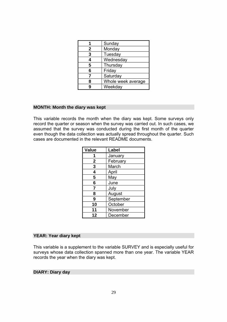
DAY: Day of interview This variable records the day of the week when the diary was kept. Note that in the current version of World5.5, we still have some surveys that appear as 7-day averages rather than as single-day cases. We intend to change the data to individual day data in future versions of the MTUS.
Value Label
29
1 Sunday 2 Monday 3 Tuesday 4 Wednesday 5 Thursday 6 Friday 7 Saturday 8 Whole week average 9 Weekday
MONTH: Month the diary was kept
This variable records the month when the diary was kept. Some surveys only record the quarter or season when the survey was carried out. In such cases, we assumed that the survey was conducted during the first month of the quarter even though the data collection was actually spread throughout the quarter. Such cases are documented in the relevant README documents.
Value Label 1 January 2 February 3 March 4 April 5 May 6 June 7 July 8 August 9 September 10 October 11 November 12 December
YEAR: Year diary kept
This variable is a supplement to the variable SURVEY and is especially useful for surveys whose data collection spanned more than one year. The variable YEAR records the year when the diary was kept.
DIARY: Diary day

30
This variable records the number of the diary (e.g. 1st completed diary, 2nd completed, 3rd completed). In the case of single-day diaries, this variable takes the value 1. In the case of multiple-day diaries, this variable can take the value 1, 2 or 3.
Value Label 1 First diary day 2 Second diary day 3 Third diary day 4 Fourth diary day 5 Fifth diary day 6 Sixth diary day 7 Seventh diary day 8 Weekly average
Basic demographic information • SEX • AGE2 • AGEGR5Y • CIVSTAT • COHAB
SEX: Sex
Value Label 1 Man 2 Woman
AGE2: Age This variable records the age of respondents (up to 3 digits). For surveys in which age was recorded in categories, we recoded age into a continuous variable by assigning the mid-point of each age group (e.g. 17 for age group 15-19). When surveys only included the year of birth of respondents, we computed AGE2 by subtracting the year of birth from the year of the survey.

31
AGEGR5Y: Five-year age groups This variable records the age of respondent in 5-year age group categories. This variable is derived from AGE2.
Value Label 1 0-4 2 5-9 3 10-14 4 15-19 5 20-24 6 25-29 7 30-34 8 35-39 9 40-44 10 45-49 11 50-54 12 55-59 13 60-64 14 65-69 15 70-74 16 75-79 17 80+
CIVSTAT: Civic status This variable records the diarist’s marital status. This variable is highly comparable across countries apart from the fact that most of the earlier surveys did not include a separate category for ‘cohabiting’ or ‘common-law’. It is not possible to know how people living in such unions declared their marital status. They could have declared themselves as being married or as being single therefore introducing some elements of non-comparability.
Value Label 1 Married or cohabiting 2 Not living with a spouse/partner

32
COHAB: Respondent is cohabiting This variable indicates whether or not the diarist is cohabiting with (but not legally married to) a partner.
Value Label 0 Not cohabiting 1 Cohabiting
Household structure and presence of children
• FAMSTAT • CPHOME • HHTYPE • SINGPAR • HHLDSIZE • NCHILD • AGEKID • RELREFP
FAMSTAT: Individual level family status This variable is an individual characteristic, which means that not every member of a household would be coded the same way (in the case of multi-member surveys). It records the presence of children in the household, but does not always allow us to identify whether the children were the diarist’s own children, children of the spouse/partner, or children of another household member.
Value Label 0 Adult aged 18 to 39 with no co-resident children <18 1 Adult 18+ living with 1+ co-resident children aged <5 2 Adult 18+ living with 1+ co-resident children 5-17, none <5 3 Adult aged 40+ with no co-resident children <18 4 Respondent aged <18 and living with parent(s)/guardian(s) 5 Respondent aged <18, living arrangement other or unknown
This variable is highly comparable across countries, though the information about the age of children varies by survey. Discrepancies are documented with the variable AGEKID. Note that it was not possible to identify category ‘4’ for some surveys.

33
CPHOME: Unmarried child living in parental home This variable indicates whether or not diarists who are not married or cohabiting live with their parents, regardless of the diarists’ age. This variable could not be computed in a large number of surveys.
Value Label 0 Not a child in parental home 1 Child in parental home
HHTYPE: Household type This variable records the type of household in which the diarist lived at the time of the survey. Note that the value ‘1’ (one person household) includes never-married, separated, divorced, and widowed people living alone. This variable was computed from a household type variable when available, and from a combination of marital status and household size when no household type classification was available in the original survey.
Value Label 1 One person household 2 married couple alone 3 married couple + others 4 other household types
In some surveys, we cannot identify cohabiting couples, and these people may be miscoded as HHTYPE =4.
In contrast to FAMSTAT, this variable is a household characteristic and all household members should be coded the same way.
SINGPAR: Whether diarist is a single parent This variable records whether or not the diarist is a single-parent.
Value Label0 No 1 Yes

34
HHLDSIZE: Number of people in household This variable records the total number of household members. This variable is highly comparable across surveys. In some surveys, the size of large households is capped, with the value ‘n’ meaning ‘n or more members’. Such cases are documented in the README documents.
NCHILD: Number of children under 18 in household This variable records the total number of children aged under 18 in the household. The children are not necessarily the diarist’s own children. They can be a spouse/partner’s children, children of another household member, younger siblings, or the respondent him/herself if he/she is under 18 years old. Although this variable is highly comparable across countries, it is affected by four problems. First, in numerous surveys, the original variable used to create NCHILD referred to the number of children under 15 instead of 18. Second, in some surveys the original variables used to create AGEKID and NCHILD referred to children of different age groups (for example under 15 for NCHILD, and 13-17 for AGEKID). Third, in most surveys NCHILD refers to the number of children residing in the household, while in others it refers to the number of children of the diarist (without specifying whether or not they reside in the diarist’s household). Finally, in some surveys the original question about the number of children was only asked to diarists who were over 18 years old therefore leaving diarists less than 18 years old with a missing value. In all these cases, we made adjustments and corrections when possible. Users are asked to consult the README documents for more detailed explanations.
AGEKID: Age of youngest child in household This variable records information on the age of the youngest child in the household. If there are no children under 18 in the household, this variable takes the value -7 (even if the original survey gives a valid value for such cases).
Value Label 1 Youngest child between 0-4 2 Youngest child between 5-12 3 Youngest child between 13-17
This variable is highly comparable across surveys. However, the cut-off point for the age of the child varies across surveys. Also, in some surveys the data

35
correspond to the diarist’s children rather than children residing in the diarist’s household.
RELREFP: Relation to household reference person This variable indicates the relationship of the diarist to the household reference person. In the MTUS, the reference person may be any one of the following:
- either spouse in any married couple living in the dwelling; - either partner in a common-law relationship; - the parent, where one parent only lives with his or her never-married son(s) or daughter(s) of any age; - the designated head of household in some older studies.
This variable tends to be collected mainly in surveys in which more than one household member was surveyed.
Value Label 1 Person 1 2 Spouse/ Common-law partner3 Child 4 Parent 5 Sibling 6 Son/Daughter-in-law 7 Father/Mother-in-law 8 Brother/Sister-in-law 9 Other Relative 10 Not related
Employment status, income, and education • EMPSTAT3 • EMP • UNEMP • STUDENT • RETIRED • EMPSP • WORKHRS • INCORIG • INCOME • EMPINCLM • EDUCA • EDTRY
36
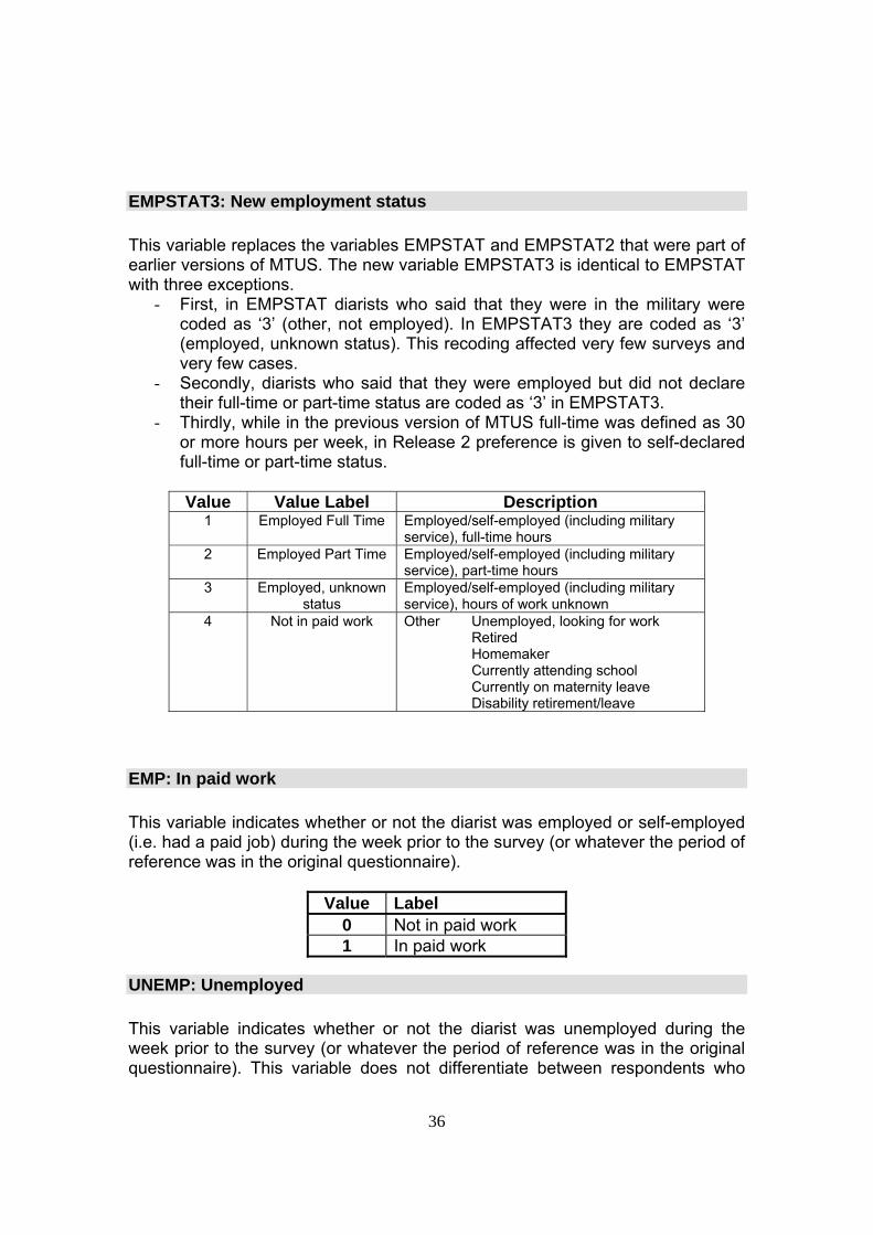
EMPSTAT3: New employment status This variable replaces the variables EMPSTAT and EMPSTAT2 that were part of earlier versions of MTUS. The new variable EMPSTAT3 is identical to EMPSTAT with three exceptions.
- First, in EMPSTAT diarists who said that they were in the military were coded as ‘3’ (other, not employed). In EMPSTAT3 they are coded as ‘3’ (employed, unknown status). This recoding affected very few surveys and very few cases.
- Secondly, diarists who said that they were employed but did not declare their full-time or part-time status are coded as ‘3’ in EMPSTAT3.
- Thirdly, while in the previous version of MTUS full-time was defined as 30 or more hours per week, in Release 2 preference is given to self-declared full-time or part-time status.
Value Value Label Description
1 Employed Full Time Employed/self-employed (including military service), full-time hours
2 Employed Part Time Employed/self-employed (including military service), part-time hours
3 Employed, unknown status
Employed/self-employed (including military service), hours of work unknown
4 Not in paid work Other Unemployed, looking for work Retired Homemaker Currently attending school Currently on maternity leave Disability retirement/leave
EMP: In paid work This variable indicates whether or not the diarist was employed or self-employed (i.e. had a paid job) during the week prior to the survey (or whatever the period of reference was in the original questionnaire).
Value Label 0 Not in paid work 1 In paid work
UNEMP: Unemployed This variable indicates whether or not the diarist was unemployed during the week prior to the survey (or whatever the period of reference was in the original questionnaire). This variable does not differentiate between respondents who

37
were registered as unemployed, who were not working but available for work and actively seeking work, and who reported themselves to be unemployed.
STUDENT: Student status This variable indicates whether or not the diarist was a student during the week prior to the survey (or whatever the period of reference was in the original questionnaire). This variable was coded from a question about whether or not the diarist was a student (or was enrolled in school). If such a question was not available in the original survey, a general economic activity status variable (e.g. what was your main activity during the previous week: 1- employed; 2- looking for work; 3- retired; 4- student; 5- at home) was used.
Value Label 0 Not a student 1 Student
In surveys where STUDENT is derived from a question about the main activity during the week prior to the survey, students may be miscoded if the survey took place during summer months. For example, a student who is working full-time during summer months and is interviewed during such a month would declare his/her main activity during the week prior to the survey as ‘employed’ as opposed to ‘student’. In such cases, it is recommended to restrict the analysis to school months when carrying out analyses of the patterns of time use of students.
Note that it is possible for some respondents to be coded as employed (EMP=1) and student (STUDENT=1) if these variables were based on different questions and the respondent answered that he/she was both employed and a student. This is not the case in surveys where EMP and STUDENT are derived from the same question and where multiple answers were not allowed.
RETIRED: Retirement status
This variable indicates whether or not the diarist had retired. This variable was created from a question about retirement. If the study did not include retirement
Value Label 0 Not-unemployed 1 Unemployed
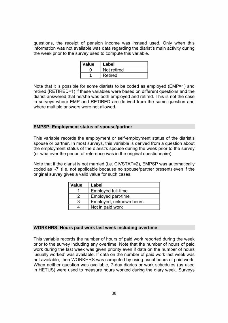
38
questions, the receipt of pension income was instead used. Only when this information was not available was data regarding the diarist’s main activity during the week prior to the survey used to compute this variable.
Value Label 0 Not retired 1 Retired
Note that it is possible for some diarists to be coded as employed (EMP=1) and retired (RETIRED=1) if these variables were based on different questions and the diarist answered that he/she was both employed and retired. This is not the case in surveys where EMP and RETIRED are derived from the same question and where multiple answers were not allowed.
EMPSP: Employment status of spouse/partner This variable records the employment or self-employment status of the diarist’s spouse or partner. In most surveys, this variable is derived from a question about the employment status of the diarist’s spouse during the week prior to the survey (or whatever the period of reference was in the original questionnaire). Note that if the diarist is not married (i.e. CIVSTAT=2), EMPSP was automatically coded as ‘-7’ (i.e. not applicable because no spouse/partner present) even if the original survey gives a valid value for such cases.
Value Label 1 Employed full-time 2 Employed part-time 3 Employed, unknown hours 4 Not in paid work
WORKHRS: Hours paid work last week including overtime This variable records the number of hours of paid work reported during the week prior to the survey including any overtime. Note that the number of hours of paid work during the last week was given priority even if data on the number of hours ‘usually worked’ was available. If data on the number of paid work last week was not available, then WORKHRS was computed by using usual hours of paid work. When neither question was available, 7-day diaries or work schedules (as used in HETUS) were used to measure hours worked during the diary week. Surveys
39
in which this variable does not represent hours worked last week should be documented in the README documents. The variable includes reported hours of paid work for any diarist who answered the question. For example, if the number of hours of work were asked to people who reported their economic activity status as ‘not working’, then the diarists’ answer should be included in this variable. The README file documents if all or only a subset of the diarists were asked the question. Values of 0 mean that the diarist reported zero hours of paid work. If diarists were not asked the question, they were given a value of -9 or -7 as appropriate. If diarists did not answer the question, they were coded as -8 for this variable.
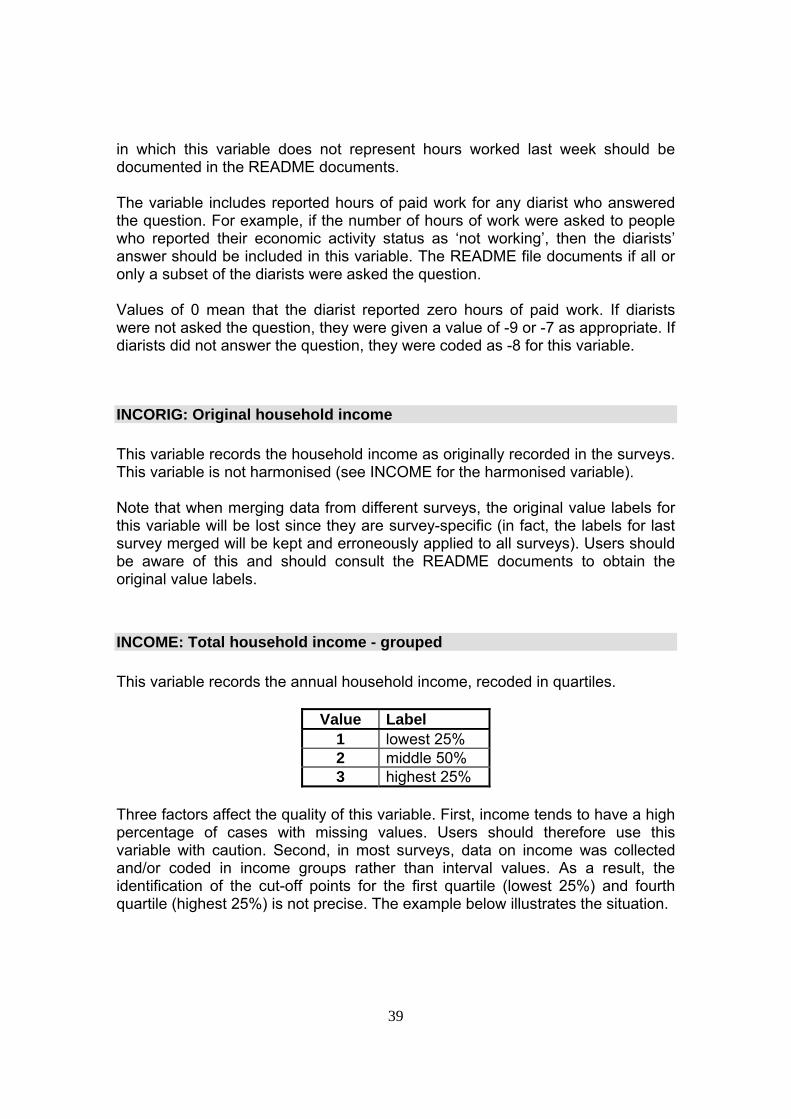
INCORIG: Original household income This variable records the household income as originally recorded in the surveys. This variable is not harmonised (see INCOME for the harmonised variable). Note that when merging data from different surveys, the original value labels for this variable will be lost since they are survey-specific (in fact, the labels for last survey merged will be kept and erroneously applied to all surveys). Users should be aware of this and should consult the README documents to obtain the original value labels.
INCOME: Total household income - grouped This variable records the annual household income, recoded in quartiles.
Value Label 1 lowest 25% 2 middle 50% 3 highest 25%
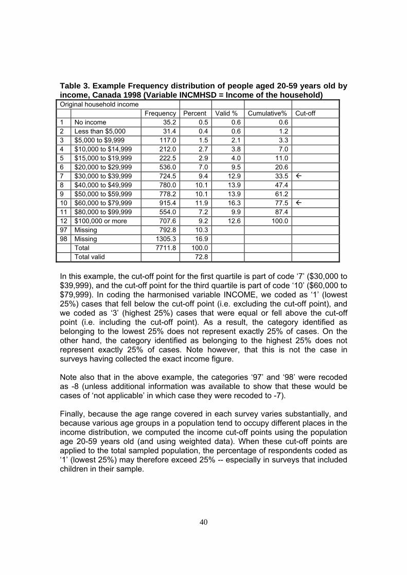
Three factors affect the quality of this variable. First, income tends to have a high percentage of cases with missing values. Users should therefore use this variable with caution. Second, in most surveys, data on income was collected and/or coded in income groups rather than interval values. As a result, the identification of the cut-off points for the first quartile (lowest 25%) and fourth quartile (highest 25%) is not precise. The example below illustrates the situation.
40
Table 3. Example Frequency distribution of people aged 20-59 years old by income, Canada 1998 (Variable INCMHSD = Income of the household) Original household income Frequency Percent Valid % Cumulative% Cut-off 1 No income 35.2 0.5 0.6 0.6 2 Less than $5,000 31.4 0.4 0.6 1.2 3 $5,000 to $9,999 117.0 1.5 2.1 3.3 4 $10,000 to $14,999 212.0 2.7 3.8 7.0 5 $15,000 to $19,999 222.5 2.9 4.0 11.0 6 $20,000 to $29,999 536.0 7.0 9.5 20.6 7 $30,000 to $39,999 724.5 9.4 12.9 33.5 8 $40,000 to $49,999 780.0 10.1 13.9 47.4 9 $50,000 to $59,999 778.2 10.1 13.9 61.2 10 $60,000 to $79,999 915.4 11.9 16.3 77.5 11 $80,000 to $99,999 554.0 7.2 9.9 87.4 12 $100,000 or more 707.6 9.2 12.6 100.0 97 Missing 792.8 10.3 98 Missing 1305.3 16.9 Total 7711.8 100.0 Total valid 72.8 In this example, the cut-off point for the first quartile is part of code ‘7’ ($30,000 to $39,999), and the cut-off point for the third quartile is part of code ‘10’ ($60,000 to $79,999). In coding the harmonised variable INCOME, we coded as ‘1’ (lowest 25%) cases that fell below the cut-off point (i.e. excluding the cut-off point), and we coded as ‘3’ (highest 25%) cases that were equal or fell above the cut-off point (i.e. including the cut-off point). As a result, the category identified as belonging to the lowest 25% does not represent exactly 25% of cases. On the other hand, the category identified as belonging to the highest 25% does not represent exactly 25% of cases. Note however, that this is not the case in surveys having collected the exact income figure. Note also that in the above example, the categories ‘97’ and ‘98’ were recoded as -8 (unless additional information was available to show that these would be cases of ‘not applicable’ in which case they were recoded to -7).
Finally, because the age range covered in each survey varies substantially, and because various age groups in a population tend to occupy different places in the income distribution, we computed the income cut-off points using the population age 20-59 years old (and using weighted data). When these cut-off points are applied to the total sampled population, the percentage of respondents coded as ‘1’ (lowest 25%) may therefore exceed 25% -- especially in surveys that included children in their sample.
41
EMPINCLM: Original monthly income from employment or self-employment This variable records the monthly personal income from wages/employment/self-employment during the last month. This variable is not harmonised and is instead recorded in national currency. Note that if data is only available on the personal income from wages/employment/self-employment during the last 12 months, this was converted in months and was documented in the README file. Note that when merging data from different surveys, the original value labels for this variable will be lost since they are survey-specific (in fact, the labels for last survey merged will be kept and erroneously applied to all surveys). Users should be aware of this and should consult the README documents to obtain the original value labels.
EDUCA: Educational level-original study code This variable contains the diarists’ education level as originally coded in the surveys. This variable is not harmonised. Note that value labels for the variable EDUCA are excluded from the dataset merging all surveys (but not in individual World5.5 files). In surveys for which the information on the diarist’s education was recorded in more than one variable, combinations of variables were used to create a single EDUCA variable. Note that when merging data from different surveys, the original value labels for this variable will be lost since they are survey-specific (in fact, the labels for last survey merged will be kept and erroneously applied to all surveys). Users should be aware of this and should consult the README documents to obtain the original value labels.
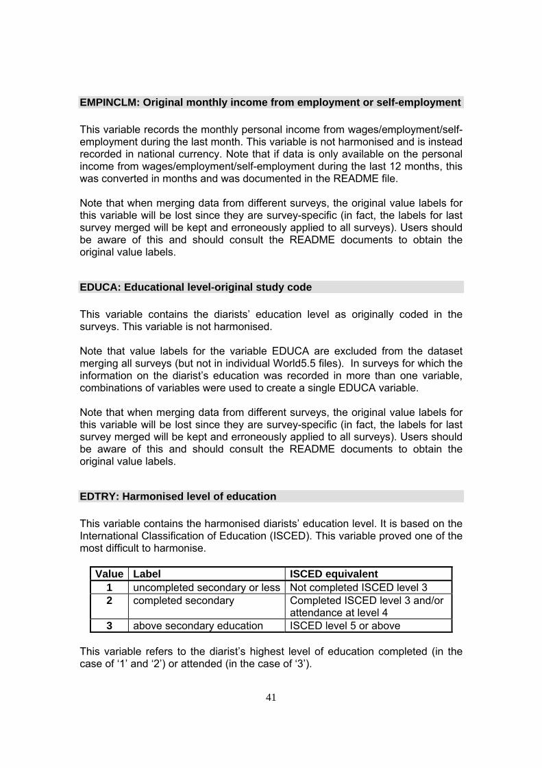
EDTRY: Harmonised level of education This variable contains the harmonised diarists’ education level. It is based on the International Classification of Education (ISCED). This variable proved one of the most difficult to harmonise.
Value Label ISCED equivalent 1 uncompleted secondary or less Not completed ISCED level 3 2 completed secondary Completed ISCED level 3 and/or
attendance at level 4 3 above secondary education ISCED level 5 or above
This variable refers to the diarist’s highest level of education completed (in the case of ‘1’ and ‘2’) or attended (in the case of ‘3’).

42
More information regarding the ISEC classification can be found in the following document: http://www.unesco.org/education/information/nfsunesco/doc/isced_1997.htm
Other harmonised information • DISAB • URBAN
DISAB: Diarist has a disability or long-term limiting health condition This variable indicates whether or not the diarist has a disability or long-term health limiting condition.
Value Label 0 No 1 Yes
It should be noted that the way disability is defined tends to vary across surveys, which may affect the degree of cross-survey comparability.
URBAN: Urban or rural household This variable indicates whether or not the diarist lives in an urban area.
Value Label 1 Urban/suburban 2 Rural/semi-rural
The survey-specific definition of ‘urban’ and ‘rural’ is included in the README file.
43
CHAPTER 4: WEIGHTS IN MTUS Two types of weights are needed for the analysis of time use data. First, as in all surveys, weights are needed to bring the sample in line with the population from which it was drawn. This involves taking into account the sample design, the over-sampling of specific sub-groups, non-responses, etc. We refer to this first type of weights as the ‘Population weights’. Secondly, weights are also needed to take into account seasonal variations and daily variations in patterns of time use. Even though most recent surveys have spread their data collection over the 12 months of the year and over the 7 days of the week, the resulting samples do not necessarily contain an equal number of every day of the year or an equal number of every day of the week. If the analyst is interested in computing accurate yearly averages, or accurate weekly averages, weights are therefore needed to correct for these sampling issues. We refer to this second type of weights as the ‘Day weights’. Below, we further discuss the availability and nature of weights in MTUS and discuss the procedures adopted in cases for which weights were not provided by the statistical agencies in charge of administrating the surveys.
4.1 Weights in earlier World5 versions All the weights in earlier versions of the Multinational Time Use Study were post-hoc types, that is, weights that were computed by the MTUS team as opposed to ‘original’ weights computed by the statistical agencies in charge of administering each survey. These post-hoc weights were age-sex-employment specific. They were computed based on official data published in the International Labour Office (ILO) Year Book of Labour Statistics. In the World5.5 version of the dataset, we relied mainly on “original” weights as computed by the statistical agencies. As described below, we computed post-hoc weights only when the original weights were not available.

44
4.2 Weights in World5.5 In World5.5, we implemented two major changes. First, we included the original weights when available, and second, we computed a new series of post-hoc weights that were age-sex specific rather than age-sex-employment specific (when needed). The reason for excluding employment from the computation of these post-hoc weights is related to inconsistencies in the definition of the active and non-active population in MTUS and in the ILO Yearbook of Labour Statistics. In World5.5, post-hoc weights were computed using data from the United Nations World Population Prospects or the ILO Yearbook of Labour Statistics (though when we used the latter, we used only age and sex group and not employment status). The following weights are included in World5.5:
OPOPWT: Original population weights that correct for over- and/or under-sampling but that do not correct for the day of the week;
ODAYWT: Original day weights that correct for over or under-sampling
of the different days of the week but that do not correct for population sampling;
OCOMBWT: Original combined weights that correct for both
population sampling and the day of the week.
POPWT2: Sex-age specific population post-hoc weights DAYWT2: Sex-age specific day post-hoc weights
PROPWT: Proposed weights (i.e. the weights that most Users will be
interested in, see below for details). An overview of the weights available in each survey in World5.5 is provided in Table 4.1.

45
Table 4.1 Overview of the availability of weights in World5.5
Country/Year OPOPWT ODAYWT OCOMBWT POPWT2 DAYWT2 PROPWT Australia 1987 √ √ Australia 1992 √ √ Australia 1997 √ √ Austria 1992 √ √ √ Canada 1971 √ √ √ Canada 1981 √ √ √ Canada 1986 √ √ Canada 1992 √ √ Canada 1998 √ √ Denmark 1964 √ √ Finland 1979 √ √ Finland 1987 √ √ Finland 2000 √ √ France 1985 √ √ France 1999 √ √ Germany 1992 √ √ Italy 1989 √ √ √ Netherlands 1975-95 √ √ Netherlands 2000 √ √ Norway 1971 √ √ √ Norway 1981 √ √ √ Norway 1990 √ √ √ Norway 2000 √ √ Slovenia 2000 √ √ South Africa 2000 √ √ √ Sweden 1991 √ √ √ UK 1961 √ √ UK 1974 √ √ UK 1983 √ √ UK 1987 √ √ √ UK 1995 √ √ √ UK 2000 √ √ USA 1965 √ √ USA 1975 √ √ USA 1985 √ √ USA 1992 √ √ USA 1998 √ √ USA 2003 √ √ As mentioned, most users will use PROPWT which corrects for both population and day sampling issues. Note that some surveys inflate the sample size by a factor to mirror the size of the whole population of the country. Such an inflation is useful if the aim of the analysis is to provide an absolute value of the number of people with specific
46
characteristics. For this reason, if the original weights are inflated, the OCOMBWT or OPOPWT should be left inflated. Nevertheless, to promote consistency among the datasets and to prevent surveys from countries with larger populations from apparently swamping surveys from countries with smaller populations, we deflate the original weight in the computation of PROPWT. The mean of the original weight will sum to the inflation factor. Where survey designs collect diaries on a weekday and a weekend day, it is advisable to use the mean of the weekday diaries to deflate weekday diaries and the mean of the original weight for the weekend diaries to deflate the weekend diaries. In PROPWT, we adjusted the weights by using the mean weight for the total sample. When carrying multivariate analysis, Users may want to readjust the weights by using the mean weight for the sub-sample analysed in order to obtain more accurate standard errors. Note also that the data as weighted by PROPWT above should result in a perfect distribution of diaries across the 7 days of the week. However, when the analysis is carried out on sub-samples, the distribution is oftentimes imperfect – even if original weights are used. It may therefore be a good idea to request a frequency distribution after turning the weights on in order to see how perfect or imperfect is the resulting distribution. Users may also, if they wish so, compute a further correction to obtain a perfect distribution by day of the week (see the details in the next section).
4.3 About the computation of post-hoc weights We provide below examples of how post-hoc weights were computed. Example 1: Computation of POPWT2 POPWT2 was computed by using data on the population by 5-year age group and sex and published by the United Nations in World Population Prospects. In this publication, the data is available for each year ending with a ‘0’ or a ‘5’. We used the closest year to the survey year. The weight POPWT2 results from the comparison of the sampled distribution of the population by sex and age (in the survey) and the observed distribution of the population as estimated by the United Nations. POPWT2 = Observed / Sampled.
47
For example, let us assume that the male population aged 20-24 represented 5.2 percent of the total population according to the United Nations’ estimates but only 3.4 percent in the sample. POPWT2 is a correction factor equal to 5.2 divided by 3.4 = 1.53. Since the sample under-estimates this population sub-group, each individual should represent 1.53 cases instead of only 1 case. Conversely, if a sub-group was over-sampled, it would be assigned a value for POPWT2 less than 1. Note that this is a zero-sum ‘game’ and the average value of the weights across the sampled population is 1.0. Example 2: Computation of DAYWT2 DAYWT2 was computed by comparing the sampled distribution of diaries by the day of the week by sex and age (in the survey) and the expected distribution in which each day of the week represents 1/7th of the total number of diaries. DAYWT2 = Expected / Sampled. For example, let us assume that 15 diaries were filled in on Mondays by the male population aged 20-24 out of a total of 140 diary days (10.7 percent) instead of the expected 20 diary days (20/140 = 1/7 = 14.3 percent). DAYWT2 is a correction factor equals to 14.3 divided by 10.7 = 1.34. Since the sample under-estimates the number of Mondays, each diary filled in on a Monday represents 1.34 diaries instead of only 1. Conversely, if a day of the week was over-sampled, it would result in a value of DAYWT2 less than 1. Note that this is a zero-sum ‘game’ and the average value of the weights across the sampled population is 1.0. Example of syntax to compute DAYWT2 (in SPSS): compute DAYWT2 = $sysmis. sort cases by SEX AGEGR DAY. aggregate out='R:\Soci1205\Master Folder\Work Files\Junk\Aus92-12.tmp' /break=SEX AGEGR DAY /DAYCOUN2=n. aggregate out='R:\Soci1205\Master Folder\Work Files\Junk\Aus92-21.tmp' /break=SEX AGEGR /WKCOUNT2=n. execute. match files file=* /table='R:\Soci1205\Master Folder\Work Files\Junk\Aus92-12.tmp' /by SEX AGEGR DAY. match files file=* /table='R:\Soci1205\Master Folder\Work Files\Junk\Aus92-21.tmp' /by SEX AGEGR. compute DAYWT2 eq (WKCOUNT2/7)/DAYCOUN2. execute. variable label DAYWT2 'Age/gender specific day weights'.

48
4.4 About PROPWT PROPWT is the weight that is suggested for use to Users. In theory, it corrects perfectly for the day of the week. However, in practice the correction may not be perfect when analysing specific subgroups of respondents. A similar syntax to that explained above should be used if Users want to further correct the data to obtain a perfect distribution of cases across the seven days of the week. PROPWT was computed as follows: If no weights were provided in the original file, PROPWT = POPWT2 * DAYWT2. If a combined weight (correcting for both population and day sampling) was available in the original file, PROPWT = OCOMBWT Or PROPWT = OCOMBWT / mean of OCOMBWT (if OCOMBWT inflated the original number of cases). If an original population weight was available but no day weight, PROPWT = OPOPWT * DAYWT2 Or PROPWT = (OPOPWT/mean) * DAYWT2 (if OPOPWT inflated the original number of cases).
49
CHAPTER 5: THE ANALYSIS OF TIME-USE DATA Written with the special collaboration of Dr. Donna Dosman (University of Alberta) In this chapter, we provide information to Users concerning the analysis of time-use data. We cover the basic statistics that are routinely computed using time-use data, and discuss the multivariate analysis of such data, drawing attention to some special characteristics of time-use data. It should be noted that this chapter is restricted to the analysis of summary time-use data and does not cover the analysis of episode data.
5.1 Descriptive analysis Three main types of statistics are usually computed when analysing time-use data:
Mean time spent on each activity by the total population or by specific sub-groups (T);
Participation rates (i.e. proportion of people having spent at least 1
minute on the specified activity) (P);
Mean time spent on each activity by participants only (M) Where T = P * M. Below is an example in SPSS of how to compute these statistics. Example of SPSS syntax to compute key descriptive statistics ***** * Computation of mean time spent on specified activities by the total sample and various sub-groups ***** TITLE ‘Mean value of AV1 and AV10 for the total sample’. DESCRIPTIVES VARIABLES= AV1 AV10 /STATISTICS=MEAN STDDEV MIN MAX . TITLE ‘Mean value of AV1 and AV10 by sex’.
50
MEANS TABLES= AV1 AV10 BY SEX /CELLS MEAN COUNT. TITLE ‘Mean value of AV1 and AV10 by FAMSTAT and sex’. SORT CASES BY SEX. SPLIT FILE LAYERED BY sex . MEANS TABLES= AV1 AV10 BY famstat /CELLS MEAN COUNT. SPLIT FILE OFF. ****** * Computation of participation rates for the variable AV1 ******* Compute pav1 = $sysmis. If (AV1 ge 1) pav1 =1. If (AV1 eq 0) pav1 = 0. DESCRIPTIVES VARIABLES= pav1 /STATISTICS=MEAN STDDEV MIN MAX . ***** * Computation of time spent on specified activities by participants only ******* temporary. Select if (pav1 =1). DESCRIPTIVES VARIABLES= AV1 /STATISTICS=MEAN STDDEV MIN MAX . ****** The above statistics may also be computed to distinguish weekdays and weekends, or various other characteristics of respondents. About the participation rates: in the case of 1-day diary surveys, there may be a large proportion of non-respondents on any diary day. These may be people who happened not to be spending any time on a specific activity on the diary-day, or people who never spend any time on a specific activity. Note that the proportion of respondents (or non-respondents) obtained on the basis of surveys that used a 7-day diary as opposed to a 1-day diary may be different if the data is

51
averaged over the 7 days of the week (as it is currently the case with the Dutch surveys). This is because the likelihood that a respondent does not spend any time on a specific activity is much lower in the case of a 7-day diary than in the case of a 1-day diary. This should be kept in mind when carryout out comparative analyses.
5.2 Multivariate analysis Users may be interested in analysing the determinants of time spent on specific activities and will therefore be running multivariate analysis. And while statistical packages may allow Users to easily run basic regression models, it is important to keep in mind that the nature of time-use data is such that several key assumptions at the basis of the general lineal model are violated. Below, we review some of these key statistical assumptions.1
5.2.1 The Normality assumption The general linear model assumes that the error terms have a normal distribution (normality assumption) with a mean of zero.
Fundamental to this assumption is the requirement that the sample is random and that the dependent variable is normally distributed. Analysis of time use data often violates this assumption because of the typical large number of ‘zeros’, i.e. cases that spent 0 minutes on the specific activity. For example, while on any single day the large majority of people are expected to sleep and eat, this is not the case when it comes to activities such as volunteering or participating in a sport. The difficulty here is that the ‘zeros’ encompass both ‘real’ zeros, that is people who never participate in an activity, and zeros that result from people who happened not to participate in the specific activity on the diary day, but who normally do participate in the activity in the course of their lives. As mentioned above, the normality assumption is usually not violated for activities that are carried out by a very large proportion of the population, such as sleeping, eating, or watching television (i.e. activities for which the participation rate is close to 1 on the diary day). However, many time-use activities have a large proportion of non-participants. As explained above, the non-participants may be people who happened not to be spending any time on a specific activity on the diary-day, or people who never spend any time on a specific activity. When the value of the participation rate is low, the normality assumption is likely to be violated.
1 There are of course other assumptions, but we focus here on those that are known to be particularly problematic in the analysis of time use data.
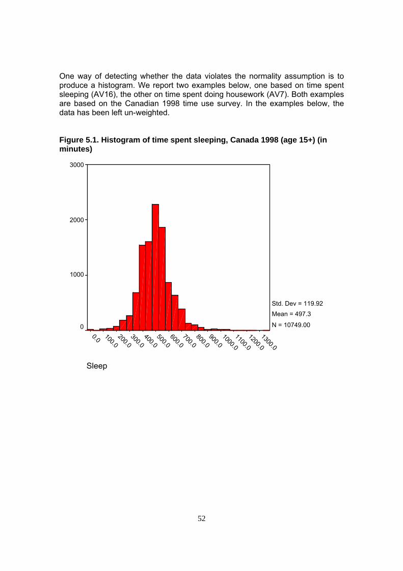
52
One way of detecting whether the data violates the normality assumption is to produce a histogram. We report two examples below, one based on time spent sleeping (AV16), the other on time spent doing housework (AV7). Both examples are based on the Canadian 1998 time use survey. In the examples below, the data has been left un-weighted. Figure 5.1. Histogram of time spent sleeping, Canada 1998 (age 15+) (in minutes)
Sleep
1300.0
1200.0
1100.0
1000.0
900.0800.0
700.0600.0
500.0400.0
300.0200.0
100.00.0
3000
2000
1000
0
Std. Dev = 119.92 Mean = 497.3
N = 10749.00

53
Figure 5.2. Histogram of time spent doing routine housework, Canada 1998 (age 15+) (in minutes)
Housework
750.0700.0
650.0600.0
550.0500.0
450.0400.0
350.0300.0
250.0200.0
150.0100.0
50.00.0
7000
6000
5000
4000
3000
2000
1000
0
Std. Dev = 79.75 Mean = 46.4
N = 10749.00
Textbooks often refer to the so-called ‘robustness’ of the general linear model to deviations from the normality assumption. It must however be kept in mind here that the deviations in the case of time use data may be very large, especially for activities that have a large proportion of non-participants. In order to further illustrate this point, we carried out a simple OLS (Ordinary least-squares) regression using HOUSEWORK as the dependent variable. We used age, gender, and the number of children as our independent variables. Results appear below, including a plot of the residuals. Example of a SPSS syntax commands to carry out a OLS regression compute men=$sysmis. if (sex eq 1) men =1. if (sex eq 2) men =0. REGRESSION
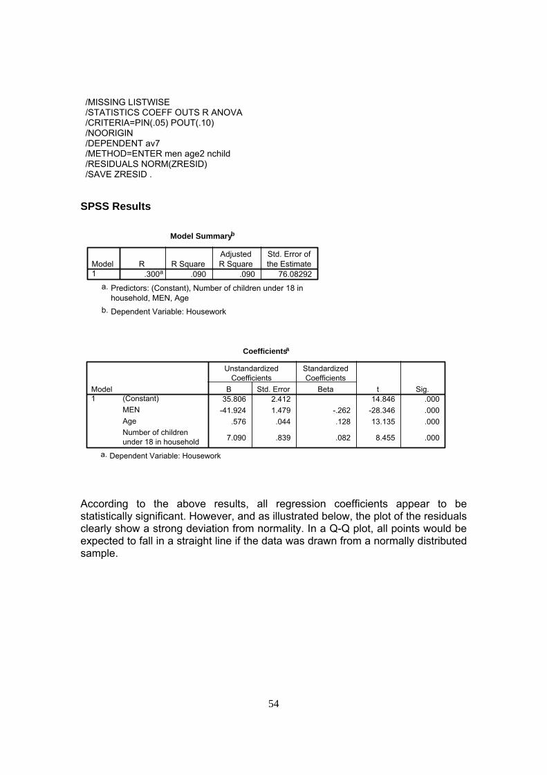
54
/MISSING LISTWISE /STATISTICS COEFF OUTS R ANOVA /CRITERIA=PIN(.05) POUT(.10) /NOORIGIN /DEPENDENT av7 /METHOD=ENTER men age2 nchild /RESIDUALS NORM(ZRESID) /SAVE ZRESID . SPSS Results
Model Summaryb
.300a .090 .090 76.08292Model1
R R SquareAdjustedR Square
Std. Error ofthe Estimate
Predictors: (Constant), Number of children under 18 inhousehold, MEN, Age
a.
Dependent Variable: Houseworkb.
Coefficientsa
35.806 2.412 14.846 .000-41.924 1.479 -.262 -28.346 .000
.576 .044 .128 13.135 .000
7.090 .839 .082 8.455 .000
(Constant)MENAgeNumber of childrenunder 18 in household
Model1
B Std. Error
UnstandardizedCoefficients
Beta
StandardizedCoefficients
t Sig.
Dependent Variable: Houseworka.
According to the above results, all regression coefficients appear to be statistically significant. However, and as illustrated below, the plot of the residuals clearly show a strong deviation from normality. In a Q-Q plot, all points would be expected to fall in a straight line if the data was drawn from a normally distributed sample.
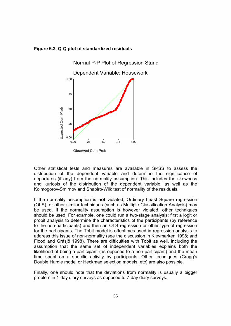
55
Figure 5.3. Q-Q plot of standardized residuals
Normal P-P Plot of Regression Stand
Dependent Variable: Housework
Observed Cum Prob
1.00.75.50.250.00
Exp
ecte
d C
um P
rob
1.00
.75
.50
.25
0.00
Other statistical tests and measures are available in SPSS to assess the distribution of the dependent variable and determine the significance of departures (if any) from the normality assumption. This includes the skewness and kurtosis of the distribution of the dependent variable, as well as the Kolmogorov-Smirnov and Shapiro-Wilk test of normality of the residuals.
If the normality assumption is not violated, Ordinary Least Square regression (OLS), or other similar techniques (such as Multiple Classification Analysis) may be used. If the normality assumption is however violated, other techniques should be used. For example, one could run a two-stage analysis: first a logit or probit analysis to determine the characteristics of the participants (by reference to the non-participants) and then an OLS regression or other type of regression for the participants. The Tobit model is oftentimes used in regression analysis to address this issue of non-normality (see the discussion in Klevmarken 1998; and Flood and Gråsjö 1998). There are difficulties with Tobit as well, including the assumption that the same set of independent variables explains both the likelihood of being a participant (as opposed to a non-participant) and the mean time spent on a specific activity by participants. Other techniques (Cragg’s Double Hurdle model or Heckman selection models, etc) are also possible. Finally, one should note that the deviations from normality is usually a bigger problem in 1-day diary surveys as opposed to 7-day diary surveys.
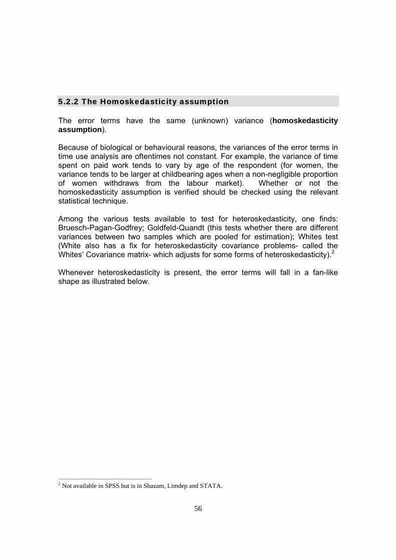
56
5.2.2 The Homoskedasticity assumption The error terms have the same (unknown) variance (homoskedasticity assumption). Because of biological or behavioural reasons, the variances of the error terms in time use analysis are oftentimes not constant. For example, the variance of time spent on paid work tends to vary by age of the respondent (for women, the variance tends to be larger at childbearing ages when a non-negligible proportion of women withdraws from the labour market). Whether or not the homoskedasticity assumption is verified should be checked using the relevant statistical technique. Among the various tests available to test for heteroskedasticity, one finds: Bruesch-Pagan-Godfrey; Goldfeld-Quandt (this tests whether there are different variances between two samples which are pooled for estimation); Whites test (White also has a fix for heteroskedasticity covariance problems- called the Whites’ Covariance matrix- which adjusts for some forms of heteroskedasticity).2 Whenever heteroskedasticity is present, the error terms will fall in a fan-like shape as illustrated below.
2 Not available in SPSS but is in Shazam, Limdep and STATA.
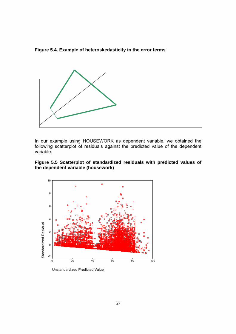
57
Figure 5.4. Example of heteroskedasticity in the error terms
In our example using HOUSEWORK as dependent variable, we obtained the following scatterplot of residuals against the predicted value of the dependent variable. Figure 5.5 Scatterplot of standardized residuals with predicted values of the dependent variable (housework)
Unstandardized Predicted Value
100806040200
Sta
ndar
dize
d R
esid
ual
10
8
6
4
2
0
-2
58
As can be seen, on average, the dispersion (variance) of the residuals is larger for high values of the predicted dependent variable than for small values. When heteroskedasticity is present the OLS estimates will no longer be BLUE (best linear unbiased estimators). In particular, the usual tests of statistical significance (such as t-test) will not be valid. Some of the solutions to this problem include the White’s Covariance structure, or weighted least squares.
5.2.3 The Independence assumption There are in fact two different assumptions about independence. One is that the independent variables are to be independent of the error term derived from the regression. The covariance Cov(Xt , µt) = 0. This assumption is usually referring to problems of collinearity.3 The second assumption is that any two observations should be independent, i.e. Cov (εi,εj)=0. In time series data where this period’s observation is based on last period’s observation, the problem is called autocorrelation. This independence assumption is often violated when multiple day diaries are captured from one respondent or when there is more than one respondent from each household. Some of the solutions to this problem of non-independence of the cases include:
One ‘radical’ solution is to randomly select only 1 diary day per respondent, or to randomly select only 1 respondent per household. This solves the problem of non-independence between observations, but results in a loss of the number of cases.
Another potential solution for multiple day diaries is to create a
composite weekly measure of time spent in activities. With this measure of a broader time period, fewer of the above assumptions should be violated. Conversion of the daily diaries into weekly measures depends on the number of observations per respondent.
In datasets which have observations for more than one household
member, it is also possible to model the time use patterns as household patterns. The key here is that the dependent variable needs
3 Collinearity is often a problem in social science estimation. It arises when each variable is capturing the effect of the other variables. It usually results in a high value of r –square but low t-statistics for each regression coefficient. Multicollinearity may be detected by looking at the bivariate correlation between independent variables, and by computing VIF and condition index. One solution is to re-specify the regression model with fewer variables. A Lagrange multiplier test or likelihood ratio test may be used to test the significance of models with and without the ‘problem’ variables.

59
to be converted into a household measure and the resulting variable treated as the dependent variable.
SPSS version 11.0 has also a new feature for regression models with
correlated random effects (check under ‘mixed model).
5.2.4 Other possible statistical problems in time-use analysis Time spent on any activity has a minimum of zero and a maximum of 1440 minutes (24 hours). Users should be aware that some regression models may produce out-of-range estimates, for example negative value of time spent on a specific activity, or more than 24 hours.

60
Bibliography Note that there is a large literature on time use. We report below only selected titles that directly address some of the methodological issues raised in this User's Guide. Fisher, K. (2000). Details of Time Use Studies and On-Line Documentation,
Release 2, 30 June, 2000. Institute for Social and Economic Research, University of Essex (Colchester, UK).
Flood, Lennart; Gråsjö, Urban (1998).
http://www.unites.uqam.ca/ideas/data/Papers/hhsgunwpe0005.html Regression Analysis and Time Use Data A Comparison of Microeconometric Approaches with Data from the Swedish Time Use Survey (HUS).
Gershuny, J. (2000). Changing Times: Work and Leisure in Postindustrial
Society. (Oxford: Oxford University Press). Juster, F.T. and F.P. Stafford (eds). Time, Goods, and Well-Being. (Ann Arbor,
MI: Institute for Social Research). Juster, F.T., Stafford, F.P. (1991). 'The allocation of time: empirical findings,
behavioral models, and problems of measurement'. Journal of Economic Literature. XXIX: 471-522.
Klevmarken, Anders (1998). Microeconomic Analysis of Time-use Data. Did we
reach the promised land? Working Paper Series, Department of Economics, Uppsala University.
Knulst, W., Van den Broek, A. (1998). 'Do time-use surveys succeed in
measuring 'busyness'? Some observations of the Dutch case'. Society and Leisure. 21, 2: 563-72.
Pentland, W.E., Harvey, A.S., Lawton, M.P. (eds.) (1999). Time-Use Research in
the Social Sciences. (New York: Plenum Press). Robinson, J.P., Godbey, G. (1997). Time for Life; The Surprising Ways
Americans Use Their Time. (College Park, PA: Pennsylvania State University Press).
Szalai, A. (ed.) (1972). The Use of Time: Daily Activities of Urban and Suburban
Populations in Twelve Countries. (Paris: Mouton).
61
APPENDIX : README Files for Each Country
Australia 1987, 1992, 1997 Austria 1992 Canada 1971/72, 1981, 1986, 1992, 1998 Denmark 1964 Finland 1979, 1987/88, 1999 France 1998 Germany 1991/92 Italy 1989 The Netherlands 1975, 1980, 1985, 1990, 1995 , 2000 Norway 1971, 1981, 1990/91, 2000 Slovenia 2000 South Africa 2000 Sweden 1990/91, 2000 UK 1961, 1974/75, 1983, 1987, 1995, 2000 USA 1965/66, 1975/76, 1985, 1992/94, 1998, 2003