Multinational firms’ organisational dynamics*

Leandro Navarro†

July 18, 2021

Link to the latest version

Abstract

I analyse the organisational choices of heterogeneous firms in a model of incomplete contracts

under uncertainty about foreign institutions. Under institutional uncertainty, only the most productive

firms offshore production but other firms sequentially follow as uncertainty reduces through learning.

The process intensifies competition among final good firms, which impacts the optimal organisation

of the firm: firms initially choose vertical integration, but the stronger competition tilts the balance

towards outsourcing. Thus, the least productive offshoring firms sequentially shift to outsourcing.

A test with sector-level data for the US manufacturing sectors provides supportive evidence of the

model’s main predictions.

Keywords: Multinational firms, incomplete contracts, global sourcing, uncertainty, institutional shocks.

JEL: D23, D81, D83, F14, F23

1 Introduction

The increasing importance of intermediate inputs in international trade and the growing role of multina-

tional firms in the organisation of global value chains have captured the attention of many scholars.1 A

growing literature on global sourcing has focused on the determinants of firms’ organisational choices

under incomplete contracts, with a particular emphasis on the role of institutions in the organisation of

*I am grateful to Philip Saure for his supervision and support. I thank to Aksel Erbahar, Christian Fischer, Victor Gimenez-Perales, Philipp Harms, Philipp Herkenhoff and Mario Larch and all participants at the Johannes Gutenberg University Mainzworkshop, University of Buenos Aires seminar, and University of Hagen conference for valuable comments and discussion.All errors are my own.

†Johannes Gutenberg University Mainz. Email: lenavarr@uni-mainz.de. Johannes-von-Muller-Weg 2, Office 01-421.Mainz (55118), Germany.

1Grossman and Helpman (2002, 2004, 2005); Antras and Helpman (2004); Helpman (2006); Alfaro and Charlton (2009);Johnson and Noguera (2012); Antras and Chor (2013). For literature review, see Antras (2015) and Antras and Chor (2021).

1

supply chains.2 Recent events, such as Brexit and US-China trade war, have intensified the attention

on the consequences of those events in the reorganisation of global value chains and the relocation of

suppliers to new countries.3

Firms face uncertainty about institutional conditions when deciding on reorganising the supply chains

to new foreign sourcing locations. For example, when firms lack previous experience in foreign coun-

tries, they form beliefs about institutional conditions by using external information sources and observing

other firms active in those locations. Institutional uncertainty also emerges when foreign governments

announce the implementation of deep institutional reforms, but firms do not fully believe in the scope of

the reforms.

I extend a model of global sourcing to analyse the effects of institutional uncertainty on the organisa-

tional dynamics of global value chains.4 In the model, the presence of uncertainty implies that, initially,

only the most productive firms in the market explore offshoring. These firms’ actions reveal informa-

tion about the foreign institutions (information externalities), allowing other firms to learn and reduce

their prior uncertainty. As more firms explore their offshoring potential, more information is revealed.

Uncertainty progressively erodes, and more firms sequentially follow, resulting in a progressive expan-

sion of the sectoral offshoring activity. The model predicts that the lower prices of the offshoring firms

cause a progressive increase in the competition intensity in the final goods market, which impacts the

dynamic organisational structure of the supply chains.5 On the offshoring side, the more intense compe-

tition implies that the least productive firms among the vertically integrated offshoring firms sequentially

reorganise the supply chains to arm’s length trade.

The baseline model of global sourcing defines two countries (North-South) and multiple differenti-

ated final good sectors.6 As in Antras and Helpman (2004), the final good producers are located in the

North, and they can decide on contracting either with northern or southern manufacturers to supply the

intermediate inputs. The location dimension of the decision balances the trade-off between exploiting

the advantage of lower marginal costs in the South to produce intermediate inputs and the higher or-

ganisational fixed costs of offshore operations. Under incomplete contracts, the sourcing decision also

involves an organisational dimension (integration vs outsourcing). It balances the trade-off between min-2See Antras and Helpman (2008); Yeaple (2006); Levchenko (2007); Nunn (2007); Nunn and Trefler (2013). For the

analysis of the role of FTAs and multilateral agreements on the organisation of global value chains, see Ornelas and Turner(2008, 2012); Antras and Staiger (2012); Ornelas et al. (2020); Handley et al. (2020).

3See Head and Mayer (2019); Blanchard (2019); Van Assche and Gangnes (2019); Grossman and Helpman (2020); Gereffiet al. (2021) and Bown et al. (2021).

4For a close reference to the perfect information benchmark, see Antras and Helpman (2004).5Higher competition intensity in final goods market impacts on dynamic allocation of property rights along the value chain.6The characterisation of the benchmark perfect information equilibrium is based on a generalisation of the global sourcing

model in Antras and Helpman (2004). I discuss below the extent, features, and consequences of the generalisation.

2

imising the hold-up by vertical integration and increasing the per-period organisational fixed costs due

to managing a larger and more complex organisation.7

I characterise uncertainty about the institutional conditions in foreign locations as uncertainty in the

per-period organisational fixed costs of offshore operations. The northern final good producers face

uncertainty about the new institutional regime abroad, but they can learn from offshoring producers

and progressively reduce the prior uncertainty. As in Larch and Navarro (2021), in each period t, the

producers under domestic sourcing face a trade-off situation. They can delay exploring their offshoring

potential (i.e. wait) and receive new information that reduces the exploration risk. The delay involves

lower expected profits by sourcing domestically during the waiting period. If they explore, they have to

pay an offshoring sunk cost, and the institutional fundamentals are revealed to them.8 Thence, they can

choose with certainty the optimal organisational form. The sectoral equilibrium path is characterised by

a Markov decision process, in which the final good producers update their prior uncertainty through a

Bayesian learning mechanism.9

The main prediction of the model concerning the organisational dynamics is: the increase in off-

shoring activity progressively lowers the sector’s price index, implying a higher intensity in the competi-

tion in the final goods market. Thus, it induces a progressive vertical disintegration of the supply chains.

I call this prediction the first channel of the competition effect on vertical disintegration.10

Zooming in on the vertical disintegration dynamics, the model shows that the most productive final

good producers lead the offshoring exploration and initially choose foreign integration as the optimal

organisational form. However, as the competition in the final goods market endogenously intensifies, the

least productive among them begin to sequentially reorganise the supply chains to independent foreign

suppliers.11 To illustrate the process, consider the dynamic organisational path of one final good producer

H . Initially, the expected gains from waiting surpass the expected gains from exploring forH . Therefore,

H decides to wait under domestic sourcing. As other more productive final good producers explore7Different ownership structures lead to different distortions in ex-ante investments. The hold-up is minimised by the al-

location of property rights on the party that contributes more (Grossman and Hart, 1986; Hart and Moore, 1990). Aboutorganisational fixed costs, integrated structures impose additional costs due to the more complex structure of a larger and morediversified organisation (Grossman and Helpman, 2002). They are governance related to the integration of two independentparties into a hierarchical structure within the firm boundaries (Coase, 1937; Williamson, 1979, 1985).

8The offshoring sunk cost refers to feasibility studies that analyse all the possible organisational structures of offshoring inthe South. Thus, after paying it, they discover the institutional fundamentals in the foreign location for all the offshoring types.There is no remaining uncertainty for those producers. Nevertheless, it remains as private information to them.

9The characterisation of the learning mechanism and the exploration decision is based on Larch and Navarro (2021). Otherreferences are Rob (1991) and Segura-Cayuela and Vilarrubia (2008).

10Lower marginal costs in the South imply that, as more firms offshore, the competition in the final goods market intensifies.11Technically, the productivity cutoff for foreign integration has a non-monotonic behaviour over time. It decreases in early

periods of the dynamic offshoring path, as the leading final good producers choose foreign integration. In later periods, theproductivity cutoff increases as the more intensive competition in the final goods market deteriorates the benefits of integrationand induces a sequential vertical disintegration.

3

the offshoring potential, H receives new information, reducing H’s exploration risk. At a later date,

H finds it profitable to explore, pays the offshoring sunk cost and chooses foreign integration as the

optimal offshoring type. However, as the exploration sequence continues, the sectoral offshoring activity

increases and more producers exploit the marginal costs advantages of offshoring. Thus, the price index

progressively reduces and the competition in the final goods market intensifies, leading to a progressive

deterioration in the gains from integration. Eventually,H finds it more profitable to vertically disintegrate

the supply chain towards foreign outsourcing.12

I test the main theoretical prediction of the model, i.e. the first channel of the competition effect on

vertical disintegration, using sector-level data of US manufacturing sectors for the period 2002-2016. To

that aim, I use the related-trade party import data provided by the US Census Bureau, which distinguishes

import flows between related and non-related parties.13 To obtain information on the input-output rela-

tionships, I merge this data with the BEA input-output matrix linking the import data at the supplier

sector with the final good producer sectors that use these intermediate inputs in their respective produc-

tion processes. Additional data on the final good producer sectors comes from the manufacturing survey

of the US Census Bureau.14

I work with sector-level data. Thus, I aggregate the firm-level theoretical predictions of the model

to obtain the respective sector-level organisational dynamics. I derive a structural two-stage empirical

model that identifies the mechanism of the first channel of the competition effect on vertical disintegra-

tion. In the first stage, I derive a log-linear empirical model that estimates the effects of the final good

producer sector offshoring activity (offshoring share) on the respective final goods market price index.

In the second stage, I derive a fractional logit model that estimates the effect of the predicted changes in

the price index on the intra-firm intensity of the final good producer sector.15 The empirical results show

that an increase in a final good producer sector’s offshoring activity is associated with a reduction in the

respective price index. The latter, in turn, leads to a reduction in the intra-firm intensity of the sector.16

To analyse firms’ organisational dynamics in the context of location and relocation decisions of off-12On the domestic side, the increase in competition intensity leads to vertical disintegration of domestic supply chains.13The data on imports does not identify the type of integration (forward or backward). Therefore, I generalise the organisa-

tional choice model in Antras and Helpman (2004) by allowing for both types of integration. Thus, I derive firm and sectoralorganisational dynamics that allows me to overcome the data limitations. Nevertheless, I show that the model’s predictions arealso consistent with an organisational decision space as defined by Antras and Helpman (2004).

14I use Rauch (1999)’s classification of commodities to build differentiation indices for final good producer and suppliersectors. They reflect the intensity of the sectors in relationship-specific investments. i.e. the contract-dependency of the sectorand thus the exposure to hold-up (Nunn, 2007). For similar input-output matrix approach, see Antras (2015).

15The sector offshoring share captures the offshoring activity in the final good sector. It is computed by the total importsof the final good sector divided by the total sales of the respective sector. The intra-firm intensity measures the intensity ofintra-firm trade (i.e. imports from related parties) relative to the total sales of the final good sector.

16I also introduce a set of reduced-form empirical models that capture different features of the organisational dynamicsconsistent with the model’s theoretical predictions.

4

shore suppliers across heterogeneous foreign countries, I follow by extending the theoretical model to

multiple countries. In a multi-country setup under institutional uncertainty, information shocks (e.g.

institutional reforms) may cause the exploration of new countries and thus promote the relocation of

offshore suppliers across foreign locations. I analyse the case of a low-wage foreign country (East) that

experiences a favourable institutional information shock (e.g. generated by institutional reform). When

the shock impacts on the prior beliefs about eastern institutions, it may trigger a sequential offshoring

exploration to the East, resulting in a full or partial relocation of offshore (southern) suppliers to East. As

the sequential offshore relocation advances, it reduces the sector’s price index and increases the compe-

tition intensity in the final goods market. As in the two-country model, this effect leads to a progressive

vertical disintegration of the supply chains in the sector. I define the relocation of offshore suppliers to

low wage foreign countries as the second channel of the competition effect on vertical disintegration.

I test the prediction of the multi-country model by analysing the effects of a particular institutional

information shock: the accession of China to the WTO. The initial conditions are characterised by a

low wage of China with low market shares in US markets. To this aim, as before, I aggregate the firm-

level predictions of the model to sector-level organisational dynamics. I derive a structural model in two

stages that identifies the mechanism of the first and second channels of the competition effect on vertical

disintegration. The first stage estimates the effects of both channels, i.e. the sector offshoring activity

and the China market share on the sector’s intermediate inputs imports, on the respective price index.17

As before, the second stage estimates the effect of price index changes predicted by both channels of the

competition effect on the intra-firm intensity of the sector. In line with the theory, the results show that

the increase in the sector offshoring share and the increase in China’s market share in the imports of the

sector’s intermediate inputs reduce the sector price index. The reductions in the price index predicted by

both channels lead to vertical disintegration of the offshore supply chains.

I conclude by introducing a theoretical extension to the multi-country model that studies the role of

free-trade agreements (FTAs) and multilateral agreements (MAs) as institutional information shocks that

trigger the exploration of new locations under institutional uncertainty.18

The FTAs incorporate a set of rules and regulations that define the institutional framework in the

agreement, such as intellectual property and property rights protection, foreign investment, dispute reso-

lution mechanisms, environmental regulation, labour market regulation and mobility.19 The ratification17After controlling for the total offshoring activity of the sector, China’s market share in the final good sector’s imports

captures the relocation of offshore suppliers to China.18As predicted by the theory, the exploration of new countries by northern final good producers may increase the offshoring

activity and/or relocation processes of offshore suppliers across foreign countries. This extension focuses on the role of FTAsand MAs as triggers of the exploration sequences to new locations.

19See Maggi (1999), Dur et al. (2014), and Limao (2016). For examples of regulatory agreements involved in FTAs see

5

of a FTA reveals a commitment of the signing governments to provide an institutional environment that

meets the set of rules specified in the agreement. If those rules are observable by the final good produc-

ers, a new FTA impacts on the institutional beliefs about a partner country, leading to an improvement of

the previously pessimistic priors.20

Exploring further the institutional dimension of the FTAs, I also consider the role of FTAs among

third countries as institutional information shocks. I define them as those FTAs where the country of

the final good producers (North) is not involved. The model predicts that they may impact on priors

and trigger the exploration of new locations in the FTA by northern firms. The intuition is the follow-

ing: when a FTA is under negotiation, countries with good institutional fundamentals do not want to

expose themselves to trade with partners under poor institutional conditions, while countries with bad

institutional fundamentals may want to avoid committing to strict rules that they cannot enforce. Thus,

the institutional framework of the FTA emerges from bargaining on a set of rules among the members.

The final good producers from a non-member country may associate this FTA to a common institutional

ground among the members. Therefore, the countries with relatively worse priors may benefit from the

partners with better institutional reputation. The FTA may positively impact on the priors of the first

countries and thus incentivise the offshoring exploration of that location by northern firms.

Finally, I analyse also the role of multilateral agreements (MAs) as institutional information shocks.

In particular, I focus on the accession to WTO memberships. The WTO membership reveals the country’s

commitment to a common set of rules that define a general institutional framework in areas such as trade

policy, intellectual property, and dispute settlement.21 Thus, the commitment to these rules revealed by

WTO membership may impact on the prior beliefs about that country.

Using UN Comtrade import data for the US at HS 6 digits for the period 1996-2016, I find supportive

evidence for the extension’s predictions: when a country signs a FTA with third countries that count with

good institutional reputation, it increases the probability of offshoring exploration of that country by

US firms in differentiated goods. Regarding MAs, the empirical evidence shows that access to WTO

membership increases the probability of exploring a new location by US firms, with a stronger effect

NAFTA: www.naftanow.org, EU: europa.eu, Pacific Alliance: alianzapacifico.net/en, MERCOSUR: www.mercosur.int, China-Australia (ChAFTA): www.dfat.gov.au/trade/agreements/in-force/chafta/Pages/australia-china-fta.

20I also analyse the effects of preferential tariffs on the exploration decisions to new locations. If prior beliefs about institu-tions in the partner country are pessimistic, no final good producer may find it attractive to explore the offshoring potential inthe foreign location previous to the agreement. When the reduction in tariffs for intermediate inputs is sufficiently large, it maytrigger a sequential offshoring exploration. Therefore, tariff changes may lead to stronger relocation of suppliers compared toan approach that ignores the presence of institutional uncertainty.

21The WTO provides an institutional framework for the General Agreement on Tariffs and Trade (GATT), the GeneralAgreement on Trade in Services (GATS), and the Treaty on Trade Related Aspects on Intellectual Property Rights (TRIPS)(Felbermayr et al., 2020). The WTO agreements cover goods, services and intellectual property, and among others, they setprocedures for settling disputes and monitoring trade policies (WTO’s official website).

6

for differentiated goods. Finally, the results also show that signing a FTA with the US also increases

the probability of exploring the partner in new differentiated inputs. In all the cases, the effects of these

institutional information shocks are relevant or significantly stronger for differentiated goods, i.e. for the

case of institutional or contract dependent goods.

The paper is organised as follows. I follow with a review of the literature. Section 2 defines the

North-South model setup and the perfect information equilibrium. Section 3 introduces uncertainty in the

organisational fixed costs, defines the learning mechanism and sourcing decisions, and characterises the

dynamic equilibrium paths. Section 4 introduces the empirical model for the North-South setup. Section

5 extends the model to multiple countries and introduces the respective empirical models. Section 6

analyses the role of FTAs from a theoretical and an empirical perspective. Section 7 concludes.

Literature review. My theoretical approach has its roots in two branches of the literature: global

sourcing and firm theory. Regarding the first branch, the main theoretical reference for a perfect in-

formation benchmark is Antras and Helpman (2004).22 I contribute to this literature by introducing a

dynamic model that analyses the effects of institutional uncertainty on firms’ organisational dynamics.

Grossman and Helpman (2002) analyse how the organisational structure is affected by competition in

the final good market. In particular, they show that an exogenous increase in the elasticity of substitution,

which produces stronger competition in the final goods market, induces more outsourcing (i.e. less

integration). Instead, I identify an endogenous mechanism that increases competition intensity in the

final good market and produces a progressive vertical disintegration of the supply chains.

Antras (2005) characterises a dynamic organisational equilibrium path of a differentiated sector in

a context of a Vernon’s product cycle.23 Both models can be taken as complementary mechanisms

for sectoral dynamics characterised by an initial offshoring phase of foreign integration followed by a

progressive vertical disintegration. While Antras (2005) centers the attention on the progressive stan-

dardisation of the technology, I focus on how the progressive increase in competition intensity in the

final goods market affects the dynamic organisational structure of the supply chains.

My paper also relates to the growing literature on uncertainty in global sourcing decisions (Carballo,

2016; Kohler and Kukharskyy, 2019; Larch and Navarro, 2021; Handley et al., 2020).24 The closest22It is also related to Antras (2003, 2005); Grossman and Helpman (2002, 2005) and Antras and Helpman (2008).23As the technology becomes more standardised, the final good producers start offshoring production in low-wage countries.

At first under foreign integration, and at a later stage of standardisation through arm’s length trade.24There is a more extensive literature on uncertainty in trade, in particular in export decisions (see Rob and Vettas (2003);

Segura-Cayuela and Vilarrubia (2008); Albornoz et al. (2012); Nguyen (2012); Ramondo et al. (2013); Aeberhardt et al. (2014);Araujo et al. (2016)). In terms of the characterisation of a learning process and a sequential dynamic, close references areSegura-Cayuela and Vilarrubia (2008); Albornoz et al. (2012) and Araujo et al. (2016).

7

reference is Larch and Navarro (2021). By assuming complete contracts, the authors concentrate on the

location dimension of the sourcing decisions under institutional uncertainty, the characterisation of the

multiple equilibria and the respective consequences on the countries’ sectoral specialisation patterns. I

incorporate the organisational dimension of the sourcing decision by introducing incomplete contracts,

but instead, I simplify the location dimension. In this sense, both approaches are complements.

Handley et al. (2020) studies the effects of trade policy uncertainty on firms’ import decisions and

input choices. From two different and complementary perspectives, we analyse the role of institutional

shocks as triggers of the exploration process. However, the models differ in the type of the underlying

uncertainty and the focus of the analysis. First, Handley et al. (2020) focus on the uncertainty defined by

exposure to a potential tariff shock. Instead, I analyse the situation where firms lack precise information

about the institutional fundamentals in foreign locations, but they can progressively reduce it by learning

from others.25 Second, they analyse the effects on input choices and abstract from the organisational

dimension of the sourcing decisions. Instead, I focus on the latter aspects of the sourcing choices.26

Regarding the literature on global sourcing and trade liberalisation (Ornelas and Turner, 2008, 2012;

Ornelas et al., 2020), I contribute to it by identifying an additional role that tariff reductions in interme-

diate inputs may play on the global sourcing decisions, when firms face uncertainty about institutional

conditions in the partner countries. I also identify the role of the institutional dimension of FTAs and

MAs in the exploration of new sourcing locations under institutional uncertainty.

The second branch of the literature from which I draw is firm theory, particularly the property rights

approach. The characterisation of the firm is based on the Grossman and Hart (1986)’s version developed

by Antras and Helpman (2004). I generalise the space of the organisational choice defined in the latter

by allowing for a more flexible allocation of property rights. Following Grossman and Hart (1986) and

Hart and Moore (1990), the final good producers can choose integration in either of the two possible

directions, i.e. final-good producer’s control (backward integration) and supplier’s control (forward

integration), in addition to outsourcing with an independent supplier. The generalisation allows me to

overcome the lack of distinction in the data between the two types of integration, and thus derive theory-

consistent empirical models to test for the main theoretical dynamic predictions. Nevertheless, I show

that the model results are also robust to the specification in Antras and Helpman (2004), where only

outsourcing and backward integration types are considered.27

25The model could also incorporate stochastic institutional fundamentals in a relatively straightforward manner.26Carballo (2016) and Kohler and Kukharskyy (2019) focus on how the exposure of firms to exogenous shocks (in the

demand or the supply side) affect the sourcing decisions, but assuming perfect knowledge of the stochastic nature of the world.Instead, I analyse a situation in which firms can reduce the uncertainty progressively by exploiting informational externalities.

27In Appendix E.2, I show empirical evidence for the generalised approach. I build on Yeaple (2006); Nunn (2007); Nunn and

8

2 The two-country model: North-South

The model consists of a world economy with two countries, North (N) and South (S), and one factor of

production, labour (`). The representative consumer preferences are represented by equation (1), where

q0,t denotes the consumption in period t of a perfectly competitive and tradable homogeneous good, and

Qj,t is the aggregate consumption index in the differentiated sector j in period t.

Ut = γ0 ln q0,t +

J∑j=1

γj lnQj,t , γj > 0 ∀j = 0, ..., J ,

J∑j=0

γj = 1. (1)

For the moment, I assume that all the goods are tradable in the world market, there are no transport costs

nor trade barriers, and consumers have identical preferences across countries.

The per-period aggregate consumption in the differentiated sector j is defined as:

Qj,t =

[∫i∈Ij,t

qj,t(i)αjdi

]1/αj, 0 < αj < 1, (2)

which consists of the aggregation of the consumed varieties qj,t(i) on the range of varieties i of sector j

in period t . The elasticity of substitution between any two varieties in sector j is σj = 1/(1− αj).

The inverse demand function for variety i of sector j in period t is given by:

pj,t(i) = γjEQ−αjj,t qj,t(i)

αj−1, (3)

where E is the per period total (world) expenditure,28 and the sector’s price index in t is defined as:

Pj,t ≡

[∫i∈Ij,t

pj,t(i)1−σjdi

] 11−σj

. (4)

Each of the differentiated sectors has a continuum of heterogeneous final good producers. The final

good varieties in sectors j = 1, ..., J are produced with a Cobb-Douglas technology:

qj(i) = θ

(xh,j(i)

ηj

)ηj(xm,j(i)

1− ηj

)1−ηj

, (5)

where ηj ∈ (0, 1) is a technology parameter, which measures the final good producer intensity (i.e. H-

Trefler (2013) and Antras (2015). Additionally, I trace elements that relate to the evolutionary theory of the firm (Nelson andWinter, 1982, 2002; Nelson, 1995; Dosi et al., 2000; Teece, 2009). I identify the presence of tacit knowledge and idiosyncraticroutines as determinants of the efficiency losses when a party seizes the control of the other after investments in relationship-specific assets are realised. I develop a novel measure to identify it.

28See Appendix A.1 for the derivation of the demand functions.

9

intensity) of the sector j, and the parameter θ represents the productivity level of the final good producer.

The quantity of services produced by the final good producer H is denoted by xh,j , while xm,j indi-

cates the quantity of intermediate input provided by the supplier M . The first refers to services provided

by the final good producer, such as design, marketing, and assembly of the final good.29 The second

indicates the intermediate inputs supplied by a manufacturer. They are both produced after investing

in relationship-specific assets hj(i),mj(i), respectively, that fully depreciate in one period. The invest-

ment in one unit of relationship-specific assets requires the use of one unit of labour. The production

technology of the inputs have constant returns and are given by xh,j(i) = hj(i) and xm,j(i) = mj(i).

As in Antras and Helpman (2004), the final good producers are located only in the North, and thus

the services xh,j can be produced only by northern producers. The final good producers can decide to

contract with northern or southern manufacturers M for the supply of the intermediate inputs. The final

good producers face ex-ante a perfectly elastic supply of manufacturers in all the locations.30 When the

final good producer decides to contract with a southern supplier, the final good producer must pay the

offshoring sunk cost srj in northern labour units. The sunk cost refers to feasibility studies related to the

organisation of the offshore supply chain and the optimal organisational structure.

Each organisational type has a per-period organisational fixed cost denoted by f lk,j , with l = N,S

indicating the location of the intermediate input supplier and k = O, VH , VM referring to the type of

allocation of property rights.31 The per-period organisational costs are defined in northern units of labour.

The homogeneous sector has a constant returns to scale technology given by q0 = A0,l`0, where

A0,l > 0 refers to the productivity parameter in country l and A0,S < A0,N . Therefore, wN > wS .

Furthermore, I assume that γ0 is large enough such that every country produces it.

Entry cost and productivity draw. Final good producers enter the market according to a Melitz

(2003)’s type mechanism. After the payment of a market entry sunk cost wNsej , the final good pro-

ducer discovers her productivity level θ. The productivity is drawn from a c.d.f. distribution Gj(θ).

2.1 Organisational choice under perfect information.

If after entry, the final good producer decides to remain active, she must choose among six organisational

types: domestic outsourcing ON ; domestic integration, which can be backward V NH or forward V N

M ;

29The assembly could be provided instead by the supplier, while the final good producer focuses on the services of designand marketing. See Feenstra (1998) for the cases of Mattel and Nike, and Gereffi et al. (2005) for apparel industry.

30Ex-post, however, the parties are locked into a bilateral exchange. Due to incomplete contracts, they are subject to oppor-tunistic behaviour and hold up in their respective investment (Williamson, 1971, 1979).

31O, VH , VM refer to outsourcing, backward integration, and forward integration, respectively. I define them in section 2.1.

10

foreign outsourcing OS ; and foreign integration, which can also be backward V SH or forward V S

M .32

After the organisational decision, she offers a contract to potential suppliers. The contract defines

the location of the supplier, the organisational structure, and an upfront payment. Suppliers apply to the

contract and the final good producer chooses one among the candidates. Both parties simultaneously

decide their respective investment levels in the specific assets. The output is produced and sold. The

revenues are distributed according to a Nash bargaining. Figure 1 shows a simplified sequence of the

timing of events.

Until otherwise stated, I focus the analysis on one differentiated sector. To simplify notation, I drop

the subscript j.

Figure 1: Timing of events

The final good producer’s organisational choice must be solved by backward induction, starting from

the Nash bargaining stage. To simplify notation, I drop the time index in the remaining of section 2.33

Nash bargaining. I define β as the bargaining power of the final good producer in the asymmetric

Nash bargaining. The location of the intermediate input supplier is denoted as l = N,S. The solution

to the Nash bargaining shows that the revenue shares received by the final good producer under each32Backward integration refers to property rights allocated on the final good producer, while forward integration corresponds

to property rights allocated on the intermediate input supplier.33See Appendix A.2 for a detailed characterisation of the organisational choice and the respective proofs.

11

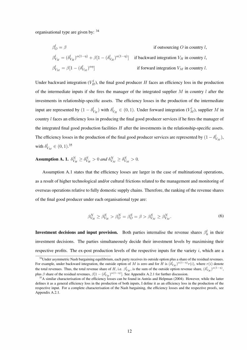
organisational type are given by: 34

βlO = β if outsourcing O in country l,

βlVH = (δlVH )α(1−η) + β[1− (δlVH )α(1−η)] if backward integration VH in country l,

βlVM = β[1− (δlVM )αη] if forward integration VM in country l.

Under backward integration (V lH ), the final good producer H faces an efficiency loss in the production

of the intermediate inputs if she fires the manager of the integrated supplier M in country l after the

investments in relationship-specific assets. The efficiency losses in the production of the intermediate

input are represented by (1 − δlVH ) with δlVH ∈ (0, 1). Under forward integration (V lM ), supplier M in

country l faces an efficiency loss in producing the final good producer services if he fires the manager of

the integrated final good production facilities H after the investments in the relationship-specific assets.

The efficiency losses in the production of the final good producer services are represented by (1− δlVM ),

with δlVM ∈ (0, 1).35

Assumption A. 1. δNVH ≥ δSVH

> 0 and δNVM ≥ δSVM

> 0.

Assumption A.1 states that the efficiency losses are larger in the case of multinational operations,

as a result of higher technological and/or cultural frictions related to the management and monitoring of

overseas operations relative to fully domestic supply chains. Therefore, the ranking of the revenue shares

of the final good producer under each organisational type are:

βNVH ≥ βSVH

> βNO = βSO = β > βSVM ≥ βNVM. (6)

Investment decisions and input provision. Both parties internalise the revenue shares βlk in their

investment decisions. The parties simultaneously decide their investment levels by maximising their

respective profits. The ex-post production levels of the respective inputs for the variety i, which are a34Under asymmetric Nash bargaining equilibrium, each party receives its outside option plus a share of the residual revenues.

For example, under backward integration, the outside option of M is zero and for H is (δlVH )α(1−η)r(i), where r(i) denotethe total revenues. Thus, the total revenue share of H , i.e. βlVH , is the sum of the outside option revenue share, (δlVH )α(1−η),plus β share of the residual revenues, β[1− (δlVH )α(1−η)]. See Appendix A.2.1 for further discussion.

35A similar characterisation of the efficiency losses can be found in Antras and Helpman (2004). However, while the latterdefines it as a general efficiency loss in the production of both inputs, I define it as an efficiency loss in the production of therespective input. For a complete characterisation of the Nash bargaining, the efficiency losses and the respective proofs, seeAppendix A.2.1.

12

function of the ex-ante investment decisions in the relationship-specific assets, are given by:36

xl,∗h,k(θ) =αβlkη

wNrl,∗k (θ),

xl,∗m,k(θ) =α(1− βlk)(1− η)

wlrl,∗k (θ),

(7)

with k = O, VH , VM , and the total revenues given by:

rl,∗k (θ) ≡ ασ−1θσ−1(γE)σQ1−σ

[(βlkwN

)η (1− βlkwl

)1−η]σ−1. (8)

Organisational choice. The final good producer faces a discrete set of possible organisational types.

Given the upfront payment, the final good producer chooses the organisational structure k, l that max-

imises the overall profits:

maxβlk

πlk(θ,Q, η) = θσ−1(γE)σQ1−σψlk(η)− wNf lk, (9)

with k = O, VH , VM , location l = N,S, and

ψlk(η) =

[1− α[βlkη + (1− βlk)(1− η)]

α1−σ

][(βlkwN

)η (1− βlkwl

)1−η]σ−1.

Assumption A. 2 (Ranking in organisational fixed costs).

fNO < fNVH < fSO + (1− λ)sr < fSVH + (1− λ)sr,

fNO < fNVM < fSO + (1− λ)sr < fSVM + (1− λ)sr,

where λ ∈ (0, 1) denotes the per-period survival rate to an exogenous ”death” shock.

I assume that the higher organisational complexity involved under integration, relative to the manage-

ment of two independent specialised firms, imposes additional managerial or governance costs (Coase,

1937; Williamson, 1979, 1985; Grossman and Helpman, 2002). Thus, the organisational fixed costs of

any type of integration in l cannot be smaller than the fixed costs of outsourcing in that same location, i.e.

f lO < f lVH and f lO < f lVM . Additionally, I assume that overseas operations require a larger management

structure relative to fully domestic supply chains. Both conditions together result in assumption A.2.

The optimisation program defined by (9) balances the two trade-off situations that the final good

producers face when they decide on the organisational structure of the supply chain from the discrete set36For a complete characterisation of the respective maximisation programs and proofs, see Appendix A.2.2.

13

of feasible types. From a property rights dimension, they can realise gains from integration by allocating

the property rights to the party that has the highest contribution to the relationship, but at the cost of facing

higher organisational fixed costs of integration due to the more complex structure of the organisation. At

the same time, from a location dimension, they can exploit the gains from offshoring that result from the

lower marginal costs of southern suppliers, but at the cost of higher fixed costs of offshore operations.

Sector classification and organisational types. In the case ofH-intensive sectors, i.e. when η ≥ ηc,37

backward integration minimises the hold up by transferring the property rights on all the assets to the

final good producer. However, I show in section 2.2 that for some final good producers, those gains are

surpassed by the higher fixed costs of integration.

In the case of M -intensive or component-intensive sectors, i.e. when η ≤ ηc, forward integra-

tion minimises the hold-up by transferring the property rights on all the assets to the manufacturer M .

However, those gains cannot compensate for the higher organisational fixed costs for some final good

producers.

In the case of the sectors with a balanced intensity between the two parties, i.e. when ηc < η < ηc,

outsourcing dominates any type of integration. Therefore, the only active dimension in the sourcing

decision is the location of the intermediate input supplier.

2.2 Perfect information steady-state.

The characterisation of the perfect information equilibrium is close to Antras and Helpman (2004). The

main departure comes from the possibility of forward integration as an additional organisational type.

This generalisation leads to the emergence of a third type of sector (balanced intensity) and a different

organisational structure of the component-intensive sectors compared to Antras and Helpman (2004).

H- and M -intensive sectors. In H-intensive sectors, forward integration is strictly dominated by the

other two organisational types. In M -intensive sectors, instead, backward integration is strictly domi-

nated by the other two organisational types. In both sectors, the equilibrium shows a sectoral structure

with four organisational types. The organisational structure in equilibrium for H- and M -intensive sec-

tors are similar, and they only differ in the type of integration that emerges. Thus, I characterise it in

general for both sectors, where V indicates VH for H-intensive sectors and VM for M -intensive sec-

tors.38

37For definition of the critical values ηc and ηc, see Appendix A.2.3.38See Appendix A.4 for proofs and explicit expressions for the productivity cutoffs.

14

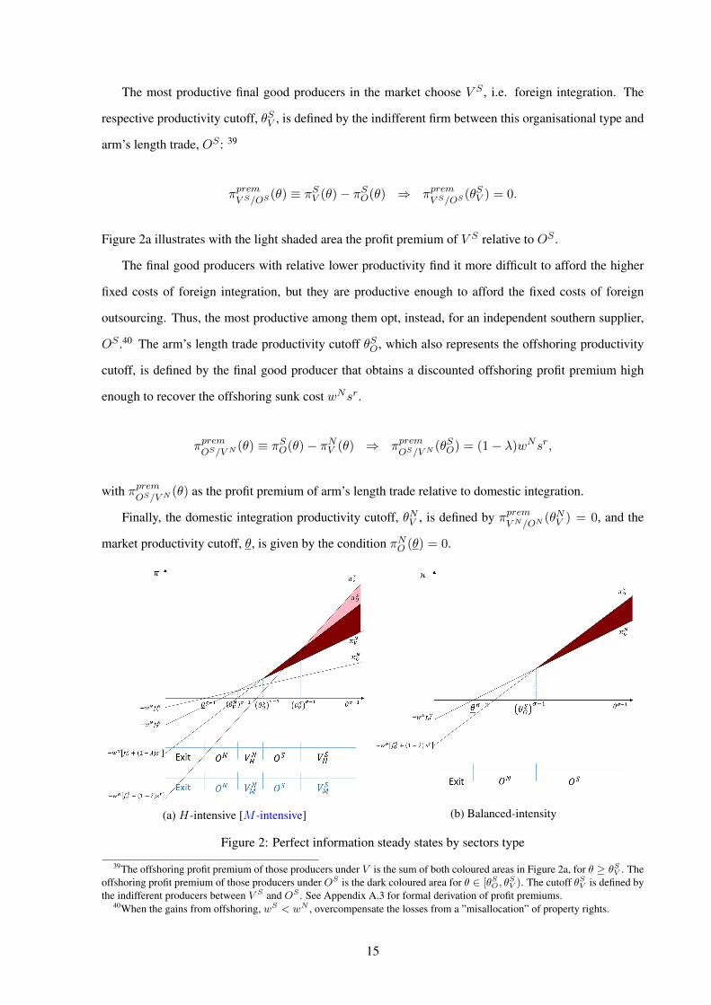
The most productive final good producers in the market choose V S , i.e. foreign integration. The

respective productivity cutoff, θSV , is defined by the indifferent firm between this organisational type and

arm’s length trade, OS : 39

πpremV S/OS

(θ) ≡ πSV (θ)− πSO(θ) ⇒ πpremV S/OS

(θSV ) = 0.

Figure 2a illustrates with the light shaded area the profit premium of V S relative to OS .

The final good producers with relative lower productivity find it more difficult to afford the higher

fixed costs of foreign integration, but they are productive enough to afford the fixed costs of foreign

outsourcing. Thus, the most productive among them opt, instead, for an independent southern supplier,

OS .40 The arm’s length trade productivity cutoff θSO, which also represents the offshoring productivity

cutoff, is defined by the final good producer that obtains a discounted offshoring profit premium high

enough to recover the offshoring sunk cost wNsr.

πpremOS/V N

(θ) ≡ πSO(θ)− πNV (θ) ⇒ πpremOS/V N

(θSO) = (1− λ)wNsr,

with πpremOS/V N

(θ) as the profit premium of arm’s length trade relative to domestic integration.

Finally, the domestic integration productivity cutoff, θNV , is defined by πpremV N/ON

(θNV ) = 0, and the

market productivity cutoff, θ, is given by the condition πNO (θ) = 0.

(a) H-intensive [M -intensive] (b) Balanced-intensity

Figure 2: Perfect information steady states by sectors type

39The offshoring profit premium of those producers under V is the sum of both coloured areas in Figure 2a, for θ ≥ θSV . Theoffshoring profit premium of those producers under OS is the dark coloured area for θ ∈ [θSO, θ

SV ). The cutoff θSV is defined by

the indifferent producers between V S and OS . See Appendix A.3 for formal derivation of profit premiums.40When the gains from offshoring, wS < wN , overcompensate the losses from a ”misallocation” of property rights.

15

Balanced-intensity sectors. Outsourcing strictly dominates any type of integration when the contribu-

tion of each party to the total output is relatively balanced. Therefore, only two organisational forms are

observed in these industries: domestic outsourcing and arm’s length trade.41 The sectoral organisational

structure under equilibrium is illustrated by Figure 2b.

The shaded area represents the offshoring profit premium for the final good producer with θ ≥ θSO.

The offshoring productivity cutoff, θSO, is defined by the final good producer that realises a discounted

offshoring profit premium high enough to recover the offshoring sunk cost.

πpremOS/ON

(θ) ≡ πSO(θ)− πNO (θ) ⇒ πpremOS/ON

(θSO) = (1− λ)wNsr.

Finally, the market productivity cutoff, θ, is defined by the condition πNO (θ) = 0.

The related-party trade database does not identify the type of integration (forward or backward).

However, the generalisation of the organisation-space allows me to overcome this data limitation and de-

rive predictions on organisational dynamics under institutional uncertainty that contemplates both types

of integration. Moreover, the analysis below remains robust to the situation where only one type of

integration is available (i.e. backward integration), as in Antras and Helpman (2004).42

3 Uncertainty in organisational fixed costs in South: model setup

A close reference to the characterisation of the Bayesian learning mechanism and the offshoring ex-

ploration decisions as a Markov decision process is Larch and Navarro (2021). The main difference is

that, by assuming incomplete contracts, my focus is on the organisational dynamics, i.e. in the dynamic

allocation of property rights across the value chain, while by assuming complete contracts, Larch and

Navarro (2021) center the attention in the location dimension of the sourcing decisions.43

3.1 Model setup and initial conditions.

The initial conditions are defined as the steady-state economy with non-tradable intermediate inputs

(n.t.i.). Offshoring strategies are initially not feasible for the northern final good producers due to weak

institutional fundamentals in South. The higher marginal costs in the North imply a higher price index,41See Appendix A.5 for proofs and explicit expressions for the productivity cutoffs in balanced-intensity sectors.42In Appendix E.2, I use data for US manufacturing sectors to analyse empirical evidence for the generalisation of the

organisational choice introduced in this section.43To avoid the emergence of multiple equilibria, I simplify the location dimension of the offshoring decision under in-

stitutional uncertainty. For a complete characterisation of the location dimension in offshoring decisions under institutionaluncertainty and its consequences in terms of specialisation of countries and welfare, see Larch and Navarro (2021).

16

P n.t.i., which translates into a lower competition intensity in the final good market.

Under n.t.i conditions, the most productive final good producers in the H-intensive [M -intensive]

sectors choose domestic backward [forward] integration, while the least productive producers opt instead

for domestic outsourcing. In the balanced-intensity sectors, they all choose domestic outsourcing.

I denote with ∗ the perfect information equilibrium variables. Comparing both steady states:44

• H[M ]-intensive sectors: θn.t.i. < θ∗ ; θN,n.t.iVH[M ]< θN,∗VH[M ]

; Pn.t.i. > P ∗ ; Qn.t.i. < Q∗,

• Balanced-intensity sectors: θn.t.i. < θ∗ ; Pn.t.i. > P ∗ ; Qn.t.i. < Q∗.

Institutional reform in South (t = 0). An institutional information shock (e.g. institutional reform)

takes place in the South in t = 0, but the weak credibility of the southern government produces that

northern final good producers do not fully believe in the fundamentals of the new institutional regime.

Thus, based on how credible the announcement of the southern government is, uncertainty emerges about

the per-period fixed costs for each organisational type that involves a southern supplier, i.e. fSO, fSVH, fSVM .

The final good producers’ prior beliefs at t = 0 about institutions in South post-reform are:

fSk ∼ Y (fSk ) with fSk ∈ [fSk , fSk ] and k = O, VH , VM , (10)

where Y (.) denotes the c.d.f. of the prior uncertainty.45

The organisational choice is modelled as a recursive Markov decision process where firms update

their beliefs through a Bayesian learning mechanism. Based on the priors, each final good producer

must decide whether to explore the offshoring potential or wait. If the final good producer chooses to

explore, she must pay a sunk cost for feasibility studies to set up a supply chain abroad, which consists

in the analysis of the possible offshoring strategies from the South. Thus, after paying the offshoring

sunk cost wNsr, she discovers the organisational fixed costs in the South for all the alternative types, i.e.

fSO, fSVH, fSVM . After she receives this information, she must choose the optimal organisational form.46

If, instead, she decides to wait, she does it by sourcing for one more period with a domestic supplier

under the previous organisational type k′N . At the beginning of the next period, she updates the prior

beliefs by observing the chosen organisational type of the final good producers that explored their off-44Appendix B characterises the n.t.i steady state for each type of sector. Appendix A.8 defines the price and aggregate

consumption indices under perfect information equilibrium for H- and M -intensive sectors, while Appendix A.7 defines themfor balanced-intensity sectors.

45For the moment, the only condition on the prior distribution is that it has a finite expected value. To avoid a taxonomy ofcases, I also assume that the true value is within the range of the distribution, i.e. fSk ∈ [fSk , f

Sk ].

46An important feature of the exploration activity is that it sets the final good producer in an absorbing state of the Markovprocess. After exploration, there is no remaining uncertainty to the final good producer.

17

shoring potential in the previous period. With this new information, she decides first whether to leave

the market or remain active. If she stays active, she decides whether to explore the offshoring potential

or wait one more additional period.

In the following sections, I introduce the information externalities and the learning mechanism. Then,

I characterise the exploration decisions of the initial explorers (t = 0) and the followers (t > 0). Figure

3 illustrates the timing of events of the recursive Markov decision process.

Figure 3: Timing of events - Uncertainty

3.1.1 Informational externalities and learning.

The learning mechanism involves the interaction of two states: the beliefs state and the physical state

(Larch and Navarro, 2021). The latter refers to the information externalities generated by the actions of

producers under offshoring. The first state defines how producers under domestic sourcing can update

their beliefs.

Physical state: information externalities. I define the maximum affordable fixed cost for a final good

producer under organisational type kS = OS , V SH , V

SM in period t as:

πpremkS/k′N ,t

(θ) = 0 ⇒ fSk (θ) =rNk (θ,Qt)

σwN

[(wN

wS

)(1−η)(σ−1)

− 1

]+ fNk′ , (11)

where k′N indicates V NH in the case of H-intensive sectors, V N

M for M -intensive, and ON for the indus-

tries with balanced intensity. It is easy to see that if fSk > fSk (θ) ∀kS , the final good producer θ does

18

not find it profitable to offshore under any type. Thus, after discovering her offshoring potential in the

South, she decides to remain sourcing domestically under the previous organisational type k′N .

I define θSk,t as the least productive final good producers doing offshoring under type k in t, and θSt as

the least productive producers that has explored the offshoring potential in t − 1. Thus, fSk,t ≡ fSk (θSk,t)

denotes the maximum affordable fixed cost under type k for the final good producers θSk,t in t, and

fSk,t ≡ fSk (θSk,t) indicates the maximum affordable fixed cost under type k for θSk,t in t.

Beliefs state: learning. The initial state of the beliefs is defined by the initial prior distributions in

equation (10), and they evolve according to the learning mechanism defined in (12). Intuitively, the

final good producers that have not explored their offshoring potential can learn by observing the other

producers’ behaviour (physical state). In particular, I assume that the final good producers can observe

the productivity θ of their competitors and the organisational type chosen by each of them.47

The posterior beliefs at the beginning of any period t > 0 for each k = O, VH , VM are given by:

fSk ∼

Y (fSk ) if fSk,t = fSk,t−1 = fSk ,

Y (fSk |fSk ≤ fSk,t) =Y (fSk |f

Sk ≤f

Sk,t−1)

Y (fSk,t|fSk ≤f

Sk,t−1)

if fSk,t = fSk,t < fSk,t−1,

fSk,t if fSk,t < fSk,t.

(12)

The first line indicates that the posterior beliefs for type k remain equal to the prior, when no final

good producer has yet offshored under that type. The second line indicates a truncation of the prior

uncertainty, exploiting the information that emerged from the new offshoring final good producers under

type k. As a result of applying Bayes rule, the distribution progressively truncates from the right, while

the lower bound of the prior remains constant.48 To simplify the notation, I removed the lower bound in

the condition of the distribution.

Finally, the third line indicates the moment in which the true value is revealed, and thus the uncer-

tainty distribution collapses to the maximum affordable fixed cost by the least productive producer that

offshores under type k. This takes place if, after exploring the offshoring potential in type k, at least one

final good producer returns to domestic sourcing. I discuss this further below.47Alternatively, if they can observe the total size of the final good market and the respective market shares of the competitors,

together with the chosen organisational type, they can infer the productivity level. In Appendix C.6, I define the learning processfor the situation in which the ownership structure is unobservable when offshoring, but they can still observe the location fromwhere the other final good producers are sourcing.

48For proofs of the derivation of the Bayesian updating process, see Appendix C.1. For a similar Bayesian learning processsee Rob (1991); Segura-Cayuela and Vilarrubia (2008); Larch and Navarro (2021)

19

3.1.2 Exploration decision of the offshoring potential.

The final good producer must decide whether to explore her offshoring potential under type k or wait by

sourcing domestically under its current organisational type.

Vk,t(θ; θSt ) = maxV ok,t(θ; θ

St );V w

k,t(θ; θSt ); for k = O, VH , VM ,

where θSt = θSO,t, θSVH ,t, θSVM ,t indicates the state of the sector in period t.

The value of exploring the offshoring potential for a final good producer θ under type kS = OS , V SH , V

SM

is given by the expected discounted profit premium of that type kS relative to the current domestic sourc-

ing organisational type k′N , net of the offshoring sunk cost wNsr:

V ok,t(θ; θ

St ) = Et

[max

0;∞∑τ=t

λτ−tπpremkS/k′N ,τ

(θ)

∣∣∣∣∣fSk ≤ fSk,t]− wNsr.

The final good producers, based on their posterior beliefs at t, can compute this expected value of off-

shoring for each alternative type, kS = OS , V SH , V

SM .

The value of waiting is defined as:

Vwk,t(θ; θSt ) = 0 + λEt[Vk,t+1(θ; θSt+1),

which is computed by the producers for each type kS = OS , V SH , V

SM , based on posterior beliefs at t.

The Bellman equation for each offshoring type takes the form:

Vk,t(θ; θSt ) = maxV ok,t(θ; θ

St );λEt[Vk,t+1(θ; θ

St+1)]

. (13)

Assumption A. 3. Information flow decreases in the upper bound:

∂[fSk,t − E(fSk |fSk ≤ fSk,t)]∂fSk,t

> 0.

Under assumption A.3, I show that the One-Step-Look-Ahead (OSLA) rule is the optimal policy

rule. In other words, in expectation at t, waiting for one period and exploring the offshoring potential in

the next period dominates waiting for any longer periods.49

Therefore, the Bellman equation becomes Vk,t(θ; θSt ) = maxV ok,t(θ; θ

St );V w,1

k,t (θ; θSt )

. From this

49This assumption implies that the information revealed is decreasing in time. See Appendix C.2 for proofs.

20

expression, I derive the trade-off function (14) for each offshoring type k = OS , V SH , V

SM :

Dk,t(θ; θSt , θSt+1) = V ok,t(θ; θ

St , θ

St+1)− V

w,1k,t (θ; θt, θt+1), (14)

where the first argument of the function refers to the final good producer θ taking the decision, the second

argument indicates the state of the system at the moment of the decision θSt , and the third argument

denotes the expected state of the system one period after, θSt+1.

When the value of offshoring is higher than the value of waiting, the final good producer finds it

profitable to explore the offshoring potential under type k in t. When it is negative, she finds it optimal to

wait for one period. When the trade-off function is zero, the final good producer is indifferent between

exploring and waiting. In the last case, I assume that she chooses to explore.

Dk,t(θ; θSt , θSt+1)

≥ 0 Explores offshoring potential in South under type k in t.

< 0 Waits one period sourcing under k′N .

After paying the offshoring sunk cost wNsr, the final good producer discovers the value of the fixed

costs in the South for all the offshoring organisational types. Therefore, she decides to explore her off-

shoring potential whenever the trade-off function is non-negative for at least one type k = OS , V SH , V

SM .50

Substituting the value of offshoring and the value of waiting into equation (14), I obtain:51

Dk,t(θ; θSt , θSt+1) = max

0;Et[π

premkS/kN ,t

(θ)∣∣∣fSk ≤ fSk,t]− wNsr

[1− λ

Y (fSk,t+1)

Y (fSk,t)

]. (15)

From this expression, I derive a first property of the equilibrium path. Consistently with Larch and

Navarro (2021), Lemma 1 shows that the exploration of the offshoring potential in the South is led by

the most productive final good producers in the market.

Lemma 1 (Sequential offshoring). The final good producers with higher productivity have an incentive

to explore the offshoring potential in earlier periods.

∂Dk,t(θ; θSt , θSt+1)

∂θ≥ 0.

Proof. See Appendix C.5.1.50After she receives that information, she may opt for a different organisational offshore structure than the type that triggered

the exploration decision. In section 3.2, I characterise the decisions for each sector.51See Appendix C.3 for derivation of equation (15).

21

Moreover, the trade-off function is strictly increasing in θ for those final good producers facing a real

trade-off, i.e. those with a positive value of offshoring.

Assumption A. 4. Dk,t=0(¯θ; ¯θ, ¯θ) > 0 for at least one k = O, VH , VM , where ¯θ refers to the most

productive final good producer in the market.

Assumption A.4 establishes that at least the most productive final good producer in the market,

denoted by ¯θ, finds it profitable at t = 0 to explore the offshoring potential for at least one organisational

type k = O, VH , VM . This is a necessary condition to trigger the sequential exploration of the offshoring

potential in South.52

3.2 Sectoral equilibrium paths.

I focus the analysis on the sectoral organisational dynamics, particularly on the vertical disintegration

patterns that result from an endogenous increase in competition intensity. Thence, I concentrate on

the characterisation of the equilibrium paths for the sectors where those patterns emerge, i.e. the M -

and H-intensive sectors. Given that both types of integration are strictly dominated by outsourcing in

balanced-intensity sectors, those dynamic patterns are absent in the sectoral equilibrium paths. Thus, I

characterise the latter in Appendix C.4.

Both H- and M -intensive sectors face similar equilibrium paths. The main difference is that the

integration type that emerges in the first case is backward, VH , while in the second case, it is forward,

VM . I characterise the equilibrium paths for both sectors together, where V refers to VH for aH-intensive

sector and VM for a M -intensive sector.

3.2.1 H- and M -intensive sectors: The trade-off function.

The final good producers may find it optimal to offshore by either arm’s length trade or integration. When

they must decide whether to explore their offshoring potential or wait, they compare the profits under

domestic integration with the expected profit under each of the two alternative offshoring types.53

The trade-off function is thus given by:

Dk,t(θ; θSt , θSt+1) = max

0;Et[πpremkS/V N ,t

(θ)∣∣∣fSk ≤ fSk,t]− wNsr

[1− λ

Y (fSk,t+1)

Y (fSk,t)

], (16)

52If the distribution G(θ) is unbounded on the right, i.e. ¯θ →∞, then the assumption A.4 holds for any distribution Y (fSk )with a finite expected value.

53In the case of H-intensive sectors V refers to VH . The other organisational types strictly dominate forward integration.Therefore, it is not considered a potentially profitable alternative. Instead, in M -intensive sectors, V indicates VM . The othertypes strictly dominate backward integration. Thus, it is not considered as a potentially profitable alternative.

22

with k = O, V . A final good producer with productivity θ explores the offshoring potential in period t

when Dk,t(θ; θSt , θSt+1) ≥ 0 for at least one k = OS , V S .

The offshoring exploration productivity cutoff, i.e. the least productive final good producer exploring

the offshoring potential, at any period t, is defined in Lemma 2.

Lemma 2 (Per-period offshoring exploration productivity cutoff). The offshoring exploration productiv-

ity cutoff in any period t, denoted as θSt+1, is given by:

θSt+1 = minθSO,t+1; θ

SV,t+1

,

with

θSO,t+1 = (γE)σ

1−σ Qt

wN

[E(fSO|fSO ≤ fSO,t)− fNV + sr

(1− λY (fSO,t+1)

Y (fSO,t)

)]ψSO(η)− ψNV (η)

1

σ−1

,

θSV,t+1 = (γE)σ

1−σ Qt

wN

[E(fSV |fSV ≤ fSV,t)− fNV + sr

(1− λY (fSV,t+1)

Y (fSV,t)

)]ψSV (η)− ψNV (η)

1

σ−1

.

Proof. θSO,t+1 and θSV,t+1 are defined by the fixed points:

DV,t(θV,t+1; θSt , θ

St+1) = 0⇒ Et

[πpremV S/V N ,t

(θV,t+1)∣∣∣fSV ≤ fSV,t] = wNsr

[1− λ

Y (fSV,t+1)

Y (fSV,t)

],

DO,t(θO,t+1; θSt , θ

St+1) = 0⇒ Et

[πpremOS/V N ,t

(θO,t+1)∣∣∣fSO ≤ fSO,t] = wNsr

[1− λ

Y (fSO,t+1)

Y (fSO,t)

].

See Appendix C.5.2.

Organisational choice after exploration. After paying the offshoring sunk cost wNsr, the producer

receives information on the true values fSO, fSVH, fSVM . Therefore, she chooses the organisational type that

maximises her profits, independently of the type k that triggered the exploring decision.

The organisational decision after exploration is as follows: After paying wNsr in period t, the final

good producer discovers the true values of fSO , fSVH and fSVM , and she must choose an organisational type.

The final good producer with productivity θ chooses foreign integration, V S , when:

πpremV S/OS ,t

(θ) =πSV,t(θ)− πSO,t(θ) ≥ 0.

23

She chooses arm’s length trade, OS , when:

πpremOS/V N ,t

(θ) =πSO,t(θ)− πNV,t(θ) ≥ 0 and πpremV S/OS ,t

(θ) < 0.

Otherwise, she remains under domestic integration.

Lemma 3 (Foreign integraton productivity cutoff). The foreign integration productivity cutoff at the end

of period t, θSV,t+1 , i.e. the least productive final good producer that has chosen V S after paying the

sunk cost in period t, is given by:

θSV,t+1 = maxθSt+1; θ

S,•V,t+1

, (17)

with

πpremV S/OS ,t

(θS,•V,t+1) = 0 ⇒ θS,•V,t+1 = (γE)σ

1−σ Qt

[wN

[fSV − fSO

]ψSV (η)− ψSO(η)

] 1σ−1

. (18)

Proof. See Appendix C.5.3.

3.2.2 H- and M -intensive sectors: Long-run properties of the trade-off function.

Lemma 4 (Convergence of offshoring productivity cutoff). The sector converges asymptotically to the

perfect information equilibrium, θStt→∞−−−→ θS,∗ = θS,∗O , when:

Case I: fSO = fSO ⇒ fSO,∞ = fSO,

Case II: fSO + (1− λ)sr < fSO.

Hysteresis takes places, i.e. convergence leads to some ”excess” of offshoring , when:

Case III: fSO + (1− λ)sr = fSO ⇒ θStt→∞−−−→ θS,¬rO ,

Case IV: fSO + (1− λ)sr > fSO > fSO ⇒ θStt→∞−−−→ θSO,∞,

with θS,∗O > θSO,∞ > θS,¬rO , and θS,¬rO denoting the case where the marginal firms obtain zero per period

offshoring profit premium by doing arm’s length trade, i.e. firms who cannot recover wNsr.

Proof. See Appendix C.5.4.

I define t as the earliest period in which: θSt+1≤ θS,•V,t+1, i.e. for t > t, the new producers exploring

the offshoring potential in South choose foreign outsourcing after the exploration decision. Figure 4a

illustrates the cases characterised in Lemma 4. Depending on the optimistic level of the priors, t may

24

take place right in the first period, i.e. t = 0, or in any finite period after the initial one. Under Case II, t

necessarily takes place before the period in which the convergence stops. This is a natural consequence

of the sequential offshoring process.

(a) Offshoring productivity cutoff (b) Productivity cutoffs

Figure 4: H- and M -intensive sectors. Equilibrium paths

3.2.3 H- and M -intensive sectors: Competition effect and the disintegration dynamics.

As more firms explore their offshoring potential, the offshoring productivity cutoff converges to the

long-run steady states defined by Cases I to IV in Lemma 4. The lower prices charged by the final good

producers under offshoring reduce the price index and increases the aggregate consumption index in the

final good markets. The price index and the aggregate consumption index converge to their respective

long-run steady states defined by Cases I to IV, as shown by Lemma 5.

Lemma 5 (Price index effect of sequential offshoring). As the offshoring productivity cutoff converges

to the steady state (Lemma 4), the price index in the final good market reduces:

Cases I and II: Pt P ∗ if θSt θS,∗,

Case III: Pt P¬r if θSt θS,¬r,

Case IV: Pt P∞ ∈ (P ∗;P¬r) if θSt θS∞ ∈ (θS,¬r; θS,∗).

Proof. See Appendix C.5.5.

Lemma 6 (Convergence of market productivity cutoff). As the offshoring productivity cutoff converges

to the steady state (Lemma 4), the price index in the final good market reduces (Lemma 5), and the

25

market productivity cutoff increases:

Cases I and II: θt θ∗ if θSt θS,∗,

Case III: θt θ¬r if θSt θS,¬r,

Case IV: θt θ∞ ∈ (θ∗; θ¬r) if θSt θS∞ ∈ (θS,¬r; θS,∗).

Proof. See Appendix C.5.6.

From Lemma 6, it is possible to see that the decreasing price index intensifies the competition in

final good market, and sequentially pushes the least productive final good producers out of the market.

As Pt P ∗, the market productivity cutoff θt θ∗.

Proposition 1 (First channel of competition effect on vertical disintegration). As the offshoring produc-

tivity cutoff converges to the steady state (Lemma 4), the price index in the final good market reduces

(Lemma 5), and:

(a) the least productive final good producers under domestic integration sequentially disintegrate the

supply chains to domestic outsourcing:

Cases I and II: θNV,t θN,∗V if θSt θS,∗,

Case III: θNV,t θN,¬rV if θSt θS,¬r,

Case IV: θNV,t θNV,∞ ∈ (θN,∗V ; θN,¬rV ) if θSt θS∞ ∈ (θS,¬r; θS,∗).

(b) starting from t, the least productive final good producers under foreign integration sequentially

disintegrate the supply chains to foreign outsourcing:

Cases I and II: θSV,t θS,∗V if θSt θS,∗,

Case III: θSV,t θS,¬rV if θSt θS,¬r,

Case IV: θSV,t θSV,∞ ∈ (θS,∗V ; θS,¬rV ) if θSt θS∞ ∈ (θS,¬r; θS,∗).

Proof. See Appendix C.5.7.

Figure 4b illustrates the equilibrium paths of the productivity cutoffs for Case I (solid line) and Case

III (dashed line). Any path between I and III represents Case IV. For simplicity, I will refer from now on

to either of the long-run steady states as the perfect information steady-state.54

54As shown in Lemma 4, some steady states differ from the perfect information equilibrium (hysteresis). Nevertheless, for

26

Effects on offshoring firms: regime change and sequential disintegration. Proposition 1 (b) shows

that the least final good productive producers under foreign integration sequentially shift to foreign out-

sourcing, as the competition in the final goods market intensifies. For t ≥ t, as Pt P ∗, the foreign

integration productivity cutoff converges from below to the perfect information steady state: θSV,t θS,∗V .

The least productive of the early offshoring final good producers have chosen V S as a temporal

organisational type. As the competition intensifies, they find it optimal to vertically disintegrate and

switch to arm’s length trade.55 This represents a non-monotonic behaviour of the foreign integration

productivity cutoff over time. It manifests itself as a regime change or a reorganisation of the supply

chains of the least productive final good producers that have initially chosen foreign integration.56

Effects on middle size firms: sequential disintegration of domestic supply chains. Proposition 1

(a) shows that the least productive producers under domestic integration sequentially disintegrate the

supply chain to domestic outsourcing. As before, due to the effect of the increasing competition on

the revenues, some domestically integrated final good producers discover that the gains from integration

can no longer compensate for the higher managerial or governance costs. Thus, they sequentially shift

towards independent northern suppliers (domestic outsourcing).

4 Empirical model: Competition effect in North-South model

I test the theoretical prediction characterised by Proposition 1: the first channel of competition effect

on vertical disintegration. In particular, I focus on the organisational dynamics of the offshoring final

good producers.57 To that aim, I use US manufacturing sector-level data for the period 2002-2016. I

describe the data in section 4.1, and I follow with stylised facts in section 4.2. In sections 4.3.1 to

4.3.5, I introduce a set of reduced-form empirical models that capture different features of the sectoral

organisational dynamics. Finally, in section 4.3.6, I aggregate the firm-level predictions of the theoretical

model to sector-level consistent organisational dynamics, and I derive a structural two-stage empirical

simplicity, I refer as ”convergence to perfect information equilibrium” to any of those cases. For further discussions on thewelfare consequences of each steady-state, see Larch and Navarro (2021).

55For simplicity, I assume that there is zero cost of reorganisation of the supply chain when they switch from foreign inte-gration to foreign outsourcing. The introduction of a cost of disintegration would simply shift upwards the productivity level inthe conditions that define the period t.

56The increase in competition intensity in the final good market shrinks the total revenues for all the active final goodproducers. It diminishes the outside options at the bargaining stage of the final good producers under integration. Thus, itaffects proportionally more to those final good producers under integration. Therefore, a subset of the final good producersunder V S observes that the gains from integration cannot compensate for the higher managerial costs of that organisationaltype. Thus, they sequentially shift the regime from V S towards OS .

57In other words, I test for the effects characterised in part (b) of Proposition 1. The available data does not allow to test forthe vertical disintegration dynamics on domestic supply chains.

27

model that identifies the mechanism of the competition effect characterised Proposition 1.

4.1 Data.

The main datasets are the Related-Trade Party dataset and the manufacturing survey, both from the US

Census Bureau, and the supplementary import table before redefinitions of the input-output matrix from

the Bureau of Economic Analysis (BEA).

I use imports data for the period 2002-2016 from the Related-Trade Party dataset, provided by the

US Census Bureau.58 The data covers US manufacturing sectors reported at NAICS 6 digits, classified

according to the supplier’s (i.e. exporter’s) activity. The data allows for the distinction between imports

of US firms from a related party (intra-firm trade) and a non-related party (independent suppliers). The

sector-level aggregation constitutes the main drawback of the data for a complete structural estimation

of the model’s predictions. For that reason, I aggregate the firm-level model’s predictions and derive the

respective sectoral organisational equilibrium dynamics.

A second limitation of the data refers to the lack of distinction between forward and backward inte-

gration in imports flows. Instead, it identifies whether the parties are related (in either way) or indepen-

dent. Nevertheless, the generalisation of the organisational space in the theoretical model to both types

of integration allows me to overcome this limitation in the data. Thus, the model’s prediction test does

not require the distinction between forward and backward integration.

A third limitation comes from the classification of imports at the supplier sector, while the model’s

predictions are defined at the final good producer sector. Thus, to reclassify the data from supplier to

final good producer sectors, I use import matrix before redefinitions 2012 of the input-output matrix

provided by the BEA. I identify the final good producer sectors by the user manufacturing industries in

the matrix, while the supplier sector is linked to the manufacturing industries of the imported commodity

in the matrix. Both are classified by BEA code. After reclassification of the manufacturing survey and

the related-trade party datasets to BEA code, I merge both datasets to the matrix. Thus, I obtain a sample

that consists of 139 final good sectors, 160 supplier sectors, and 173 foreign countries.

Considering that the main predictions of the theoretical model are related to the organisational dy-

namics of the final good producer sectors, I aggregate the m (i.e. supplier) dimension in the data and

identify the mean supplier sector features at the final good producer level.

Regarding the imports data, I transform it to obtain the imports at final good producer sector j level.

To that aim, I build a measure based on the BEA matrix that captures the share of each final good sector58For the period 2005-2016, the data comes directly from the Census Bureau. For the years 2002-2004, I use the data of the

Census Bureau provided in Antras (2015).

28

j in the imports of each input m sector. It is denoted as HshrMm,j . Using these shares, I distribute the

imports of each input m through each final good sector j and aggregate them at the j level. Thus, I

compute the total imports and the intra-firm imports of each sector j from each sourcing location. The

manufacturing survey provides data on total sales of the final good producer sector j.59 Combining this

data with the imports data at sector j level, I compute the offshoring share and the intra-firm intensity of

each final good sector j.60 In section 4.3, I discuss the construction of the main variables.

I use the ”liberal” criteria of Rauch (1999)’s classification of commodities. I define a measure that

takes the value 0 if Rauch’s category is ”w”, 0.5 if ”r”, and 1 if ”d”.61 After reclassification to BEA

codes, I obtain a continuous differentiation index in [0, 1], which increases in the differentiation of the

sector. I merge this data with the input-output matrix and obtain a differentiation index for j and m sides

of the relationship. Thus, I obtain a weighted mean supplier differentiation index at the sector j level.

The elasticity of substitution of the final good markets comes from Broda and Weinstein (2006), and

the data on bilateral tariffs comes from the World Integrated Trade Solutions (WITS). I reclassify these

datasets to BEA codes and compute the respective mean values for each sector j.

Finally, using a factor analysis approach (FA), I build a measure for H-intensity of the final good

sector, ηj , which is defined by the first factor from a factor analysis of the determinants of theH-intensity.

To that aim, I build on the works of Yeaple (2006); Nunn (2007); Nunn and Trefler (2013) and Antras

(2015).62 The data used for that purpose comes from the manufacturing survey of the Census Bureau

and the Business R&D and Innovation Survey (BRDIS) survey of the National Center for Science and

Engineering Statistics (NCSES) of the National Science Foundation.

4.2 Stylised facts.

Figure 5a shows a positive trend in US total imports for differentiated and non-differentiated supplier’s

sectors.63 The positive trend in total imports and the negative trend in the share of intra-firm imports

of the differentiated sectors shown by Figure 5 are consistent with the sectoral equilibrium path char-

acterised in Section 3.2. The model’s prediction states that the sequential offshoring equilibrium path

increases the competition intensity in the final good markets, and thus it eventually leads to a sequential59Additionally, the manufacturing survey data is used to compute the measures of the determinants of the component-

intensity of the sector j in the static empirical model. For further discussion on the data and identification of the static empiricalmodels, see appendices E.1 and E.2.

60The offshoring share is the total imports of sector j over the total sales of the sector. Instead, the intra-firm intensity isdefined as the total intra-firm imports of sector j over the total sales of the sector. Additionally, I compute for the reduced-formmodel the intra-firm share, which refers to the intra-firm imports over the total imports of the sector j.

61The catergories are: i) good traded on an organised exchange (w), ii) reference priced (r), and iii) differentiated (d).62Main measures are: Capital intensity, Machinery intensity, R&D intensity, Advertising intensity. See Appendix E.2.63The vertical lines indicate the global financial crisis.

29

vertical disintegration of the offshoring firms. Additionally, Figure 5b shows an increasing participation

of independent suppliers in US imports, in particular in the differentiated supplier’s industries. 64

(a) Total imports, millions USD. (b) Intra-firm import share.

Figure 5: US imports by type of input m sector (differentiated and non-differentiated).

Figure 6 illustrates the predicted sectoral dynamic path and highlights the main features of the first

channel of the competition effect on vertical disintegration. The sequential reduction in the offshoring

productivity cutoff (red solid line) translates to a progressive increase in the competition intensity in the

final goods market (i.e. reduction of the sector’s price index). Among offshoring firms, it leads to a

sequential vertical disintegration of the least productive final good producers under foreign integration

(blue dashed line), which begins in period t.65

4.3 Identification of the empirical models and estimation results.

I test for the predictions of Proposition 1, i.e. the first channel of competition effect on vertical disinte-

gration, in particular those related to the organisational dynamics of offshoring firms. In sections 4.3.1 to

4.3.5, I introduce a set of reduced-form models that show evidence consistent with different features of

the organisational dynamics characterised by Proposition 1. Sections 4.3.1 and 4.3.2 present the models

in a two-country setup, where I aggregate the foreign sourcing locations. Sections 4.3.3 and 4.3.4 exploit

the variation that comes from the country dimension. Section 4.3.5 disentangles the bilateral and global

effects of the offshoring activity on the vertical disintegration of supply chains.

Finally, in section 4.3.6, I introduce main specification. It refers to a two-stage structural empirical

model that identifies the mechanism of the first channel of the competition effect on vertical disintegra-64This pattern is also consistent with the increasing offshoring activity of US firms shown in Feenstra (1998) for an earlier

period. There is a more stable behaviour pattern in the sense that the trend shows a consistently negative trend all over theperiod, except during the financial crisis. During the crisis, it showed a small increase, but it returned quickly to the decreasingtrend. It is consistent with a progressive vertical disintegration of the offshoring firms (Feenstra, 1998).

65The green dotted lines illustrate the effect of the increasing competition intensity in the domestic supply chains.

30

Figure 6: First channel of competition effect: increase in offshoring activity

tion, as characterised by Proposition 1.

4.3.1 Reduced form model: First channel of competition effect in a two-countries setup.

Following the North-South setup, I aggregate the country dimension to one offshoring location. Given

the non-linear nature of the model, I define a fractional logit model given by:

E[IFshrj,t

∣∣∣x] =exp(x′

j,tρ)

1 + exp(x′j,tρ)

with x′j,tρ =ρ1 ln(offshr shrj,t) + other controls + ρt, (19)

where IFshrj,t indicates the global intra-firm import share of sector j in year t, and offshr shrj,t measures

the offshoring share of sector j in period t. Among the other controls, I include a set of sector-level

variables that account for the relevant dimensions identified by the theoretical model.66 The control

variables are: the elasticity of substitution of the final good sectors, from Broda and Weinstein (2006)

(sigmaj), the degree of differentiation of the mean supplier sector relative to sector j (M diffj),67 and

the differentiation degree of the final good producer sector (H diffj). The model also includes year fixed

effects (ρt). Finally, the observations are weighted by the relevance of final good sector j in imports of66These control variables also account for the sector-level determinants of the organisational choices identified by the previ-

ous empirical literature. See Yeaple (2006); Nunn (2007); Nunn and Trefler (2013); Antras (2015).67This measure is similar to the contract dependence index from Nunn (2007). I describe below the construction of the

weighted mean measure of the differentiation index.

31

supplier sector m, i.e. HshrMm,j .

Definition of the main variables. From the manufacturing survey, I obtain the final good sector total

sales in year t, total salesj,t, while the data on total imports and intra-firm imports at the input sector

level in year t, total impm,t and IF impm,t, comes from the related-party trade dataset.68

The variable IFshrj,t is defined as:

IFshrj,t =∑m

IFshrm,t ×MshrHm,j with IFshrm,t =IF impm,t

total impm,t, (20)

and the offshoring share, offshr shrj,t, is:

offshr shrj,t =total impj,ttotal salesj,t

with total impj,t =∑m

total impm,t × HshrMm,j . (21)

The variable offshr shrj,t captures the intensity of offshoring activity in sector j, which is related to the

red solid line in Figure 6. The model predicts a negative coefficient ρ1: higher offshoring activity in

sector j (decreasing red solid line) leads to lower intra-firm import share (increasing blue dashed line).

The differentiation index for the mean supplier of sector j is M diffj =∑

m M diffm ×MshrHm,j .

Results. Column (1) of Table 1 reports the estimated coefficients and average marginal effects of the

model in equation (19). Column (2), instead, introduces the offshoring share in levels.69 The empirical

evidence is consistent with the theoretical predictions of Proposition 1: as the offshoring activity in the

sector increases, the intra-firm import share decreases. The latter is consistent with a vertical disintegra-

tion of the offshore supply chains.

However, the results may also capture a situation where the intra-firm import share increases but

offshoring final good producers do not vertically disintegrate their supply chains. In Figure 6, it would

be represented by a decreasing red solid line, while the blue dashed line remains horizontal from t on. To

account for the latter concern, I introduce a complementary reduced-form model in section 4.3.2, which

is able to account for this potential situation.68Total imports is defined as the sum of related-party imports plus non-related party imports. The non-classified imports are

removed from the sample.69See Table 10 in Appendix E.3.2 for complete table. Table 11 in Appendix E.3.2 reports the results of models that control

for sector j fixed effects. The supportive evidence vanishes in the latter case.

32

Table 1: Competition effect: coefficients and average marginal effects.

(1) (2) (3)IFshrj,t IFshrj,t IFintj,t

+ ++ + ++ + ++ln(offshr shrj,t) -0.180∗∗ -0.0381∗∗∗

(0.0768) (0.0139)

offshr shrj,t -2.356∗ -0.506∗ 11.69∗∗∗ 0.279∗∗∗

(1.427) (0.289) (1.319) (0.0389)

offshr shr2j,t -6.006∗∗∗ -0.143∗∗∗

(1.268) (0.0331)FEs t t t t t t

Observations 2039 2039 2039 2039 2039 2039Other controls: H diffj , M diffj , ln(sigmaj), η(FAj). Coefficients (+) and average marginal effects (++).

Standard errors in parentheses. Cluster s.e. at sector j. ∗ p < 0.10, ∗∗ p < 0.05, ∗∗∗ p < 0.01

4.3.2 Reduced form model: Intra-firm intensity.

I define IFintj,t as the intra-firm intensity in the sector j in period t, which is given by:

IFintj,t =IF impj,t

tot salesj,twith IF impj,t =

∑m

imp relm,t × HshrMm,j (22)

The dynamics illustrated in Figure 6 show that the intra-firm intensity exhibits a non-monotonic be-

haviour over time. Until period t, the intra-firm intensity increases as the offshoring activity in the sector

progressively increases (sequential offshoring). From that moment on, a further increase in offshoring

activity leads to a progressive reduction in the intra-firm intensity. Thus, considering the U-shaped rela-

tionship predicted by the theory, the empirical model specifies a quadratic relation between the offshoring

share and the intra-firm intensity. I define it as a fractional logit model, which is given by:

E[IFintj,t

∣∣∣x] =exp(x′

j,tρ)

1 + exp(x′j,tρ)

with x′j,tρ = ρ1offshr shrj,t + ρ2offshr shr2j,t + other controls + ρt,

(23)

Results. Column (3) of Table 1 reports the results of model in (23).70 The inverted U-shape of the

effect of the offshoring share on the intra-firm intensity provides evidence consistent with the predictions

of the model: once the sector has reached a sufficiently extensive offshoring activity, characterised by t,

further increase in the offshoring share induces a vertical disintegration of the offshore supply chains.70See 10 in Appendix E.3.2 for report of full table. Table 11 in Appendix E.3.2 reports the results of models that control for

sector j fixed effects. The results remain robust.

33

4.3.3 Reduced form model: Competition effect at bilateral levels.

I exploit now the variation in the country dimension. I estimate the effects of the global offshoring

activity of sector j in the bilateral intra-firm import shares.

The empirical model is given by:

E[IFshrl,j,t

∣∣∣x] =exp(x′

l,j,tρ)

1 + exp(x′l,j,tρ)

with x′l,j,tρ =ρ1 ln(offshr shrj,t) + other controls + ρl + ρt,

(24)

where IFshrl,j,t indicates the bilateral intra-firm import share of sector j from country l in year t, and

offshr shrj,t refers to the offshoring share of sector j in period t from all sourcing locations. From the

theory, the increase in the offshoring activity in any country l affects the organisation of supply chains

in all sourcing locations, through its impact on the price index in the final good market. Therefore, the

bilateral intra-firm import share of sector j is affected by the global offshoring activity of sector j.

As before, the other controls include: the elasticity of substitution from Broda and Weinstein (2006);

the degree of differentiation of the mean supplier industry, M diff, which is defined by equation (19);

the H differentiation level (H diff); and ln(1 + tariffsl,j,t), where tariffsl,j,t denotes the weighted mean

of tariffs in inputs imported by sector j in year t from country l. For the definition of the variables,

see Appendix E.3.2. The model includes country (ρl) and year (ρt) fixed effects. The observations are

weighted by the relevance of the final good sector j in supplier sector m’s imports, i.e. HshrMm,j .

Table 2: Competition effect: average marginal effects.

(1) (2) (3) (4) (5) (6)IFshrl,j,t IFshrl,j,t IFshrl,j,t IFshrl,j,t IFintl,j,t IFintl,j,t

ln(offshr shrj,t) -0.00598∗∗ -0.00756∗∗∗

(0.00264) (0.00244)

offshr shrj,t -0.0280 -0.0417 0.0109∗∗∗ 0.0104∗∗∗

(0.0333) (0.0304) (0.00117) (0.00107)

offshr shr2j,t -0.00494∗∗∗ -0.00473∗∗∗

(0.00116) (0.00111)FEs l , t lt l , t lt l , t lt

Observations 60979 60979 60979 60979 60979 60979Other controls: ln(1 + tariffl,j,t), H diffj , M diffj , ln(sigmaj), η(FAj). Average marginal effects.

Standard errors in parentheses. Cluster s.e. at sector j. ∗ p < 0.10, ∗∗ p < 0.05, ∗∗∗ p < 0.01

Results. Columns (1) and (2) of Table 2 show the estimation results of the model in equation (24). The

empirical models provide supportive evidence for the competition effect predicted by Proposition 1: as

34

the global offshoring activity in sector j increases, the bilateral intra-firm import share decreases. The

latter is consistent with a progressive vertical disintegration of the supply chains. The effect vanishes

when the offshoring share is introduced in levels (see columns (3) and (4)).71

4.3.4 Reduced form model: Intra-firm intensity.

I analyse the effect of the global offshoring activity in the bilateral intra-firm intensity. The empirical

model is given by:72

E[IFintl,j,t

∣∣∣x] =exp(x′

l,j,tρ)

1 + exp(x′l,j,tρ)

with x′l,j,tρ = ρ1offshr shrj,t + ρ2offshr shr2j,t + other controls + ρl + ρt,

(25)

Results. The results of model in equation (25) are reported in columns (5) and (6) of Table 2. They

provide evidence in favour of the quadratic relationship between the global offshoring share and the

bilateral intra-firm intensity, consistent with the sectoral dynamics illustrated in Figure 6.73

4.3.5 Reduced form models: Bilateral and global effects.

From theory, the characterisation of the mechanism of the competition effect through the price index

implies that the global offshoring activity of the sector affects the bilateral intra-firm import share (and

the bilateral intra-firm intensity). The alternative would be an effect limited to the bilateral relationships,

without global effects. Thus, the latter would provide evidence that the impact of the offshoring activity

is not channelled through the sector’s price index in the final good market.

To that aim, I disentangle the bilateral offshoring share and the global offshoring share of the sector

j, and test for their impact on the bilateral intra-firm import share (and the bilateral intra-firm intensity).

The empirical models are given by:

E[IFshrl,j,t

∣∣∣x] =exp(x′

l,j,tρ)

1 + exp(x′l,j,tρ)

; E[IFintl,j,t

∣∣∣x] =exp(x′

l,j,tρ)

1 + exp(x′l,j,tρ)

, (26)

with

x′l,j,tρ = ρ1 ln(offshr shrl,j,t) + ρ2 ln(offshr shr¬l,j,t) + other controls + ρl + ρt,

where ¬l indicates the aggregation of all the countries excluding l.71See Table 12 in Appendix E.3.2 for report of the full table. Table 13 in Appendix E.3.2 reports the results for the models

with sector j fixed effects. As before, the evidence is not consistent with the theoretical predictions in the latter case.72For the definition of the variables, see Appendix E.3.2.73Appendix E.3.2: Table 12 in reports full table, and Table 13 reports models with sector fixed effects. Results remain robust.

35

Table 3: Competition effect: bilateral and global effects.

(1) (2) (3) (4)IFshrl,j,t IFintl,j,t IFshrl,j,t IFintl,j,t

+ ++ + ++ + ++ + ++ln(offshr shrl,j,t) 0.144∗∗∗ 0.0111∗∗∗ 1.151∗∗∗ 0.00142∗∗∗ 0.158∗∗∗ 0.0117∗∗∗ 1.105∗∗∗ 0.00135∗∗∗

(0.0276) (0.00237) (0.0327) (0.0000622) (0.0208) (0.00184) (0.0211) (0.0000464)

ln(offshr shr¬l,j,t) -0.123∗∗∗ -0.00951∗∗∗ -0.0636∗∗∗ -0.0000787∗∗∗ -0.155∗∗∗ -0.0115∗∗∗ -0.0916∗∗∗ -0.000112∗∗∗

(0.0278) (0.00201) (0.0206) (0.0000259) (0.0282) (0.00191) (0.0185) (0.0000210)FEs l , t l , t lt lt l , t l , t lt lt

Observations 60978 60978 60978 60978 60978 60978 60978 60978Other controls: H diffj , M diffj , ln(1 + tariffl,j,t), ln(sigmaj), η(FA)j . Coefficients (+) and average marginal effects (++).

Standard errors in parentheses. Cluster s.e. at sector j. ∗ p < 0.10, ∗∗ p < 0.05, ∗∗∗ p < 0.01

Results. Table 3 shows that the effect of the offshoring activity on the vertical disintegration of the

supply chains is driven by the global offshoring activity. This result is consistent with an effect channelled

through the changes in sector’s price index.

4.3.6 Empirical model: Identification of the competition effect mechanism.

I introduce a two-stage model that identifies the mechanism of the first channel of the competition effect

on vertical disintegration through the price index in the final good markets, as characterised by Proposi-

tion 1. For the derivation of the respective regressions, see Appendix E.3.3.

In a first-stage regression, I estimate the effect of the offshoring share in the sector’s price index. To

that aim, I derive the following log-linear model:

ln(Pj,t) = b0 + b1 ln(offshr shrj,t) + other controls + bl + bt + uj,t. (27)

In a second-stage regression, I use the predicted value of ln(Pj,t) from the first stage and estimate

the effect on the intra-firm intensity. In other words, I use the predicted changes in the sector j’s price

index produced by changes in the sector’s offshoring share. Thus, the second-stage regression is defined

as a fractional logit model given by:

E[IFintl,j,t

∣∣∣x] =exp(x′

l,j,tρ)

1 + exp(x′l,j,tρ)

with x′l,j,tρ =ρ1 ln(Pj,t) + other controls + ρl + ρt. (28)

Results. The results are reported in Table 4.74 Regarding the first regression, the table shows that an

increase in the sectoral offshoring activity reduces the sector’s price index in the final good market. The

result is consistent with the intensification of the competition in the final good market due to a progressive

increase in the share of offshoring final good producers.74See full table of first stage regression in Table 14 in Appendix E.3.3.

36

The results of the second-stage regression provide supportive evidence for the vertical disintegration

consequences of the competition effect predicted by the theory. Reductions in the sector’s price index,

predicted by an increase in the sector offshoring activity, result in a lower intra-firm intensity in the

sector.

Table 4: Competition effect: Estimation in two stages.

Second stage: Coefficients reportedAgg. countries No aggregation of countries

(1) (2) (3)IFintj,t IFintl,j,t IFintl,j,t

ln(Pj,t) -35.43∗∗∗ -25.63∗∗∗ -25.74∗∗∗

(1.814) (1.598) (1.545)

ln(1 + tariffl,j,t) 51.88∗∗ 61.78∗∗∗

(22.253) (17.724)

H diffj 2.486∗∗∗ 2.905∗∗∗ 2.982∗∗∗

(0.573) (0.533) (0.514)

M diffj -0.164 2.855∗∗∗ 2.755∗∗∗

(0.363) (0.524) (0.482)

ln(sigmaj) 2.583∗∗∗ 2.046∗∗∗ 2.063∗∗∗

(0.195) (0.16) (0.158)

η(FA)j 0.191∗ -0.362∗∗ -0.345∗∗

(0.101) (0.159) (0.146)FEs t l , t lt

First stage: Main coefficients(1) (2) (3)

ln(Pj,t) ln(Pj,t) ln(Pj,t)

ln(offshr shrj,t) -0.0312∗∗∗ -0.0350∗∗∗ -0.0352∗∗∗

(0.00869) (0.00959) (0.00979)FEs t l , t ltR2 0.292 0.297 0.309Adjusted R2 0.285 0.294 0.282Second stage: Bootstrapped s.e. (1000 rep). Coefficients reported.

All stages: Cluster s.e. at sector j. Standard errors in parentheses.∗ p < 0.10, ∗∗ p < 0.05, ∗∗∗ p < 0.01

To sum up, the model shows that an increase in the offshoring activity impacts on a reduction of the

sector’s price index, which translates into a more intensive competition in the final good markets. The

theory predicts that the latter leads to a progressive vertical disintegration of the offshore supply chains,

supported by the findings above.

37

5 Multiple countries

In a world with multiple countries, the effect of the offshoring decisions on the price index, and thence

on the sector’s organisational structure, may not be independent of the location of the suppliers. Thus,

it may also come from the relocation of offshore suppliers across foreign countries. Therefore, I extend

the model to multiple countries. The main goal is to characterise the relocation dynamics of offshore

suppliers after an institutional reform in one low-wage foreign country (the East) takes place. Under

such conditions, I study the consequences of the competition effect on the organisational dynamics.75

I define a world economy with three countries: East (E), North (N ) and South (S). The production

of the services xh and the final good varieties are still produced only in the North, but the intermediate

inputs xm can be supplied by manufacturers in any location.

Assumption A. 5. Wages are higher in the South than in the East, but institutional fundamentals are

better in South for each organisational type.

wE < wS < wN ; fSO < fSV < fEO < fEV with V = VH , VM .

I assume that East have lower marginal costs than South, but the institutional fundamentals are better

in South.76 In addition to Assumption A.2, the Assumption A.5 defines the marginal costs differences

and the institutional fundamental conditions in foreign countries. However, the ranking on institutional

fundamentals is unknown to the final good producers when I introduce uncertainty in section 5.2.77

Given assumptions A.2 and A.5, together with the assumption that ψEO(η) > ψSV (η)78, the sector

organisational equilibrium under perfect information is represented by:

θ∗ < θN,∗V < θS,∗O < θS,∗V < θE,∗O < θE,∗V . (29)

5.1 Perfect information equilibrium.

The wage advantage in the East allows the most productive final good producers in the market to realise

higher gains from offshoring. Thus, a comparison of the perfect information equilibrium to an initial75For a more general analysis of the consequences of institutional uncertainty in the location dimension and the consequences

in terms of specialisation of countries and consumer’s welfare, see Larch and Navarro (2021).76If fEk ≤ fSk , no final good producer finds it optimal to offshore from South under any organisational type. Therefore, only

offshoring types OE , V E are observable in perfect information equilibrium.77An additional simplifying assumption is that the offshoring sunk cost wNsr is homogeneous across countries.78The assumption ψEO(η) > ψSV (η) implies that the gains from the lower marginal costs in the East with respect to South

compensate the loss from a less efficient allocation of property rights of vertical integration in South with respect to East. Ifthe gains from the lower marginal costs are not large enough, the ranking of organisational types is still as depicted in equation(29), but without observing any producer under OE .

38

condition situation where only offshoring from the South is possible shows:79

P (S) > P ∗ ; Q(S) < Q∗ , θ(S) < θ∗ ; θN,(S)V < θN,∗V ; θ

S,(S)O < θS,∗O ; θ

S,(S)V < θS,∗V ; (30)

where (S) denotes the equilibrium variables when offshoring is possible only from South and there is no

remaining uncertainty about southern institutions, and ∗ denotes now the perfect information equilibrium

conditions for the multi-country model.

5.2 Institutional reform in East: Model setup and initial conditions.

I assume initial conditions are defined by the steady-state where offshoring is only possible from the

South, and there is no uncertainty about the institutional conditions in this country.

There is an institutional information shock (e.g. institutional reform) in the East in t = 0, but the

northern final good producers have uncertainty about the scope of those reforms. As a result, they build

prior beliefs based on the credibility of the announcement of the eastern government. As before, the prior

uncertainty is given by:

fEk ∼ Y (fEk ) with fEk ∈ [fEk , fEk ], (31)

with k = O, VH , VM . The learning mechanism is defined as in section 3.1.1, but instead relative to the

organisational fixed costs in East.

5.3 Exploration decision of offshoring potential in East: Relocation and competition.

Each final good producer, who have not explored the offshoring potential in the East, must decide at each

period t whether to explore offshoring in East or wait one more period under the current organisational

form k′. Notice that k′ may denote a domestic sourcing type (ON , V N ) or an offshoring type from South

(OS , V S). The decision of a final good producer with productivity θ relative to type k in t is defined by:

Vk,t(θ; θEt ) = maxV ok,t(θ; θ

Et );V w

k,t(θ; θEt ); for k = OE , V E

H , VEM ,

with θEt = θEO,t, θEVH ,t, θEVM ,t denoting the state of the sector in period t.

The value of exploring the offshoring potential for a final good producer with productivity θ in t under

type k is given by the expected discounted profit premium of type k relative to its current organisational

type k′, net of the offshoring sunk cost wNsr:

79In the case of (S) equilibrium conditions, there is no offshoring from East under any organisational type, i.e. θE,(S)k →∞for k = O, VH , VM . Therefore, θE,(S)O > θE,∗O and θE,(S)V > θE,∗V .

39

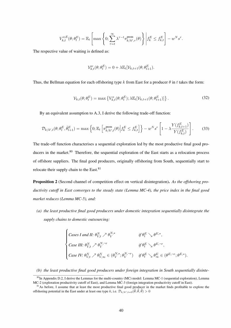
V o;Ek,t (θ; θEt ) = Et

[max

0;∞∑τ=t

λτ−tπpremk/k′,τ (θ)

∣∣∣∣∣fEk ≤ fEk,t]− wNsr.

The respective value of waiting is defined as:

Vwk,t(θ; θEt ) = 0 + λEt[Vk,t+1(θ; θEt+1).

Thus, the Bellman equation for each offshoring type k from East for a producer θ in t takes the form:

Vk,t(θ; θEt ) = maxV ok,t(θ; θ

Et );λEt[Vk,t+1(θ; θ

Et+1)]

. (32)

By an equivalent assumption to A.3, I derive the following trade-off function:

Dk/k′,t(θ; θEt , θEt+1) = max

0;Et[π

premk/k′,t(θ)

∣∣∣fEk ≤ fEk,t]− wNsr[

1− λY (fEk,t+1)

Y (fEk,t)

]. (33)

The trade-off function characterises a sequential exploration led by the most productive final good pro-

ducers in the market.80 Therefore, the sequential exploration of the East starts as a relocation process

of offshore suppliers. The final good producers, originally offshoring from South, sequentially start to

relocate their supply chain to the East.81

Proposition 2 (Second channel of competition effect on vertical disintegration). As the offshoring pro-

ductivity cutoff in East converges to the steady state (Lemma MC-4), the price index in the final good

market reduces (Lemma MC-5), and:

(a) the least productive final good producers under domestic integration sequentially disintegrate the

supply chains to domestic outsourcing:

Cases I and II: θNV,t θN,∗V if θEt θE,∗,

Case III: θNV,t θN,¬rV if θEt θE,¬r,

Case IV: θNV,t θNV,∞ ∈ (θN,∗V ; θN,¬rV ) if θEt θE∞ ∈ (θE,¬r; θE,∗).

(b) the least productive final good producers under foreign integration in South sequentially disinte-

80In Appendix D.2, I derive the Lemmas for the multi-country (MC) model: Lemma MC-1 (sequential exploration), LemmaMC-2 (exploration productivity cutoff of East), and Lemma MC-3 (foreign integration productivity cutoff in East).

81As before, I assume that at least the most productive final good producer in the market finds profitable to explore theoffshoring potential in the East under at least one type k, i.e. Dk/k′,t=0(¯θ; ¯θ, ¯θ) > 0

40

grate the supply chains to foreign outsourcing in South:

Cases I and II: θSV,t θS,∗V if θEt θE,∗,

Case III: θSV,t θS,¬rV if θEt θE,¬r,

Case IV: θSV,t θSV,∞ ∈ (θS,∗V ; θS,¬rV ) if θEt θE∞ ∈ (θE,¬r; θE,∗).

(c) starting from t, the least productive final good producers under foreign integration in East sequen-

tially disintegrate the supply chains to foreign outsourcing in East:

Cases I and II: θEV,t θE,∗V if θEt θE,∗,

Case III: θEV,t θE,¬rV if θEt θE,¬r,

Case IV: θEV,t θEV,∞ ∈ (θE,∗V ; θE,¬rV ) if θEt θE∞ ∈ (θE,¬r; θE,∗).

Proof. See Appendix D.2.7.82

Relocation and competition effect. As more final good producers explore their offshoring potential

in the East, they sequentially relocate their supply chain to this country. This allows the final good

producers to exploit the lower marginal costs offered by contracting eastern suppliers, driving the price

index further down as the sequential relocation flow to East continues.

As shown by Proposition 2, the increase in competition induces a sequential disintegration of do-

mestic and southern offshore supply chains, and from period t on, a vertical disintegration of the least

productive producers under foreign integration in East.

The increase in the competition intensity also generates the exit of the least productive producers

from the market (Lemma MC-6 (a)). An additional effect is a potential reshoring decision of the least

productive producers offshoring from the South (Lemma MC-6 (b)). However, I describe below the cases

when reshoring decisions may not be observed.

Additional considerations on equilibrium paths: Sequential institutional shocks. If the institu-

tional reform in the East takes place before the sector reaches the steady-state defined in section 3.2,

denoted here as (S), it may be possible that the reshore characterised above is not observed.83 The main82For Lemma MC-4 (convergence of offshoring productivity cutoff in East), see Appendix D.2.4. For Lemma MC-5 (price

index effect of relocation of offshore suppliers), see Appendix D.2.5. For Lemma MC-6 (convergence of market and offshoringproductivity cutoffs), see Appendix D.2.6.

83I describe here one case. For a complete analysis of the multiple equilibria with simultaneous institutional reforms, seeLarch and Navarro (2021).

41

condition is that the institutional reform in the East takes place at a period t where θSt > θS,∗O , i.e. when

the offshoring exploration cutoff in South is still above its new steady-state level. A second condition is

that the prior beliefs about eastern institutions must be optimistic enough such that the offshoring explo-

ration of the East is faster than the exploration flow to the South. Thus, the convergence of the relocation

from South to East takes place before the offshoring exploration to South finishes.

5.4 Empirical model: Competition effect in multi-country model.

I introduce an empirical model to test for both channels of the competition effect: i) the progressive

vertical disintegration that results from the increase in the competition intensity due to the increasing

offshoring activity (Proposition 1); ii) the progressive vertical disintegration that results from the reloca-

tion of the offshore suppliers towards foreign locations with lower marginal costs (Proposition 2). With

that aim, I consider a particular institutional shock in a low wage foreign country with initial low market

share in US markets: the accession of China to the WTO.

5.4.1 China access to WTO: stylized facts.

The access of China to the WTO in December 2001 has had a deep impact on the global organisation of

supply chains. Handley and Limao (2017) analyses the effect of the membership of China to the WTO

on the reduction of the tariff’s uncertainty for Chinese goods in the US. They show that, after controlling

for tariffs changes, a significant share of the export growth from China to the US is explained by the

reduction in the uncertainty about future tariffs shocks.

However, the slow increase in the imports from China relative to other foreign sourcing locations,

shown by Figure 7, may reflect effects of a residual uncertainty beyond the tariffs dimension addressed

by Handley and Limao (2017). The low market share of China in 2002 and its progressive increase in the

years following the WTO membership is in line with sectoral dynamics characterised by the theoretical

model above. Figure 7 shows that the market share of China in the US imports is growing up to 14

years after the reform, which is consistent with a sequential exploration and relocation of suppliers to

that country. In this sense, the model complements the findings in Handley and Limao (2017).

The period covered by the data on imports imposes limitations for a direct control of the Chinese

institutional shock. Nevertheless, it may still shed light on the sectoral dynamics predicted by the the-

oretical model. Figure 7a provides a first glimpse to a possible theory-consistent relation between the

penetration of China in the US market (i.e. relocation of offshore suppliers to China) and the intra-firm

import share. The negative trend in the intra-firm import share of differentiated goods may respond

42

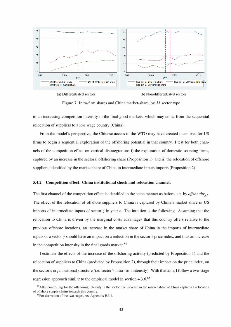
(a) Differentiated sectors (b) Non-differentiated sectors

Figure 7: Intra-firm shares and China market-share, by M sector type

to an increasing competition intensity in the final-good markets, which may come from the sequential

relocation of suppliers to a low wage country (China).

From the model’s perspective, the Chinese access to the WTO may have created incentives for US

firms to begin a sequential exploration of the offshoring potential in that country. I test for both chan-

nels of the competition effect on vertical disintegration: i) the exploration of domestic sourcing firms,

captured by an increase in the sectoral offshoring share (Proposition 1), and ii) the relocation of offshore

suppliers, identified by the market share of China in intermediate inputs imports (Proposition 2).

5.4.2 Competition effect: China institutional shock and relocation channel.

The first channel of the competition effect is identified in the same manner as before, i.e. by offshr shrj,t.

The effect of the relocation of offshore suppliers to China is captured by China’s market share in US

imports of intermediate inputs of sector j in year t. The intuition is the following. Assuming that the

relocation to China is driven by the marginal costs advantages that this country offers relative to the

previous offshore locations, an increase in the market share of China in the imports of intermediate

inputs of a sector j should have an impact on a reduction in the sector’s price index, and thus an increase

in the competition intensity in the final goods market.84

I estimate the effects of the increase of the offshoring activity (predicted by Proposition 1) and the

relocation of suppliers to China (predicted by Proposition 2), through their impact on the price index, on

the sector’s organisational structure (i.e. sector’s intra-firm intensity). With that aim, I follow a two-stage

regression approach similar to the empirical model in section 4.3.6.85

84After controlling for the offshoring intensity in the sector, the increase in the market share of China captures a relocationof offshore supply chains towards this country.

85For derivation of the two stages, see Appendix E.3.4.

43

Identification of the empirical model. In the first stage, I estimate the effect of the offshoring share

(Proposition 1) and China’s market share (Proposition 2) on the sector’s price index. I derive the follow-

ing log-linear model:

ln(Pj,t) = b0 + b1 ln(offshr shrj,t) + b2 ln(CHN mkt shrj,t) + other controls + bl + bt + uj,t (34)

In the second stage, I use the predicted value of ln(Pj,t) from the first regression and estimate its

effect on the intra-firm intensity. In other words, I use the predicted changes in the sector price index

induced by changes in the sector global offshoring activity and relocation of offshore suppliers to China.

The second stage is defined as a fractional logit model:

E[IFintl,j,t

∣∣∣x] =exp(x′

l,j,tρ)

1 + exp(x′l,j,tρ)

with x′l,j,tρ =ρ1 ln(Pj,t) + other controls + ρl + ρt. (35)

Table 5: Competition effect: Estimation in two stages.

Second stage: Main coefficient reportedAgg. countries No aggregation of countries

(1) (2) (3)IFintj,t IFintl,j,t IFintl,j,t

ln(Pj,t) -33.52∗∗∗ -23.42∗∗∗ -23.38∗∗∗

(1.981) (1.751) (1.697)FEs t t , l lt

First stage: Main coefficients(1) (2) (3)

ln(Pj,t) ln(Pj,t) ln(Pj,t)

ln(offshr shrj,t) -0.0307∗∗∗ -0.0340∗∗∗ -0.0340∗∗∗

(0.00841) (0.00961) (0.00981)

ln(CHN mrkt shrj,t) -0.00531 -0.00784∗∗ -0.00826∗∗

(0.00332) (0.00323) (0.00343)FEs t t , l ltR2 0.299 0.301 0.314Adjusted R2 0.291 0.298 0.285Second stage: Bootstrapped s.e. (1000 rep). Coefficients reported.

All stages: Cluster s.e. at sector j. Standard errors in parentheses.∗ p < 0.10, ∗∗ p < 0.05, ∗∗∗ p < 0.01

Results. The regression results are reported in Table 5.86 The results of the first stage show, as before,

that an increase in the offshoring share reduces the sector’s price index. Additionally, the results show

that an increase in China’s market share in the imports of intermediate inputs of sector j leads to a further86Full table is reported in Table 15 in Appendix E.3.4.

44

reduction in the price index. Therefore, as more final good producer relocate their offshore suppliers to

China, the competition in the final good market intensifies. The empirical evidence is consistent with the

theoretical predictions on the two channels that intensify the competition in the final goods market.

The results of the second stage show supportive evidence for the vertical disintegration consequences

of the competition effect characterised by the theoretical model above. It shows that the sector’s price

index reductions predicted by both channels in the first stage regression result in lower intra-firm intensity

in the sector. To sum up, the regression results are consistent with the predictions of the model and

provide supportive evidence for Propositions 1 and 2.

6 The role of FTAs and MAs on exploration decisions

I develop a simple theoretical extension of the model to characterise the role that free trade agreements

(FTAs) and multilateral agreements (MAs) may play as exploration triggers of new sourcing locations.

I highlight specific features of FTAs and MAs that may lead to novel effects on exploration decisions

when firms face institutional uncertainty.

6.1 Role of FTAs.

I consider the role of the FTAs from two dimensions: the preferential tariffs and the institutional ar-

rangements. The first refers to the reduction in bilateral tariffs among the members of the FTAs. The

second comprehends the institutional commitments and regulations agreed by the members that consti-

tute the institutional framework of the FTAs (Maggi, 1999; Dur et al., 2014; Limao, 2016). It includes

areas such as: intellectual property and property rights protection, foreign investment, dispute resolution

mechanisms, environmental regulation, labour market regulations and mobility.87

I begin with the role of preferential tariffs on the exploration decisions of new locations. I follow

with the role of the institutional dimension of the FTAs as information shocks on the prior beliefs that

may lead to exploration of new locations and thus sequential offshoring and relocation processes.

6.1.1 Role of FTAs: tariff dimension.

I define the marginal cost for a northern producer of an intermediate input sourced from l as clt = τ lm,twl,

where τ lm,t captures the associated trade costs relative to the location l = N,E, S. I define it as τ lm,t = 1

87For examples of this type of regulations involved in FTAs see NAFTA: www.naftanow.org, EU: europa.eu, Pacific Alliance:alianzapacifico.net/en, MERCOSUR: www.mercosur.int, China-Australia (ChAFTA): www.dfat.gov.au/trade/agreements/in-force/chafta/Pages/australia-china-fta.

45

when the tariffs are zero with respect to the country l. Therefore, τNm,t = 1 ∀ t.

Two-country model: North-South FTA. The initial conditions are defined by free trade in the final

goods and positive tariffs in the intermediate inputs, i.e. τSm,t > 1 for any t < 0. In t = 0, a FTA between

North and South is signed and all tariffs are removed, i.e. τSm,t = 1 ∀ t ≥ 0. I consider that the FTA

is limited to a tariff reduction and has no implications in terms of institutional reforms. Therefore, the

priors about the southern institutions are not directly affected by the agreement.

If tariffs in intermediate inputs previous to the FTA are large enough, such that cSt > cNt , no final good

producer finds it profitable to offshore from the South independently of the uncertainty about southern

institutions. In other words, θSO > ¯θ and θSV > ¯θ. Instead, when initial tariffs are small enough such

that cSt < cNt , it may be possible that under perfect information, some final good producers would have

found it profitable to offshore from the South. However, when the prior beliefs about southern institutions

are pessimistic, it may discourage all the northern final good producers from exploring their offshoring

potential in South. This situation takes place when the following condition holds for any t < 0:88

Dk,t(¯θ; ¯θ, ¯θ, τSm,t) < 0 for all k = O, VH , VM .

If the tariff reduction introduced by the FTA is large enough, it may induce the offshoring exploration

at the given prior beliefs for at least the most productive producers in the market:

Dk,t=0(¯θ; ¯θ, ¯θ, τSm,t) ≥ 0 for at least one k = O, VH , VM .

Once the exploration begins, the information spillovers drive the sector to the perfect information steady-

state, as characterised in Section 3.2.

Multicountry-model: North-East FTA. I extend the previous case to a multi-country setup. As be-

fore, initially, offshoring is only profitable in the South. There is free trade in the final goods but the

northern country sets positive tariffs on intermediate inputs, i.e. τSm,t = τEm,t > 1. To avoid a taxonomy

of cases, I assume that at the current tariffs, the marginal costs of the intermediate inputs for the final

good producers from each location are: cEt < cSt < cNt . Under perfect information, some final good

producers would find it profitable to offshore in the East.

When the prior beliefs about eastern institutions are too pessimistic, no final good producer finds it

attractive to explore the offshoring potential from the East at the given tariffs. Thus, for any t < 0:

Dk/k′,t(¯θ; ¯θE , ¯θE , τEm,t, τSm,t) < 0 for all k = O, VH , VM .

88 ¯θ indicates the most productive final good producer in the differentiated sector. A necessary condition is that the supportof the distribution G(θ) is bounded to the right, i.e. ¯θ <∞.

46

In t = 0 the FTA between North and East takes place, and the tariffs on intermediate inputs are

removed for eastern suppliers, i.e. τEm,t = 1. As before, the FTA is limited to an agreement on tariffs.

Thus, the prior beliefs about eastern institutions are not directly affected by the FTA.

If the change in tariffs induces a large enough reduction in the marginal cost cEt relative to cSt , the

most productive final good producers currently offshoring in South may find it profitable to explore East

for a potential relocation of suppliers. The FTA triggers the sequential exploration of East if:

Dk/k′,t=0(¯θ; ¯θE , ¯θE , τEm,t, τSm,t) ≥ 0 for at least one k = O, VH , VM .

The sequential exploration drives the sector to the perfect information steady-state, as in section 5.

Summing up, preferential tariffs may have a stronger effect compared to an approach that neglects

the presence of institutional uncertainty. When institutional uncertainty is present, small reductions in

intermediate input tariffs may create enough incentives for the most productive final good producers in

the market to explore the offshoring potential in those locations, and thus trigger the sequential offshoring

equilibrium paths characterised above.

6.1.2 Role of FTAs: institutional dimension.

I analyse the role of the institutional dimension for two types of FTAs: i) the signature of a FTA with

North, ii) the signature of a FTA among third countries where the North is not a member of the agreement.

Additionally, I study the role of MAs, in particular, the access to a WTO membership. I show that these

shocks may impact the prior beliefs that northern producers possess about foreign locations and thus

create incentives to explore the offshoring potential in those countries.

FTAs with North. The implementation of a FTA usually goes beyond reductions in tariffs and incor-

porates institutional aspects (Dur et al., 2014). Therefore, the signature of a FTA reveals a commitment

of the governments to provide an institutional environment that meets the set of specified rules.

When a FTA between the North (US in the empirical model) and a foreign location is signed, the

institutional framework is observable by the northern producers. Thus, if the institutional priors about

the partner country were relatively pessimistic, the FTA may positively affect the beliefs.

FTAs among third countries. The FTAs signed among third countries, where the North (US) is not

involved, may also reveal information to the northern producers about the institutional conditions in the

countries involved in the agreement. When a FTA is under negotiation, countries with good institutional

47

fundamentals may not want to expose themselves to trade with partners under poor institutional condi-

tions, while countries with bad institutional fundamentals may want to avoid strict rules that they cannot

enforce. Thus, the institutional framework of the FTA emerges as the result of a bargaining on a set of

rules that regulate the relationships among the members.

The northern final good producers may associate the FTA among third countries to the revelation of a

common institutional ground among the members. Therefore, the countries with relatively worse priors

may benefit from those with a better institutional reputation. The priors related to the first countries, i.e.

those with worse priors, may experience a positive shock, and thus the FTA may promote the offshoring

exploration in those locations.

MAs: WTO membership. The access of a country to a WTO membership reveals information regard-

ing regulations that members of the organisation must follow. It may affect the prior beliefs that northern

producers possess about the institutional conditions in that location.

Modelling of the prior’s shock. I assume that initially, the prior beliefs of northern producers in sector

j about country l institutions before any shock takes place are given by:

f lk,j ∼ Yj(f lk,j) with f lk,j ∈[f lk,j , f

lk,j

]and k = O, VH , VM .

As already mentioned, FTAs and MAs are institutional shocks that reveal information about rules

to which the government of country l has committed to enforce. In other words, it reveals the minimal

institutional conditions in the country l. In the model, it is captured by a reduction in the upper bound de-

fined by the initial prior, only when prior to the shock the institutional beliefs were relatively pessimistic.

Formally, the prior institutional uncertainty at any period t is given by:

f lk,j ∼ Yj(f lk,j) with f lk,j ∈[f lk,j , f

lk,j − Ilk,j,t

],

where f lk,j refers to the initial upper bound of the prior distribution, and Ilk,j,t refers to the institutional

information revealed by FTAs and MAs shocks experienced by a non-explored location l up to period t.

Ilk,j,t is defined as:

Ilk,j,t ≡ max1[dUSl,t = 1

]FTAUS

k,l;1[dWTOl,t = 1

]WTOk,l;1

[dFTA:3rdl,t = 1

]FTA3rd

k,l

where dUS

l,t is a dummy that refers to the existence of a FTA between the North (US) and country l in

48

period t, dWTOl,t is a dummy that indicates the WTO membership of country l in period t, and dFTA:3rd

l,t is a

dummy that indicates that country l has a FTA with third countries in period t.

The variable FTAUSk,l refers to the institutional information revealed by a FTA between the North and

country l, i.e. by the institutional commitment revealed by the agreement. The variable FTA3rdk,l represents

the institutional information revealed by a FTA that country l signs with third countries. Finally, WTOk,l

denotes the upper bound defined by the WTO institutional framework. All these variables are defined in

[0,∞] and they are increasing in the information revealed by the respective FTA or MA.

6.2 Empirical model: The role FTAs on exploration decisions.

6.2.1 Data.

I use data on US imports classified at HS codes (6 digits) from UN Comtrade. The main advantage of

this dataset is the longer sample period (1996-2016), which allows me to cover a higher number of WTO

accessions and the formation of new FTAs and new memberships of countries to pre-existing FTAs. A

second advantage comes from the higher disaggregation of the data, which provides a higher variation

of foreign countries’ first-time exploration decisions for each product code.

The Rule of Law index comes from the World Governance Indicators of the World Bank database,

the data on GDP per capita and GDP from the World Development Indicator of the World Bank. I use

the data on distance and common official language from CEPII. Finally, the data on FTA comes from an

updated version of “Mario Larch’s Regional Trade Agreements Database from Egger and Larch (2008)”.

6.2.2 Identification: definition of main variables.

I identify the tariff dimension of the FTAs by controlling for bilateral tariffs. Regarding the institutional

dimension of the FTAs, I identify the three types of shocks characterised in section 6.1.2: i) the signature

of a FTA with the US, ii) the access to WTO membership, iii) the signature of a FTA with third countries.

The prior beliefs about the institutional conditions in country l in year t are captured by the respective

Rule of Law index. This index is built based on surveys. Therefore, instead of being a direct measure of

the institutional fundamentals, it is closer to capturing the perceptions about the institutional conditions

in each country. In the latter sense, it is a suitable proxy for the prior beliefs about the institutional

conditions in each location.89 I define the Rule of Law index by the exponential function of the original89”Rule of Law captures perceptions of the extent to which agents have confidence in and abide by the rules of society, and

in particular the quality of contract enforcement, property rights, the police, and the courts, as well as the likelihood of crimeand violence”. World Bank http://info.worldbank.org/governance/wgi/Home/Documents. For methodological information seeKaufmann et al. (2011). See Larch and Navarro (2021) for further discussions.

49

value reported in WGI, such that it is defined in (0,∞).

I identify the first type of shock as FTAUSl,t , which captures the institutional differential between the

US and the prior beliefs of country l at the moment t′ when it signs a FTA with US. When prior beliefs

about institutions in country l are better than in US, FTAUSl,t takes value zero, i.e. the agreement provides

no additional information about the institutional conditions in l. Thus, FTAUSl,t is given by:90

FTAUSl,t =

max

RLUSt′ − RLl,t′ , 0

if l access the FTA in t′ ≤ t

0 otherwise

The effect of the access to WTO membership is captured by the variable WTOl,t. It takes the value

one from the period when country l becomes a member of WTO, and zero otherwise.91

I identify the FTAs among third countries by the variable FTA3rdl,t defined in [0,∞). When country

l becomes a member of a FTA with third countries, the variable measures the additional information

revealed by the agreement about institutions in the country l. To capture this, the variable takes the

maximum value between the mean institutional quality of the members of the agreement at the year that

the country l becomes part of it, and the Rule of Law index of country l in that same year. In other words,

it captures the additional information revealed by the agreement over the direct perception of institutional

conditions. Thus, FTA3rdl,t is given by:92

FTA3rdl,t =

max

RLFTA3rd

l,t′ ,RLl,t′

if l access the FTA in t′ ≤ t

0 otherwise

where RLFTA3rdl,t′ denotes the mean value of the Rule of Law indices of all the countries that are part of

the agreement in the accession year t′.

If the country signs multiple FTAs during the sample period, the variable takes the value of new FTAs

only when new information is revealed. For instance, consider the situation where country l signs a FTA

”A” in year t′ and a FTA ”B” in year t′′ with t′ < t′′. The variable FTA3rdl,t is:

FTA3rdl,t =

max

RLFTA3rd:”A”l,t′ , RLl,t′

if t′ ≤ t

max

RLFTA3rd:”A”l,t′ ,RLFTA3rd:”B”l,t′′ , RLl,t′

if t′′ ≤ t

0 otherwise

90It considers only those FTAs signed during the sample period. Previous FTAs are captured by country fixed effects.91It considers only new memberships during the sample period. Previous memberships are captured by country fixed effects.92It considers only those FTAs signed during the sample period. Previous FTAs are captured by country fixed effects.

50

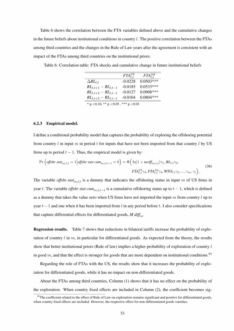
Table 6 shows the correlation between the FTA variables defined above and the cumulative changes

in the future beliefs about institutional conditions in country l. The positive correlation between the FTAs

among third countries and the changes in the Rule of Law years after the agreement is consistent with an

impact of the FTAs among third countries on the institutional priors.

Table 6: Correlation table: FTA shocks and cumulative change in future institutional beliefs

FTAUSl,t FTA3rd

l,t

∆RLl,t -0.0228 0.0503***RLl,t+1 − RLl,t−1 -0.0185 0.0533***RLl,t+2 − RLl,t−1 -0.0127 0.0908***RLl,t+3 − RLl,t−1 -0.0104 0.0804**** p <0.10, ** p <0.05 , *** p <0.01

6.2.3 Empirical model.

I define a conditional probability model that captures the probability of exploring the offshoring potential

from country l in input m in period t for inputs that have not been imported from that country l by US

firms up to period t− 1. Thus, the empirical model is given by:

Pr(

offshr statm,l,t = 1∣∣∣offshr stat cumm,l,t−1 = 0

)= Φ

(ln(1 + tariffm,l,t)γ1,RLl,tγ2,

FTAUSl,tγ3,FTA3rd

l,t γ4,WTOl,tγ5, ..., γm, γt

),

(36)

The variable offshr statm,l,t is a dummy that indicates the offshoring status in input m of US firms in

year t. The variable offshr stat cumm,l,t−1 is a cumulative offshoring status up to t− 1, which is defined

as a dummy that takes the value zero when US firms have not imported the input m from country l up to

year t− 1 and one when it has been imported from l in any period before t. I also consider specifications

that capture differential effects for differentiated goods, M diffm.

Regression results. Table 7 shows that reductions in bilateral tariffs increase the probability of explo-

ration of country l in m, in particular for differentiated goods. As expected from the theory, the results

show that better institutional priors (Rule of law) implies a higher probability of exploration of country l

in good m, and that the effect is stronger for goods that are more dependent on institutional conditions.93

Regarding the role of FTAs with the US, the results show that it increases the probability of explo-

ration for differentiated goods, while it has no impact on non-differentiated goods.

About the FTAs among third countries, Column (1) shows that it has no effect on the probability of

the exploration. When country fixed effects are included in Column (2), the coefficient becomes sig-93The coefficient related to the effect of Rule of Law on exploration remains significant and positive for differentiated goods,

when country fixed effects are included. However, the respective effect for non-differentiated goods vanishes.

51

Table 7: Conditional probability model: Institutional shocks and exploration decisions

Exp. (1) (2) (3) (4)sign offshr statm,l,t offshr statm,l,t offshr statm,l,t offshr statm,l,t

ln(1 + tariffm,l,t) - -0.483∗∗∗ -0.508∗∗∗ -0.0173 0.0106(0.0660) (0.0671) (0.117) (0.120)

RLl,t + 0.0661∗∗∗ 0.0104 0.0315∗∗∗ -0.0142(0.00319) (0.00787) (0.00698) (0.0103)

FTAUSl,t + 0.0289∗∗∗ -0.000269 0.00812 -0.0158∗

(0.00303) (0.00374) (0.00832) (0.00856)

WTOl,t + 0.230∗∗∗ 0.160∗∗∗ 0.142∗∗∗ 0.117∗∗∗

(0.00782) (0.0144) (0.0230) (0.0266)

FTA3rdl,t 0.00188 -0.0286∗∗∗ -0.0245∗∗∗ -0.0587∗∗∗

(0.00264) (0.00360) (0.00631) (0.00673)

ln(1 + tariffm,l,t)×M diffm - -0.891∗∗∗ -1.018∗∗∗

(0.187) (0.194)

RLl,t ×M diffm + 0.0480∗∗∗ 0.0335∗∗∗

(0.00787) (0.00807)

FTAUSl,t ×M diffm + 0.0238∗∗ 0.0178∗

(0.00961) (0.00965)

WTOl,t ×M diffm + 0.103∗∗∗ 0.0461∗

(0.0258) (0.0267)

FTA3rdl,t ×M diffm + 0.0352∗∗∗ 0.0394∗∗∗

(0.00728) (0.00730)FEs t , HS4dig t , HS4dig , l t , HS4dig t , HS4dig , lOther controls in columns (1) and (3): ln(distl), ln( ¯GDPpcl), ln( ¯GDPl), common official langl.

Robust standard errors in parentheses. ∗ p < 0.10, ∗∗ p < 0.05, ∗∗∗ p < 0.01

nificant and negative. This effect is consistent with a trade diversion effect, while it does not provide

evidence in favour of the mechanism predicted by the model. Columns (3) and (4), instead, show that it

positively affects the exploration decisions for differentiated goods relative to non-differentiated goods.

The negative effect for non-differentiated goods is still in line with an expected trade diversion effect. In-

stead, the positive and significant coefficient related to the interaction term provides supportive evidence

for their role as institutional information shocks on priors. The information revealed by FTA3rd positively

affects the exploration decisions in goods that rely more on the institutional environment.

Finally, the empirical evidence shows that access to WTO membership promotes offshoring explo-

ration.94 This is in line with the model’s predictions considering that the accession to the WTO reveals94The results are consistent with the theoretical predictions and the literature that have already analysed entry decisions after

WTO accessions (Handley and Limao, 2017; Handley et al., 2020).

52

a commitment of country l to a general set of rules in a multilateral agreement. As expected from the

theory, the effect is stronger for differentiated goods.

7 Conclusions

I develop a dynamic model on global sourcing where the final good producers face uncertainty about

institutional conditions in foreign countries when deciding the organisation of their supply chain. The

model centers the attention on the dynamic allocation of property rights. I introduce first a model in a

two-country setup (North-South), where northern final good producers face uncertainty about the south-

ern institutional conditions. Later, I extend it to multiple countries.

I characterise the underlying learning mechanism and the trade-off decisions that the final good pro-

ducers face when they decide whether to explore their offshoring potential in a foreign location or wait,

and the resulting sectoral equilibrium organisational dynamics. The main result is that the sequential

increase in the offshoring activity progressively reduces the price index in the final good markets, which

translates into a higher intensity in the competition in the final goods market. This leads to a progres-

sive vertical disintegration of the supply chains (Proposition 1: first channel of the competition effect on

vertical disintegration).

In the multi-country extension, I show that when final good producers under offshoring decide to

explore new locations with lower marginal costs, they may trigger a sequential relocation of offshore

suppliers towards those countries. The lower marginal costs offered by the new sourcing locations push

the sector’s price index further down, reinforcing the vertical disintegration trend (Proposition 2: second

channel of the competition effect on vertical disintegration).

Using US manufacturing sector-level data for 2002-2016, I find evidence on sectoral dynamics that

supports both channels of the competition effect. Regarding the first channel, I find that as the offshoring

activity in a sector increases, the price index reduces, which leads to a progressive reduction in the

intra-firm intensity of the sector. Regarding the second channel, I focus on the analysis of one specific

institutional shock: the access of China to the WTO. Considering the low wage of China and its initial low

market share in US markets, I identify the effect of a relocation towards a country with lower marginal

costs. The empirical results show that as the relocation of offshore suppliers to China advances, the price

index reduces, pushing for a reduction in the intra-firm intensity sector.

Finally, I analyse the role of FTAs as triggers of the exploration decisions of new locations. The

role of FTAs is analysed from two dimensions: preferential tariffs and institutional arrangements.95 The95Regarding the tariff dimension, the model shows that if the prior beliefs about institutions in the partner country previous to

53

main focus is on the institutional dimension of FTAs, and their role as information shocks on institutional

priors. The signature of a FTA reveals a commitment of the signing governments to provide an institu-

tional environment that meets the set of rules specified in the agreement. If those rules are observable by

northern firms, a new FTA impacts on the prior beliefs about the partner-country and thus incentivise the

offshoring exploration of the country.

From this perspective, the model also shows that FTAs among third countries may affect countries’

priors beliefs and thus potentially create incentives to explore those locations by northern firms. In

particular, when the final good producers associate the FTA to some common institutional ground among

the members of the FTA, the countries with relatively worse priors may benefit from those with a better

institutional reputation.

As an additional dimension, I also analyse the role of multilateral agreements (MAs) as information

shocks on prior beliefs. In particular, I focus on the access to WTO memberships. This membership re-

veals the members’ commitment to a general institutional framework, which may impact on the previous

pessimistic priors about the new members and thus promote the offshoring exploration of those countries

by northern firms.

Using import data at HS 6 digits for the period 1996-2016 from UN Comtrade, I test for the role

of these types of institutional shocks as incentives to explore those locations where the US final good

producers have not explored their offshoring potential. I identify three types of shocks: the signature of

a FTA where the US is involved; the signature of a FTA where the US is not involved; and the accession

to the WTO membership. The empirical results provide support for the predictions of the model.

the FTA are pessimistic, no final good producer find it attractive to explore the offshoring in that country. When the reductionsin tariffs for intermediate inputs are sufficiently large, it may create enough incentives to trigger a sequential exploration ofthat country by at least the most productive final good producers. Thus, small changes in the tariffs may induce a sectoralreorganisation that extends beyond the expected changes that arise from an approach that ignores the presence of institutionaluncertainty.

54

References

Aeberhardt, R., Buono, I. and Fadinger, H. (2014), ‘Learning, incomplete contracts and export dynamics:

theory and evidence from french firms’, European Economic Review 68, 219–249.

Albornoz, F., Pardo, H. F. C., Corcos, G. and Ornelas, E. (2012), ‘Sequential exporting’, Journal of

International Economics 88(1), 17–31.

Alfaro, L. and Charlton, A. (2009), ‘Intra-industry foreign direct investment’, American Economic Re-

view 99(5), 2096–2119.

Antras, P. (2003), ‘Firms, contracts, and trade structure’, The Quarterly Journal of Economics

118(4), 1375–1418.

Antras, P. (2005), ‘Incomplete contracts and the product cycle’, American Economic Review 95(4), 1054–

1073.

Antras, P. (2015), Global production: Firms, contracts, and trade structure, Princeton University Press.

Antras, P. and Chor, D. (2013), ‘Organizing the global value chain’, Econometrica 81(6), 2127–2204.

Antras, P. and Chor, D. (2021), Global value chains, Working Paper 28549, National Bureau of Economic

Research.

Antras, P. and Helpman, E. (2004), ‘Global sourcing’, Journal of Political Economy 112(3), 552–580.

Antras, P. and Helpman, E. (2008), Contractual Frictions and Global Sourcing, Harvard University

Press, Cambridge, MA, pp. 9–54.

Antras, P. and Staiger, R. W. (2012), ‘Offshoring and the role of trade agreements’, American Economic

Review 102(7), 3140–83.

Araujo, L., Mion, G. and Ornelas, E. (2016), ‘Institutions and export dynamics’, Journal of International

Economics 98, 2–20.

Blanchard, E. (2019), ‘Trade wars in the global value chain era’, Trade War: The Clash of Economic

Systems Endangering Global Prosperity pp. 57–63.

Bown, C. P., Conconi, P., Erbahar, A. and Trimarchi, L. (2021), ‘Trade protection along supply chains’.

Broda, C. and Weinstein, D. E. (2006), ‘Globalization and the gains from variety’, The Quarterly journal

of economics 121(2), 541–585.

55

Carballo, J. (2016), Global sourcing under uncertainty, Technical report, University of Colorado, mimeo.

Coase, R. H. (1937), ‘The nature of the firm’, Economica 4(16), 386–405.

Dosi, G., Nelson, R. R., Winter, S. G. et al. (2000), The nature and dynamics of organizational capabili-

ties, Oxford university press.

Dur, A., Baccini, L. and Elsig, M. (2014), ‘The design of international trade agreements: Introducing a

new dataset’, The Review of International Organizations 9(3), 353–375.

Egger, P. and Larch, M. (2008), ‘Interdependent preferential trade agreement memberships: An empirical

analysis’, Journal of International Economics 76(2), 384–399.

Feenstra, R. C. (1998), ‘Integration of trade and disintegration of production in the global economy’,

Journal of Economic Perspectives 12(4), 31–50.

Felbermayr, G., Larch, M., Yalcin, E. and Yotov, Y. (2020), ‘On the heterogeneous trade and welfare

effects of gatt/wto membership’.

Gereffi, G., Humphrey, J. and Sturgeon, T. (2005), ‘The governance of global value chains’, Review of

International Political Economy 12(1), 78–104.

Gereffi, G., Lim, H.-C. and Lee, J. (2021), ‘Trade policies, firm strategies, and adaptive reconfigurations

of global value chains’, Journal of International Business Policy pp. 1–17.

Grossman, G. M. and Helpman, E. (2002), ‘Integration versus outsourcing in industry equilibrium’, The

Quarterly Journal of Economics 117(1), 85–120.

Grossman, G. M. and Helpman, E. (2004), ‘Managerial incentives and the international organization of

production’, Journal of International Economics 63(2), 237–262.

Grossman, G. M. and Helpman, E. (2005), ‘Outsourcing in a global economy’, The Review of Economic

Studies 72(1), 135–159.

Grossman, G. M. and Helpman, E. (2020), When tariffs disturb global supply chains, Technical report,

National Bureau of Economic Research.

Grossman, S. J. and Hart, O. D. (1986), ‘The costs and benefits of ownership: A theory of vertical and

lateral integration’, Journal of Political Economy 94(4), 691–719.

56

Handley, K. and Limao, N. (2017), ‘Policy uncertainty, trade, and welfare: Theory and evidence for

china and the united states’, American Economic Review 107(9), 2731–83.

Handley, K., Limao, N., Ludema, R. D. and Yu, Z. (2020), Firm input choice under trade policy uncer-

tainty, Technical report, National Bureau of Economic Research.

Hart, O. and Moore, J. (1990), ‘Property rights and the nature of the firm’, Journal of Political Economy

98(6), 1119–1158.

Head, K. and Mayer, T. (2019), ‘Brands in motion: How frictions shape multinational production’,

American Economic Review 109(9), 3073–3124.

Helpman, E. (2006), ‘Trade, fdi, and the organization of firms’, Journal of Economic Literature

44(3), 589–630.

Johnson, R. C. and Noguera, G. (2012), ‘Accounting for intermediates: Production sharing and trade in

value added’, Journal of International Economics 86(2), 224–236.

Kaufmann, D., Kraay, A. and Mastruzzi, M. (2011), ‘The worldwide governance indicators: Methodol-

ogy and analytical issues1’, Hague journal on the rule of law 3(2), 220–246.

Kohler, W. and Kukharskyy, B. (2019), ‘Offshoring under uncertainty’, European Economic Review

118, 158–180.

Larch, M. and Navarro, L. (2021), ‘Uncertainty in global sourcing: Learning, sequential offshoring, and

selection patterns’, mimeo .

Levchenko, A. A. (2007), ‘Institutional quality and international trade’, The Review of Economic Studies

74(3), 791–819.

Limao, N. (2016), Preferential trade agreements, in ‘Handbook of commercial policy’, Vol. 1, Elsevier,

pp. 279–367.

Maggi, G. (1999), ‘The role of multilateral institutions in international trade cooperation’, American

Economic Review 89(1), 190–214.

Melitz, M. J. (2003), ‘The impact of trade on intra-industry reallocations and aggregate industry produc-

tivity’, Econometrica 71(6), 1695–1725.

57

Nelson, R. R. (1995), ‘Recent evolutionary theorizing about economic change’, Journal of economic

literature 33(1), 48–90.

Nelson, R. R. and Winter, S. G. (1982), An Evolutionary Theory of Economic Change, Harvard Univer-

sity Press.

Nelson, R. R. and Winter, S. G. (2002), ‘Evolutionary theorizing in economics’, Journal of economic

perspectives 16(2), 23–46.

Nguyen, D. X. (2012), ‘Demand uncertainty: Exporting delays and exporting failures’, Journal of Inter-

national Economics 86(2), 336–344.

Nunn, N. (2007), ‘Relationship-specificity, incomplete contracts, and the pattern of trade’, The Quarterly

Journal of Economics 122(2), 569–600.

Nunn, N. and Trefler, D. (2013), ‘Incomplete contracts and the boundaries of the multinational firm’,

Journal of Economic Behavior & Organization 94, 330–344.

Ornelas, E. and Turner, J. L. (2008), ‘Trade liberalization, outsourcing, and the hold-up problem’, Jour-

nal of International Economics 74(1), 225–241.

Ornelas, E. and Turner, J. L. (2012), ‘Protection and international sourcing’, The Economic Journal

122(559), 26–63.

Ornelas, E., Turner, J. L. and Bickwit, G. (2020), ‘Preferential trade agreements and global sourcing’,

mimeo .

Ramondo, N., Rappoport, V. and Ruhl, K. J. (2013), ‘The proximity-concentration tradeoff under uncer-

tainty’, Review of Economic Studies 80(4), 1582–1621.

Rauch, J. E. (1999), ‘Networks versus markets in international trade’, Journal of International Eco-

nomics 48(1), 7–35.

Rob, R. (1991), ‘Learning and capacity expansion under demand uncertainty’, The Review of Economic

Studies 58(4), 655–675.

Rob, R. and Vettas, N. (2003), ‘Foreign direct investment and exports with growing demand’, The Review

of Economic Studies 70(3), 629–648.

58

Segura-Cayuela, R. and Vilarrubia, J. M. (2008), Uncertainty and entry into export markets, Technical

report, Banco de Espana working paper.

Teece, D. J. (2009), Dynamic capabilities and strategic management: Organizing for innovation and

growth, Oxford University Press.

Van Assche, A. and Gangnes, B. (2019), ‘Global value chains and the fragmentation of trade policy

coalitions’, Transnational Corporations Journal 26(1).

Williamson, O. E. (1971), ‘The vertical integration of production: market failure considerations’, The

American Economic Review 61(2), 112–123.

Williamson, O. E. (1979), ‘Transaction-cost economics: the governance of contractual relations’, The

Journal of Law and Economics 22(2), 233–261.

Williamson, O. E. (1985), The Economic Institutions of Capitalism: Firms, markets, relational Contract-

ing, Free Press.

Yeaple, S. R. (2006), ‘Offshoring, foreign direct investment, and the structure of us trade’, Journal of the

European Economic Association 4(2-3), 602–611.

59

A Perfect information model

Under perfect information, I eliminate the time index to simplify the notation.

A.1 Consumer’s problem

The budget constraint is given by:

p0q0 +

J∑j=1

∫i∈Ij

pj(i)qj(i)di ≤ E.

Given the utility function defined by equation (1), γjE refers to the expenditure in varieties of the

differentiated sector j. Thus, the demand function for a variety i in differentiated sector j is:

qj(i) =

[γjEQ

−αjj pj(i)

−1

]σj.

The demand for homogeneous good is given by: q0 = γ0Ep0

.

A.2 Appendix to organisational choice: backward induction solution.

A.2.1 Nash Bargaining

Plugging the equation (3) into the expression for revenues: r(i) = γEQ−αq(i)α−1q(i). Replacing with

the production level of variety with the production technology (5), I get:

r(i) = γEQ−αθα

[(xh(i)

η

)η (xm(i)

1− η

)1−η]α

.

The Nash bargaining equilibrium comes from the solution to the following problem:

arg maxz

Ω = [zr(i)− ωh]β [(1− z)r(i)− ωm]1−β .

From solving the FOC, I get:

z = β +(1− β)ωh − βωm

r(i).

Outsourcing (O). Both parties remain as independent specialised firms. Therefore, they keep control

over their respective assets and the inputs produced from their use. If they do not reach an agreement,

they receive their respective outside options, ωh = ωm = 0. Instead, if they agree, the final good variety

is produced and the revenues are divided according to the Nash bargaining and the equilibrium shares are

defined by z = β. Thus, the final good producer H receives the share βlO = β and the supplier receives

1− βlO = 1− β, where l denotes the location of the supplier M .

60

Backward integration (VH ). The final good producer H owns both types of assets. If she and the

manager of M fail to reach an agreement, they both receive their respective outside options. The final

good producer can fire the manager and seize the manufacturing facilities. Thus, H can use the assets at

the supplier’s location to produce the intermediate inputs without the latter’s cooperation.

Under the non-cooperative outcome, H faces an efficiency loss in the production of the intermediate

inputs, which is represented by 1 − δlVH with δlVH ∈ (0, 1). When H fires the manager of M , she may

involuntarily induce a disruption on routines and tacit knowledge at the supplier’s facilities (Nelson and

Winter, 1982; Dosi et al., 2000).96 As a consequence, H faces an efficiency loss in the manufacturing

process of the intermediate input for a given level of investment m(i) in relationship-specific assets.

Moreover, given the firm-specific nature of the routines and tacit knowledge, the outside option of the

manager of M is still zero. The outside option of the final good producer is ωh = (δlVH )α(1−η)r(i),

where r(i) denote the revenues if the parties reach an agreement (cooperate).97

If the parties cooperate, the Nash bargaining equilibrium leads to revenue shares given by:

Final good producer: βlVH = (δlVH )α(1−η) + β[1− (δlVH )α(1−η)],

Supplier: (1− βlVH ) = (1− β)[1− (δlVH )α(1−η)],

where βlVH is the revenue share of H under backward integration with a supplier M located in country

l.98 Figure 8 shows βlVH as a function of η and δlVH .

Forward integration (VM ). The manufacturer M owns both types of assets. Thus, M can fire the

manager of H after the investment in relationship-specific assets and seized the northern facilities. M

can thus take control of the production of the H-services and the final good variety.

Under the non-cooperative outcome, due to the destruction of tacit knowledge and disruption of

routines at the final good production facilities, M faces an efficiency loss in the production of the final

good producer services xh represented by 1− δlVM with δlVM ∈ (0, 1). Thus, the revenue realised by M

is (δlVM )αηr(i), which defines his ωm under forward integration. Given the firm-specific nature of the

routines and tacit knowledge, the manager of H has an outside option equal to zero.96They identify non-codifiable knowledge and routines as key determinants of a firm’s (supplier’s) productivity.97The efficiency loss can easily include a general loss in the production of both inputs as in Antras and Helpman (2004),

together with a specific additional loss in the seized input. The first loss may be related to the higher complexity involvedin the management of both facilities by H , while the second loss relates to the destruction of tacit knowledge and routinesin the supplier’s facilities. In such a case, the production of the variety would be given by (δl + (δlm,VH )1−η)q(i), where(1 − δl) refers to the general loss and (1 − δm,VH ) refers to the input m specific dimension. Therefore, in terms of revenues:(δl + (δlm,VH )1−η)αr(i).

98By the upfront payment that the final good producer establishes in the contract, no rents are left to the supplier and M ’sparticipation constraint binds.

61

Figure 8: H’s revenues share - backward integration, βlVH (η, δlVH ). [β = 0.5, α = 0.4]

If the parties agree, the Nash bargaining equilibrium results in revenue shares:

Final good producer: βlVM = β[1− (δlVM )αη],

Supplier: (1− βlVM ) = (δlVM )αηr(i) + (1− β)[1− (δlVM )αη],

where βlVM denotes the revenue share of H under forward integration with a supplier located in l.99

Figure 9 shows βlVM as a function of η and δlVM .

Figure 9: H’s revenues share - forward integration, βlVM (η, δlVM ). [β = 0.5, α = 0.4]

99By the upfront payment that the final good producer establishes in the contract, no rents are left to the supplier and M ’sparticipation constraint binds.

62

A.2.2 Investment decisions and input provision.

Both parties internalise the respective revenue shares βlk in their investment decisions. The investments

in the relationship-specific assets h(i),m(i) require the use of labour according to the constant return

technologies: hlk(i) = `lh,k(i) and mlk(i) = `lm,k, where l denotes the location of M and k = O, VH , VM

indicates the type of ownership structure.100

The ex-post production levels of the respective inputs for the variety i are a function of the ex-ante

investment decisions in the specific assets, and they are given by: xlh,k(i) = hlk(i) and xlm,k(i) = mlk(i).

The parties decide their respective investment by solving their respective maximisation programs, which

are given by:

Final-good producer’s program: maxxlh,k(i)

πlH,k = βlkrlk(x

lh,k(i))− wNxlh,k(i)− wNf lk,

Supplier’s program: maxxlm,k(i)

πlM,k = (1− βlk)rlk(xlm,k(i))− wlxlm,k(i).

From the FOCs, I derive the optimal investment levels for each party, the respective revenues, and

the total output of variety i. The optimal investment levels and input production of each party are:

hl,∗k (θ) = xl,∗h,k(θ) =αβlkη

wNrl,∗k (θ),

ml,∗k (θ) = xl,∗m,k(θ) =

α(1− βlk)(1− η)

wlrl,∗k (θ),

with k = O, VH , VM ,

rl,∗k (θ) ≡ ασ−1θσ−1(γE)σQ1−σ

[(βlkwN

)η (1− βlkwl

)1−η]σ−1

,

and the output level of the variety i for these investment levels is:

ql,∗k (θ) = ασθσ(γE)σQ1−σ

[(βlkwN

)η (1− βlkwl

)1−η]σ. (37)

A.2.3 Organisational choice.

If instead of a discrete set of organisational choices, the final good producer is available to choose β from

a continuum set, then the optimal choice is illustrated in Figure 10 as β∗ as a function of η. However,

given the discrete nature of the set, she chooses the organisational type that approximates the most to

β∗.101 I characterise this decision and the trade-off involved below.

In the case of H-intensive sectors, it is easy to see that the final good producer’s revenue share is

increasing in η, as predicted by Antras and Helpman (2004), and in δlVH . Thus, the critical level ηc is

100Although the investments in h(i) always take place in the North by using northern labour, the magnitude depends on thelocation of the supplier and the chosen organisational type.

101For the derivation of the function β∗(α, η) see Antras and Helpman (2004).

63

Figure 10: Optimal β and discrete organisational choices. Sectoral classification.

increasing in δlVH . Intuitively, when the disruption on routines caused by the replacement of the manager

of M is very low (δVH → 1), or in other words, when the routines are easily assimilated by a new

manager of M , the efficiency losses in the manufacturing of the intermediate input are lower. Therefore,

the outside option of H improves pushing up the share βVH for a given η, and thus increases the critical

level ηc.

In the case of M -intensive or component-intensive sectors, the revenue share βlVM is still increasing

in η but decreasing in δlVM . Thus, the critical level ηc is decreasing in δlVM . The intuition refers to a

mirror situation from the case above. When the routines in the final good production facilities can be

easily assimilated by a new manager (δVM → 1), the efficiency losses from firing the manager of H are

smaller. Therefore, the outside option of M increases, the share βVM for a given η diminishes, and thus

the critical level ηc becomes smaller.

A.3 Offshoring profit premiums

The offshoring profit premium of a final good producer with productivity θ that chooses arm’s length

trade, relative to domestic outsourcing, is:

πpremOS/ON

(θ) = πSO(θ)− πNO (θ)

= rSO(θ)[1− α[βSOη + (1− βSO)(1− η)]

]− wNfSO − rNO (θ)

[1− α[βNO η + (1− βNO )(1− η)]

]+ wNfNO ,

64

using βSO = βNO = β, and rSO(θ)

rNO (θ)=(wN

wS

)(1−η)(σ−1), the expression above becomes:

πpremOS/ON

(θ) = rNO (θ)

[(wN

wS

)(1−η)(σ−1)

− 1

][1− α[βη + (1− β)(1− η)]]− wN

[fSO − fNO

]. (38)

The profit premium obtained by a producer θ under V S relative to V N , with V = VH , VM , is:

πpremV S/V N

(θ) = πSV (θ)− πNV (θ),

= rSV (θ)[1− α[βSV η + (1− βSV )(1− η)]

]− wNfSV − rNV (θ)

[1− α[βNV η + (1− βNV )(1− η)]

]+ wNfNV ,

using rSV (θ)

rNV (θ)=

[(βSVβNV

)η ( 1−βSV1−βNV

)1−η (wN

wS

)1−η]σ−1, the premium is thus given by:

πpremV S/V N

(θ) =rNV (θ)

[[(βSVβNV

)η (1− βSV1− βNV

)1−η (wN

wS

)1−η]σ−1

×[1− α[βSV η + (1− βSV )(1− η)]

]−[1− α[βNV η + (1− βNV )(1− η)]

] ]− wN

[fSV − fNV

].

(39)

Finally, the profit premium of producer θ under arm’s length trade relative to domestic integration:

πpremOS/V N

(θ) = πSO(θ)− πNV (θ),

= rSV (θ) [1− α[βη + (1− β)(1− η)]]− wNfSO − rNV (θ)[1− α[βNV η + (1− βNV )(1− η)]

]+ wNfNV ,

using rSO(θ)

rNV (θ)=

[(ββNV

)η (1−β1−βNV

)1−η (wN

wS

)1−η]σ−1, the premium is thus given by:

πpremOS/V N

(θ) =rNV (θ)

[[(β

βNV

)η (1− β

1− βNV

)1−η (wN

wS

)1−η]σ−1

× [1− α[βη + (1− β)(1− η)]]−[1− α[βNV η + (1− βNV )(1− η)]

] ]− wN

[fSO − fNV

].

(40)

A.4 H-intensive and M -intensive sectors: productivity cutoffs

Taking advantage of the similar organisation structure at equilibrium of the two type of sectors, I derive

the respective productivity cutoff for both sectors together. The only difference comes from the type

of integration observed in each case. The index V denotes integration, and it refers to VH when a H-

intensive sector is considered, and to VM when it is the case of a M -intensive sector.

The market entry productivity cutoff, θ∗, is defined by the zero profit condition πNO (θ∗) = 0. Solving

for the market productivity cutoff:

θ∗ = (γE)σ

1−σQ

[wNfNOψNO (η)

] 1σ−1

. (41)

Final good producers doing domestic integration realise an additional per-period profit relative to

domestic outsourcing, which is defined by the following condition:

πpremV N/ON

(θ) = πNV (θ)− πNO (θ),

= θσ−1(γE)σQ1−σ [ψNV (η)− ψNO (η)]− wN (fNV − fNO ).

65

Thus, the productivity cutoff for domestic integration is defined by the following condition: πpremV N/ON

(θ) =

0. The respective productivity cutoff is defined by:

θN,∗V = (γE)σ

1−σQ

[wN [fNV − fNO ]

ψNV (η)− ψNO (η)

] 1σ−1

. (42)

The arm’s length trade profit premium for final good producers with productivity θ, πpremOS/V N

(θ), is

defined as the difference between the profits that she obtains under arm’s length trade (OS) and the profits

she would obtain under domestic integration (V N ). Formally,

πpremOS/V N

(θ) = πSO(θ)− πNV (θ),

= θσ−1(γE)σQ1−σ [ψSO(η)− ψNV (η)]− wN (fSO − fNV ).

The foreign outsourcing productivity cutoff is defined by the final good producer θS,∗O that is in-

different between domestic vertical backward integration and foreign outsourcing, i.e. πpremOS/V N

(θ) =

wN (1− λ)sr. Thus, the respective productivity cutoff θS,∗O is given by:

θS,∗O = (γE)σ

1−σQ

[wN [fSO + (1− λ)sr − fNV ]

ψSO(η)− ψNV (η)

] 1σ−1

. (43)

The V S profit premium obtained by the final good producers opting for this sourcing strategy relative

to domestic integration is:

πpremV S/V N

(θ) = πSV (θ)− πNV (θ),

= θσ−1(γE)σQ1−σ [ψSV (η)− ψNV (η)]− wN (fSV − fNV ).

The profit premium obtained by the final good producers doing V S compared to the premium they

would realise under arm’s length trade is defined as:

πpremV S/OS

(θ) = πSV (θ)− πSO(θ),

= θσ−1(γE)σQ1−σ [ψSV (η)− ψSO(η)]− wN (fSV − fSO).

The productivity cutoff for foreign integration (θS,∗V ) is defined by the indifferent final good producer

between arm’s length trade and V S , i.e. πpremV S/OS

(θS,∗V ) = 0. Solving for θS,∗V , the respective productivity

cutoff is:

θS,∗V = (γE)σ

1−σQ

[wN [fSV − fSO]

ψSV (η)− ψSO(η)

] 1σ−1

. (44)

A.5 Balanced-intensity sectors: productivity cutoffs

The market entry productivity cutoff, θ∗, is defined by the zero profit condition πNO (θ∗) = 0, and it is

given by:

θ∗ = (γE)σ

1−σQ

[wNfNOψNO (η)

] 1σ−1

. (45)

66

The offshoring profit premium for a final good producer with productivity θ doing arm’s length trade

is defined as the difference in the profits she obtains under this sourcing type (OS) relative to the profits

she would earn under domestic outsourcing (ON ). Formally, it is defined by the following condition:

πpremOS/ON

(θ) = πSO(θ)− πNO (θ),

= θσ−1(γE)σQ1−σ [ψSO(η)− ψNO (η)]− wN (fSO − fNO ).

The arm’s length trade productivity cutoff, θS,∗O , which is also the offshoring productivity cutoff, is

defined by the final good producer indifferent between domestic and foreign outsourcing, i.e. by the final

good producer with a productivity such that the discounted value of the offshoring premiums πpremOS/ON

(θ)

is just enough to recover the offshoring market research sunk cost. Formally,

πpremOS/ON

(θS,∗O ) = wN (1− λ)sr,

leading to the following expression for the productivity cutoff:

θS,∗O = (γE)σ

1−σQ

[wN [fSO + (1− λ)sr − fNO ]

ψSO(η)− ψNO (η)

] 1σ−1

. (46)

A.6 Price of variety by organisational type and final good producer’s productivity

Taking equations (37) and (3), the price of a variety i produced by a final good producer with productivity

θ under organisational type kl is:

pl,∗k (θ) = α−1θ−1

[(βlkwN

)η (1− βlkwl

)1−η]−1

Using the expression above, I can derive the prices for each organisational type for any θ. The price

of a variety i offered by a final good producer θ, who source the intermediate input from an independent

domestic supplier, is:102

pN,∗O (θ) =wN

αθ [βη(1− β)1−η].

For a final good producer θ sourcing from an independent southern supplier, the price of variety i is:

pS,∗O (θ) =(wN )η(wS)1−η

αθ [βη(1− β)1−η].

For integrated final good producers, the respective prices are:

pN,∗V (θ) =wN

αθ[(βNV )η(1− βNV )1−η

] for V = VH , VM and l = N,

pS,∗V (θ) =(wN )η(wS)1−η

αθ[(βSV )η(1− βSV )1−η

] for V = VH , VM and l = S.

102Recall that βNO = βSO = β.

67

A.7 Balanced-intensity sectors: Price index and aggregate consumption

The ranking of prices of a variety produced by a final good producer with productivity θ for each organ-

isational type, given that wS < wN , is:

pS,∗O (θ)

pN,∗O (θ)=

(wS

wN

)1−η

< 1 ⇒ pS,∗O (θ) < pN,∗O (θ). (47)

A.7.1 Sectoral price index.

The price index in the sector is:

P 1−σ =

∫ θSO

θ

pNO (θ)1−σHg(θ)

1−G(θ)dθ +

∫ ∞θSO

pSO(θ)1−σHg(θ)

1−G(θ)dθ,

=

∫ ∞θ

pNO (θ)1−σHg(θ)

1−G(θ)dθ +

1−G(θSO)

1−G(θ)

∫ ∞θSO

pSO(θ)1−σHg(θ)

1−G(θSO)dθ

− 1−G(θSO)

1−G(θ)

∫ ∞θSO

pNO (θ)1−σHg(θ)

1−G(θSO)dθ,

P 1−σ =H

[∫ ∞θ

pNO (θ)1−σ g(θ)

1−G(θ)dθ + χSO

∫ ∞θSO

[pSO(θ)1−σ − pNO (θ)1−σ]g(θ)

1−G(θSO)dθ

],

(48)

where H denotes the number of active final good producers in the market, and χSO ≡1−G(θSO)

1−G(θ) indicates

the share of final good producers under foreign outsourcing.

Plugging equation (47) and replacing with the expression for prices, I get:

P 1−σ =H

(α[βη(1− β)1−η]

wN

)σ−1(θ)σ−1 + χSO

[(wN

wS

)(1−η)(σ−1)

− 1

](θSO)σ−1

. (49)

Alternatively, I can express the price index at each period t as a function of price indices of producers

under each organisational type. Starting from equation (48), I get:

P 1−σt =Ht

[∫ ∞θt

pNO (θ)1−σ g(θ)

1−G(θt)dθ + χSO,t

∫ ∞θSO,t

[pSO(θ)1−σ − pNO (θ)1−σ]g(θ)

1−G(θSO,t)dθ

],

P 1−σt =

(PONtt

)1−σ+ χSO,t

[(POStt

)1−σ−(POSt |O

Nt

t

)1−σ],

(50)

with:

PONtt =

[∫ ∞θt

(pNO (θ)

)1−σ g(θ)

1−G(θt)dθ

] 11−σ

, (51)

POStt =

[∫ ∞θSO,t

(pSO(θ)

)1−σ g(θ)

1−G(θSO,t)dθ

] 11−σ

, (52)

POSt |O

Nt

t =

[∫ ∞θSO,t

(pNO (θ)

)1−σ g(θ)

1−G(θSO,t)dθ

] 11−σ

. (53)

POStt indicates the price index of producers under foreign outsourcing. PO

Nt

t refers to the price index of

all the active producers at t, as if they were all under domestic outsourcing. Finally, POSt |ONt

t indicates

the price index of all the producers under foreign outsourcing as if they were under domestic outsourcing.

68

A.7.2 Sectoral aggregate consumption index.

The aggregate consumption index is thence:

Q =γEH1

σ−1

[∫ ∞θ

pNO (θ)1−σ g(θ)

1−G(θ)dθ + χSO

∫ ∞θSO

[pSO(θ)1−σ − pNO (θ)1−σ]g(θ)

1−G(θSO)dθ

] 1σ−1

,

or, by the equivalent expression:

Q =γEH

1σ−1α

[βη(1− β)1−η]wN

(θ)σ−1 + χSO

[(wN

wS

)(1−η)(σ−1)

− 1

](θSO)σ−1

1σ−1

.

A.7.3 Zero Cutoff Profit Condition (ZCPC) and Free Entry Condition (FEC)

ZCPC. By the ZCPC, the market productivity cutoff, denoted as θ∗, is implicitly defined by:

πNO (θ∗)

1− λ= 0 ⇒ θ∗ = (γE)

σ1−σQ∗

[wNfNOψNO (η)

] 1σ−1

. (54)

Using the ZCPC, the revenues of the market productivity cutoff final good producers are:

πNO (θ∗) = 0 ⇒ rNO (θ∗) =wNfNO

1− α[βη + (1− β)(1− η)]. (55)

The average revenue is:

r =

∫ θS,∗O

θ∗rNO (θ)

g(θ)

1−G(θ∗)dθ +

∫ ∞θS,∗O

rSO(θ)g(θ)

1−G(θ∗)dθ,

= rNO (θ∗) + χS,∗O

[(wN

wS

)(1−η)(σ−1)

− 1

]rNO (θS,∗O ).

Dividing by rNO (θ∗) and replacing with equation (55):

r =

( θ∗θ∗

)σ−1

+ χS,∗O

[(wN

wS

)(1−η)(σ−1)

− 1

](θS,∗Oθ∗

)σ−1 wNfNO

1− α[βη + (1− β)(1− η)].

In terms of profits, π = πNO (θ∗) + χS,∗O

[πpremOS/ON

(θS,∗O )− (1− λ)sr]. Expressing rSO(θS,∗O ) in terms

of rNO (θS,∗O ), substituting the revenues rNO (θ∗) and rNO (θS,∗O ) as functions of rNO (θ∗), and using (55), the

ZCPC leads to:

π =wNfNO

( θ∗θ∗

)σ−1

− 1 + χS,∗O

[(wN

wS

)(1−η)(σ−1)

− 1

](θS,∗Oθ∗

)σ−1− χS,∗O wN

[fSO + (1− λ)sr − fNO

]

FEC. The present value of a final good producer, conditional on successful entry, is:

v =

∫ ∞θ∗

v(θ)g(θ)

1−G(θ∗)dθ =

π

1− λ,

and the net value of entry is given by:

ve = [1−G(θ∗)]v − wNse =[1−G(θ∗)]

1− λπ − wNse.

By FEC, ve = 0, therefore:

π =(1− λ)wNse

1−G(θ∗).

69

Number of active final good producers. The number (mass) of active final good producers is:

H∗ =γE

r=

γE [1− α[βη + (1− β)(1− η)]][(θ∗

θ∗

)σ−1

+ χS,∗O

[(wN

wS

)(1−η)(σ−1)

− 1

](θS,∗Oθ∗

)σ−1]wNfNO

,

A.8 H-intensive and M -intensive sectors: Price index and aggregate consumption

Price ranking for H-intensive sectors. The following ranking of prices of a variety produced by a

final good producer with productivity θ for each organisational type is a direct result of the setup of the

model. Given that wS < wN and η → 1:

pN,∗VH(θ)

pN,∗O (θ)=

βη (1− β)1−η(

βNVH)η (

1− βNVH)1−η < 1 ⇒pN,∗VH

(θ) < pN,∗O (θ),

pS,∗O (θ)

pN,∗VH(θ)

=

(βNVH

)η (1− βNVH

)1−ηβη (1− β)

1−η

(wS

wN

)1−η

< 1 (under A.6) ⇒pS,∗O (θ) < pN,∗VH(θ),

pS,∗VH (θ)

pS,∗O (θ)=

βη (1− β)1−η(

βSVH)η (

1− βSVH)1−η < 1 ⇒pS,∗VH (θ) < pS,∗O (θ).

(56)

Assumption A. 6. The gains from the lower marginal cost in the intermediate input overcome the losses

from the hold-up.

Assumption A.6 implies that four types of sourcing emerge. If assumption A.6 does not hold, for-

eign outsourcing is not profitable to any producer in the market at any period t. Therefore, vertical

disintegration dynamics takes place only among domestic sourcing producers.

To sum up, the ranking of prices for each organisational type for a firm with productivity θ is:

pS,∗VH (θ) < pS,∗O (θ) < pN,∗VH(θ) < pN,∗O (θ).

The explicit expressions for the additional price ratios are:

pS,∗O (θ)

pN,∗O (θ)=

(wS

wN

)1−η

< 1 ⇒pS,∗O (θ) < pN,∗O (θ),

pS,∗VH (θ)

pN,∗VH(θ)

=

(βNVH

)η (1− βNVH

)1−η(βSVH

)η (1− βSVH

)1−η (wSwN)1−η

< 1 (under A.6) ⇒pS,∗VH (θ) < pN,∗VH(θ),

pS,∗VH (θ)

pN,∗O (θ)=

βη (1− β)1−η(

βSVH)η (

1− βSVH)1−η (wSwN

)1−η

< 1 ⇒pS,∗VH (θ) < pN,∗O (θ).

(57)

Price ranking for M -intensive sectors. The following ranking of prices of a variety produced by a

final good producer with productivity θ for each organisational type is a direct result of the setup of the

70

model. Given that wS < wN and η → 0:

pN,∗VM(θ)

pN,∗O (θ)=

βη (1− β)1−η(

βNVM)η (

1− βNVM)1−η < 1 ⇒pN,∗VM

(θ) < pN,∗O (θ),

pS,∗O (θ)

pN,∗VM(θ)

=

(βNVM

)η (1− βNVM

)1−ηβη (1− β)

1−η

(wS

wN

)1−η

< 1 (under A.6) ⇒pS,∗O (θ) < pN,∗VM(θ),

pS,∗VM (θ)

pS,∗O (θ)=

βη (1− β)1−η(

βSVM)η (

1− βSVM)1−η < 1 ⇒pS,∗VM (θ) < pS,∗O (θ).

(58)

To sum up, the ranking of prices for each organisational type for a firm with productivity θ is:

pS,∗VM (θ) < pS,∗O (θ) < pN,∗VM(θ) < pN,∗O (θ).

The explicit expressions for the additional price ratios are:

pS,∗O (θ)

pN,∗O (θ)=

(wS

wN

)1−η

< 1 ⇒pS,∗O (θ) < pN,∗O (θ),

pS,∗VM (θ)

pN,∗VM(θ)

=

(βNVM

)η (1− βNVM

)1−η(βSVM

)η (1− βSVM

)1−η (wSwN)1−η

< 1 (under A.6) ⇒pS,∗VM (θ) < pN,∗VM(θ),

pS,∗VM (θ)

pN,∗O (θ)=

βη (1− β)1−η(

βSVM)η (

1− βSVM)1−η (wSwN

)1−η

< 1 ⇒pS,∗VM (θ) < pN,∗O (θ).

(59)

A.8.1 Sectoral price index.

I derive a general expression for the sector’s price index that comprehends the H- and M -intensive

sectors. As above, the integration V refers to VH when the sector is H-intensive, and to VM when it is

M -intensive.

The price index in the sector is given by:

P 1−σ =

∫ θNV

θ

pNO (θ)1−σHg(θ)

1−G(θ)dθ +

∫ θSO

θNV

pNV (θ)1−σHg(θ)

1−G(θ)dθ

+

∫ θSV

θSO

pSO(θ)1−σHg(θ)

1−G(θ)dθ +

∫ ∞θSV

pSV (θ)1−σHg(θ)

1−G(θ)dθ,

(60)

with H denoting the number of final good producers active in the market. After a simple algebra trans-

formation, I get:

P 1−σ =H

[∫ ∞θ

pNO (θ)1−σ g(θ)

1−G(θ)dθ + χNV

∫ ∞θNV

[pNV (θ)1−σ − pNO (θ)1−σ]g(θ)

1−G(θNV )dθ

+ χSO

∫ ∞θSO

[pSO(θ)1−σ − pNV (θ)1−σ]g(θ)

1−G(θSO)dθ + χSV

∫ ∞θSV

[pSV (θ)1−σ − pSO(θ)1−σ]g(θ)

1−G(θSV )dθ

],

(61)

with χNV =1−G(θNV )

1−G(θ) denoting the share of final good producers that are under V N ∪ OS ∪ V S , the

variable χSV =1−G(θSV )

1−G(θ) referring to the share of final good producers under foreign integration V S , and

71

χSO =1−G(θSO)

1−G(θ) denoting the share of final good producers under offshoring. In other words, χSO denotes

the share of producers under foreign outsourcing and integration. Therefore, the share of final good

producers under foreign outsourcing is χSO − χSV , the share of producers under V N is χNV − χSO, and the

share of final good producers under domestic outsourcing is 1− χNV .

Using the expressions from equation (56), the price index can be expressed as:

P 1−σ =H

[∫ ∞θ

pNO (θ)1−σg(θ)

1−G(θ)dθ +

[(βη(1− β)η

(βNV )η(1− βNV )1−η

)1−σ

− 1

]χNV

∫ ∞θNV

pNO (θ)1−σg(θ)

1−G(θNV )dθ

+

[((βNV )η(1− βNV )1−η

βη(1− β)1−η

(wS

wN

)1−η)1−σ

− 1

]χSO

∫ ∞θSO

pNV (θ)1−σg(θ)

1−G(θSO)dθ

+

[(βη(1− β)η

(βSV )η(1− βSV )1−η

)1−σ

− 1

]χSV

∫ ∞θSV

pSO(θ)1−σg(θ)

1−G(θSV )dθ

].

(62)

Replacing with the expressions for prices, I get:

P 1−σ =H

(α

wN

)σ−1[βη(1− β)η

]σ−1

(θ)σ−1 + χNV

[[(βNV )η(1− βNV )1−η

]σ−1

−[βη(1− β)1−η

]σ−1]

(θNV )σ−1

+ χSO

[[(wN

wS

)1−η

βη(1− β)1−η]σ−1

−[(βNV )η(1− βNV )1−η

]σ−1]

(θSO)σ−1

+ χSV

(wN

wS

)(1−η)(σ−1)[[(βSV )η(1− βSV )1−η

]σ−1

−[βη(1− β)1−η

]σ−1]

(θSV )σ−1

,

(63)

with

θ ≡[∫ ∞

θ

θσ−1 g(θ)

1−G(θ)dθ

] 1σ−1

; θNV ≡

[∫ ∞θNV

θσ−1 g(θ)

1−G(θNV )dθ

] 1σ−1

θSO ≡

[∫ ∞θSO

θσ−1 g(θ)

1−G(θSO)dθ

] 1σ−1

; θSV ≡

[∫ ∞θSV

θσ−1 g(θ)

1−G(θSV )dθ

] 1σ−1

.

(64)

Note that the expressions in equation (64) represent the mean productivities of the final good producer

from the cutoff indicated in the subindex up to the most productive firm in the market. For instance, θ

indicates the mean productivity in the market, while θSO refers to the mean productivity of the offshoring

final good producers under any offshoring type. Instead, θSV indicates the mean productivity of the final

good producers under foreign integration. Finally, θNV refers to the mean productivity of the final good

producers in the market with a productivity θ ≥ θNV .

Equivalently, I can express the price index at any period t as a function of price indices of producers

under each organisational type. Starting from equation (61), I get:

P 1−σt =

(PONtt

)1−σ+ χNV,t

[(PV Ntt

)1−σ−(PV Nt |O

Nt

t

)1−σ]+ χSO,t

[(POStt

)1−σ−(POSt |V

Nt

t

)1−σ]+ χSV,t

[(PV Stt

)1−σ−(PV St |O

St

t

)1−σ],

(65)

with

PVNtt =

[∫ ∞θNV,t

(pNV (θ)

)1−σHt

g(θ)

1−G(θNV,t)dθ

] 11−σ

,PV Stt =

[∫ ∞θSV,t

(pSV,j(θ)

)1−σHt

g(θ)

1−G(θSV,t)dθ

] 11−σ

,

72

POSt |V

Nj,t

t =

[∫ ∞θSO,t

(pNV (θ)

)1−σHt

g(θ)

1−G(θSO,t)dθ

] 11−σ

,

PV St |O

St

t =

[∫ ∞θSV,t

(pSO(θ)

)1−σHt

g(θ)

1−G(θSV,t)dθ

] 11−σ

,

where PV Nj,tt refers to the price index of all producers with θ ≥ θNV,t, as if they were all under domestic

integration. P VSt

t indicates the price index of all the producers under foreign integration. POSt |V Nt

t denotes

the price index of all the producers under offshoring (θ ≥ θSO,t) under the cost structure of domestic

integration, and P VSt |OSt

t refers to the price index of all the producers under foreign integration (θ ≥ θSV,t)

under the cost structure of foreign outsourcing.

A.8.2 Sectoral aggregate consumption index.

The aggregate consumption index is:

Q =γEH1

σ−1

[∫ ∞θ

pNO (θ)1−σg(θ)

1−G(θ)dθ + χNV

∫ ∞θNV

[pNV (θ)1−σ − pNO (θ)1−σ]g(θ)

1−G(θNV )dθ

+ χSO

∫ ∞θSO

[pSO(θ)1−σ − pNV (θ)1−σ]g(θ)

1−G(θSO)dθ + χSV

∫ ∞θSV

[pSV (θ)1−σ − pSO(θ)1−σ]g(θ)

1−G(θSV )dθ

] 1σ−1

,

or by the equivalent expression:

Q =αγEH

1σ−1

wN

[βη(1− β)η

]σ−1

(θ)σ−1 + χNV

[[(βNV )η(1− βNV )1−η

]σ−1

−[βη(1− β)1−η

]σ−1]

(θNV )σ−1

+ χSO

[[(wN

wS

)1−η

βη(1− β)1−η]σ−1

−[(βNV )η(1− βNV )1−η

]σ−1]

(θSO)σ−1

+ χSV

(wN

wS

)(1−η)(σ−1)[[(βSV )η(1− βSV )1−η

]σ−1

−[βη(1− β)1−η

]σ−1]

(θSV )σ−1

1σ−1

.

A.8.3 Zero Cutoff Profit Condition (ZCPC) and Free Entry Condition (FEC)

ZCPC. The market productivity cutoff, denoted as θ∗, is implicitly defined by (54), and the revenues

of the market productivity cutoff final good producers by (55).

The average revenue is given by:

r =

∫ θN,∗V

θ∗rNO (θ)

g(θ)

1−G(θ∗)dθ +

∫ θS,∗O

θN,∗V

rNV (θ)g(θ)

1−G(θ∗)dθ +

∫ θS,∗V

θS,∗O

rSO(θ)g(θ)

1−G(θ∗)dθ +

∫ ∞θS,∗V

rSV (θ)g(θ)

1−G(θ∗)dθ,

= rNO (θ) + χNV

[rNV (θNV )− rNO (θNV )

]+ χSO

[rSO(θSO)− rNV (θSO)

]+ χSV

[rSV (θSV )− rSO(θSV )

],

r =rNO (θ) + χNV

((βNV )η (1− βNV )1−ηβη(1− β)1−η

)σ−1

− 1

rNO (θNV )

+ χSO

[(βη(1− β)1−η

(βNV )η

(1− βNV )1−η

(wN

wS

)1−η)σ−1

− 1

]rNV (θSO) + χSV

((βSV )η (1− βSV )1−ηβη(1− β)1−η

)σ−1

− 1

rSO(θSV ).

73

Dividing by rNO (θ∗) and replacing rNO (θ∗) with (55):

r =

(θ∗

θ∗

)σ−1

+ χN,∗V

((βNV )η (1− βNV )1−ηβη(1− β)1−η

)σ−1

− 1

( θN,∗V

θ∗

)σ−1

+ χS,∗O

(wNwS

)(1−η)(σ−1)

−

((βNV)η (

1− βNV)1−η

βη(1− β)1−η

)σ−1( θS,∗O

θ∗

)σ−1

+ χS,∗V

(wN

wS

)(1−η)(σ−1)((βSV )η (1− βSV )1−η

βη(1− β)1−η

)σ−1

− 1

( θS,∗Vθ∗

)σ−1wNfNO

1− α[βη + (1− β)(1− η)].

(66)

Regarding profits,

π =

∫ θN,∗V

θ∗πNO (θ)

g(θ)

1−G(θ∗)dθ +

∫ θS,∗O

θN,∗V

πNV (θ)g(θ)

1−G(θ∗)dθ

+

∫ θS,∗V

θS,∗O

πSO(θ)g(θ)

1−G(θ∗)dθ +

∫ ∞θS,∗V

πSV (θ)g(θ)

1−G(θn.t.i.)dθ − χS,∗O wN (1− λ)sr,

=πNO (θ∗) + χN,∗V πpremVN/ON

(θN,∗V ) + χS,∗O πpremOS/VN

(θS,∗O ) + χS,∗V πpremV S/OS

(θS,∗V )− χS,∗O wN (1− λ)sr.

Expressing profits premiums in terms of rNO (θ∗), and substituting with (55), I get:

π =

[(θ∗

θ∗

)σ−1

− 1

]wNfNO

+ χN,∗V

1− α[βNV η + (1− βNV )(1− η)

]1− α[βη + (1− β)(1− η)]

((βNV)η (

1− βNV)1−η

βη(1− β)1−η

)σ−1

− 1

( θN,∗V

θ∗

)σ−1

wNfNO

+ χS,∗O

(wNwS

)(1−η)(σ−1)

−1− α

[βNV η + (1− βNV )(1− η)

]1− α[βη + (1− β)(1− η)]

((βNV)η (

1− βNV)1−η

βη(1− β)1−η

)σ−1( θS,∗O

θ∗

)σ−1

wNfNO

+ χS,∗V

1− α[βSV η + (1− βSV )(1− η)

]1− α[βη + (1− β)(1− η)]

((βSV)η (

1− βSV)1−η

βη(1− β)1−η

)σ−1

− 1

(wNwS

)(1−η)(σ−1)(θS,∗Vθ∗

)σ−1

wNfNO

− χN,∗V wN(fNV − fNO

)− χS,∗O wN

(fSO + (1− λ)sr − fNV

)− χS,∗V wN

(fSV − fSO

).

(67)

FEC. The present value of a final good producer, conditional on successful entry, is:

v =

∫ ∞θn.t.i.

v(θ)g(θ)

1−G(θn.t.i.)dθ =

πn.t.i.

1− λ,

and the net value of entry is given by:

ve = [1−G(θ∗)]v − wNse =[1−G(θ∗)]

1− λπ − wNse.

By FEC, ve = 0, therefore:

π =(1− λ)wNse

1−G(θ∗).

Number of active final good producers. The number (mass) of active final good producers is:

H∗ =γE

r,

with r given by equation (66).

74

B Initial conditions by sector type: Non-tradable intermediate inputs

When the offshoring types are not available for the final good producers, the respective shares χSO =

χSVH = χSVM = 0. I denote the steady-state values for the economy under such a situation with superscript

n.t.i..

B.1 Balanced intensity sectors.

B.1.1 Price index and aggregate consumption index under initial conditions

The price index is given by:

(Pn.t.i.)1−σ =Hn.t.i.

∫ ∞θn.t.i.

pNO (θ)1−σ g(θ)

1−G(θn.t.i.)dθ,

and the aggregate consumption index is:

Qn.t.i. =γE(Hn.t.i.)1

σ−1

[∫ ∞θn.t.i.

pNO (θ)1−σ g(θ)

1−G(θn.t.i.)dθ

] 1σ−1

.

Comparing this n.t.i. steady-state conditions with the respective perfect information steady-state

with tradable intermediate inputs denoted by ∗, it is easy to see that:

θn.t.i. < θ∗ ; Pn.t.i. > P ∗ ; Qn.t.i < Q∗.

B.1.2 Zero Cutoff Profit Condition (ZCPC) and Free Entry Condition (FEC)

ZCPC. The final good producer’s value function is:

vn.t.i.(θ) = max0; vN,n.t.i.(θ),

with

vN,n.t.i.(θ) = max

0;

∞∑t=0

λtπNO (θ)

= max

0;πNO (θ)

1− λ

.

By the ZCPC, the market productivity cutoff, denoted as θn.t.i., is implicitly defined by:

πNO (θn.t.i.)

1− λ= 0 ⇒ θn.t.i. = (γE)

σ1−σQn.t.i.

[wNfNOψNO (η)

] 1σ−1

.

Using the ZCPC, the revenues of the market productivity cutoff final good producers is:

πNO (θn.t.i.) = 0 ⇒ rNO (θn.t.i.) =wNfNO

1− α[βη + (1− β)(1− η)]. (68)

The revenues of a final good producer with mean productivity is:

rNO (θn.t.i.)

rNO (θn.t.i.)=

(θn.t.i.

θn.t.i.

)σ−1

⇒ rNO (θn.t.i.) =

(θn.t.i.

θn.t.i.

)σ−1

rNO (θn.t.i.). (69)

75

Using expression from above, the average revenue in the initial conditions is:

rn.t.i. ≡ rNO (θn.t.i.) =

(θn.t.i.

θn.t.i.

)σ−1wNfNO

1− α[βη + (1− β)(1− η)],

and the ZCPC leads to:

πn.t.i. ≡ πNO (θn.t.i.) = rNO (θn.t.i.) [1− α[βη + (1− β)(1− η)]]− wNfNO ,

=

[(θn.t.i.

θn.t.i.

)σ−1

− 1

]wNfNO .

FEC. All the final good producers, except for those at the market productivity cutoff, earn positive

profits. Therefore, given the positive expected profits, final good producers decide to sink the entry cost

se and enter into the market.

The present value of a final good producer, conditional on successful entry, is:

v =

∫ ∞θn.t.i.

v(θ)g(θ)

1−G(θn.t.i.)dθ =

πn.t.i.

1− λ,

and the net value of entry is given by:

ve = [1−G(θn.t.i.)]v − wNse =[1−G(θn.t.i.)]

1− λπn.t.i. − wNse.

By FEC, ve = 0, therefore:

πn.t.i. =(1− λ)wNse

1−G(θn.t.i.). (70)

Number of active final good producers. The number (mass) of active final good producers is:

Hn.t.i. =γE

rn.t.i. =γE [1− α[βη + (1− β)(1− η)]]

πn.t.i. + wNfNO,

with πn.t.i. from equation (70).

B.2 H-intensive and M -intensive sectors.

As before, V refers to VH when the sector is H-intensive, and to VM when the sector is M -intensive.

B.2.1 Price index and aggregate consumption index under initial conditions

The price index is:

(Pn.t.i.)1−σ =Hn.t.i.

[∫ ∞θn.t.i.

pNO (θ)1−σ g(θ)

1−G(θn.t.i.)dθ

+ χN,n.t.i.V

∫ ∞θN,n.t.i.V

[pNV (θ)1−σ − pNO (θ)1−σ]g(θ)

1−G(θN,n.t.i.V )dθ

],

Equivalently, the price index can be expressed as:

(Pn.t.i.)1−σ =(PO

N ,n.t.i.)1−σ

+ χNV

[(PV

N ,n.t.i.)1−σ

−(PV

N ,n.t.i.|ON)1−σ

],

76

with

PON ,n.t.i. =

[∫ ∞θn.t.i.

(pNO (θ)

)1−σ g(θ)

1−G(θn.t.i.)dθ

] 11−σ

,PVN ,n.t.i. =

[∫ ∞θN,n.t.i.V

(pNV (θ)

)1−σ g(θ)

1−G(θN,n.t.i.V )

dθ

] 11−σ

,

and

PVN ,n.t.i.|ON =

[∫ ∞θN,n.t.i.V

(pNO (θ)

)1−σ g(θ)

1−G(θN,n.t.i.V )

dθ

] 11−σ

.

The aggregate consumption index is:

Qn.t.i. =γE(Hn.t.i.)1

σ−1

[∫ ∞θn.t.i.

pNO (θ)1−σ g(θ)

1−G(θn.t.i.)dθ

+ χN,n.t.i.V

∫ ∞θN,n.t.i.V

[pNV (θ)1−σ − pNO (θ)1−σ]g(θ)

1−G(θN,n.t.i.V )dθ

] 1σ−1

,

Comparing the initial conditions with the respective perfect information equilibrium, I get:

θn.t.i. < θ∗ ; θN,n.t.i.V < θN,∗V ; Pn.t.i. > P ∗ ; Qn.t.i < Q∗.

B.2.2 Zero Cutoff Profit Condition (ZCPC) and Free Entry Condition (FEC)

ZCPC. By the ZCPC, the market productivity cutoff, denoted as θn.t.i., is implicitly defined by:

πNO (θn.t.i.)

1− λ= 0 ⇒ θn.t.i. = (γE)

σ1−σQn.t.i.

[wNfNOψNO (η)

] 1σ−1

.

and the revenues of the market productivity cutoff final good producers are:

πNO (θn.t.i.) = 0 ⇒ rNO (θn.t.i.) =wNfNO

1− α[βη + (1− β)(1− η)]. (71)

The average revenue in the initial conditions is:

rn.t.i. =

∫ θN,n.t.i.V

θn.t.i.rNO (θ)

g(θ)

1−G(θn.t.i.)dθ +

∫ ∞θN,n.t.i.V

rNV (θ)g(θ)

1−G(θn.t.i.)dθ,

= rNO (θn.t.i.) + χN,n.t.i.V

((βNV )η − (1− βNV )1−ηβη(1− β)1−η

)σ−1

− 1

rNO (θN,n.t.i.V ).

Dividing by rNO (θn.t.i.) and replacing with (71):

rn.t.i. =

( θn.t.i.

θn.t.i.

)σ−1

+ χN,n.t.i.V

((βNV )η − (1− βNV )1−ηβη(1− β)1−η

)σ−1

− 1

( θN,n.t.i.V

θn.t.i.

)σ−1 wNfNO

1− α[βη + (1− β)(1− η)]

Thus, by the ZCPC:

πn.t.i. =

∫ θN,n.t.i.V

θn.t.i.πNO (θ)

g(θ)

1−G(θn.t.i.)dθ +

∫ ∞θN,n.t.i.V

πNV (θ)g(θ)

1−G(θn.t.i.)dθ = πNO (θn.t.i.) + χN,n.t.i.

V πpremVN/ON

(θN,n.t.i.V ).

Replacing profit and profit premium with respective expressions, and using equations (69) and (68), I

get:

πn.t.i. =

[(θn.t.i.

θn.t.i.

)σ−1

− 1

]wNfNO +

χN,n.t.i.V

(θN,n.t.i.V

θn.t.i.

)σ−1

wNfNO

((βNV )η (1− βNV )1−ηβη(1− β)1−η

)σ−1 [1− α[βNV η + (1− βNV )(1− η)]

][1− α[βη + (1− β)(1− η)]]

− 1

− χN,n.t.i.

V wN [fNV − fNO ].

77

FEC. All the final good producers, except for those at the market productivity cutoff, earn positive

profits. Therefore, given the positive expected profits, the final good producers decide to sink the entry

cost se and enter into the market.

The present value of a final good producer, conditional on successful entry, is:

v =

∫ ∞θn.t.i.

v(θ)g(θ)

1−G(θn.t.i.)dθ =

πn.t.i.

1− λ,

and the net value of entry is given by:

ve = [1−G(θn.t.i.)]v − wNse =[1−G(θn.t.i.)]

1− λπn.t.i. − wNse.

By FEC, ve = 0, therefore:

πn.t.i. =(1− λ)wNse

1−G(θn.t.i.).

Number of active final good producers. The number (mass) of active final good producers is:

Hn.t.i. =γE

rn.t.i. =γE [1− α[βη + (1− β)(1− η)]][(

θn.t.i.

θn.t.i.

)σ−1

+ χN,n.t.i.V

[((βNV )

η−(1−βNV )1−η

βη(1−β)1−η

)σ−1

− 1

](θN,n.t.i.V

θn.t.i.

)σ−1]wNfNO

.

C Uncertainty - Dynamic model: Sectoral equilibrium path

C.1 Proofs: Bayesian learning mechanism

From the ”physical” state, final good producers in North receive information about θSk,t for k = O, VH , VM ,

i.e. the least productive producers sourcing under type k. With this information, they compute the re-

spective fSk,t.

Using Bayes’ rule, the posterior at period t for type k is given by:

Y (fSk |fSk ≤ fSk,t) =Y (fSk |fSk ≤ fSk,t−1)Y (fSk,t|fSk )

Y (fSk,t|fSk ≤ fSk,t−1),

where Y (fSk |fSk ≤ fSk,t−1) refers to the prior distribution at period t, Y (fSk,t|fSk )denotes the likelihood

functions, and the denominator is the scaling factor.

As it is shown in Larch and Navarro (2021), the likelihood function takes the form:

Y (fSk,t|fSk ) =

1 if fSk,t ≥ fSk ,

0 if fSk,t < fSk .

Therefore, the posterior in t for type k becomes a truncation of the upper bound of the prior:

Y (fSk |fSk ≤ fSk,t) =Y (fSk |fSk ≤ fSk,t−1)

Y (fSk,t|fSk ≤ fSk,t−1).

78

From equation (12), the producers hold the prior beliefs in type k as long as any producer offshore

under that type. In other words, they are not able to update their priors if no new information is revealed

by some of their competitors. Once at least one producer offshores under k new information reveals to the

other still under domestic sourcing and the update of the prior beliefs follows the mechanism described

above. The updating of type k stops once the true value fSk is revealed.

C.2 Proof: OSLA rule as optimal policy

I follow the same procedure as Larch and Navarro (2021). Therefore, I show only the main steps of the

proofs, and highlight the aspects where they differ significantly from each other.

Consider the Bellman’s equation (13). The goal of this section is to find the optimal waiting policy,

i.e. how many periods is optimal to wait given the information set at t. By policy iteration, I show that,

in expectation at t, waiting for one period and exploring in the next one, i.e. the One-Step-Look-Ahead

(OSLA) rule, dominates waiting for longer periods.

I define V w,1k,t (θ; .), ..., V w,n

k,t (θ; .) as the value of waiting in t for 1, ..., n periods, respectively. I define

k′N as the current organisational form of the producer taking the decision, i.e. k′N = ON , V NH , V N

M .

The value of waiting is:

V w,1k,t (θ; θt, θt+1) =0 +

[Y (fSk,t)− Y (fSk,t+1)

]Y (fSk,t)

λEt

[max

0;πpremkS/k′N

(θ)

1− λ− wNsr

∣∣∣fSk,t+1 < fS ≤ fSk,t

]

+Y (fSk,t+1)

Y (fSk,t)λ

[Et

[max

0;

∞∑τ=t+1

λτ−t−1πpremkS/k′N ,τ

(θ)

∣∣∣fSk ≤ fSk,t+1

]− wNsr

],

...

V w,nk,t (θ; θt, θt+n) =0 +

[Y (fSk,t)− Y (fSk,t+n)

]Y (fSk,t)

λnEt

[max

0;πpremkS/k′N

(θ)

1− λ− wNsr

∣∣∣fSk,t+n < fSk ≤ fSk,t

]

+Y (fSk,t+n)

Y (fSk,t)λn

[Et

[max

0;

∞∑τ=t+n

λτ−t−nπpremkS/k′N ,τ

(θ)

∣∣∣fSk ≤ fSk,t+n]− wNsr

].

If the waiting period goes to infinity:

limn→∞

V w,nk,t (θ; θt, θt+n) = 0.

As in Larch and Navarro (2021), I concentrate the analysis on the case where there is a trade-off

in the decision. In other words, in the case of producers with a non-negative value of offshoring under

type k in period t103. Therefore, the value of waiting for these producers for any period n = 1, ...,∞ is

non-negative, i.e. V w,nk,t (θ; .) ≥ 0 ∀n ≥ 1.

103When the value of offshoring is negative, the producer does not face any trade-off in the decision.

79

Following Segura-Cayuela and Vilarrubia (2008) and Larch and Navarro (2021), I consider the

marginal producer for type k who compares the value of exploring the offshoring potential under k with

the value of waiting for one period and explore in the next one, i.e. Dk,t(θ; .) = V ok,t(θ; .)−V

w,1k,t (θ; .) =

0. The intuition of the proof is as follows and makes use of assumption A.3. The value of waiting for n

periods before exploring the offshoring potential under type k falls at a rate λn for producers that weakly

prefer exploring now than waiting for one period. Since λ < 1, waiting for any number of periods n > 1

is dominated by waiting for one period. In other words, if in expectation at t waiting for one period does

not convince a producer to wait, waiting for two or more periods is less preferred, as the new informa-

tion revealed every further period is less. Therefore, the equilibrium path is defined by the final good

producers deciding between exploring offshoring in k in t or waiting for one period.

I continue with the formal proof. I start by comparing the value of waiting for one period with the

value of waiting for two periods, i.e. V w,1k,t (θ; .);V w,2

k,t (θ; .). As mentioned above, I focus the analysis on

the marginal producer, i.e. the indifferent one between explore offshoring under k today or wait for one

period.104

Dk,t(θ; θt, θt+1) = V ok,t(θ; θt)− Vw,1k,t (θ; θt, θt+1) = 0,

= max

0;Et[πpremkS/k′N ,t

(θ)∣∣∣fSk ≤ fSk,t]− wNsr

[1− λ

Y (fSk,t+1)

Y (fSk,t)

]

+[Y (fSk,t)− Y (fSk,t+1)]

Y (fSk,t)λEt

[max

0;πpremkS/k′N

(θ)

1− λ

−max

0;πpremkS/K′N

(θ)

1− λ− wNsr

∣∣∣fSk,t+1 < fSk ≤ fSk,t

]= 0.

Equivalently, the expression of the trade-off function for waiting for two periods is given by:

Dk,t(θ; θt, θt+2) = V 0k,t(θ; θt)− V

w,2k,t (θ; θt, θt+2),

= max

0;Et[πpremkS/k′N ,t

(θ) + λπpremkS/k′N ,t+1

(θ)∣∣∣fSk ≤ fSk,t]− wNsr

[1− λ2

Y (fSk,t+2)

Y (fSk,t)

]

+[Y (fSk,t)− Y (fSk,t+2)]

Y (fSk,t)λ2Et

[max

0;πpremkS/k′N

(θ)

1− λ

−max

0;πpremkS/k′N

(θ)

1− λ− wNsr

∣∣∣fSk,t+2 < fSk ≤ fSk,t

].

I consider the case in which the third term of the RHS is zero for both trade-off functions.105 There-104I show the derivation of the trade-off function in the main part of the paper, and the respective proofs are in Appendix C.3.105This assumption allows me to focus on the most restrictive condition. It can be easily shown that if the value of waiting for

one period is optimal in this case, it is also optimal in the other cases.

80

fore, the trade-off functions become:

Dk,t(θ; θt, θt+1) = Et[πpremkS/k′N ,t

(θ)∣∣∣fSk ≤ fSk,t]− wNsr

[1− λ

Y (fSk,t+1)

Y (fSk,t)

],

Dk,t(θ; θt, θt+2) = Et[πpremkS/k′N ,t

(θ) + λπpremkS/k′N ,t+1

(θ)∣∣∣fSk ≤ fSk,t]− wNsr

[1− λ2

Y (fSk,t+2)

Y (fSk,t)

].

If the value of waiting for one period dominates the value of waiting for two periods, thence:

V 0t (θ; .)− V w,1t (θ; .)−

[V 0t (θ; .)− V w,2t (θ; .)

]!< 0⇔ V w,2t (θ; .)− V w,1t (θ; .)

!< 0.

By replacing with the respective trade-off functions in this last expression, I have:

Et[πpremkS/k′N ,t+1

(θ)∣∣∣fSk ≤ fSk,t] !

> wNsr

[Y (fSk,t+1)

Y (fSk,t)− λ

Y (fSk,t+2)

Y (fSk,t)

].

From the marginal producer condition above, I know:

Et[πpremkS/k′N ,t

(θ)∣∣∣fSk ≤ fSk,t] = wNsr

[1− λ

Y (fSk,t+1)

Y (fSk,t)

].

By Assumption A.3,

1− λY(fSk,t+1|fSk ≤ fSk,t

)> Y

(fSk,t+1|fSk ≤ fSk,t

)− λY

(fSk,t+2|fSk ≤ fSk,t

),

and thus,

Et[πpremkS/k′N ,t+1

(θ)∣∣∣fSk ≤ fSk,t] > wNsr

[Y (fSk,t+1)

Y (fSk,t)− λ

Y (fSk,t+2)

Y (fSk,t)

]⇒ V w,2k,t (θ; .)− V w,1k,t (θ; .) < 0.

From the result above, it is easy to see that V w,nk,t (θ; .) > V w,n+1

k,t (θ; .) for any period n. Therefore,

V w,1k,t (θ; .) > V w,2k,t (θ; .) > .... > V w,nk,t (θ; .).

In other words, for those producers in a trade-off condition, in expectation at t, waiting for one period

dominates waiting for longer periods.106

C.3 Trade-off function

Dk,t(θ; θt, θt+1) = V ok,t(θ; θt, θt+1)− V w,1k,t (θ; θt, θt+1).

Decomposing the value of offshoring,

V ok,t(θ; .) = max

0;Et[πpremkS/k′N ,t

(θ)∣∣∣fSk ≤ fSk,t]− wNsr

+[Y (fSk,t)− Y (fSk,t+1)]

Y (fSk,t)λEt

[max

0;πpremkS/k′N

(θ)

1− λ

∣∣∣fSk,t+1 < fSk ≤ fSk,t

]

+Y (fSk,t+1)

Y (fSk,t)λEt

[max

0;

∞∑τ=t+1

λτ−t−1πpremkS/k′N ,τ

(θ)

∣∣∣fSk ≤ fSk,t+1

],

106Following similar steps as Larch and Navarro (2021), it is possible to there is no degeneration in producers’ choices whenV ot (θ; .) < 0. In other words, there is no reversion of the trade-off function sign under this situation, so producers will neverfind it optimal to explore offshoring under k in t when V ok,t(θ; .) < 0.

81

where[Y (fSk,t)−Y (fSk,t+1)]

Y (fSk,t)denotes the probability that fSk is revealed in period t, while

Y (fSk,t+1)

Y (fSk,t)indicates

the probability it is not revealed but the uncertainty reduces given the new information flow.

Introducing fSk (θ),

V ok,t(θ; .) = max

0;Et[πpremkS/k′N ,t

(θ)∣∣∣fSk ≤ fSk,t]− wNsr

+[Y (fSk,t)− Y (fSk (θ))]

Y (fSk,t)λ0

+[Y (fSk (θ))− Y (fSk,t+1)]

Y (fSk,t)λEt

[πpremkS/k′N

(θ)

1− λ

∣∣∣fSk,t+1 < fSk ≤ fSk (θ)

]

+Y (fSk,t+1)

Y (fSk,t)λEt

[max

0;

∞∑τ=t+1

λτ−t−1πpremkS/k′N ,τ

(θ)

∣∣∣fSk ≤ fSk,t+1

].

The probability of fSk being revealed above the maximum affordable fixed cost for the producer θ is[Y (fSk,t)−Y (fSk (θ))]

Y (fSk,t), and the probability of being revealed below is

[Y (fSk (θ))−Y (fSk,t+1)]

Y (fSk,t).

⇒ V ok,t(θ; .) = max

0;Et[πpremkS/k′N ,t

(θ)∣∣∣fSk ≤ fSk,t]− wNsr

+[Y (fSk (θ))− Y (fSk,t+1)]

Y (fSk,t)λEt

[πpremkS/k′N

(θ)

1− λ

∣∣∣fSk,t+1 < fSk ≤ fSk (θ)

]

+Y (fSk,t+1)

Y (fSk,t)λEt

[ ∞∑τ=t+1

λτ−t−1πpremkS/k′N ,τ

(θ)∣∣∣fSk ≤ fSk,t+1

].

Decomposition in an equivalent way the value of waiting one period,

V w,1k,t (θ; .) =0 +

[Y (fSk,t)− Y (fSk,t+1)

]Y (fSk,t)

λEt

[max

0;πpremkS/k′N

(θ)

1− λ− wNsr

∣∣∣fSk,t+1 < fSk ≤ fSk,t

]

+Y (fSk,t+1)

Y (fSk,t)λ

[Et

[max

0;

∞∑τ=t+1

λτ−t−1πpremkS/k′N ,τ

(θ)

∣∣∣fSk ≤ fSk,t+1

]− wNsr

],

⇒ V w,1k,t (θ; .) =

[Y (fSk (θ))− Y (fSk,t+1)

]Y (fSk,t)

λ

× Et

[max

0;πpremkS/k′N

(θ)

1− λ− wNsr

∣∣∣fSk,t+1 < fSk ≤ fSk (θ)

]

+Y (fSk,t+1)

Y (fSk,t)λ

[Et

[ ∞∑τ=t+1

λτ−t−1πpremkS/k′N ,τ

(θ)∣∣∣fSk ≤ fSk,t+1

]− wNsr

].

Replacing the value of offshoring and the value of waiting for one period in the trade off function

gives the following equivalent expression,

Dk,t(θ; .) = max

0;Et[πpremkS/k′N ,t

(θ)∣∣∣fSk ≤ fSk,t]− wNsr

[1− λ

Y (fSk,t+1)

Y (fSk,t)

]

+[Y (fSk (θ))− Y (fSk,t+1)]

Y (fSk,t)λEt

[πpremkS/k′N

(θ)

1− λ

−max

0;πpremkS/k′N

(θ)

1− λ− wNsr

∣∣∣fSk,t+1 < fSk ≤ fSk (θ)

].

82

By Proposition 1, the probability of fSk being revealed below fSk (θ) while producer θ is waiting

is zero. If it would not be zero, this means that a final good producer with a lower productivity (i.e.

θt+1 < θ) has tried offshoring before the producer θ, which is not possible due to Proposition 1.

Therefore, the trade off function becomes:

Dk,t(θ; θt, θt+1) = max

0;Et[πpremkS/k′N ,t

(θ)∣∣∣fSk ≤ fSk,t]− wNsr

[1− λ

Y (fSk,t+1)

Y (fSk,t)

].

C.4 Balanced-intensity sectors: The trade-off function and equilibrium paths.

Outsourcing dominates integration for both domestic and offshoring firms. Thence, when the final good

producers must decide whether to explore the offshoring potential or wait, they compare the profit they

earn under domestic outsourcing with the expected profits under arm’s length trade.

The trade-off function, which drives the offshoring exploration decision, is given by:

DO,t(θ; θSt , θSt+1) = max

0;Et[πpremOS/ON ,t

(θ)∣∣∣fSO ≤ fSO,t]− wNsr

[1− λ

Y (fSO,t+1)

Y (fSO,t)

]. (72)

The least productive final good producer that explores the offshoring potential in period t, i.e. θSt+1 =

θSO,t+1, is defined by Lemma Bint-2.

Lemma Bint-2 (Per-period offshoring exploration productivity cutoff) The offshoring exploration

productivity cutoff at any period t is given by:

θSO,t+1 = (γE)σ

1−σ Qt

wN

[E(fSO|fSO ≤ fSO,t)− fNO + sr

(1− λY (fSO,t+1)

Y (fSO,t)

)]ψSO(η)− ψNO (η)

1

σ−1

.

Proof of Lemma Bint-2. The offshoring exploration productivity cutoff at any period t, θSt+1 =

θSO,t+1, is defined as the fixed point in the trade-off function:

DO,t(θt+1; θt, θt+1) = 0 ⇒ Et[πpremOS/O/N,t(θt+1)|fSO ≤ fSO,t] = wNsr

[1− λ

Y (fSO,t+1)

Y (fSO,t)

].

The RHS represents the gains from waiting, while the LHS denotes the costs from waiting. Therefore,

the offshoring exploration productivity cutoff is given by the indifferent producer.

Substituting πS,premt (θt+1) with its expression,

θσ−1t+1 (γE)σQ1−σ

t+1 [ψSO(η)− ψNO (η)] = wN

[Et(fSO|fSO ≤ fSO,t)− fNO + sr

(1− λ

Y (fSO,t+1)

Y (fSO,t)

)],

θt+1 = (γE)σ

1−σ Qt+1

wN

[Et(fSO|fSO ≤ fSO,t)− fNO + sr

(1− λY (fSO,t+1)

Y (fSO,t)

)]ψSO(η)− ψNO (η)

1

σ−1

.

83

C.4.1 Convergence: Long-run properties of the trade-off function.

The steady-states of the Balanced-intensity sectors characterised by Lemma Bint-4 are the result of the

fixed point of the trade-off function defined by:

DO,∞(θO,∞; θ∞, θ∞) = 0 ⇒ Et[πpremOS/ON

(θSO,∞)∣∣∣fSO ≤ fSO,∞] = wNsr (1− λ) .

Lemma Bint-4 (Convergence of offshoring productivity cutoff) The sector converges asymptotically

to the perfect information equilibrium, i.e. θSO,tt→∞−−−→ θS,∗O , when:

Case I: fSO = fSO ⇒ fSO,∞ = fSO,

Case II: fSO + (1− λ)sr < fSO.

Hysteresis takes places when:

Case III: fSO + (1− λ)sr = fSO ⇒ θSO,tt→∞−−−→ θS,¬rO ,

Case IV: fSO + (1− λ)sr > fSO > fSO ⇒ θSO,tt→∞−−−→ θSO,∞,

with θS,∗O > θSO,∞ > θS,¬rO , and θS,¬rO denoting the case where the marginal final good producers obtain

zero per period offshoring profit premium from arm’s length trade, i.e. they cannot recover the offshoring

sunk cost.

Proof By Assumption A.4,

Et[πpremOS/ON ,t(¯θ)|fSO ≤ fSO]− wNsr(1− λ) > 0,

rNO,t(¯θ)

σW − wNEt(fSO|fSO ≤ fSO)− wN [sr(1− λ)− fNO ] > 0 with W ≡

(wN

wS

)(1−η)(σ−1)

− 1.

Taking the limit of the trade off function as t→∞,

DO(θ∞; θ∞, θ∞) =rNO (θ∞)

σW − wNE

(fSO|fSO ≤ fSO,∞

)− wN

[sr(1− λ)− fNO

].

Totally differentiating D(θ∞; θ∞, θ∞) with respect to each of its arguments:

dDO(θ∞; θ∞, θ∞)

dθ∞=W

σ

∂rNO (θ∞)

∂θ∞− wN

∂E(fSO|fSO ≤ fSO,∞)

∂fSO,∞

∂fSO,∞∂θ∞

,

with fSO,∞ given by:

fSO,∞ ≡ fSO(θ∞) =rNO (θ∞)

σwN

[(wNwS

)(1−η)(σ−1)

− 1

]+ fNO .

Therefore,

dDO(θ∞; θ∞, θ∞)

dθ∞=W

σ

drNO (θ∞)

dθ∞− wN W

wNσ

drNO (θ∞)

dθ∞

∂E(fSO|fSO ≤ fSO,∞)

∂fSO,∞,

=drNO (θ∞)

dθ∞

W

σ

[1−

∂E(fSO|fSO ≤ fSO,∞)

∂fSO,∞

].

84

From this expression, drNO (θ∞)dθ∞

> 0 and Wσ > 0.

Taking Assumption A.3,

∂[fSO,t − E(fSO|fSO ≤ fSO,t)]∂fSO,t

> 0⇒ 1−∂E(fSO|fSO ≤ fSO,t)

∂fSO,t> 0⇒

∂E(fSO|fSO ≤ fSO,t)∂fSO,t

< 1.

Thence, the expression in brackets:[1− ∂E(fSO|fSO ≤ fS∞)

∂fSO,∞

]> 0.

Only in the limit, when the distribution collapses with the lower bound,

∂E(fSO|fSO ≤ fSO,t)∂fSO,t

= 1⇒ dDO(θ∞; θ∞, θ∞)

dθ∞= 0.

Therefore, it is possible to see that this problem has at most one fixed point. Therefore, the fixed

point defined in Lemma Bint-4 is unique.

In conclusion, it is possible to observe that the steady-state exists and is unique. However, the

resting point depends on how optimistic are the initial prior beliefs. The Figure 11a illustrates the cases

characterised in Lemma Bint-4.

C.4.2 Competition effect and welfare considerations.

The convergence in the offshoring productivity cutoff pushes simultaneously to a convergence in the

market productivity cutoff. The least productive final good producers must leave the market as the

competition in the final good market intensifies.

Convergence properties of market productivity cutoff. I characterise the steady-state of the market

productivity cutoff, and Figure 11b illustrates the equilibrium paths of the domestic and offshoring pro-

ductivity cutoffs in the long run for the Case I (solid line) and the Case III (dashed line). On the other

hand, the Case IV is represented as any path in between paths I and III.

As the offshoring productivity cutoff converges to the steady-state defined by Lemma Bint-4, the

intensified competition pushes sequentially the least productive final good producers out of the market.Cases I and II: θt ↑ θ

∗ if θSO,t ↓ θS,∗O ,

Case III: θt ↑ θ¬r if θSO,t ↓ θ

S,¬rO ,

Case IV: θt ↑ θ∞ ∈ (θ∗; θ¬r) if θSO,t ↓ θSO,∞ ∈ (θS,¬rO ; θS,∗O ).

To conclude, by Lemma Bint-4 it is possible to show that Pt ↓ P ∗ and Qt ↑ Q∗107, and thus the

informational spillovers allow the economy to realise the welfare gains from offshoring in the long run.107The aggregate consumption may increase slightly above the perfect information equilibrium value due to the hysteresis

described above in cases III and IV.

85

(a) Offshoring eq. paths (b) Productivity cutoffs eq. paths

Figure 11: Balanced-intensity sectors

C.5 Proofs of Lemmas and Propositions.

C.5.1 Proof of Lemma 1.

The profit premium πpremkS/k′N

(θ) is increasing in θ. Therefore, it is easy to see that ∂Dk,t(θ;θt,θt+1)∂θ ≥ 0.

Moreover, the producers facing a trade-off have a positive value of offshoring under k in t, i.e.

Et[πpremkS/k′N ,t

(θ)∣∣∣fSk ≤ fSk′,t] > 0. Therefore, the trade-off function for type k is strictly increasing in θ

for these final good producers.

C.5.2 Proof of Lemma 2.

I start by characterizing the exploration cutoff productivities for the first period t = 0, and then I define

them for any t > 0.

Exploration in t = 0. Although it is possible to characterise the exploration cutoff for any possible

initial condition, I divide the analysis into three cases. Assuming a risk for repetition, the separation of

the analysis helps in the understanding of the underlying decision.

I consider first the case where, given the priors Y (fSO), Y (fSV ), the final good producers find op-

timal to explore offshoring only under V S . In other words, given the priors, the trade-off function

DO,t=0(θ; .) < 0 for θ ≤ ¯θ. Therefore, the exploration cutoff is defined by the fixed point below:

DV,t=0(θSV,t=1; θSt=0, θSV,t=1) = 0,

Et=0

[πpremV S/V N ,t=0

(θSV,t=1)|fSV ≤ fSV]− wNsr

[1− λ

Y (fSV,t=1)

Y (fSV )

]= 0.

86

By replacing with the respective expressions, the exploration productivity cutoff in t = 0 is given by:

θSV,t=1 = (γE)σ

1−σ Qt=1

wN

[Et=0(fSV |fSV ≤ fSV )− fNV + sr

(1− λY (fSV,t=1)

Y (fSV )

)]ψSV (η)− ψNV (η)

1

σ−1

. (73)

The second case takes place when the prior beliefs promote exploration only in foreign outsourcing,

i.e. DV,t=0(θ; .) < 0 for θ ≤ ¯θ. Therefore, the exploration productivity cutoff is defined by the fixed

point:

DO,t=0(θSO,t=1; θSt=0, θSO,t=1) = 0.

Replacing with the expressions, the exploration productivity cutoff in t = 0 is given by:

θSO,t=1 = (γE)σ

1−σ Qt=1

wN

[Et=0(fSO|fSO ≤ fSO)− fNV + sr

(1− λY (fSO,t=1)

Y (fSO)

)]ψSO(η)− ψNV (η)

1

σ−1

. (74)

Finally, the third case is defined as the situation where the prior beliefs drive exploration under both

offshoring types, OS and V Sk . Therefore, the cutoff is defined by the fixed point of the following system

of equations. DV,t=0(θSV,t=1; θSt=0, θ

St=1) = 0,

DO,t=0(θSO,t=1; θSt=0, θSt=1) = 0.

Both equations are connected by the expected effects of the exploration flows in the price index and thus

in Qt=1. Replacing the trade-off function by the respective expressions:Et=0

[πpremV S/V N ,t=0

(θSV,t=1)|fSV ≤ fSV]− wNsr

[1− λY (fSV,t=1)

Y (fSV )

]= 0,

Et=0

[πpremOS/V N ,t=0

(θSO,t=1)|fSO ≤ fSO]− wNsr

[1− λY (fSO,t=1)

Y (fSO)

]= 0.

(θSV,t=1)σ−1(γE)σQ1−σ

t+1 [ψSV (η)− ψNV (η)] = wN[Et(fSV |fSV ≤ fSV )− fNV + sr

(1− λY (fSV,t=1)

Y (fSV )

)],

(θSO,t=1)σ−1(γE)σQ1−σt+1 [ψSO(η)− ψNV (η)] = wN

[Et(fSO|fSO ≤ fSO)− fNV + sr

(1− λY (fSO,t=1)

Y (fSO)

)].

The solution to this system is thus given by:θSV,t=1 = (γE)

σ1−σ Qt=1

wN[Et=0(fSV |f

SV ≤f

SV )−fNV +sr

(1−λ

Y (fSV,t=1)

Y (fSV

)

)]ψSV (η)−ψNV (η)

1

σ−1

,

θSO,t=1 = (γE)σ

1−σ Qt=1

wN[Et=0(fSO|f

SO≤f

SO)−fNV +sr

(1−λ

Y (fSO,t=1)

Y (fSO

)

)]ψSO(η)−ψNV (η)

1

σ−1

.

and the exploration cutoff in t = 0, θSt=1, is defined as: θSt=1 = minθSV,t=1; θ

SO,t=1

.

87

Exploration in t > 0. If after exploration in t = 0 all the producers that have explored their offshoring

potential have chosen V S , then the offshoring exploration productivity cutoff is defined for any following

period by condition below with k = V , up to the period in which after exploring, a producer chooses

arm’s length trade. From that period on, the exploration cutoff is given by the condition below for k = O.

Instead, if after exploration in t = 0 at least one producer chooses foreign outsourcing, then for any

t > 0 the exploration cutoff is given by the condition below with k = O.

Dk,t(θSk,t; θSt , θSt+1) = 0,

Et[πpremkS/V N ,t

(θSk,t)|fSk ≤ fSk,t]− wNsr

[1− λ

Y (fSk,t+1)

Y (fSk,t)

]= 0.

By replacing with the respective expressions, the exploration productivity cutoff in t is given by:

θSk,t+1 = (γE)σ

1−σ Qt+1

wN

[Et(fSk |fSk ≤ fSk,t)− fNV + sr

(1− λY (fSk,t+1)

Y (fSk,t)

)]ψSk (η)− ψNV (η)

1

σ−1

. (75)

C.5.3 Proof of Lemma 3.

The foreign integration productivity cutoff is defined by equation (17), i.e. by the maximum between the

offshoring exploration productivity cutoff (θSt+1) and the productivity cutoff denoted by θS,•V,t+1.

I define t as the earliest period in which: θSt+1≤ θS,•V,t+1. Thus, for any period t < t, the foreign

integration productivity cutoff is defined by (Lemma 2):

θSV,t+1 = θSt+1 = (γE)σ

1−σ Qt

wN

[E(fSV |fSV ≤ fSV,t)− fNV + sr

(1− λY (fSV,t+1)

Y (fSV,t)

)]ψSV (η)− ψNV (η)

1

σ−1

for t < t.

For any t ≥ t, the offshoring productivity cutoff, defined by Lemma 2, is θSt+1 = θSO,t+1, and the

foreign integration productivity cutoff is given by equation (18). For any t ≥ t, the foreign productivity

cutoff is defined by the condition πpremV S/OS ,t

(θS,•V,t+1) = 0. As less productive producers explore the

offshoring potential, the price index reduces and the aggregate consumption index increases. Thus,

equation (18) shows that the foreign integration productivity cutoff increases as new (less productive)

final good producers explore offshoring.

C.5.4 Proof of Lemma 4.

By assumption A.4, Dk,t(¯θ; ¯θ, ¯θ) > 0 for at least one k = OS , V SH , V

SM . Therefore, for the type k where

this condition holds, I get: E[π

premkS/V N ,t=0

(¯θ)|fSk ≤ fSk]− wNsr(1 − λ) > 0. For exploration decision

in t = 0 and posterior dynamics, see appendix C.5.2.

88

I show now the convergence dynamics for vertical integration V , with V = VH or VM . Later I show

the respective long-run dynamic conditions for OS . Together, they define the long-run steady state of the

differentiated sectors for H- and M -intensive cases.

I assume that the condition above holds for k = V S .

E[πpremV S/V N ,t=0

(¯θ)|fSV ≤ fSV]− wNsr(1− λ) > 0,

rNV,t=0(¯θ)BSV − wNE(fSV |fSV ≤ fSV )− wN[sr(1− λ)− fNV

]> 0,

with

BSV ≡

[[(βSVβNV

)η (1− βSV1− βNV

)1−η (wN

wS

)1−η]σ−1

×[1− α[βSV η + (1− βSV )(1− η)]

]−[1− α[βNV η + (1− βNV )(1− η)]

] ].

Taking the limit of the trade-off function as t→∞,

DV S ,∞(θ∞; θ∞, θ∞ = rNV,∞(θ∞)BSV − wNE(fSV |fSV ≤ fSV,∞)− wN[sr(1− λ)− fNV

].

By totally differentiating the trade-off function:

dDV S ,∞(θ∞; θ∞, θ∞)

dθ∞= BSV

∂rNV,∞(θ∞)

∂θ∞− wN

∂E(fSV |fSV ≤ fSV,∞)

∂fSV,∞

∂fSV,∞∂θ∞

,

with

fSV,∞ ≡rNV,∞(θ∞)

wNBSV + fNV ⇒

∂fSV,∞∂θ∞

=BSVwN

∂rNV,∞(θ∞)

∂θ∞.

Replacing this into the previous expression:

dDV S ,∞(θ∞; θ∞, θ∞)

dθ∞= BSV

∂rNV,∞(θ∞)

∂θ∞

[1−

∂E(fSV |fSV ≤ fSV,∞)

∂fSV,∞

].

From this expression,∂rNV,∞(θ∞)

∂θ∞> 0 and BS

V > 0. Also, from assumption A.3,

∂[fSV,t − E(fSV |fSV ≤ fSV,t)

]∂fSV,t

> 0 ⇒ 1−∂E(fSV |fSV ≤ fSV,t)

∂fSV,t> 0 ⇒

∂E(fSV |fSV ≤ fSV,t)∂fSV,t

< 1.

Therefore, [1−

∂E(fSV |fSV ≤ fSV,∞)

∂fSV,∞

]> 0.

Only in the limit, i.e. when the distribution collapses with the lower bound (fSV,t = fSV ),

∂E(fSV |fSV ≤ fSV,t)∂fSV,t

= 1⇒dDV S ,∞(θ∞; θ∞, θ∞)

dθ∞= 0.

Thus, this trade-off function has a unique fixed point. However, from proposition 3, the exploration

driven by this fixed point stops at a period t < ∞, when after exploration the producers choose arm’s

length trade instead. From that date, the exploration is driven by the respective trade-off function. There-

fore, I analyse below the convergence conditions of the latter.

89

For any t > t, with t defined in section 3.2.2, the trade-off function that drives exploration is given

by:

DOS ,t(θ; θt, θt+1 = E[πpremOS/V N ,t

(θ)|fSO ≤ fSO,t]− wNsr(1− λ),

= rNV,t(θ)BSO − wNE(fSO|fSO ≤ fSO,t)− wN

[sr(1− λ)− fNV

],

with

BSO ≡

[[(β

βNV

)η (1− β

1− βNV

)1−η (wN

wS

)1−η]σ−1

× [1− α[βη + (1− β)(1− η)]]−[1− α[βNV η + (1− βNV )(1− η)]

] ].

Taking the limit, as before, of the trade-off function as t→∞,

DOS ,∞(θ∞; θ∞, θ∞ = rNV,∞(θ∞)BSO − wNE(fSO|fSO ≤ fSO,∞)− wN[sr(1− λ)− fNV

].

By totally differentiation of the trade off function,

dDOS ,∞(θ∞; θ∞, θ∞)

dθ∞= BSO

∂rNV,∞(θ∞)

∂θ∞− wN

∂E(fSO|fSO ≤ fSO,∞)

∂fSO,∞

∂fSO,∞∂θ∞

,

with

fSO,∞ ≡rNO,∞(θ∞)

wNBSO + fNV ⇒

∂fSO,∞∂θ∞

=BSOwN

∂rNV,∞(θ∞)

∂θ∞.

Replacing this into the previous expression:

dDOS ,∞(θ∞; θ∞, θ∞)

dθ∞= BSO

∂rNV,∞(θ∞)

∂θ∞

[1−

∂E(fSO|fSO ≤ fSO,∞)

∂fSO,∞

].

From this expression,∂rNV,∞(θ∞)

∂θ∞> 0 and BS

O > 0. As before, from assumption A.3, I get:[1−

∂E(fSO|fSO ≤ fSO,∞)

∂fSO,∞

]> 0.

In the limit, i.e. when the distribution collapses with the lower bound (fSO,t = fSO),

∂E(fSO|fSO ≤ fSO,t)∂fSO,t

= 1⇒dDOS ,∞(θ∞; θ∞, θ∞)

dθ∞= 0.

In conclusion, the sectoral equilibrium path has at most one fixed point. Therefore, the fixed point

defined by Lemma 4 is unique.

C.5.5 Proof of Lemma 5.

At any period t, the price index is given by equation (65) in Appendix A.8.1.108 The initial price index

is defined by P n.t.i (see Appendix B.2.1).108See alternative expressions in Appendix A.8.1 defined by equations (60), (62) and (63).

90

As more final good producers explore the offshoring potential, in t < t, the foreign integration

productivity cutoff reduces, θSV,t ↓. This increases the shares χSV,t and χSO,t, with χSV,t = χSO,t. The lower

prices of the producers under foreign integration reduces the price index.109

For t ≥ t, the producers exploring the offshoring potential choose foreign outsourcing. Thus, the

foreign outsourcing productivity cutoff reduces, i.e. θSO,t ↓, and thus the share χSO,t increases. The

new offshoring producers that switch the supply chain from domestic integration to foreign outsourcing

charge lower prices, which leads to a lower price index in the sector.110

C.5.6 Proof of Lemma 6.

It follows from Lemma 5 and ∂θt+1

∂Pt< 0, with θt+1 given by:111

θt+1 = (γE)σ

1−σ Qt

[wNfNOψNO (η)

] 1σ−1

.

C.5.7 Proof of Proposition 1.

For part a), it follows from Lemma 5 and∂θNV,t+1

∂Pt< 0, with θNV,t+1 given by:112

θNV,t+1 = (γE)σ

1−σ Qt

[wN

[fNV − fNO

]ψNV (η)− ψNO (η)

] 1σ−1

.

For part b), it follows from Lemma 5 and∂θSV,t+1

∂Pt< 0 for any t > t, with θSV,t+1 given by Lemma 3.

C.6 Alternative learning mechanism: unobservable organisational type.

Assumption A. 7 (Regularity condition). Final good producers know that the organisational fixed cost

of arm’s length trade cannot be larger than the fixed cost of any type of integration. Furthermore, they

also know that the offshoring organisational fixed costs cannot be smaller than the respective fixed costs

of domestic sourcing.

By the regularity condition A.7, the evolution of the foreign outsourcing type drives the offshoring

equilibrium path. Thus, the learning mechanism does not require that firms observe the sourcing type

chosen by the others. Therefore, the following results can be derived from this condition:

fNV ≤ fSO ≤ f

SV and fSO,t ≤ fSV,t ∀t ≥ 0 ;V = VH , VM .

109The reduction of the price index leads to the least productive producers to leave the market, which reinforces the reductionin the price index.

110The reduction in the price index leads to the following effects: it increases the market productivity cutoff, which reinforcesthe reduction in the sector’s price index; it increases the productivity cutoff of domestic and foreign integration. The latter twoeffects diminish the first order effect.

111The market entry productivity cutoff, θt+1, is defined by the zero profit condition πNO (θt+1) = 0.112The productivity cutoff of domestic integration at the end of any period t is defined by the condition πprem

VN/ON(θNV,t+1) =

πNV (θNV,t+1)− πNO (θNV,t+1) = 0.

91

In this situation, I define fSV ,t

as the maximum affordable fixed cost for the least productive firm

offshoring from South in period t, under the assumption that the firm has chosen integration. Also, define

fSO,t

in the same way but under the assumption that the firm has chosen arm’s length trade, whenever

fSO,t≤ fSO . Thence, the learning mechanism is given by:

fSV ∼

Y (fSV |fSV ≤ fSV ,t) =

Y (fSV |fSV ≤f

SV ,t−1

)

Y (fSV ,t|fSV ≤fSV ,t−1

)if fS

V ,t= fS

V ,t< fS

V ,t−1,

fSV ,t

if fSV ,t

< fSV ,t,

fSV if fSV ,t≤ fSV .

fSO ∼

Y (fSO) with fSO ∈ [fSO, f

SO] if fS

O,t≥ fSO,

Y (fSO|fSO ≤ fSO,t) =Y (fSO|f

SO≤f

SO,t−1

)

Y (fSO,t|fSO≤fSO,t−1

)if fS

O,t= fS

O,t< fS

O,t−1,

fSO,t

if fSO,t

< fSO,t.

It is straightforward to see that the true value fSO is revealed in the long run, while the fSV may not reveal

itself. Firms that remain under domestic sourcing may end up with a wrong belief about the fixed costs of

integration. However, by regularity condition A.7, this knowledge is irrelevant for defining the offshoring

exploration equilibrium path.

D Multiple countries

D.1 Price indices

D.1.1 Balanced-intensity sectors

The sector’s price index at any period t is given by:

P 1−σt =Ht

[∫ θSO,t

θt

pNO (θ)1−σ g(θ)

1−G(θt)dθ +

∫ θEO,t

θSO,t

pSO(θ)1−σ g(θ)

1−G(θt)dθ +

∫ ∞θEO,t

pEO(θ)1−σ g(θ)

1−G(θt)dθ

],

P 1−σt =Ht

[∫ ∞θt

pNO (θ)1−σ g(θ)

1−G(θt)dθ + χSO,t

∫ ∞θSO,t

[pSO(θ)1−σ − pNO (θ)1−σ]g(θ)

1−G(θSO,t)dθ

+ χEO,t

∫ ∞θEO,t

[pEO(θ)1−σ − pSO(θ)1−σ]g(θ)

1−G(θEO,t)dθ

],

P 1−σt =

(PONtt

)1−σ+ χSO,t

[(POStt

)1−σ−(POSt |O

Nt

t

)1−σ]+ χEO,t

[(POEtt

)1−σ−(POEt |O

St

t

)1−σ],

(76)

with PONt

t defined by equation (51), POSt

t by (52), POSt |ONt

t by (53),

POEtt =

[∫ ∞θEO,t

(pEO(θ)

)1−σ g(θ)

1−G(θEO,t)dθ

] 11−σ

, (77)

92

and

POEt |O

St

t =

[∫ ∞θEO,t

(pSO(θ)

)1−σ g(θ)

1−G(θEO,t)dθ

] 11−σ

. (78)

D.1.2 H-intensive and M -intensive sectors

The sector’s price index at any given period t is given by:

P 1−σt =Ht

[∫ θNV,t

θt

pNO (θ)1−σg(θ)

1−G(θt)dθ +

∫ θSO,t

θNV,t

pNV (θ)1−σg(θ)

1−G(θt)dθ

+

∫ θSV,t

θSO,t

pSO(θ)1−σg(θ)

1−G(θt)dθ +

∫ θEO,t

θSV,t

pSV (θ)1−σg(θ)

1−G(θt)dθ

+

∫ θEV,t

θEO,t

pEO(θ)1−σg(θ)

1−G(θt)dθ +

∫ ∞θEV,t

pEV (θ)1−σg(θ)

1−G(θt)dθ

],

P 1−σt =Ht

[∫ ∞θt

pNO (θ)1−σg(θ)

1−G(θt)dθ + χNV,t

∫ ∞θNV,t

[pNV (θ)1−σ − pNO (θ)1−σ]g(θ)

1−G(θNV,t)dθ

+ χSO,t

∫ ∞θSO,t

[pSO(θ)1−σ − pNV (θ)1−σ]g(θ)

1−G(θSO,t)dθ + χSV,t

∫ ∞θSV,t

[pSV (θ)1−σ − pSO(θ)1−σ]g(θ)

1−G(θSV,t)dθ

+ χEO,t

∫ ∞θEO,t

[pEO(θ)1−σ − pSV (θ)1−σ]g(θ)

1−G(θEO,t)dθ + χEV,t

∫ ∞θEV,t

[pEV (θ)1−σ − pEO(θ)1−σ]g(θ)

1−G(θEV,t)dθ,

P 1−σt =

(PONtt

)1−σ+ χNV,t

[(PV Ntt

)1−σ−(PV Nt |O

Nt

t

)1−σ]+ χSO,t

[(POStt

)1−σ−(POSt |V

Nt

t

)1−σ]+ χSV,t

[(PV Stt

)1−σ−(PV St |O

St

t

)1−σ]+ χEO,t

[(POEtt

)1−σ−(POEt |V

St

t

)1−σ]+ χEV,t

[(PV Ett

)1−σ−(PV Et |O

Et

t

)1−σ] (79)

D.2 Lemmas and Propositions.

D.2.1 Lemma MC-1

Lemma MC-1(Sequential offshoring exploration in East) The final good producers with higher produc-

tivity have an incentive to explore the offshoring potential in East in earlier periods.

∂Dk/k′,t(θ; θEt , θEt+1)

∂θ≥ 0.

Proof. It follows from proofs of Lemma 1 in Appendix C.5.1.

As in Lemma 1, the trade-off function is strictly increasing in θ for those final good producers that

are facing a real trade-off, i.e. those with a positive value of offshoring in East.

D.2.2 Lemma MC-2

When the final good producers must decide whether to explore the offshoring potential in East or wait,

they compare the profits under their current organisational type k′ with the expected profit under each

feasible organisational type in East net of the offshoring sunk cost.

93

Lemma MC-2 (Per-period offshoring exploration productivity cutoff in East) The offshoring explo-

ration productivity cutoff in any period t, denoted as θSt+1, is given by:

θEt+1 = minθEO,t+1; θEV,t+1

,

with

θEO,t+1 = (γE)σ

1−σ Qt

wN

[E(fEO |fEO ≤ fEO,t)− fSV + sr

(1− λY (fEO,t+1)

Y (fEO,t)

)]ψEO(η)− ψSV (η)

1

σ−1

,

θEV,t+1 = (γE)σ

1−σ Qt

wN

[E(fEV |fEV ≤ fEV,t)− fSV + sr

(1− λY (fEV,t+1)

Y (fEV,t)

)]ψEV (η)− ψSV (η)

1

σ−1

.

Proof. From Assumption A.5 and Lemma MC-1, the exploration sequence to East is led by the

most productive final good producers in the market. In the initial conditions defined by (S), those final

good producers are organised under foreign integration in South, i.e. k′ = V S .113

Thus, θEO,t+1 and θEV,t+1 are defined by the fixed points:

DV,t(θEV,t+1; θEt , θEt+1) = 0⇒ Et

[πpremV E/V S ,t

(θEV,t+1)∣∣∣fEV ≤ fEV,t] = wNsr

[1− λ

Y (fEV,t+1)

Y (fEV,t)

],

DO,t(θEO,t+1; θEt , θEt+1) = 0⇒ Et

[πpremOE/V S ,t

(θEO,t+1)∣∣∣fEO ≤ fEO,t] = wNsr

[1− λ

Y (fEO,t+1)

Y (fEO,t)

].

D.2.3 Lemma MC-3

After exploration, the final good producer discovers all the organisational fixed costs of offshoring from

the East, and she must choose the one organisational type. After paying wNsr in period t, the final good

producer discovers the true values of fEO , fEVH and fEVM , and she must choose an organisational type. The

final good producer with productivity θ chooses foreign integration in East, V E , when:

πpremV E/OE ,t

(θ) =πEV,t(θ)− πEO,t(θ) ≥ 0.

She chooses arm’s length trade in East, OE , when:

πpremOE/k′,t

(θ) =πEO,t(θ)− πl′

k′,t(θ) ≥ 0 and πpremV E/OE ,t

(θ) < 0.

Otherwise, she remains under her current organisational type k′.113In other words, I assume that exploration of East leads to a partial relocation of suppliers from South to East. Moreover,

I assume that in the new steady state, the sector still shows both types of offshoring in South (i.e. OS , V S). I assume thisfor simplicity and to avoid a taxonomy of cases. Without any loss, this assumption can be easily relaxed and thus extend theanalysis to more general cases of partial or full relocation.

94

Lemma MC-3 (Foreign integraton productivity cutoff in East) The foreign integration productivity

cutoff in East at the end of period t, θEV,t+1 , i.e. the least productive final good producer that has chosen

V E after paying the sunk cost in period t, is given by:

θEV,t+1 = maxθEt+1; θE,•V,t+1

, (80)

with

πpremV E/OE ,t

(θE,•V,t+1) = 0 ⇒ θE,•V,t+1 = (γE)σ

1−σ Qt

[wN

[fEV − fEO

]ψEV (η)− ψEO(η)

] 1σ−1

. (81)

Proof. Define now t as the earliest period in which θEt+1 ≤ θE,•V,t+1. It follows from proofs of Lemma 3

in Appendix C.5.3.

D.2.4 Lemma MC-4.

Lemma MC-4 (Convergence of offshoring productivity cutoff in East) The sector converges asymptoti-

cally to the perfect information equilibrium, θEtt→∞−−−→ θE,∗ = θE,∗O , when:

Case I: fEO = fEO ⇒ fEO,∞ = fEO,

Case II: fEO + (1− λ)sr < fEO .

Hysteresis takes places when:

Case III: fEO + (1− λ)sr = fEO ⇒ θEtt→∞−−−→ θE,¬rO ,

Case IV: fEO + (1− λ)sr > fEO > fEO ⇒ θEtt→∞−−−→ θEO,∞,

with θE,∗O > θEO,∞ > θE,¬rO , and θE,¬rO denoting the case where firms cannot fully recover wNsr.

Proof. It follows from proofs of Lemma 4 in Appendix C.5.4.

D.2.5 Lemma MC-5.

Lemma MC-5 (Price index effect of relocation of offshore suppliers) As the offshoring productivity

cutoff in East converges to the steady state (Lemma MC-4), the price index in the final good market

reduces: Cases I and II: Pt P ∗ if θEt θE,∗,

Case III: Pt P¬r if θEt θE,¬r,

Case IV: Pt P∞ ∈ (P ∗;P¬r) if θEt θE∞ ∈ (θE,¬r; θE,∗).

Proof. It follows from proofs of Lemma 5 in Appendix C.5.5.

95

D.2.6 Lemma MC-6.

Lemma MC-6 (Convergence of market and offshoring productivity cutoffs) As the East offshoring pro-

ductivity cutoff converges to the steady state (Lemma MC- 4), the price index in the final good market

reduces (Lemma MC-5), and:

(a) the market productivity cutoff increases:Cases I and II: θt θ∗ if θEt θE,∗,

Case III: θt θ¬r if θEt θE,¬r,

Case IV: θt θ∞ ∈ (θ∗; θ¬r) if θEt θE∞ ∈ (θE,¬r; θE,∗),

(b) the foreign outsourcing productivity cutoff in South, i.e. the sector’s offshoring productivity cutoff,

increases: Cases I and II: θSO,t θS,∗O if θEt θE,∗,

Case III: θSO,t θS,¬rO if θEt θE,¬r,

Case IV: θSO,t θSO,∞ ∈ (θS,∗O ; θS,¬rO ) if θEt θE∞ ∈ (θE,¬r; θE,∗).

Proof. For part a), it follows from Lemma MC-5 and ∂θt+1

∂Pt< 0, with:

θt+1 = (γE)σ

1−σ Qt

[wNfNOψNO (η)

] 1σ−1

,

For part b), it follows from Lemma MC-5 and∂θSO,t+1

∂Pt< 0, with:

θSO,t+1 = (γE)σ

1−σ Qt

[wN [fSO − fNV ]

ψSO(η)− ψNV (η)

] 1σ−1

.

D.2.7 Proof of Proposition 2.

For part a), it follows from Lemma MC-5 and∂θNV,t+1

∂Pt< 0, with:

θNV,t+1 = (γE)σ

1−σ Qt

[wN

[fNV − fNO

]ψNV (η)− ψNO (η)

] 1σ−1

.

For part b), it follows from Lemma MC-5 and∂θSV,t+1

∂Pt< 0, with:

θSV,t+1 = (γE)σ

1−σ Qt

[wN

[fSV − fSO

]ψSV (η)− ψSO(η)

] 1σ−1

.

For part c), it follows from Lemma MC-5 and∂θEV,t+1

∂Pt< 0 for any t > t, with θEV,t+1 given by Lemma

MC-3.

96

E Empirics

In section E.1, I complement the data description of section 4.1. In section E.2, I introduce the empirical

static models related to the generalisation of the organisational choice problem in Antras and Helpman

(2004), where the focus relies on the determinants of the organisational choices among offshoring firms.

In section E.3, I follow with the appendices to the empirical models related to the dynamic approach with

uncertainty.

E.1 Data

I use the ”liberal” criteria of Rauch (1999)’s classification of commodities: i) good traded on an organised

exchange, ii) reference priced, and iii) differentiated. I define a variable diff which takes the value 0 if

Rauch’s category is ”w”, 0.5 if r, and 1 if it is a differentiated good (”d”). I build a concordance table

between Rauch’s product classification (SITC) and NAICS 2012, and thus I obtain a continuous diff

index ∈ [0, 1] at NAICS 2012, increasing in the differentiation of the sector. After reclassification to

BEA codes, I merge it with the input-output matrix and obtain differentiation measures for H and M

sectors.

For the determinants of theH-intensity, I use data from the Census Bureau manufacturing survey on:

capital expenditure, machinery expenditure, advertising expenditure, and total shipments (total sales).

The expenditure share in R&D comes instead from the Business R&D and Innovation Survey (BRDIS)

survey of the National Center for Science and Engineering Statistics (NCSES) of the National Science

Foundation.

For the measures of tacit knowledge and routines at the management level, I use the O*NET database

together with the employment survey (OES) of the Bureau of Labor Statistics. I describe it in detail in

section E.2.1. This measure is built separately for sectors H and M .

The data on tariffs comes from World Integrated Trade Solutions (WITS), the Rule of Law institu-

tional measures from the World Governance Indicators and data on GDP per capita and GDP from the

World Development Indicator, both from the World Bank. The data on distances comes from CEPII.

Finally, the data on FTA comes from “Mario Larch’s Regional Trade Agreements Database from Egger

and Larch (2008)”.

97

E.2 Empirical static model: determinants of the organisational choices under perfect

information

For the determinants of the sectoral component-intensity η, I build on the works of Yeaple (2006); Nunn

(2007); Nunn and Trefler (2013) and Antras (2015). The first departure from this literature comes from

the quadratic functional form of the empirical model. I test for the non-linear relation that comes from

the generalisation of the organisational choice of Antras and Helpman (2004).

I build also a synthetic measure of ηj by two alternative approaches: Factor Analysis (FA) and Prin-

cipal Component Analysis (PCA). From these methods, I am able to reduce the multidimensionality of

the previous models to a unique index for ηj . In the case of FA, I use the first factor as measure of the

H-intensity. In the case of PCA, instead, the measure of ηj consists of the first component. The analysis

of the eigenvalues of the respective approaches show that the first factor of the FA is a better measure for

ηj than the respective first component of PCA (see figure 15 in Appendix E.2.4).114

I introduce a novel measure for the tacit knowledge and routines at the management level for H and

M sectors. As described in section 2.1, it motivates the effects of δVH and δVM , respectively, on the

organisational choices. The more important the tacit knowledge and routines in the potentially integrated

party, the higher the efficiency losses (i.e. lower δV ) that would be faced if the controlled party is seized

after the investments are executed. I explain in detail the construction of this measure in section E.2.1.

E.2.1 Measure of tacit routines and non-codifiable knowledge

I use the dataset on occupational classification: ”Education, Training, and Experience” from the O*NET

database. In particular, I use the index ”On the job training” for managers. The intuition is the following:

the training time required for the manager ”on the job” may represent the importance of knowledge ac-

quired in that position, and the time required by a new manager to assimilate the tacit routines associated

with her/his position in that facility. The more important is the tacit component of the routines in the

firm, the higher the time required to adapt and assimilate it as a manager.

I focus on the managers because, according to the theoretical model above, they are exposed to be

fired after the investments in specific-assets are executed. I normalize the index to the range of [1, 10],

which is increasing in the ”on the job training” period. It is easy to observe that this measure capture

the inverse of δV , i.e. as the training period increases, the tacit knowledge and importance of routines is

higher, therefore the efficiency loss after firing the manager of the respective facility increases (δV → 0).

Regarding the construction of the index, using data from the O*NET database, I compute first the114See Antras (2015) for a similar approach.

98

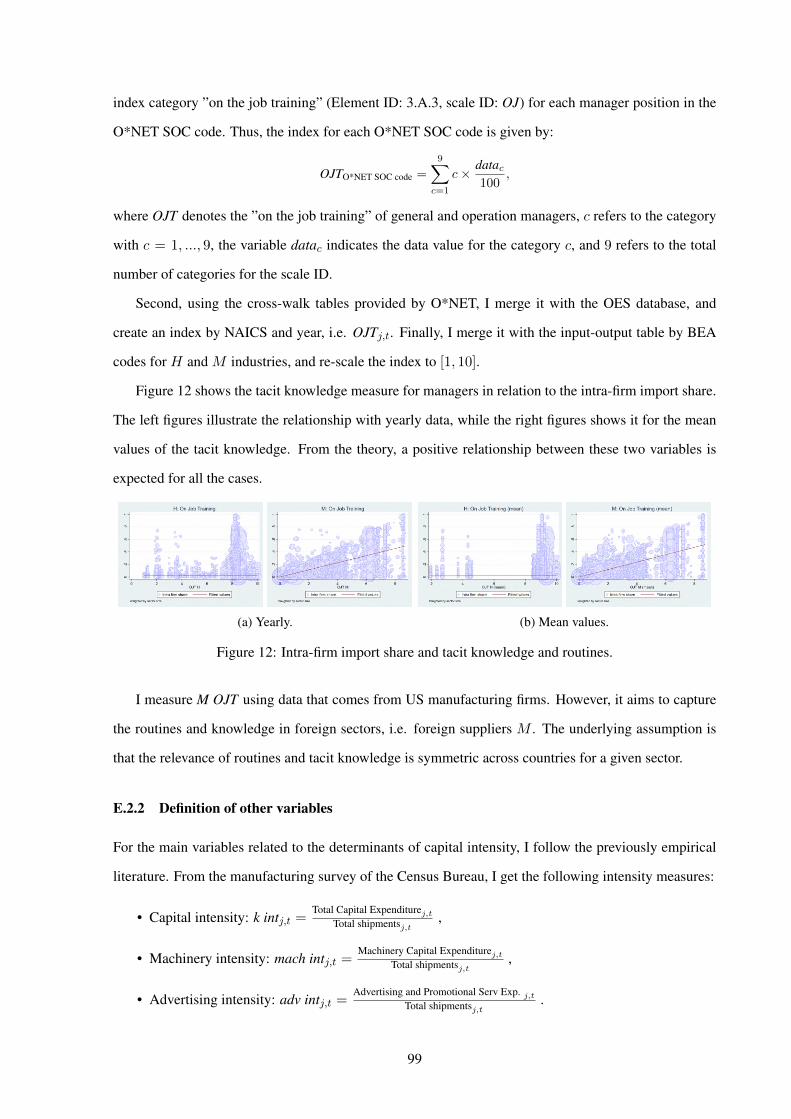
index category ”on the job training” (Element ID: 3.A.3, scale ID: OJ) for each manager position in the

O*NET SOC code. Thus, the index for each O*NET SOC code is given by:

OJTO*NET SOC code =

9∑c=1

c× datac100

,

where OJT denotes the ”on the job training” of general and operation managers, c refers to the category

with c = 1, ..., 9, the variable datac indicates the data value for the category c, and 9 refers to the total

number of categories for the scale ID.

Second, using the cross-walk tables provided by O*NET, I merge it with the OES database, and

create an index by NAICS and year, i.e. OJTj,t. Finally, I merge it with the input-output table by BEA

codes for H and M industries, and re-scale the index to [1, 10].

Figure 12 shows the tacit knowledge measure for managers in relation to the intra-firm import share.

The left figures illustrate the relationship with yearly data, while the right figures shows it for the mean

values of the tacit knowledge. From the theory, a positive relationship between these two variables is

expected for all the cases.

(a) Yearly. (b) Mean values.

Figure 12: Intra-firm import share and tacit knowledge and routines.

I measure M OJT using data that comes from US manufacturing firms. However, it aims to capture

the routines and knowledge in foreign sectors, i.e. foreign suppliers M . The underlying assumption is

that the relevance of routines and tacit knowledge is symmetric across countries for a given sector.

E.2.2 Definition of other variables

For the main variables related to the determinants of capital intensity, I follow the previously empirical

literature. From the manufacturing survey of the Census Bureau, I get the following intensity measures:

• Capital intensity: k intj,t =Total Capital Expenditurej,t

Total shipmentsj,t,

• Machinery intensity: mach intj,t =Machinery Capital Expenditurej,t

Total shipmentsj,t,

• Advertising intensity: adv intj,t =Advertising and Promotional Serv Exp. j,t

Total shipmentsj,t.

99

As robustness, I use the machinery intensity as a alternative to the total capital intensity.

The R&D intensity intensity measure is constructed from the Business R&D and Innovation Survey

(BRDIS) survey of the National Center for Science and Engineering Statistics (NCSES) of the National

Science Foundation, and it is defined as: rd intj,t =R&D Expenditurej,t

Total Salesj,t.

Figure 13 shows a linear and quadratic relationship between the H-intensity measures and the intra-

firm import share. I show also the relationship relative to the indices for ηj from a factor analysis (FA)

and a principal component analysis (PCA). The latter are illustrated in figure 14.

(a) Yearly.

(b) Mean values.

Figure 13: Component-intensity: individual measures.

(a) Yearly. (b) Mean values.

Figure 14: Intra-firm share and measures of η (FA and PCA).

E.2.3 The model

The input-out matrix structure allows me to exploit the variation across inputs-intensity and supplier’s

countries in final good producer sectors. For the construction of the variables at the final good producer

sector level, I aggregate the M -sector dimension, where the variables are weighted by the relevance of

the sector M in sector H imports according to the input-output import matrix (MshrHm,j).

100

Given the non-linear nature of the model, I estimate it by a fractional logit model, which is given by:

E[IFshrj,l,t

∣∣∣x] =exp(x′

j,l,tβ)

1 + exp(x′j,l,tβ)

, (82)

with IFshrj,l,t as the intra-firm import share from country l in year t of sector j, and

x′j,l,tβ =β1k intj,t + β2k int2j,t + β3rd intj,t + β4rd int2j,t + β5adv intj,t + β6adv int2j,t

+ β7 ln(H OJTj,t) + β8 ln(M OJTj,t) + other controls + γlt,

(83)

where H OJTj,t refers to the ”on the job training” index for managers in the final good sector j in year

t. Instead, M OJTj,t refers to the ”on the job training” index for managers for supplier industries. The

model measures it as the weighted mean of the index for each input m used by sector j. Given that both

indices are increasing in the training time, a higher OJT represents a lower δV , which translates into a

higher efficiency loss when the party that owns the assets fires the manager of the other party.

The variables identifying the H-intensity comes from the literature (Yeaple, 2006; Nunn and Trefler,

2013; Antras, 2015), and they have been defined in section E.2.2. Based on Rauch’s classification, I

include also the degree of differentiation of the supplier sectors, M diff ∈ [0, 1]. In the model, it is

defined by the weighted mean of the index for the intermediate inputs used by sector j. Additionally,

I control for the H differentiation level, with H diff ∈ [0, 1]. Finally, γlt indicates country-year fixed

effects.

For the specification with PCA or FA, the vector x is given by:

x′j,l,tβ = β1FAj,t + β2FA2

j,t + β3 ln(H OJTj,t) + β4 ln(M OJTj,t) + other controls + γlt,

x′j,l,tβ = β1PCAj,t + β2PCA2

j,t + β3 ln(H OJTj,t) + β4 ln(M OJTj,t) + other controls + γlt.

(84)

Results. The results reported in Table 8 provide evidence consistent with a non-linear U-shape rela-

tionship, as predicted by the generalised model where the property rights are allocated to the relatively

more important party on the relationship. In other words, the empirical results provide some support for

the prediction that the intra-firm import share is higher at both extremes of the ηj distribution.

Columns (1)-(8) identifies the models as defined above, while in columns (9)-(16) I introduce the

main determinants of η in mean values with the aim of capturing the underlying H technological inten-

sity. The FA measure shows a theory-consistent effect through all the specifications, while it is weaker

for the case of the PCA. Regarding the individual measures, they all show a theory-consistent effect,

except for the R&D intensity.

101

Tabl

e8:

Em

piri

cale

vide

nce

fort

hege

nera

lised

mod

elof

orga

nisa

tiona

lcho

ices

.Coe

ffici

ents

.

Det

erm

inan

tsofη j

:yea

rly

data

[col

umns

:(1)

-(8)

]D

eter

min

ants

ofη j

:mea

nda

ta[c

olum

ns:(

9)-(

16)]

(1)

(2)

(3)

(4)

(5)

(6)

(7)

(8)

(9)

(10)

(11)

(12)

(13)

(14)

(15)

(16)

IFsh

r l,j,t

IFsh

r l,j,t

IFsh

r l,j,t

IFsh

r l,j,t

IFsh

r l,j,t

IFsh

r l,j,t

IFsh

r l,j,t

IFsh

r l,j,t

IFsh

r l,j,t

IFsh

r l,j,t

IFsh

r l,j,t

IFsh

r l,j,t

IFsh

r l,j,t

IFsh

r l,j,t

IFsh

r l,j,t

IFsh

r l,j,t

PC

Aj,.

-0.0

682∗∗∗

-0.1

00∗∗∗

-0.0

251

-0.0

632∗∗∗

(0.0

225)

(0.0

222)

(0.0

213)

(0.0

211)

PC

A2 j,.

0.00

793∗∗∗

0.00

960∗∗∗

0.05

42∗∗∗

0.06

24∗∗∗

(0.0

0179

)(0

.001

72)

(0.0

0755

)(0

.007

32)

FAj,.

-0.1

25∗∗∗

-0.1

73∗∗∗

-0.1

02∗∗∗

-0.1

74∗∗∗

(0.0

319)

(0.0

314)

(0.0

301)

(0.0

301)

FA2 j,.

0.01

74∗∗∗

0.02

11∗∗∗

0.07

09∗∗∗

0.10

5∗∗∗

(0.0

0363

)(0

.003

43)

(0.0

221)

(0.0

190)

Kin

t j,.

-6.2

10∗∗∗

-7.6

81∗∗∗

-9.6

62∗

-19.

15∗∗∗

(1.9

81)

(1.9

51)

(5.6

00)

(5.5

75)

Kin

t2 j,.

28.2

4∗∗∗

33.1

3∗∗∗

100.

919

2.4∗∗∗

(9.4

87)

(9.1

82)

(64.

62)

(62.

52)

Mac

hin

t j,.

-7.7

73∗∗∗

-9.6

04∗∗∗

-13.

25∗∗

-23.

43∗∗∗

(2.1

39)

(2.0

97)

(6.4

43)

(6.4

73)

Mac

hin

t2 j,.

37.7

0∗∗∗

44.2

7∗∗∗

203.

6∗∗

317.

0∗∗∗

(10.

76)

(10.

39)

(93.

11)

(91.

33)

Adv

int j,.

-108

.2∗∗∗

-107

.9∗∗∗

-105

.3∗∗∗

-105

.0∗∗∗

-286

.8∗∗∗

-288

.6∗∗∗

-308

.0∗∗∗

-313

.4∗∗∗

(9.6

24)

(9.5

80)

(9.6

00)

(9.5

52)

(27.

00)

(26.

85)

(28.

06)

(28.

07)

Adv

int2 j,.

2474

.2∗∗∗

2486

.8∗∗∗

2374

.9∗∗∗

2390

.5∗∗∗

1667

9.2∗∗∗

1667

0.4∗∗∗

1995

0.3∗∗∗

2035

2.4∗∗∗

(309

.8)

(307

.9)

(309

.7)

(307

.8)

(363

1.1)

(362

7.1)

(377

8.3)

(379

2.1)

RD

int j

18.3

7∗∗∗

19.3

7∗∗∗

17.2

9∗∗∗

18.5

0∗∗∗

15.0

7∗∗∗

14.9

1∗∗∗

14.6

3∗∗∗

14.7

9∗∗∗

(1.9

15)

(1.9

61)

(1.9

05)

(1.9

49)

(2.0

21)

(1.9

89)

(1.9

81)

(1.9

55)

RD

int2 j

-54.

11∗∗∗

-62.

12∗∗∗

-51.

83∗∗∗

-61.

74∗∗∗

-28.

01-2

7.46

-32.

45∗

-34.

88∗∗

(16.

79)

(17.

17)

(16.

74)

(17.

09)

(17.

67)

(17.

52)

(17.

51)

(17.

41)

ln(H

OJTj,.)

-0.2

36∗∗∗

-0.2

32∗∗∗

-0.4

39∗∗∗

-0.4

36∗∗∗

-0.1

06∗

-0.1

10∗

-0.1

86∗∗∗

-0.1

94∗∗∗

-0.1

09∗

-0.1

32∗∗

-0.3

34∗∗∗

-0.3

62∗∗∗

0.06

080.

0737

-0.0

673

-0.0

583

(0.0

640)

(0.0

639)

(0.0

664)

(0.0

662)

(0.0

630)

(0.0

631)

(0.0

636)

(0.0

636)

(0.0

601)

(0.0

601)

(0.0

642)

(0.0

654)

(0.0

626)

(0.0

606)

(0.0

657)

(0.0

637)

ln(M

OJTj,.)

0.59

8∗∗∗

0.59

6∗∗∗

0.68

7∗∗∗

0.68

6∗∗∗

0.96

7∗∗∗

0.97

0∗∗∗

0.97

2∗∗∗

0.97

6∗∗∗

0.26

1∗∗∗

0.25

9∗∗∗

0.36

1∗∗∗

0.36

7∗∗∗

0.67

4∗∗∗

0.67

0∗∗∗

0.69

8∗∗∗

0.69

3∗∗∗

(0.0

441)

(0.0

442)

(0.0

446)

(0.0

447)

(0.0

464)

(0.0

464)

(0.0

460)

(0.0

460)

(0.0

315)

(0.0

320)

(0.0

336)

(0.0

341)

(0.0

331)

(0.0

329)

(0.0

333)

(0.0

331)

Hdi

ff j0.

351∗∗∗

0.32

7∗∗∗

0.47

9∗∗∗

0.45

1∗∗∗

-0.2

64∗∗∗

-0.2

48∗∗∗

-0.2

07∗∗

-0.1

86∗∗

0.11

90.

0717

0.25

7∗∗∗

0.20

6∗∗

-0.6

23∗∗∗

-0.6

09∗∗∗

-0.5

75∗∗∗

-0.5

49∗∗∗

(0.0

916)

(0.0

916)

(0.0

917)

(0.0

915)

(0.0

855)

(0.0

865)

(0.0

856)

(0.0

866)

(0.0

890)

(0.0

911)

(0.0

888)

(0.0

899)

(0.0

824)

(0.0

829)

(0.0

818)

(0.0

826)

Mdi

ff j2.

889∗∗∗

2.91

6∗∗∗

2.53

2∗∗∗

2.55

8∗∗∗

1.39

1∗∗∗

1.36

5∗∗∗

1.37

9∗∗∗

1.34

4∗∗∗

3.58

7∗∗∗

3.66

2∗∗∗

3.17

1∗∗∗

3.23

3∗∗∗

2.08

2∗∗∗

2.09

1∗∗∗

2.02

6∗∗∗

2.03

7∗∗∗

(0.1

56)

(0.1

57)

(0.1

59)

(0.1

60)

(0.1

74)

(0.1

73)

(0.1

73)

(0.1

72)

(0.1

40)

(0.1

44)

(0.1

47)

(0.1

50)

(0.1

62)

(0.1

61)

(0.1

62)

(0.1

61)

ln(s

igm

a j)

0.14

0∗∗∗

0.13

7∗∗∗

0.14

5∗∗∗

0.14

2∗∗∗

0.21

6∗∗∗

0.22

0∗∗∗

0.21

0∗∗∗

0.21

5∗∗∗

0.08

42∗∗

0.09

06∗∗∗

0.09

49∗∗∗

0.09

37∗∗∗

0.17

4∗∗∗

0.17

0∗∗∗

0.16

8∗∗∗

0.16

7∗∗∗

(0.0

321)

(0.0

320)

(0.0

307)

(0.0

305)

(0.0

277)

(0.0

280)

(0.0

280)

(0.0

283)

(0.0

328)

(0.0

329)

(0.0

315)

(0.0

313)

(0.0

282)

(0.0

286)

(0.0

282)

(0.0

286)

ln(1

+ta

riff l,j,t)

-8.8

40∗∗

-8.6

76∗∗

-11.

07∗∗∗

-10.

90∗∗∗

6.03

96.

405∗

4.00

54.

411

0.14

8-1

.574

-2.2

76-4

.254

14.4

8∗∗∗

15.0

3∗∗∗

10.8

8∗∗∗

11.7

1∗∗∗

(3.5

72)

(3.5

77)

(3.6

19)

(3.6

17)

(3.8

89)

(3.8

78)

(4.0

26)

(4.0

05)

(3.5

19)

(3.5

63)

(3.5

36)

(3.5

80)

(3.4

70)

(3.4

56)

(3.5

44)

(3.5

16)

ln(s

kill

int j

)0.

523∗∗∗

0.53

4∗∗∗

0.22

6∗∗∗

0.23

2∗∗∗

0.53

5∗∗∗

0.57

9∗∗∗

0.35

2∗∗∗

0.35

0∗∗∗

(0.0

513)

(0.0

510)

(0.0

476)

(0.0

473)

(0.0

528)

(0.0

532)

(0.0

491)

(0.0

489)

Obs

erva

tions

6097

960

979

6097

960

979

6097

960

979

6097

960

979

6097

960

979

6097

960

979

6097

960

979

6097

960

979

Fixe

def

fect

s:co

untr

y-ye

ar(lt)

.The

subi

ndex

”.”

indi

cate

st

inco

lum

ns(1

)-(8

),w

hile

inco

lum

ns(9

)-(1

6)th

ose

vari

able

sar

ein

clud

edat

thei

rres

pect

ive

mea

nva

lues

.Coe

ffici

ents

repo

rted

.Rob

usts

tand

ard

erro

rsin

pare

nthe

ses.∗p<

0.1

0,∗∗p<

0.0

5,∗∗∗p<

0.0

1.

102

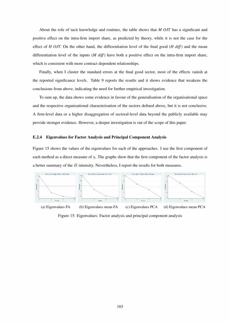
About the role of tacit knowledge and routines, the table shows that M OJT has a significant and

positive effect on the intra-firm import share, as predicted by theory, while it is not the case for the

effect of H OJT. On the other hand, the differentiation level of the final good (H diff ) and the mean

differentiation level of the inputs (M diff ) have both a positive effect on the intra-firm import share,

which is consistent with more contract dependent relationships.

Finally, when I cluster the standard errors at the final good sector, most of the effects vanish at

the reported significance levels. Table 9 reports the results and it shows evidence that weakens the

conclusions from above, indicating the need for further empirical investigation.

To sum up, the data shows some evidence in favour of the generalisation of the organisational space

and the respective organisational characterisation of the sectors defined above, but it is not conclusive.

A firm-level data or a higher disaggregation of sectoral-level data beyond the publicly available may

provide stronger evidence. However, a deeper investigation is out of the scope of this paper.

E.2.4 Eigenvalues for Factor Analysis and Principal Component Analysis

Figure 15 shows the values of the eigenvalues for each of the approaches. I use the first component of

each method as a direct measure of η. The graphs show that the first component of the factor analysis is

a better summary of the H-intensity. Nevertheless, I report the results for both measures.

(a) Eigenvalues FA (b) Eigenvalues mean FA (c) Eigenvalues PCA (d) Eigenvalues mean PCA

Figure 15: Eigenvalues: Factor analysis and principal component analysis

103

Tabl

e9:

Em

piri

cale

vide

nce

fort

hege

nera

lised

mod

elof

orga

nisa

tiona

lcho

ices

.Clu

ster

s.e.

atse

ctorj.

Coe

ffici

ents

.

Det

erm

inan

tsofη j

:yea

rly

data

[col

umns

:(1)

-(8)

]D

eter

min

ants

ofη j

:mea

nda

ta[c

olum

ns:(

9)-(

16)]

(1)

(2)

(3)

(4)

(5)

(6)

(7)

(8)

(9)

(10)

(11)

(12)

(13)

(14)

(15)

(16)

IFsh

r l,j,t

IFsh

r l,j,t

IFsh

r l,j,t

IFsh

r l,j,t

IFsh

r l,j,t

IFsh

r l,j,t

IFsh

r l,j,t

IFsh

r l,j,t

IFsh

r l,j,t

IFsh

r l,j,t

IFsh

r l,j,t

IFsh

r l,j,t

IFsh

r l,j,t

IFsh

r l,j,t

IFsh

r l,j,t

IFsh

r l,j,t

PC

Aj,.

-0.0

682

-0.1

00-0

.025

1-0

.063

2(0

.104

)(0

.097

6)(0

.103

)(0

.099

3)

PC

A2 j,.

0.00

793

0.00

960∗

0.05

42∗∗

0.06

24∗∗∗

(0.0

0602

)(0

.005

76)

(0.0

216)

(0.0

211)

FAj,.

-0.1

25-0

.173

-0.1

02-0

.174

(0.1

55)

(0.1

42)

(0.1

65)

(0.1

57)

FA2 j,.

0.01

740.

0211∗

0.07

090.

105∗∗

(0.0

123)

(0.0

116)

(0.0

503)

(0.0

478)

Kin

t j,.

-6.2

10-7

.681

-9.6

62-1

9.15∗

(4.7

45)

(4.9

21)

(10.

07)

(10.

57)

Kin

t2 j,.

28.2

4∗33

.13∗

100.

919

2.4

(16.

69)

(17.

74)

(114

.2)

(118

.5)

Mac

hin

t j,.

-7.7

73-9

.604

-13.

25-2

3.43∗

(5.7

89)

(5.9

44)

(11.

89)

(12.

45)

Mac

hin

t2 j,.

37.7

0∗44

.27∗∗

203.

631

7.0∗

(21.

36)

(22.

42)

(160

.4)

(163

.8)

Adv

int j,.

-108

.2∗∗∗

-107

.9∗∗∗

-105

.3∗∗∗

-105

.0∗∗∗

-286

.8∗∗∗

-288

.6∗∗∗

-308

.0∗∗∗

-313

.4∗∗∗

(28.

72)

(28.

36)

(25.

73)

(25.

29)

(65.

24)

(63.

61)

(70.

14)

(68.

92)

Adv

int2 j,.

2474

.2∗∗∗

2486

.8∗∗∗

2374

.9∗∗∗

2390

.5∗∗∗

1667

9.2∗∗

1667

0.4∗∗

1995

0.3∗∗

2035

2.4∗∗∗

(726

.6)

(725

.1)

(633

.1)

(630

.5)

(720

7.2)

(703

6.4)

(792

4.6)

(783

4.3)

RD

int j

18.3

7∗∗∗

19.3

7∗∗∗

17.2

9∗∗∗

18.5

0∗∗∗

15.0

7∗∗∗

14.9

1∗∗∗

14.6

3∗∗∗

14.7

9∗∗∗

(3.8

25)

(3.8

56)

(3.9

76)

(3.8

49)

(3.6

03)

(3.6

15)

(3.6

36)

(3.6

16)

RD

int2 j

-54.

11∗

-62.

12∗∗

-51.

83∗

-61.

74∗∗

-28.

01-2

7.46

-32.

45-3

4.88

(28.

79)

(28.

23)

(29.

43)

(28.

10)

(30.

38)

(29.

42)

(29.

57)

(28.

94)

ln(H

OJTj,.)

-0.2

36-0

.232

-0.4

39∗

-0.4

36∗

-0.1

06-0

.110

-0.1

86-0

.194

-0.1

09-0

.132

-0.3

34-0

.362

0.06

080.

0737

-0.0

673

-0.0

583

(0.2

24)

(0.2

26)

(0.2

47)

(0.2

45)

(0.1

15)

(0.1

16)

(0.1

24)

(0.1

26)

(0.2

17)

(0.2

52)

(0.2

46)

(0.2

67)

(0.1

39)

(0.1

29)

(0.1

31)

(0.1

24)

ln(M

OJTj,.)

0.59

8∗∗∗

0.59

6∗∗∗

0.68

7∗∗∗

0.68

6∗∗∗

0.96

7∗∗∗

0.97

0∗∗∗

0.97

2∗∗∗

0.97

6∗∗∗

0.26

1∗0.

259∗

0.36

1∗∗∗

0.36

7∗∗∗

0.67

4∗∗∗

0.67

0∗∗∗

0.69

8∗∗∗

0.69

3∗∗∗

(0.1

63)

(0.1

63)

(0.1

25)

(0.1

26)

(0.1

07)

(0.1

08)

(0.0

977)

(0.0

989)

(0.1

46)

(0.1

46)

(0.1

07)

(0.1

09)

(0.0

881)

(0.0

866)

(0.0

810)

(0.0

808)

Hdi

ff j0.

351

0.32

70.

479

0.45

1-0

.264

-0.2

48-0

.207

-0.1

860.

119

0.07

170.

257

0.20

6-0

.623∗∗

-0.6

09∗∗

-0.5

75∗∗

-0.5

49∗∗

(0.4

80)

(0.4

91)

(0.4

24)

(0.4

29)

(0.3

18)

(0.3

09)

(0.2

87)

(0.2

80)

(0.4

61)

(0.4

80)

(0.4

03)

(0.4

13)

(0.2

78)

(0.2

72)

(0.2

33)

(0.2

33)

Mdi

ff j2.

889∗∗∗

2.91

6∗∗∗

2.53

2∗∗∗

2.55

8∗∗∗

1.39

1∗∗∗

1.36

5∗∗∗

1.37

9∗∗∗

1.34

4∗∗∗

3.58

7∗∗∗

3.66

2∗∗∗

3.17

1∗∗∗

3.23

3∗∗∗

2.08

2∗∗∗

2.09

1∗∗∗

2.02

6∗∗∗

2.03

7∗∗∗

(0.6

70)

(0.6

80)

(0.4

86)

(0.4

93)

(0.3

78)

(0.3

74)

(0.3

42)

(0.3

40)

(0.6

58)

(0.6

84)

(0.4

72)

(0.4

86)

(0.3

40)

(0.3

38)

(0.3

01)

(0.3

05)

ln(s

igm

a j)

0.14

00.

137

0.14

50.

142

0.21

6∗∗∗

0.22

0∗∗∗

0.21

0∗∗∗

0.21

5∗∗∗

0.08

420.

0906

0.09

490.

0937

0.17

4∗∗∗

0.17

0∗∗∗

0.16

8∗∗∗

0.16

7∗∗∗

(0.1

16)

(0.1

16)

(0.0

981)

(0.0

967)

(0.0

726)

(0.0

727)

(0.0

682)

(0.0

682)

(0.1

16)

(0.1

19)

(0.1

02)

(0.1

03)

(0.0

596)

(0.0

598)

(0.0

535)

(0.0

548)

ln(1

+ta

riff l,j,t)

-8.8

40-8

.676

-11.

07∗

-10.

90∗

6.03

96.

405

4.00

54.

411

0.14

8-1

.574

-2.2

76-4

.254

14.4

8∗∗∗

15.0

3∗∗∗

10.8

8∗∗

11.7

1∗∗∗

(7.5

96)

(7.5

93)

(6.3

23)

(6.2

60)

(5.1

73)

(5.1

96)

(4.8

38)

(4.8

20)

(7.6

61)

(8.1

06)

(6.4

72)

(6.8

77)

(4.9

90)

(4.9

34)

(4.6

64)

(4.5

43)

ln(s

kill

int j

)0.

523∗∗

0.53

4∗∗

0.22

60.

232

0.53

5∗∗

0.57

9∗∗

0.35

2∗∗∗

0.35

0∗∗∗

(0.2

56)

(0.2

52)

(0.1

53)

(0.1

53)

(0.2

65)

(0.2

68)

(0.1

23)

(0.1

26)

Obs

erva

tions

6097

960

979

6097

960

979

6097

960

979

6097

960

979

6097

960

979

6097

960

979

6097

960

979

6097

960

979

Fixe

def

fect

s:co

untr

y-ye

ar(lt)

.The

subi

ndex

”.”

indi

cate

st

inco

lum

ns(1

)-(8

),w

hile

inco

lum

ns(9

)-(1

6)th

eyar

ein

clud

edat

mea

nva

lues

.Clu

ster

s.e.

atfin

algo

odse

ctorj.

Coe

ffici

ents

repo

rted

.Sta

ndar

der

rors

inpa

rent

hese

s.∗p<

0.1

0,∗∗p<

0.0

5,∗∗∗p<

0.0

1

104

E.3 Empirical dynamic model

E.3.1 Derivation of total imports and offshoring share: sectoral aggregate.

I compute the aggregate imports of sector j under outsourcing in period t:

XSm,O,j,t =

∫ θV,j,t

θO,j,t

xSm,O,j,t(θ)Hj,tg(θ)

1−G(θj,t)dθ

=Hj,t

[χSO,j,t

∫ ∞θSO,j,t

xSm,O,j,t(θ)g(θ)

1−G(θSO,j,t)dθ − χSV,j,t

∫ ∞θSV,j,t

xSm,O,j,t(θ)g(θ)

1−G(θSV,j,t)dθ

]

=Hj,tασjj (1− βj)(1− ηj)

wSγjEP

σj−1

j,t

[(βSjwN

)ηj (1− βSjwS

)1−ηj]σj−1

×[χSO,j,t

(θSO,j,t

)σj−1

− χSV,j,t(θSV,j,t

)σj−1]

(85)

Adding (97) and (85), I obtain the aggregate total imports of sector j in period t:

XSm,j,t =XS

m,O,j,t +XSm,V,j,t,

=Hj,t[χSO,j,tx

Sm,O,j,t(θ

SO,j,t) + χSV,j,t

[xSm,V,j,t(θ

SV,j,t)− xSm,O,j,t(θSO,j,t)

]].

(86)

UsingxSm,V,j,t(θ)

xSm,O,j,t(θ)=

1−βSV,j,t1−βj

[(βSV,j,tβj

)ηj (1−βSV,j,t1−βj

)1−ηj]σj−1

, I get:

XSm,j,t =Hj,t

χSO,j,txSm,O,j,t(θSO,j,t) + χSV,j,t

1− βSV,j,t1− βj

[(βSV,j,tβj

)ηj (1− βSV,j,t

1− βj

)1−ηj]σj−1

− 1

xSm,O,j,t(θSO,j,t) .

(87)

Replacing with the respective expressions for xm,.,j,t(.):

XSm,j,t =Hj,t

ασjj (1− βj)(1− ηj)

wSγjEP

σj−1

j,t

[(βSjwN

)ηj (1− βSjwS

)1−ηj]σj−1

×

χSO,j,t(θSO,j,t)σj−1 + χSV,j,t

1− βSV,j,t1− βj

[(βSV,j,tβj

)ηj (1− βSV,j,t

1− βj

)1−ηj]σj−1

− 1

(θSV,j,t)σj−1

(88)

The offshoring share of sector j in period t is:

offshr shrj,t ≡wSXS

m,j,t

γjE

=Hj,tασjj (1− βj)(1− ηj)P

σj−1

j,t

[(βSjwN

)ηj (1− βSjwS

)1−ηj]σj−1

×

χSO,j,t(θSO,j,t)σj−1 + χSV,j,t

1− βSV,j,t1− βj

[(βSV,j,tβj

)ηj (1− βSV,j,t

1− βj

)1−ηj]σj−1

− 1

(θSV,j,t)σj−1

(89)

E.3.2 Competition effect: first channel. Reduced-form models

Table 10 reports the full table related to the results in Table 1, and additional robustness checks. In

particular, it includes the estimation results of the effect of the offshoring share in levels on the intra-firm

import share. The table reports the estimated coefficients and the average marginal effects.

105

Table 10: Competition effect: full table.

(1) (2) (3)IFshrj,t IFshrj,t IFintj,t

+ ++ + ++ + ++ln(offshr shrj,t) -0.180∗∗ -0.0381∗∗∗

(0.0768) (0.0139)

offshr shrj,t -2.356∗ -0.506∗ 11.69∗∗∗ 0.279∗∗∗

(1.427) (0.289) (1.319) (0.0389)

offshr shr2j,t -6.006∗∗∗ -0.143∗∗∗

(1.268) (0.0331)

H diffj 0.806 0.171 0.728 0.156 1.417∗∗∗ 0.0338∗∗∗

(0.797) (0.176) (0.926) (0.204) (0.447) (0.0118)

M diffj 1.970∗∗∗ 0.417∗∗∗ 1.966∗∗ 0.422∗∗∗ 1.665∗∗∗ 0.0398∗∗∗

(0.715) (0.123) (0.766) (0.136) (0.594) (0.0126)

ln(sigmaj) 0.599∗∗ 0.127∗∗ 0.614∗ 0.132∗∗ 0.547∗∗∗ 0.0131∗∗∗

(0.295) (0.0545) (0.342) (0.0657) (0.162) (0.00368)

η(FA)j -0.477 -0.101 -0.504 -0.108 -0.501∗∗∗ -0.0120∗∗∗

(0.340) (0.0647) (0.381) (0.0741) (0.192) (0.00409)

constant -3.893∗∗∗ -2.940∗∗∗ -8.357∗∗∗

(0.877) (0.866) (0.407)FEs t t t t t t

Observations 2039 2039 2039 2039 2039 2039Coefficients (+) and average marginal effects (++). Standard errors in parentheses. Cluster s.e. at sector j.∗ p < 0.10, ∗∗ p < 0.05, ∗∗∗ p < 0.01

Table 11 shows the estimated coefficients and the average marginal effects of the models reported in

Table 10, but including final good producer sector fixed effects.

Table 11: Competition effect: sector j FEs.

(1) (2) (3)IFshrj,t IFshrj,t IFintj,t

+ ++ + ++ + ++

ln(offshr shrj,t) 0.0450∗ 0.00797∗

(0.0238) (0.00421)

offshr shrj,t -0.141 -0.0251 16.69∗∗∗ 0.393∗∗∗

(0.562) (0.0996) (2.007) (0.0471)

offshr shr2j,t -13.38∗∗∗ -0.315∗∗∗

(2.215) (0.0522)FEs t , j t , j t , jObservations 2078 2078 2078Coefficients (+) and average marginal effects (++). Standard errors in parentheses∗ p < 0.10, ∗∗ p < 0.05, ∗∗∗ p < 0.01

106

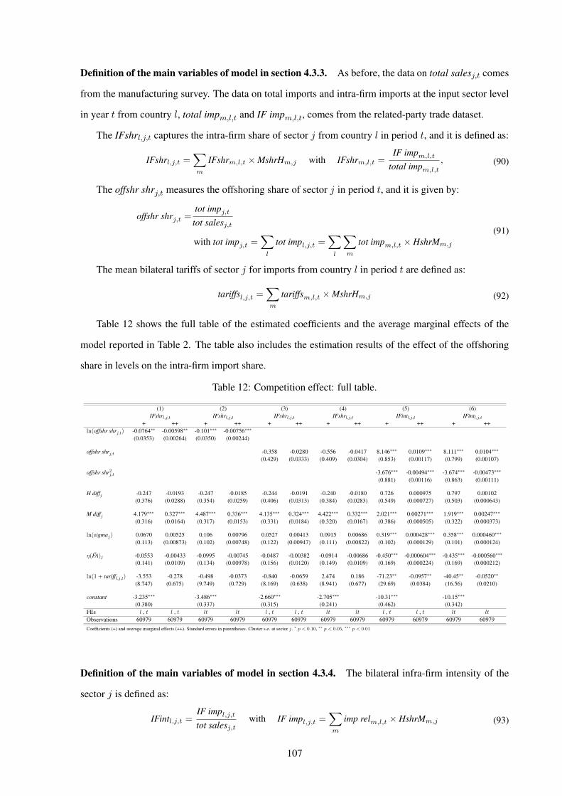
Definition of the main variables of model in section 4.3.3. As before, the data on total salesj,t comes

from the manufacturing survey. The data on total imports and intra-firm imports at the input sector level

in year t from country l, total impm,l,t and IF impm,l,t, comes from the related-party trade dataset.

The IFshrl,j,t captures the intra-firm share of sector j from country l in period t, and it is defined as:

IFshrl,j,t =∑m

IFshrm,l,t ×MshrHm,j with IFshrm,l,t =IF impm,l,t

total impm,l,t, (90)

The offshr shrj,t measures the offshoring share of sector j in period t, and it is given by:

offshr shrj,t =tot impj,t

tot salesj,t

with tot impj,t =∑l

tot impl,j,t =∑l

∑m

tot impm,l,t × HshrMm,j

(91)

The mean bilateral tariffs of sector j for imports from country l in period t are defined as:

tariffsl,j,t =∑m

tariffsm,l,t ×MshrHm,j (92)

Table 12 shows the full table of the estimated coefficients and the average marginal effects of the

model reported in Table 2. The table also includes the estimation results of the effect of the offshoring

share in levels on the intra-firm import share.

Table 12: Competition effect: full table.

(1) (2) (3) (4) (5) (6)IFshrl,j,t IFshrl,j,t IFshrl,j,t IFshrl,j,t IFintl,j,t IFintl,j,t

+ ++ + ++ + ++ + ++ + ++ + ++ln(offshr shrj,t) -0.0764∗∗ -0.00598∗∗ -0.101∗∗∗ -0.00756∗∗∗

(0.0353) (0.00264) (0.0350) (0.00244)

offshr shrj,t -0.358 -0.0280 -0.556 -0.0417 8.146∗∗∗ 0.0109∗∗∗ 8.111∗∗∗ 0.0104∗∗∗

(0.429) (0.0333) (0.409) (0.0304) (0.853) (0.00117) (0.799) (0.00107)

offshr shr2j,t -3.676∗∗∗ -0.00494∗∗∗ -3.674∗∗∗ -0.00473∗∗∗

(0.881) (0.00116) (0.863) (0.00111)

H diffj -0.247 -0.0193 -0.247 -0.0185 -0.244 -0.0191 -0.240 -0.0180 0.726 0.000975 0.797 0.00102(0.376) (0.0288) (0.354) (0.0259) (0.406) (0.0313) (0.384) (0.0283) (0.549) (0.000727) (0.503) (0.000643)

M diffj 4.179∗∗∗ 0.327∗∗∗ 4.487∗∗∗ 0.336∗∗∗ 4.135∗∗∗ 0.324∗∗∗ 4.422∗∗∗ 0.332∗∗∗ 2.021∗∗∗ 0.00271∗∗∗ 1.919∗∗∗ 0.00247∗∗∗

(0.316) (0.0164) (0.317) (0.0153) (0.331) (0.0184) (0.320) (0.0167) (0.386) (0.000505) (0.322) (0.000373)

ln(sigmaj) 0.0670 0.00525 0.106 0.00796 0.0527 0.00413 0.0915 0.00686 0.319∗∗∗ 0.000428∗∗∗ 0.358∗∗∗ 0.000460∗∗∗

(0.113) (0.00873) (0.102) (0.00748) (0.122) (0.00947) (0.111) (0.00822) (0.102) (0.000129) (0.101) (0.000124)

η(FA)j -0.0553 -0.00433 -0.0995 -0.00745 -0.0487 -0.00382 -0.0914 -0.00686 -0.450∗∗∗ -0.000604∗∗∗ -0.435∗∗∗ -0.000560∗∗∗

(0.141) (0.0109) (0.134) (0.00978) (0.156) (0.0120) (0.149) (0.0109) (0.169) (0.000224) (0.169) (0.000212)

ln(1 + tariffl,j,t) -3.553 -0.278 -0.498 -0.0373 -0.840 -0.0659 2.474 0.186 -71.23∗∗ -0.0957∗∗ -40.45∗∗ -0.0520∗∗

(8.747) (0.675) (9.749) (0.729) (8.169) (0.638) (8.941) (0.677) (29.69) (0.0384) (16.56) (0.0210)

constant -3.235∗∗∗ -3.486∗∗∗ -2.660∗∗∗ -2.705∗∗∗ -10.31∗∗∗ -10.15∗∗∗

(0.380) (0.337) (0.315) (0.241) (0.462) (0.342)FEs l , t l , t lt lt l , t l , t lt lt l , t l , t lt lt

Observations 60979 60979 60979 60979 60979 60979 60979 60979 60979 60979 60979 60979Coefficients (+) and average marginal effects (++). Standard errors in parentheses. Cluster s.e. at sector j. ∗ p < 0.10, ∗∗ p < 0.05, ∗∗∗ p < 0.01

Definition of the main variables of model in section 4.3.4. The bilateral infra-firm intensity of the

sector j is defined as:

IFintl,j,t =IF impl,j,ttot salesj,t

with IF impl,j,t =∑m

imp relm,l,t × HshrMm,j (93)

107

Table 13 shows that that the offshoring activity has an opposite effect on the intra-firm import share

relative to the theoretical predictions, when ρj fixed effects are included. In the case of the models related

to the effects on the intra-firm intensity, the results and conclusions remain robust in all the specifications.

Table 13: Competition effect: sector j FEs.

(1) (2) (3) (4) (5) (6)IFshrl,j,t IFshrl,j,t IFshrl,j,t IFshrl,j,t IFintl,j,t IFintl,j,t

+ ++ + ++ + ++ + ++ + ++ + ++

ln(offshr shrj,t) 0.0388∗∗ 0.00300∗∗ 0.0389∗ 0.00287∗

(0.0188) (0.00145) (0.0236) (0.00174)

offshr shrj,t 0.948∗∗∗ 0.0731∗∗∗ 1.031∗∗∗ 0.0761∗∗∗ 6.469∗∗∗ 0.00865∗∗∗ 7.799∗∗∗ 0.00999∗∗∗

(0.279) (0.0214) (0.375) (0.0271) (0.891) (0.00131) (0.574) (0.000746)

offshr shr2j,t -2.957∗∗∗ -0.00396∗∗∗ -4.000∗∗∗ -0.00512∗∗∗

(0.800) (0.00111) (0.594) (0.000761)

ln(1 + tariffl,j,t) 19.77∗∗ 1.527∗∗ 30.65∗∗∗ 2.263∗∗∗ 20.64∗∗ 1.593∗∗ 31.97∗∗∗ 2.359∗∗∗ -73.86∗∗ -0.0988∗∗ -39.32∗ -0.0504∗

(8.635) (0.669) (7.469) (0.554) (8.236) (0.638) (7.069) (0.523) (34.04) (0.0453) (21.51) (0.0279)FEs j , l , t j , lt j , l , t j , lt j , l , t j , ltObservations 62188 62188 62188 62188 62188 62188Coefficients (+) and average marginal effects (++). Standard errors in parentheses. Cluster s.e. at sector j. ∗ p < 0.10, ∗∗ p < 0.05, ∗∗∗ p < 0.01

E.3.3 Competition effect: First channel. Derivation of first and second stages

First stage: Price index. The sector’s price index can be expressed as:115

P1−σjj,t =

(PONj,tj,t

)1−σj+ χNV,j,t

[(PV Nj,tj,t

)1−σj−(PV Nj,t|O

Nj,t

j,t

)1−σj]

+ χSO,j,t

[(POSj,tj,t

)1−σj−(POSj,t|V

Nj,t

j,t

)1−σj]

+ χSV,j,t

[(PV Sj,tj,t

)1−σj−(PV Sj,t|O

Sj,t

j,t

)1−σj],

(94)

where Pklj,tj,t represents the price index of all the producers θ ≥ θlk,j,t in sector j as if they were all under

organisational structure kl. Finally, POSj,t|V Nj,tj,t denotes the price index of all the producers θ ≥ θSO,j,t as if

they were under the cost structure of domestic integration, and PV Sj,t|OSj,tj,t refers to the price index of all

the producers θ ≥ θSV,j,t as if they were under the cost structure of foreign outsourcing.

As already mentioned, χSO,j,t indicates the share of final good producers under any type of offshoring

in t. Equation (94) shows that as more final good producers offshore, i.e. χSO,j,t ↑, the lower the price in-

dex.116 In the empirical model, I proxy the changes in the extensive margin of final good producers under

offshoring, χSO,j,t, by changes in the offshoring intensive margin at the sectoral level, i.e. offshr shrj,t.

The first-stage regression is thus given by:

ln(Pj,t) = b0 + b1 ln(offshr shrj,t) + other controls + bl + bt + uj,t

115See Appendix A.8 for proofs.116An increase in χSO,j,t generates a reduction in χSV,j,t, χ

SV,j,t and an increase in the market productivity cutoff. While

the latter generates a further reduction in the price index, due to the higher mean productivity in the market, the verticaldisintegration in the domestic and offshore supply chains induce an increase in the price index. However, those effects comefrom the initial reduction in the price index. Therefore, it is easy to see that those effects do not overcome the initial impact,and thus the increase in χSO,j,t has a negative net effect on the price index.

108

Second stage: Intra-firm intensity. From the theoretical model above, I have that intermediate input

imports in period t for a final good producer θ under foreign integration, xSm,V,j,t(θ), are given by:

xSm,V,j,t(θ) =αj(1− βSV )(1− ηj)

wSrSV,j,t(θ), (95)

with

rSV,j,t(θ) = ασj−1j θσj−1(γjE)σjQ

1−σjj,t

(βSV,jwN

)ηj (1− βSV,jwS

)1−ηjσj . (96)

Plugging (96) into (95), and replacing Qj,t =γjEPj,t

, I get:

xSm,V,j,t(θ) =ασjj (1− βSV )(1− ηj)

wSγjEP

σj−1j,t

(βSV,jwN

)ηj (1− βSV,jwS

)1−ηjσj . (97)

If I aggregate over all firms under V S in period t, the intra-firm imports in sector j in period t are:

XSm,V,j,t =

∫ ∞θV,j,t

xSm,V,j,t(θ)Hj,tg(θ)

1−G(θj,t)dθ.

The intra-firm intensity of sector j in period t is defined as IFintj,t ≡wSXS

m,V,j,t

γjE. Replacing with

(97), I get the IFintj,t as a function of Pj,t:

IFintj,t =ασjj (1− βSV,j)(1− ηj)

(βSV,jwN

)ηj (1− βSV,jwS

)1−ηjσj−1

Pσj−1j,t

[θSV,j,t

]σj−1χSV,j,tHj,t

with θSV,j,t(Pj,t), χSV,j,t(Pj,t), andHj,t(Pj,t). Taking logs and grouping all variables that depend on (Pj,t),

the intra-firm intensity is given by:

IFintj,t = exp

ln

ασjj (1− βSV,j)(1− ηj)

(βSV,jwNt

)ηj (1− βSV,jwSt

)1−ηjσj−1

+ ln [Pj,t]

, (98)

with Pj,t ≡ Pσj−1j,t

[θSV,j,t(Pj,t)

]σj−1 [χSV,j,t(Pj,t)

]σj−1[Hj,t(Pj,t)]

σj−1.

The second-stage regression is given by:

E[IFintl,j,t

∣∣∣x] =exp(x′

l,j,tρ)

1 + exp(x′l,j,tρ)

with x′l,j,tρ =ρ1

ln(Pj,t) + other controls + ρl + ρt.

From the expression of Pj,t, it is possible to see that changes in the price index have direct impacts

on the IFintj,t, as well as indirect impacts through the effects of the price index on θSV,j,t, χSV,j,t and Hj,t.

Therefore, the second stage captures the net effect of the changes in the predicted price index, i.e. the

effect of Pj,t on the intra-firm intensity due to a reduction in the offshoring productivity cutoff.

Competition effect: First channel. Two-stage regression. Tables. Table 14 reports the full table of

the first stage shown in Table 4.

109

Table 14: All first stage coefficients of table 4.

First stage: All coefficients(1) (2) (3)

ln(Pj,t) ln(Pj,t) ln(Pj,t)

ln(offshr shrj,t) -0.0312∗∗∗ -0.0350∗∗∗ -0.0352∗∗∗

(0.00869) (0.00959) (0.00979)

ln(1 + tariffl,j,t) 2.797 2.655(1.859) (1.899)

H diffj 0.0423 0.0923 0.0929(0.152) (0.151) (0.152)

M diffj -0.00168 0.0351 0.0376(0.0683) (0.0583) (0.0596)

ln(sigmaj) 0.0704 0.0788 0.0790(0.0468) (0.0499) (0.0504)

η(FA)j 0.00825 -0.00564 -0.00564(0.0227) (0.0253) (0.0255)

FEs t l , t ltR2 0.292 0.297 0.309Adjusted R2 0.285 0.294 0.282Cluster s.e. at sector j. Standard errors in parentheses.∗ p < 0.10, ∗∗ p < 0.05, ∗∗∗ p < 0.01

E.3.4 Competition effect: Both channels. Derivation of first and second stages.

First stage: Price index. The sector’s price index can be expressed as:117

P 1−σt =

(PONtt

)1−σ+ χNV,t

[(PV Ntt

)1−σ−(PV Nt |O

Nt

t

)1−σ]+ χSO,t

[(POStt

)1−σ−(POSt |V

Nt

t

)1−σ]+ χSV,t

[(PV Stt

)1−σ−(PV St |O

St

t

)1−σ]+ χEO,t

[(POEtt

)1−σ−(POEt |V

St

t

)1−σ]+ χEV,t

[(PV Ett

)1−σ−(PV Et |O

Et

t

)1−σ].

(99)

Second stage: Intra-firm intensity. The intra-firm intensity of sector j in period t is given by:

IFintl,j,t = exp

ln

ασjj (1− βlV,j)(1− ηj)

(βlV,jwNt

)ηj (1− βlV,jwlt

)1−ηjσj−1

+ ln [Pj,t]

, (100)

with Pj,t ≡ Pσj−1j,t

[θlV,j,t(Pj,t)

]σj−1 [χlV,j,t(Pj,t)

]σj−1[Hj,t(Pj,t)]

σj−1.

117See Appendix D for proofs.

110

Competition effect: Both channels. Two-stage regression. Tables. Table 15 reports the full table for

the two stages.

Table 15: Two-stage regression: Full table.

Second stage: All coefficients reportedAgg. countries No aggregation of countries

(1) (2) (3)IFintj,t IFintl,j,t IFintl,j,t

ln(Pj,t) -33.52∗∗∗ -23.42∗∗∗ -23.38∗∗∗

(1.981) (1.751) (1.697)

ln(1 + tariffl,j,t) 53.39∗∗ 61.62∗∗∗

(21.015) (19.087)

H diffj 2.158∗∗∗ 2.862∗∗∗ 2.902∗∗∗

(0.626) (0.548) (0.534)

M diffj -0.122 3.639∗∗∗ 3.557∗∗∗

(0.668) (0.582) (0.526)

ln(sigmaj) 2.263∗∗∗ 1.873∗∗∗ 1.873∗∗∗

(0.217) (0.152) (0.154)

η(FA)j 0.100 -0.405∗∗ -0.386∗∗

(0.118) (0.184) (0.174)FEs t t , l lt

First stage: All coefficients(1) (2) (3)

ln(Pj,t) ln(Pj,t) ln(Pj,t)

ln(offshr shrj,t) -0.0307∗∗∗ -0.0340∗∗∗ -0.0340∗∗∗

(0.00841) (0.00961) (0.00981)

ln(CHN mrkt shrj,t) -0.00531 -0.00784∗∗ -0.00826∗∗

(0.00332) (0.00323) (0.00343)

H diffj 0.0315 0.0957 0.0963(0.149) (0.152) (0.153)

M diffj 0.0346 0.0790 0.0816(0.0763) (0.0668) (0.0686)

ln(sigmaj) 0.0647 0.0802 0.0805(0.0448) (0.0505) (0.0510)

η(FA)j 0.00584 -0.00746 -0.00742(0.0234) (0.0259) (0.0261)

ln(1 + tariffl,j,t) 4.138∗∗ 4.119∗∗

(1.685) (1.709)FEs t t , l ltR2 0.299 0.301 0.314Adjusted R2 0.291 0.298 0.285Second stage: Bootstrapped s.e. (1000 rep). Coefficients reported.

All stages: Cluster s.e. at sector j. Standard errors in parentheses.∗ p < 0.10, ∗∗ p < 0.05, ∗∗∗ p < 0.01

111

Contents

1 Introduction 1

2 The two-country model: North-South 9

2.1 Organisational choice under perfect information. . . . . . . . . . . . . . . . . . . . . . . . . . . 10

2.2 Perfect information steady-state. . . . . . . . . . . . . . . . . . . . . . . . . . . . . . . . . . . . 14

3 Uncertainty in organisational fixed costs in South: model setup 16

3.1 Model setup and initial conditions. . . . . . . . . . . . . . . . . . . . . . . . . . . . . . . . . . . 16

3.1.1 Informational externalities and learning. . . . . . . . . . . . . . . . . . . . . . . . . . . . 18

3.1.2 Exploration decision of the offshoring potential. . . . . . . . . . . . . . . . . . . . . . . 20

3.2 Sectoral equilibrium paths. . . . . . . . . . . . . . . . . . . . . . . . . . . . . . . . . . . . . . . 22

3.2.1 H- and M -intensive sectors: The trade-off function. . . . . . . . . . . . . . . . . . . . . 22

3.2.2 H- and M -intensive sectors: Long-run properties of the trade-off function. . . . . . . . . 24

3.2.3 H- and M -intensive sectors: Competition effect and the disintegration dynamics. . . . . . 25

4 Empirical model: Competition effect in North-South model 27

4.1 Data. . . . . . . . . . . . . . . . . . . . . . . . . . . . . . . . . . . . . . . . . . . . . . . . . . . 28

4.2 Stylised facts. . . . . . . . . . . . . . . . . . . . . . . . . . . . . . . . . . . . . . . . . . . . . . 29

4.3 Identification of the empirical models and estimation results. . . . . . . . . . . . . . . . . . . . . 30

4.3.1 Reduced form model: First channel of competition effect in a two-countries setup. . . . . 31

4.3.2 Reduced form model: Intra-firm intensity. . . . . . . . . . . . . . . . . . . . . . . . . . . 33

4.3.3 Reduced form model: Competition effect at bilateral levels. . . . . . . . . . . . . . . . . 34

4.3.4 Reduced form model: Intra-firm intensity. . . . . . . . . . . . . . . . . . . . . . . . . . . 35

4.3.5 Reduced form models: Bilateral and global effects. . . . . . . . . . . . . . . . . . . . . . 35

4.3.6 Empirical model: Identification of the competition effect mechanism. . . . . . . . . . . . 36

5 Multiple countries 38

5.1 Perfect information equilibrium. . . . . . . . . . . . . . . . . . . . . . . . . . . . . . . . . . . . 38

5.2 Institutional reform in East: Model setup and initial conditions. . . . . . . . . . . . . . . . . . . . 39

5.3 Exploration decision of offshoring potential in East: Relocation and competition. . . . . . . . . . 39

5.4 Empirical model: Competition effect in multi-country model. . . . . . . . . . . . . . . . . . . . . 42

5.4.1 China access to WTO: stylized facts. . . . . . . . . . . . . . . . . . . . . . . . . . . . . . 42

5.4.2 Competition effect: China institutional shock and relocation channel. . . . . . . . . . . . 43

6 The role of FTAs and MAs on exploration decisions 45

6.1 Role of FTAs. . . . . . . . . . . . . . . . . . . . . . . . . . . . . . . . . . . . . . . . . . . . . . 45

6.1.1 Role of FTAs: tariff dimension. . . . . . . . . . . . . . . . . . . . . . . . . . . . . . . . 45

112

6.1.2 Role of FTAs: institutional dimension. . . . . . . . . . . . . . . . . . . . . . . . . . . . . 47

6.2 Empirical model: The role FTAs on exploration decisions. . . . . . . . . . . . . . . . . . . . . . 49

6.2.1 Data. . . . . . . . . . . . . . . . . . . . . . . . . . . . . . . . . . . . . . . . . . . . . . 49

6.2.2 Identification: definition of main variables. . . . . . . . . . . . . . . . . . . . . . . . . . 49

6.2.3 Empirical model. . . . . . . . . . . . . . . . . . . . . . . . . . . . . . . . . . . . . . . . 51

7 Conclusions 53

A Perfect information model 60

A.1 Consumer’s problem . . . . . . . . . . . . . . . . . . . . . . . . . . . . . . . . . . . . . . . . . 60

A.2 Appendix to organisational choice: backward induction solution. . . . . . . . . . . . . . . . . . . 60

A.2.1 Nash Bargaining . . . . . . . . . . . . . . . . . . . . . . . . . . . . . . . . . . . . . . . 60

A.2.2 Investment decisions and input provision. . . . . . . . . . . . . . . . . . . . . . . . . . . 63

A.2.3 Organisational choice. . . . . . . . . . . . . . . . . . . . . . . . . . . . . . . . . . . . . 63

A.3 Offshoring profit premiums . . . . . . . . . . . . . . . . . . . . . . . . . . . . . . . . . . . . . . 64

A.4 H-intensive and M -intensive sectors: productivity cutoffs . . . . . . . . . . . . . . . . . . . . . 65

A.5 Balanced-intensity sectors: productivity cutoffs . . . . . . . . . . . . . . . . . . . . . . . . . . . 66

A.6 Price of variety by organisational type and final good producer’s productivity . . . . . . . . . . . 67

A.7 Balanced-intensity sectors: Price index and aggregate consumption . . . . . . . . . . . . . . . . . 68

A.7.1 Sectoral price index. . . . . . . . . . . . . . . . . . . . . . . . . . . . . . . . . . . . . . 68

A.7.2 Sectoral aggregate consumption index. . . . . . . . . . . . . . . . . . . . . . . . . . . . 69

A.7.3 Zero Cutoff Profit Condition (ZCPC) and Free Entry Condition (FEC) . . . . . . . . . . . 69

A.8 H-intensive and M -intensive sectors: Price index and aggregate consumption . . . . . . . . . . . 70

A.8.1 Sectoral price index. . . . . . . . . . . . . . . . . . . . . . . . . . . . . . . . . . . . . . 71

A.8.2 Sectoral aggregate consumption index. . . . . . . . . . . . . . . . . . . . . . . . . . . . 73

A.8.3 Zero Cutoff Profit Condition (ZCPC) and Free Entry Condition (FEC) . . . . . . . . . . . 73

B Initial conditions by sector type: Non-tradable intermediate inputs 75

B.1 Balanced intensity sectors. . . . . . . . . . . . . . . . . . . . . . . . . . . . . . . . . . . . . . . 75

B.1.1 Price index and aggregate consumption index under initial conditions . . . . . . . . . . . 75

B.1.2 Zero Cutoff Profit Condition (ZCPC) and Free Entry Condition (FEC) . . . . . . . . . . . 75

B.2 H-intensive and M -intensive sectors. . . . . . . . . . . . . . . . . . . . . . . . . . . . . . . . . 76

B.2.1 Price index and aggregate consumption index under initial conditions . . . . . . . . . . . 76

B.2.2 Zero Cutoff Profit Condition (ZCPC) and Free Entry Condition (FEC) . . . . . . . . . . . 77

C Uncertainty - Dynamic model: Sectoral equilibrium path 78

C.1 Proofs: Bayesian learning mechanism . . . . . . . . . . . . . . . . . . . . . . . . . . . . . . . . 78

C.2 Proof: OSLA rule as optimal policy . . . . . . . . . . . . . . . . . . . . . . . . . . . . . . . . . 79

113

C.3 Trade-off function . . . . . . . . . . . . . . . . . . . . . . . . . . . . . . . . . . . . . . . . . . . 81

C.4 Balanced-intensity sectors: The trade-off function and equilibrium paths. . . . . . . . . . . . . . . 83

C.4.1 Convergence: Long-run properties of the trade-off function. . . . . . . . . . . . . . . . . 84

C.4.2 Competition effect and welfare considerations. . . . . . . . . . . . . . . . . . . . . . . . 85

C.5 Proofs of Lemmas and Propositions. . . . . . . . . . . . . . . . . . . . . . . . . . . . . . . . . . 86

C.5.1 Proof of Lemma 1. . . . . . . . . . . . . . . . . . . . . . . . . . . . . . . . . . . . . . . 86

C.5.2 Proof of Lemma 2. . . . . . . . . . . . . . . . . . . . . . . . . . . . . . . . . . . . . . . 86

C.5.3 Proof of Lemma 3. . . . . . . . . . . . . . . . . . . . . . . . . . . . . . . . . . . . . . . 88

C.5.4 Proof of Lemma 4. . . . . . . . . . . . . . . . . . . . . . . . . . . . . . . . . . . . . . . 88

C.5.5 Proof of Lemma 5. . . . . . . . . . . . . . . . . . . . . . . . . . . . . . . . . . . . . . . 90

C.5.6 Proof of Lemma 6. . . . . . . . . . . . . . . . . . . . . . . . . . . . . . . . . . . . . . . 91

C.5.7 Proof of Proposition 1. . . . . . . . . . . . . . . . . . . . . . . . . . . . . . . . . . . . . 91

C.6 Alternative learning mechanism: unobservable organisational type. . . . . . . . . . . . . . . . . . 91

D Multiple countries 92

D.1 Price indices . . . . . . . . . . . . . . . . . . . . . . . . . . . . . . . . . . . . . . . . . . . . . . 92

D.1.1 Balanced-intensity sectors . . . . . . . . . . . . . . . . . . . . . . . . . . . . . . . . . . 92

D.1.2 H-intensive and M -intensive sectors . . . . . . . . . . . . . . . . . . . . . . . . . . . . 93

D.2 Lemmas and Propositions. . . . . . . . . . . . . . . . . . . . . . . . . . . . . . . . . . . . . . . 93

D.2.1 Lemma MC-1 . . . . . . . . . . . . . . . . . . . . . . . . . . . . . . . . . . . . . . . . . 93

D.2.2 Lemma MC-2 . . . . . . . . . . . . . . . . . . . . . . . . . . . . . . . . . . . . . . . . . 93

D.2.3 Lemma MC-3 . . . . . . . . . . . . . . . . . . . . . . . . . . . . . . . . . . . . . . . . . 94

D.2.4 Lemma MC-4. . . . . . . . . . . . . . . . . . . . . . . . . . . . . . . . . . . . . . . . . 95

D.2.5 Lemma MC-5. . . . . . . . . . . . . . . . . . . . . . . . . . . . . . . . . . . . . . . . . 95

D.2.6 Lemma MC-6. . . . . . . . . . . . . . . . . . . . . . . . . . . . . . . . . . . . . . . . . 96

D.2.7 Proof of Proposition 2. . . . . . . . . . . . . . . . . . . . . . . . . . . . . . . . . . . . . 96

E Empirics 97

E.1 Data . . . . . . . . . . . . . . . . . . . . . . . . . . . . . . . . . . . . . . . . . . . . . . . . . . 97

E.2 Empirical static model: determinants of the organisational choices under perfect information . . . 98

E.2.1 Measure of tacit routines and non-codifiable knowledge . . . . . . . . . . . . . . . . . . 98

E.2.2 Definition of other variables . . . . . . . . . . . . . . . . . . . . . . . . . . . . . . . . . 99

E.2.3 The model . . . . . . . . . . . . . . . . . . . . . . . . . . . . . . . . . . . . . . . . . . 100

E.2.4 Eigenvalues for Factor Analysis and Principal Component Analysis . . . . . . . . . . . . 103

E.3 Empirical dynamic model . . . . . . . . . . . . . . . . . . . . . . . . . . . . . . . . . . . . . . . 105

E.3.1 Derivation of total imports and offshoring share: sectoral aggregate. . . . . . . . . . . . . 105

E.3.2 Competition effect: first channel. Reduced-form models . . . . . . . . . . . . . . . . . . 105

114

E.3.3 Competition effect: First channel. Derivation of first and second stages . . . . . . . . . . 108

E.3.4 Competition effect: Both channels. Derivation of first and second stages. . . . . . . . . . 110

115