Javal Research Laboratoryfashington, DC 0375-5000 ( ---

AD-A240 903 NRL Memorandum Report 6872

Multimode Simulation of High Frequency Gyrotrons

S. H. GOLD AND A. W. FLIFLET

Beam Physics BranchPlasma Physics Division

T .' T ,SEP 10" 1931 0 September 5, 1991

91-10675

Approved for public release, distribution unlimited

ly JL t; - o .0 8

Form 4pprovedREPORT DOCUMENTATION PAGE [ OMB No 0704-0188

Pucc 'e ort.j pu n 'or "'s Coeelon St "!ormatirOC 5 eS.tated 'C a.erage 'eout o' .esoonse hC-urrg the th e toreviewing instructrots searcng etrStn aata sourCesgathering ana rnattairn-

9 the data neeoed and corhoretin and rev .w nq the cooectiOr 0l ,ftormaton -end co ment, regarding thl burden estnale or anv other aspect of tmco/i(t:Oi' St ,rtornration ,ncudirg suggestons 'r rducinq tns burden to Vvasnington HeadQuarteri Serices Direncorate for informatiOn Operations and ReOOrts 1) 5 jeflersonDa-is rgrhwaV. Sie 204 AringOn. VL 22202.4302 ar.. to the Offie Of Management and Budget Pabrwort Reduction Project (0104-OtSB) Washington Dc 20503

'1. AGENCY USE ONLY (Leave blank) 2. REPORT DATE 3. REPORT TYPE AND DATES COVERED1991 September 5 Interim

4. TITLE AND SUBTITLE 5. FUNDING NUMBERS

Multimode Simulation of High Frequency Gyrotrons JO# 47-2797-0-1

6. AUTHOR(S)

S. H. Gold and A. W. Fliflet

7. PERFORMING ORGANIZATION NAME(S) AND ADDRESS(ES) 8. PERFORMING ORGANIZATION

REPORT NUMBER

Naval Research LaboratoryWashington, DC 20375-5000 '%-RL Memoiand-ifm

Report 6872

9. SPONSORING / MONITORING AGENCY NAME(S) AND ADDRESS(ES) 10. SPONSORING/ MONITORINGAGENCY REPORT NUMBER

U. S. Department of Energy

Washington, DC 20545

11. SUPPLEMENTARY NOTES

12a. DISTRIBUTION, AVAILABILITY STATEMENT 12b. DISTRIBUTION CODE

Approved for public release, distribution is unlimited

13. ABSTRACT (Maximum 200 words)

This paper presents a simulation study of mode competition in highly overmodedgyrotron cavities. The parameters of the study have been selected to correspondto the approximate design parameters of a 280 GHz, I MW gyrotron at the MassachusettsInstitute of Technology (MIT). The MIT gyrotron is designed to run in the TE+ 4 2 ,7mode. using a 50 A, 84 keV electron beam, with a normalized beam radius of 0.6, anda beam ae of 1.6. This study addresses 1) the problem of achieving gyrotron operationin the design mode, and at a value of magnetic detuning sufficient to achieve highefficiency operation, and 2) the mode purity of the final state.

14 SUBJECT TERMS 15. NUMBER OF PAGESGyrotron 32

Mode competition 16. PRICE CODENumerical Simulation

!7 LL V %.ASSIFICATION jo SECURITY CLASSIFICATION 19 SECURITY CLASSIFICATION 20. LIMITATION OF ABSTRACTOF REPORT OF THIS PAGE OF ABSTRAL-

UNCLASSIFIED UNCLASSIFIED UNCLASSIFIED SARkNSN 7540 0' 280 500 Starrdard ;otrt 298 (Rev 2 89)

m mrmOuCimm mmm m mm m Nm mm m

CONTENTS

I. INTROD U CTIO N ........................................................................................ 1

I. OUTLINE OF THEORY ........................................................................... 2

m. CONFIGURATION MODELED ............................................................. 7

W. RESULTS OF THE SIMULATIONS ...................................................... 8

IV.1 RESULTS OF THE PRELIMINARY SIMULATIONS ......................... 10

V.2 RESULTS OF THE LONG SIMULATIONS ......................................... 12

5. DISCUSSION OF THE RESULTS ......................................................... 15

6. SU M M AR Y .............................................................................................. 18

ACKNOWLEDGMENTS ...................................................................... 19

REFEREN CES ........................................................................................ 20

Aooesio;n "or--

N TIS AP ,"

ByDrnt;+c ' ,'

by

bii

MULTIMODE SIMULATION OF HIGH FREQUENCY GYROTRONS

I. Introduction

The effort to push gyrotron oscillators to ever higher frequencies and power

levels has led to the employment of ever higher order transverse cavity modes.

Maximum gyrotron efficiency is generally achieved by optimizing the magnetic

detuning for a single mode. This becomes progressively more difficult to do as the

fractional mode spacing shrinks, since 1) the intended mode may never start

oscillation, or 2) it may be unstable at its optimum detuning in the presence of

competition from nearby modes, or 3) the final state may be a multimode state. In this

paper, we use a time-dependent multimode simulation code (Fliflet et al. 1991) to

examine the optimization of the gyrotron parameters for the 280 GHz TE4 2,7-mode

gyrotron experiment being set up by Kreischer and coworkers at the Massachusetts

Institute of Technology (MIT), in the presence of competition from nearby TEm,7 and

other TEm,t modes.

A classical multimode theory of lasers was obtained by Lamb (1964) and

Sargent et al. (1974). The full nonlinear system of coupled equations for the

interacting modes was simplified by means of a perturbation expansion in powers of

the electric field amplitudes. This theory was adapted to the multimode operation of

gyrotrons by Nusinovich and co-workers (Moiseev and Nusinovich 1974, Nusinovich

1981) who also made use of a perturbation expansion in the mode amplitudes. A fully

nonlinear, time-dependent multimode theory of quasi-optical gyrotrons has been

developed by t3oideson er al (1983). The stability of single-mode gyrotron operation

with respect to parasitic oscillations has been examined by Antonsen et al. (1990),

Levush and Antonsen (1991), Dumbrajs et al. (1988), and Borie and JWdicke (1988).

Multimode effects in gyrotron have also been studied using a particle-in-cell (PIC)

code by Lin and co-workers (Lin et al. 1988). The theoretical basis for the present

Manuscript approved June 13. 1991.

calculations is developed in Fliflet et al. (1991). A fully nonlinear formulation is

desirable wben the operating current is many times higher than the threshold current.

As discussed below, there is a difficulty in nonlinear multimode calculations for

configurations involving several modes with different azimuthal and radial mode

indices. This difficulty is associated with the large number of initial phases needed to

average over the possible relative initial phases of the interacting modes which in

some cases can increase the multimode computation time by a factor of 100-1000 over

a corresponding single mode calculation. Such calculations have recently become

feasible given adequate access to a fast computer such as the Cray.

In this paper, a time-dependent multimode simulation code was used as a tool

to study the overall mode competition problem, including competition between co- and

counterrotating TE±m,t modes for the same m and 1, between members of a series of

TEm,t modes with the same value of 1, and between TEm,t modes with different values

of m and 1. Here, the azimuthal mode idex, m, is generally assumed to ake both

positive and negative integral values. However, for the sake of clarity, when either

+m or -m is explicitly used, it is assumed that m is a positive integer. The use of the

plus (minus) sign in the azimuthal mode index, for a particular TE+m,t mode, refers to

the sense of rotation of the mode, corresponding to co- (counter- ) rotation of the

mode witf, respect to the sense of electron gyration in the applied axial magnetic field.

II. Outline of Theory

The total transverse electric field in the gyrotron resonator is expanded in a

series of transverse modes as follows:

N

,. = ~_ )~n~.,~)h ((r, 0;z)e 1)

n=2

2

where an(t) is the time dependent mode amplitude, h(z) is the axial profile function, in

is the mode transverse vector function, o0 is the reference wave frequency, and Vfn is

a slow-time-scale mode phase parameter. The free-running oscillator equations for

the mode amplitude and phase, are given by:

dan + ° =an = °L Im Pn () (2)dt 2Qn 2eo

dVn +o0) O O Re Pn W (3)

dt 2eoan

where

P(t) = il .J 2 ' d(oot)J d3r h(z) n " .Jei( Ot+ yf' ) (4)

is the complex, slow-time-scale component of the electron beam polarization for theL 2

mode n, W = IL dzlh(z)l , woo is the cold cavity eigenfrequency (taken to be positive

for both co- and counterrotating modes), and &0 is the free space permittivity. To

calculate the ac current density, the interaction with the electron beam is treated in the

single-particle approximation. The general time-dependent problem can be simplified

by using the fact that the characteristic risetime of fields in the resonator is much

longer than the electron transit time in the cavity as well as the wave period. In this

case, one can use a quasi-steady-state approximation, in which the electron

trajectories are calculated for rf modes with fixed amplitude and linearized phase.

The slow-time-scale nonlinear equations of motion for an electron in a thin

annular beam immersed in a tapered magnetic field and interacting at a particular

harmonic with several circularly-polarized TE modes have been given previously by

Fliflet (1986) and Fliflet et al. (1982), and are given by:Nd u, fnS(TLR hat)

_ (5)2£24 d2

3

dA... __

SU N Sfg (kg tL) RIhdh - O h le-A+ .+ (m.--m r )eo],,t =1 o0 0 F SO&o ) (6)

duz U ±(.dh -i[A+ , ,+(mn-m , )o] J , 2 d z(t 1Ans(CtL)Re -e -(7)- ~ ~ ~ Z 2~fJ~kr)e j D d'd'Z Uza"O n=1 Z [ a

where u = yvt / c is the normalized transverse momentum amplitude, uz = yrz / c is

the normalized axial momentum (vt and Vz denote the electron transverse and axial

velocities, respectively),

A = (ao - sly / O) / fz +Owotoi -so-(mr -S)6o (8)

gives the slow variation in the transverse momentum azimuthal phase relative to the

reference wave phase,

1= (00 (9)

is a phase correction corresponding to the difference between the mode frequency and

the reference frequency, mr is the azimuthal index of a particular mode called the

reference mode, 6z = v, / c, and 'r= wot. Other parameters include s, the harmonic

number, y (yO), the (initial) relativistic mass ratio which is given by:

Y=(l+? +Uz)" 2 , (10)

kt, the mode transverse wave number, rL , the Larmor radius of the orbit, Js( Js'), the

(derivative of) a regular Bessel function, £2z, the nonrelativistic cyclotron frequency

for the z-component of the magnetic field, £2, the value of 92z at the resonator

entrance, tOi, the time the electron enters the cavity, and fn, the normalized mode

amplitude with azimuthal dependence eim" O . The mode amplitude for mn > 0 is

normalized according to:

4

n = Ix' X c nJm , -s(knRO)an(to)mc(11)

The sign of mn determines the direction of mode rotation, as discussed previously.

The normalized wave amplitude for mn < 0 is given by Eq. (11), with m. replaced by

ImnI and JM,,s(kntRo) replaced by (-1)sJjmns(kntRO). Quantities with an overbar

have been normalized according to: T = z / rw w,F = rL/ rw, = 0 rw/C, (0 = Oo rw/1c,

and knt = knt rw. R0 and o denote the electron orbit guiding center radius and

azimuthal angle, lel is the electron charge, mo is the electron rest mass, mn is the

azimuthal index for the mode n, xn = x', n is a zero of Jm', 1, is the radial mode index,

rw is an arbitrary normalization radius, and 0 gives the slow variation in the

transverse momentum phase relative to the cyclotron motion. The transverse

TE-mode normalization coefficient is given by:

= m,.)]"m, 1/2 )} (12)

The ac current density is obtained by integrating Eqs.(5)-(7) for an appropriate set of

initial conditions at the cavity input, z--O. For a thin annular beam, the transverse ac

current density is given by:

], =_to(13)

Vz

Using the prescription developed in previously in Fliflet et al. (1991), the mode

amplitude and phase can be rewritten as:

= n + r lniodh(fJ)s(krntrL)ut cos[A + ipf -(m n -- r )o] (14)dr 2Qn JO dS~ +Z -m (14

= _n ) - WOo

-in Jodz h(l)(Js(kntrL)--sin [A + 'kn -(mn -Inr )O])A (15)UZ

o , eo

where ( )A 0 denotes the average with respect to the initial momentum phases and

guiding center angles of the electrons, and E is the normalized interaction length. The

normalized current is given by:

2

in = oo - 2 /X ) (x10"()W

where 10 is the dc beam current, and the free-space impedance Z0=377 ohms. The

numerical calculations can be simplified by noting that the argument of the Bessel

function Js(Js) which occurs in the equations of motion and the mode amplitude and

phase source terms can be expressed as kntrL =svt / c, and therefore these Bessel

functions can be replaced by their small argument expansion with little loss of

accuracy.

The time-dependent simulation is initiated by assigning a small initial

amplitude and arbitrary phase to a set of modes which may participate in the

interaction. The corresponding induced ac current density is obtained by integrating

the equations of motion [Eqs. (5)-(7)] and is used to construct the source terms in

Eqs. (15) and (16). Eqs. (15) and (16) can then be integrated for a single time step

and the process repeated. The initial conditions for the equations of motion for a cold,

phase-mixed electron beam are: u(0) =Uto, u,(O) =Uz0 , a fixed guiding-center

radius RO; and A(0)-A 0 and 80 are unifoi, ly distributed in the interval [0,21r]. The

density of azimuthal angles must be high enough that an adequate distribution over

this interval is achieved for the quantity (mn -mr)& 0 for all values of Mn. In the

present case in which Imnl and IMn0l are - 40 and can have the same or opposite sign,

it is necessary to include several hundred angles to preform this average accurately for

all the interacting modes. The interaction efficiency is given by:

yo -(y(z= L,Ao, o))Ao,eor/= (17)YO-1

6 L

and the output power in the mode n is given by:

2 I- mn/X')Jm. (x4 )

2c4(T MR -. / ft o---fn( r)12 (18)P Z)I= QnJ2+s(kntRO)

for modes with m n = ±frnn, respectively.

For comparison with other work it is useful to introduce the following

normalized parameters which are often used in gyrotron analysis (Danly and Temkin,

1986):

Fn = y-s S A1 J -n (19)

.U X - L (20)13Z 0 A

2.v- (21)

where Fn is the normalized mode amplitude, ju is the normalized interaction length, and

A is the mode detuning parameter.

III. Configuration Modeled

The gyrotron being modeled was inspire I by a planned MIT 280 GHz gyrotron

experiment. We were provided with a set of preliminary calculations for that device

(Grimm 1991, Kreischer 1991), and used those values as the starting point for our

work. The gyrotron is designed to operate in the TE42,7-mode of a cylindrical cavity

with wall radius R,=1.25 cm, with the beam placed at a radius rb--0 .7 4 7 cm, in order to

optimize coupling to the mode co-rotating with the electron beam (i.e., the TE. 4 2 7

mode, in our notation). Based on the work at MIT, the optimum magnetic field for this

gyrotron was BO= 11.1 T. From a simulation for the realistic axial profile of the rf

electric field, MIT derived a value L/A=I 1.9, where L is the normalized interaction

7

length (full width at half maximum) in the cavity for an equivalent gaussian profile, and

A. is the free-space wavelength of the radiation. The loaded cavity quality factor was

Q=1 180. The beam current was 50 A at a diode voltage of 90 kV. However. correcting

for 6 kV of space charge depression of the beam voltage, the beam energy was 84

keV. The anticipated value of the beam a is 1.6, where a = vt/v,.

In general, the MIT values were the starting point of our study. However, the

following alterations were made. First, while some simulation runs have been carried

out at the indicated value of L/A=l 1.9, the simulation runs reported in this paper were

carried out at the slightly shorter value L/X-=8.26. Second, slightly larger magnetic

fields (smaller detunings) were found necessary to produce stable oscillation either in

the design mode, or in competing modes at approximately the same frequency, as

discussed later in this paper. The most common value employed in the simulations

was B0=l 1.265 T.

IV. Results of the simulations

There were several separate issues to be resolved by these simulation

studies, and a large parameter space to be investigated. In order to conserve

simulation time, many of these issues were tackled separately, in limited simulation

runs including only a small number of modes, a limited voltage ramp, or a limited

number of simulation particles. During these shorter runs, the regime of stable

operation in a particular final state was established, and the nature of the mode

competition clarified. Finally, this led to a set of "long" simulations, which started at

low voltage and attempted to model the entire sequence of modes, from the first that

begins oscillating up to the final state.

Because of the cost of such long simulations, compromises were necessary

with respect to the various siwulation constants. An important limitation of this study

was the various compromises required to keep the running time of the simulation

8

within available resources. There are a number of simulation constants whose scale

size will affect the accuracy of the simulation. These include 1) the spatial mesh used

to evaluate the interaction in the cavity, 2) the time step used to advance the fields, 3)

the slope of the voltage ramp used to model start-up, 4) the number of particle ptses

included at each azimuthal location, and 5) the number of azimuthal beam positions

(particles) included. During the shorter runs, an attempt was made to establish

"experimentally" the minimum values of various simulation constants required to

pioduce a simulation that was "qualitatively" in agreement with the result of

simulations employing higher numbers of particles, more mesh poi',ts, etc. Based on a

number of computational tests, these compromises should not affect the resulting final

principal mode in the long simulations. However, the mode purity of the final state

was separately addressed by using finer simulation constants in more limited

simulation runs.

Additional limitations of this study include the use of a beam with no guiding

center or a spread, and the (arbitrary) modeling of the beam current and a during th.-

rise of the voltage pulse. The presence of guiding center spread would further

complicate the mode competition, since additional series of modes would strongly

couple to the beam, and the relative coupling of the various modes would change.

Such spread could be included in the model in a straightforward way, by averaging the

coupling coefficient for each mode over the radial spread-however, this was not done.

The presence of a spread would slightly modify the growth rates of the various modes,

and also have a small effect on the saturated efficiency. Including a spread would

increase the particles required in each simulation by an order of magnitude (In the

experiment, it might also limit the maximum average a achievable.) This was not

done. The current and a modeling are discussed in the next section.

9

IV.1 Results of the preliminary simulations

Before examining the simulation results, it is useful to examine calculations of

the threshold for oscillation (starting current) for various modes. Starting current

calculations were carried out using an analytic model that employs a sinusoidal

approximation to the axial profile function of the mode. In order to match this to the

gaussian model used by the time-dependent code, the length and cavity Q-factor were

adjusted from the nominal values used in the time-dependent simulation to cause the

minimum starting current, and its corresponding voltage, to agree with that for a

gaussian profile for the TE+42 ,7 mode. The starting current calculations were carried

out for all first harmonic TEm,t, modes with I m 1<_<50 and 1<40, where the third

subscript "1" refers to the lowest order axial mode.

Starting current calculations as a function of voltage (beam kinetic energy) for

B0 =l 1.265 T and a normalized radius rbRw--O.6, corresponding to a beam radius

rb=0. 7 4 7 cm, are shown in Fig. 1. In these calculations, the beam a is proportional to

beam voltage, with a=1.6 at 84 keV, while the beam current is assumed to be 50 A,

independent of voltage. Also, the Q of each mode is assumed to scale as the square of

the mode frequency, with Q=1 180 for the TE42 .7 mode. This modeling of current start-

up is somewhat realistic, since the electron beam diode runs temperature rather than

space-charge limited, and the current is known experimentally to turn on much more

quickly than the voltage. The assumption that a is proportional to the beam kinetic

energy is reasonable, given that the initial a in the diode is produced by the initial

acceleration of the electrons by the electric field with a component normal to the

magnetic field. However, no attempt has been made to model the current and beam a

more realistically through such means as particle simulations. These same scaling

laws were used in the time-dependent simulations.

For this TE+42,7-mode design, the design mode has the lowest starting current

(and highest growth rate) for a limited range of voltages in the vicinity of 70 keV. At

10

lower voltages, other TE+m,7 and TE-m,8 modes have the lowest starting currents (and

highest growth rates). Based on a slow voltage risetime, the system should be

expected to tune through a sequence of higher frequency modes before reaching

conditions under which the TE+4 2,7 mode can start oscillation. When the beam hne

enters the start oscillation curve for this mode, oscillation can build up provided that it

is not suppressed by the rf electric fields of another mode. In a simple case, in which

the only relevant modes were a sequence of TE+m,7 modes, the TE+4 2 ,7 mode would

be expected to grow to saturation when the system detunes out of the TE+43, 7 mode.

It is noteworthy that the 50 A beam current is greater than 10 times the starting

current at 70 keV for the TE+4 2,7 mode, and in fact exceeds the starting current for

more than 15 other modes. However, the linear growth rate of each mode is inversely

proportional to the starting current, so that for a system starting from noise at 70 keV,

the TE+42,7 mode should oscillate.

Accordingly, the first simulations employed just the TE+4 2 ,7 mode, as in the

MIT design, and determined its optimum detuning (i.e., magnetic field), and its final

power and efficiency. The next simulations employed just the TE+m,7 series of modes

and determined the effect of mode competition and multimode effects. Mode

competition limited the maximum detuning for the TE+4 2,7 mode to the point at which

the fimal state became the TE+41,7, causing some reduction in efficiency, while

multimode effects limited the purity of the final state, as significant TE+41,7 and

TE+4 3,7-mode satellites appeared in the final TE+4 2,7 state.

Each of the TE±_m, modes has a TETm,t mode accompanying it at the same

frequency, but with the opposite sense of rotation and, in general, a different coupling

to the beam. The next issue to be examined was the effect of including the TE-m,7

series of modes in the simulations. (This required a large increase in the number of

simulation particles, as discussing in Section 2.) These oppositely rotating modes

compete with the TE+m,7 modes, but have a lower growth rate for the 0.747-cm beam

11

radius used in the simulations. It was found that the final state always consisted of

modes with just one sense of rotation, as the stronger mode quickly suppressed the

weaker one of opposite rotation. Thus, the mode competition between a TE+mt mode

and a TE-m,t mode does not lead to a multimode state (i.e., a standing mode). (In

fact, prestarting the simulation with a large signal in the sense of rotation with the

lower growth rate can lead to apparently stable oscillation whose sense of rotation is

opposite to that which occurs due to ordinary start-up from noise.) However, during

the mode hopping that occurs during the voltage ramp, short intervals of growth of the

TE-m,7 modes could be observed, before the corresponding (and faster growing)

TE+m,7 modes grew large enough to suppress them.

The only effect of keeping the TE-m,7 modes in the simulations was an

apparent slight reduction in the initial growth rate of the TE+m,7 modes. In a situation

involving strong competition between modes with almost identical growth rates and

different values of m and 1, however, the presence of these TE-m,7 modes can

potentially affect the final state. Simulations including only the 1=7 series of modes,

but with m--±40, ±41, ±42, ±43, ±44, have found a case with a magnetic field

B0=1 1.2375 T and a voltage ramp of 1.8 kV/ns, in which the system will skip from the

TE+4 3,7 to the "IE+41,7 due to the inclusion of oppositely rotating modes, while it ends

up in the TE+4 2,7 if only the plus modes are used in the simulation. This appears to be

a risetime effect in the present case. However, it is easy to imagine cases with more

closely spaced modes in which the TEm- 1,1 mode will be skipped over in favor of the

TEm_2,t mode, even over very slow voltage ramps.

The next issue to be resolved was the affect of including TEm,1 modes with

1*7. based on Fig. 1, the most troubling modes were in the TE-,, 8 series. These

modes in general occur at slightly higher frequencies than the nearest TE+m,7 modes,

but have comparable coupling to the electron beam at the design radius, and thus have

a temporal advantage during the rise of the voltage pulse. In fact, for simulation runs

12

beginning at much lower voltages, this series of modes invariably suppressed the

TE+m,7 modes, even though the TE+4 2 ,7 mode has the lowest start oscillation current

in the vicinity of the final voltage. The reason for this will be discussed in this next

section.

IV.2 Results of the long simulations

The culmination of a sequence of short runs to investigate parameter space and

to understand the effect of varying the various simulation constants was the first long

computer run (-9 hours of running time on a Cray X-MP) that attempted to model the

entire time sequence during the voltage ramp, from start-up of the first mode, to the

final state at full voltage (84 keV). This simulation is shown in Fig. 2. The beam

radius was chosen to correspond to the MIT value (rb/Rw=0.6) that optimizes coupling

to the TE4 2,7 mode, even though the result is operation in the TE_39 ,8 mode.

However, the magnetic field was chosen as B0 =1 1.265 T to produce stable oscillation

in the TE_39,8 mode at 84 keV. Based on an examination of Fig. 1, and the results of

more limited simulation runs, only the TE+,' and TE-m,8 modes were included in this

simulation, with the oppositely rotating modes in the £=7 and t=8 series excluded. A

60-ns voltage ramp was employed, beginning at 30 keV, followed by a 30-ns voltage

flat-top at 84 keV. The simulation constants were chosen to minimize the length of

the simulation without affecting the final results in a significant way. (However, the

mode purity of the final state, and the final efficiency, were the subject of more limited

runs with much finer simulation constants that confirmed the efficiency and multimode

content of the final state.)

Figure 2 shows that the first mode to reach high power is the TE-4 3,8 mode.

(While Fig. I suggests that the TE-.448 mode should oscillate at -26-28 keV, this

was not seen in the preliminary simulations, and more accurate starting current

calculations using the same gaussian profile used in the simulations, suggest that the

13

actual starting current for this mode is ? 50 A.) Shortly after the start of the TE-.4 3,8

mode, the TE+46 ,7 mode begins to grow, but is quickly suppressed by the large

amplitude TE_4 3,8-mode oscillation. However, two satellite modes, the TE-4 2,8 mode

and the TE44,g mode, grow up at about 10 ns. Subsequently, the TE-43, 8 mode is

detuned by the voltage ramp, and begins to fall off. The higher frt jency TE-4 4 ,8

satellite mode also falls off. However, the lower frequency satellite, the TE-4 2 ,8 mode,

begins to grow, saturates at -16 ns, and remains at high power till -24 ns. During

this period, the previous oscillating mode, the TE-4 3,8 mode, has become a satellite

mode, and a new satellite, the TE-4 1,8 mode, has appeared. This mode progression

continues through the voltage ramp until the final TE_39,8 mode oscillates. Its

satellites are the TE-4 0 ,8 mode and the TE_38,8 mode. Figure 3 shows the overall

multimode efficiency during the mode sequence.

Figure 2 shows mode evolution within the family of TE-m,8 modes, with no

serious competition from the TE+m,7 modes. Each of the intermediate states, from the

first mode to start oscillation, the TE-43, 8 mode, to the final TE_39,8 mode, is a

multimode state, with its m'=m±l mode satellites present at levels >1%. However,

close examination of the simulation shows that active mode competition takes place

only during each transition from a particular TE--,m,8 mode to the lower frequency

TE-m+1,8 mode. This competition involves both TE-m,8 modes and TE+m,7 modes.

This can be seen in Fig. 4, which shows only the TE+m,7 modes from the simulation.

With the exception of the TE+46,7 mode, the remaining TE+m,7 modes show growth

spurts only during the transition between oscillation in adjacent TEm,8 modes. They

are turned loose to grow as each TE-m,8 mode detunes out of its high power

oscillation, but are quickly suppressed as the next TE-m+1,8 mode grows from a

satellite mode to high power oscillation. In the final state, the power in the main

TE. 39 ,8 mode is -1.2 MW, while the TE-4 0 ,8 satellite is at 45 kW and the TE_38,8

satellite is at 30 kW. Thus, the overall mode purity is about 94%.

14

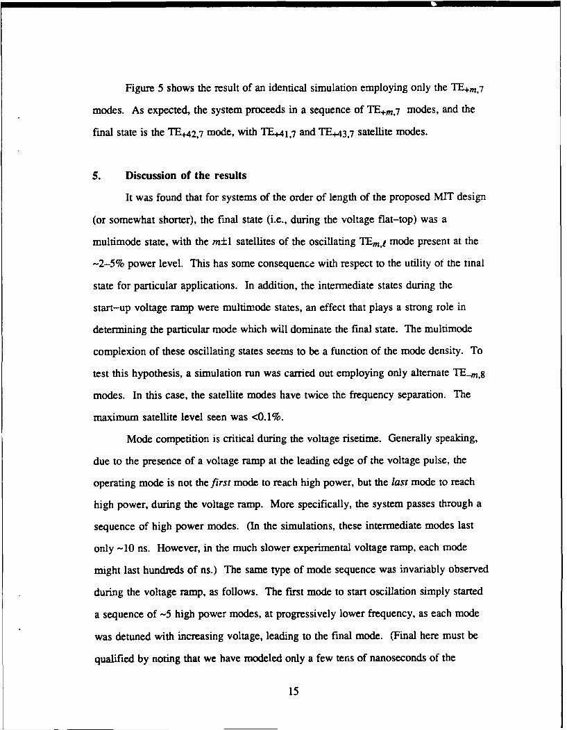
Figure 5 shows the result of an identical simulation employing only the TE+m,7

modes. As expected, the system proceeds in a sequence of TE+m,7 modes, and the

final state is the TE+42,7 mode, with TE+4 1,7 and TE+43,7 satellite modes.

5. Discussion of the results

It was found that for systems of the order of length of the proposed MIT design

(or somewhat shorter), the final state (i.e., during the voltage flat-top) was a

multimode state, with the m±1 satellites of the oscillating TEm,t mode present at the

-2-5% power level. This has some consequence with respect to the utility ot the tinal

state for particular applications. In addition, the intermediate states during the

start-up voltage ramp were multimode states, an effect that plays a strong role in

determining the particular mode which will dominate the final state. The multimode

complexion of these oscillating states seems to be a function of the mode density. To

test this hypothesis, a simulation run was carried out employing only alternate TE-m,8

modes. In this case, the satellite modes have twice the frequency separation. The

maximum satellite level seen was <0.1%.

Mode competition is critical during the voltage risetime. Generally speaking,

due to the presence of a voltage ramp at the leading edge of the voltage pulse, the

operating mode is not the first mode to reach high power, but the last mode to reach

high power, during the voltage ramp. More specifically, the system passes through a

sequence of high power modes. (In the simulations, these intermediate modes last

only -10 ns. However, in the much slower experimental voltage ramp, each mode

might last hundreds of ns.) The same type of mode sequence was invariably observed

during the voltage ramp, as follows. The first mode to start oscillation simply started

a sequence of -5 high power modes, at progressively lower frequency, as each mode

was detuned with increasing voltage, leading to the final mode. (Final here must be

qualified by noting that we have modeled only a few tens of nanoseconds of the

15

voltage flat-top, and the apparent stability during this time interval may not persist for

the microseconds of the experimental voltage pulse.) We have found that each

intermediate state ir a multimode state, since when a TEm,t mode is large, it will have

satellites at TEm,,1 ,I. This is a result of a "well-understood" process (Levush and

Antonsen 1990) whereby the TEm±l,l modes grow up due to a resonance condition

involving 2cpmt-om+I,t-om~-,1c0. However, TEm',. modes in other radial series

1W I, with m'*m±l, do not become satellites, and in fact are found in the simulations

to be strongl" suppressed. Since the satellite modes are from the same set of radialmodes (e.g., TE+m,7 o TE~m,8 modcs), the lower frequency TE±mTI,l satellite mode

will have both gain and higher initial amplitude than other competing modes, just as

the TE+m t mode detunes out of its nonlinear operation due to the effect of the positive

voltage ramp.

In fact, the simulations indicate the situation is still more strongly biased in

favor of the lower frequency satellite mode. That is, the TE-.,TI,t mode, which begins

at z 1% of the power of the main mode (or z 10% of its rf electric field), will begin to

grow and ultimately to suppress the TE+mt mode, due to the voltage ramp, so that the

TE±n,t mode actually turns off at a slightly lower voltage than it would in a single

mode run. Thus, no other modes have much likelihood of taking over, and there is a

strong tendency for the system to evolve in a .iequence of modes with constant radial

index (and constant sense of rotation), even if it would appear that at full voltage, this

set of modes does not have the lowest threshold current (highest growth rate).

There is a window in time during which the dominant mode has begun to fall off,

and the lower frequency satellite mode to grow, during which other modes can also

compete. However, it is a very limited window. That is, while the satellite is growing

by only -100x in power to saturation (and only -30x to the point at which nonlinear

suppression of other modes begins), another mode would have to come out of the

noise level (which was arbitrarily set at 1 kV/cm at the beam for each mode), and

16A-

grow large enough to suppress the satellite mode. Since this competition is based on

relative growth rates, rather than the voltage risetime, it is not necessary to simulate

a ramp as slow as the experimental ramp (several microsecond risetime) to

adequately model this aspect of mode competition.

Therefore, to design for operation in the TE+42,7 mode, for instance, it is not

sufficient to ensure that this mode has the lowest starting current in the vicinity of the

final voltage. In practice, at the beam radius chosen to optimize the coupling to the

TE+4 2,7 mode, the TE-m,8 modes always start first, and thus the final state is instead

the TE- 39 ,8, even though this mode has a higher starting current in the vicinity of the

design voltage. Instead, one must ensure that a higher frequency TE+m,7 mode, such

as the TE+4 5,7 mode, is the first mode to start oscillation during the rise of the voltage

ramp.

To test this supposition, a search was made for a beam radius at which a

TE+m,7 mode would oscillate first. Figure 6 shows the starting current as a function of

voltage for the case of B0 =1 1.265 T and rblRw=0.624, corresponding to a beam radius

of 0.780 cm. In this case, the TE+47 ,7 mode should be the first mode to oscillate,

followed by the TE+46,7 . (However, there is a small interval near 32 keV where the

TE- 4 3,8 mode has the lowest starting current.) Figure 7 shows the results of a

time-dependent simulation run for this beam radius. (The remaining parameters are

as in Fig. 2.) As expected, the TE+m,7-mode series dominates in a sequence

beginning with the TE47,7 mode and ending with the TE+42 ,7 mode. The TE-4 3,8 mode

shows some growth at -10 ns, but is quickly suppressed by the TE+46 ,7 mode. This

simulation run included the TE.-m,7 modes as well, since the TE-42,7 mode actually has

a lower starting current than the TE+4 2 ,7 mode. However, the progression is a series

of TE+m,7 modes, as predicted from the previous long simulation, and, despite its

higher linear growth rate, the TE-42,7 mode is completely suppressed in the final

state, because the TE+42,7 mode was already present at a significant level as the

17

system detuned with voltage from the TE+4 3 ,7 mode. The saturated state again

appears to be a multimode state, with substantial amounts of the TE+43, 7 and TE+4 1,7

modes present.

6. Summary

We have carried out a simulation study of mode competition in highly

overmoded gyrotron oscillators. The parameters of our simulation were chosen in light

of a 280 GHz, 1 MW gyrotron design from MIT. The study addressed the difficulty of

causing the system to oscillate in the design mode in the presence of competition from

other modes, and demonstrated the difficulty of achieving stable single-mode

operation. While the simulations were computationally intensive, and could not

pursue all issues relevant to long pulse operation, they were used to study numerous

separate cases, and established trends with respect to the problems of mode

competition during the start of the voltage pulse. They also addressed the mode

purity of the final state. Specifically, it was found that because of multimode coupling,

the system had a very strong tendency to remain in a particular series of TEmj modes,

with m of a particular sign, and I constant, during the voltage ramp. Thus, controlling

the first mode to oscillate can permit control of the final mode to oscillate, even in the

presence of substantial competition from modes with different values of 1. The

efficiency of the final state depends strongly on the final detuning (as well as on the

presence of parasitic modes). In general, the optimum detuning derived for a single

mode was unachievable due to mode competition. Finally, for systems of the length of

the MIT design (or somewhat shorter), the final state appears to be a multimode

state, with the TEml:,n modes present at approximately the 3-5% level. This will

degrade the useful efficiency of the gyrotron for many applications. In addition, the

efficiency is somewhat degraded because the magnetic field detuning that optimizes

efficiency in a single mode run, will not generally result in operating in the same mode

in the presence of mode competition.

18

ACKNOWLEDGMENTS

We acknowledge useful discussions with W.M. Manheimer. This work was

supported in part by the U. S. Office of Naval Research and in part by the Office of

Fusion Energy of the U. S. Department of Energy. The Cray computer time was

provided by an NRL 6.1 Cray X-MP Production Time Grant.

19

References

ANTONSEN, T., LEVUSH, B., and MANHEIMER, W. M., 1990, Stable single mode

operation of a quasioptical gyrotron. Physics of Fluids B, 2, 419-426.

BONDESON, A., MANHEIMER, W. M., and OTr, E., 1983, "Multimode analysis of

quasi-optical gyrotrons and gyroklystrons" in Infrared and Millimeter Waves,

edited by Button, K.J. (Orlando: Academic Press), vol. 9, chap. 7, pp. 309-339.

BORIE, E. and JODICKE, B., 1988, Comments on the linear theory of the gyrotron.

IEEE Transactions on Plasma Science, 16, 116-121.

DANLY, B. G., and TEMKIN, R. J., 1986, Generalized nonlinear harmonic gyrotron

theory. Physics of Fluids, 29, 561-567.

DUMBRAJS, 0., NUSINOVICH, G. S., and PAVELYEV, A. B., 1988, Mode competition

in a gyrotron with tapered external magnetic field. International Journal of

Electronics, 64, 137-145.

FLIFLET, A. W., READ, M. E., CHU, K. R., and SEELEY, R., 1982, A self-consistent

field theory for gyrotron oscillators: application to a low Q gyromonotron.

International Journal of Electronics, 53, 505-522.

FLIFLET, A. W., 1986, Linear and nonlinear theory of the Doppler-shifted cyclotron

resonance maser based on TE and TM waveguide modes. International

Journal of Electronics, 61, 1049-1080.

FLIFLET, A. W., LEE, R. C., GOLD, S. H., MANHEIMER, W. M., and OTr, E., 1991,

Time-dependent multimode simulation of gyrotron oscillators. Physical

Review A, in press.

GRIMM, T., 1991, private communications.

KREISCHER, K., 1991, private communications.

LAMB, W. E., JR., 1964, Theory of an optical maser. Physical Review, 134, A1429-

A1450.

20

LEVUSH, B., and ANTONSEN, T.M., JR., 1990, Mode competition and control in

high-power gyrotron oscillators. IEEE Transactions on Plasma Science, 18,

260-272.

LIN, A. T., LIN, C.-C., YANG, Z. H., CHU, K. R., FLIFLET, A. W., and GOLD, S.H.,

1988, Simulation of transient behavior in a pulse-line-driven gyrotron

oscillator. IEEE Transactions on Plasma Science, 16, 135 -141.

MOISEEV, M. A., and NUSINOVICH, G. S., 1974, Concerning the theory of multimode

oscillation in a gyromonotron. Izvestia Vysshikh Uchebnykh Zavedenni,

Radiofizika, 17, 1709 (Radiophys. Quantum Electron., 17, 1305).

NUSINOVICH, G. S., 1981, Mode interaction in gyrotrons. International Journal of

Electronics, 51, 457-474.

SARGENT, M., III, SCULLY, M. 0., and LAMB, W.E., Jr., 1974, Laser Physics

(Reading, Mass.: Addison-Wesley), chap. 8.

21

!A

100

-TE+427md

TEm,8moe

-TE~m,7moe60 1

-Other modes

Beam line

40-44,8

+47,7

20

0 . .0 10 20 30 40 50 60 70 80

V beam (keV)Figure 1. start current calculations for the MIT pyrotron design (but with L/.)-8.26),

for Bo= 11.265 T, rWIRw=O. 6.

22

m) C) -~ 64L - 6rz0 6 C

0 i m~ Itlq I* II Iq Iq Rt m m mmI I II I I I I I

0~ ~ c* Ke ts a4 aQoo

(AG ) e61211A W'e8l

C)~0 0 * >

C 0

Cf) to

(4-)

ItI

E2

co LoC)C~ D oz

c 0

o

C*1j

0

(M) JOMOd in(;+no c

23

35

30

25

-0

~20C

S15

0

00

5

00 10 20 3Q 40 50 60 70 80 90

t (nsec)Figure 3. Efficiency from the simulation.

24

10 6 90

----Beam Voltage --

80

10

70

600

7 E

o 0 +46,7 +42,7 50 M+43,7 0

+4340

0 10 20 30 40 50 60 70 80 90t (nsec)

Figure 4. Plot of only the TE+m,7 modes from the simulation.

25

.* -* -T *III It

(AOi) e6egloA We89

co 0

0 c

0 0.0)3

co

E 000k -

co 0

00C')(0

0 00 0)0i _o

E~

(+ e~ nll v

26Z

100

80 T+m,7 mode

601

20

0 10 20 30 40 50 60 70 80V beam (keV)

Figure 6. Start current calculations for B0=1 1.265 T, r/Rw,=O.624.

27

c IT It It 14t IT IT 14 It CV IV)V-n

rA

0~~~ 0

(ABA) eGMIOA UeGGC> CD 0D 0 0C0oa) C -CD Lnc'

oY Lo e00

0

c4- E

oc

0

S EC> C

00

0 0 00000

(M) JOMOd pIn Cf"

28