multimodal functional neuroimaging: new insights from ... · (franco battiato) iii acknowledgments...
TRANSCRIPT
UNIVERSITÀ DEGLI STUDI DI TRIESTE
Sede Amministrativa del Dottorato di Ricerca
XXII CICLO DEL
DOTTORATO DI RICERCA IN
INGEGNERIA DELL’INFORMAZIONE
Multimodal functional neuroimaging: new insights
from novel head modeling methodologies
Settore scientifico disciplinare: ING-INF/06 – Bioingegneria Elettronica e Informatica
DOTTORANDO: RESPONSABILE DOTTORATO DI RICERCA
Fabio MENEGHINI Chiar.mo Prof. Roberto VESCOVO
_______________________________
RELATORE
Dott. Ing. Federica VATTA (Università di Trieste)
_______________________________
CORRELATORE
Chiar.mo Prof. Francesco DI SALLE (Università di Salerno)
_______________________________
ANNO ACCADEMICO 2009-10


ii
Dentro di me vivono la mia identica vita dei microrganismi che
non sanno di appartenere al mio corpo... Io a quale corpo ap-
partengo?
(Franco Battiato)

iii
Acknowledgments
The present work, as a result of four years spent researching and investi-
gating the physical mechanisms underlying the brain phenomena, is almost
entirely based on the analysis of data acquired at the Maastricht Brain Imag-
ing Center (M-BIC), Faculty of Psycology and Neuroscience, Department of
Cognitive Neuroscience of the University of Maastricht (Maastricht, NL). This
is why my first sincerest gratitude goes to the M-BIC Directors, prof. Fran-
cesco Di Salle and prof. Rainer Goebel, and to all the scientists, research and
technical staff that introduced me in the latest cutting-edge advancements in
data acquisition and processing technologies.
“Those were the days” so the title of an old popular song reads. This is
the literal expression that usually comes in my mind whenever I recall any-
one of the single day from the last four years. Four years dense of expecta-
tions, emotions, and life. I will always be grateful to my wife for supporting me from the very first day this journey -that we call PhD -started from, especially for her lovable pa-tience during my experience at the Maastricht University, where the most significant part of my studies –and one of the most exciting parts of my life- took place. Thanks to Tommaso, Matteo e Michele, for being there sharing their thoughts, their life with mine, always making me feel at the right moment in the right place, even (and especially) when everything seemed to go wrong. Thanks al-

iv
so to Barbara, Claudia and Rosy, because in many of the funniest moments I will ever remember there are their beautiful smiles. Eventually my special thanks go to prof. Francesco Di Salle and Federica Vat-ta, who always believed in me from the very first moment, because without their wise support nothing of this would have ever happened. Last, but not least, thanks to my sons, just for coming into existence, thus making our lives brighter and worthier day by day.

v
List of contents
Acknowledgments ............................................................................... 3
List of contents .................................................................................... 5
List of abbreviations .......................................................................... 10
1 Introduction .............................................................................. 11
1.1 Motivation of the study ......................................................... 11
1.2 Overview ................................................................................ 13
2 State of the art in functional neuroimaging ................................ 15
2.1 Diffusion Weighted Imaging .................................................. 16
2.1.1 Physiological diffusion .................................................. 16
2.1.2 Diffusion Tensor Imaging ............................................. 19
2.2 EEG-based source imaging ..................................................... 22
2.2.1 Basics of neurophysiology ............................................ 23
2.2.1.1 Physiology of the neuron ......................................... 25
2.2.1.2 Generation of EEG signal ......................................... 26
2.2.1.3 Anisotropy characterization .................................... 28
2.2.2 EEG forward problem ................................................... 30
2.2.2.1 Source model ........................................................... 35
2.2.2.2 Lead Field ................................................................. 36
2.2.3 Head models and forward problem solution ............... 39
2.2.3.1 Analytical solution and spherical models ................ 40
2.2.3.2 Boundary Element Method ..................................... 43

vi
2.2.3.3 Finite Difference Method ........................................ 46
2.2.4 EEG inverse modelling .................................................. 54
2.2.4.1 Weighted Minimum Norm approach ...................... 56
2.2.4.2 Laplacian-WMN and LORETA ................................... 57
2.2.4.3 Local Autoregressive Average ................................. 58
2.2.4.4 Spatial filter normalization ...................................... 58
2.2.4.5 The regularization parameter .................................. 59
2.2.4.6 Scanning approaches: beamforming ....................... 60
2.3 fMRI source imaging .............................................................. 61
2.3.1 Neurovascular coupling and BOLD effect ..................... 61
2.3.2 Statistical analysis of functional data: GLM.................. 62
2.3.2.1 Statistical mean comparison ................................... 63
2.3.2.2 t Test ........................................................................ 63
2.3.2.3 Correlation Analysis ................................................. 64
2.3.2.4 General linear model ............................................... 65
2.4 EEG-fMRI integration ............................................................. 67
2.4.1 fMRI-constrained distributed inverse modelling ......... 68
2.4.2 fMRI-Guided Equivalent Current Dipole Fitting ........... 68
2.4.3 fMRI-Constrained Cortical Current Imaging ................. 69
2.4.4 Multimodal Beamforming ............................................ 72
2.4.5 EEG Source Analysis with EEG-fMRI Coupling .............. 72
2.4.5.1 Background .............................................................. 72
2.4.5.2 Processing ................................................................ 73
2.4.5.3 Experimental note ................................................... 74
3 Comparative analysis of different head modelling approaches in EEG-based functional
neuroimaging ......................................................................................... 75
3.1 Aim of the study ..................................................................... 75
3.2 Sensors and sources ............................................................... 76

vii
3.3 Building of the MNI-template-based realistic model ............. 76
3.3.1 Workflow overview ...................................................... 78
3.3.2 DWI Data ...................................................................... 80
3.3.3 Voxel Based Morphometry procedure ......................... 80
3.3.4 Target subject and template determination ................ 81
3.3.5 Application of Tract Based Spatial Statistics (TBSS) ..... 82
3.3.6 Eigenvectors estimation ............................................... 82
3.3.7 From conductivity tensors to diffusion tensors ........... 84
3.3.8 Skull conductivity anisotropy ....................................... 85
3.3.9 Effects of anisotropy in Lead Field computation .......... 85
3.4 Spherical modelling approach................................................ 86
3.5 BEM modelling approach ....................................................... 87
3.6 Comparison methods ............................................................. 88
3.6.1 Point Spread Function (PSF) analysis ........................... 88
3.6.2 Full width at half maximum (FWHM) parameter ......... 90
3.6.3 Mutual Correlation (MC) .............................................. 91
3.7 Comparative analysis of different modelling approaches: spherical spherical vs.
realistic geometry ..................................................................................... 91
3.7.1 PSF maps ...................................................................... 91
3.7.2 Extended FWHM values maps ...................................... 92
3.7.3 MC maps ...................................................................... 93
3.8 Evaluation of effects led by model geometrical differences .. 94
3.9 Increasing model complexity: comparative analysis of the three different modelling
approaches 98
3.9.1 PSF maps ...................................................................... 98
3.9.2 Extended FWHM values map ..................................... 101
3.10 Evaluation of the effects given by different modelling choices102

viii
4 Application to EEG-fMRI multimodal integration ...................... 107
4.1 Aim of the study ................................................................... 107
4.2 Building of the realistic model ............................................. 108
4.3 Experimental design ............................................................. 108
4.4 fMRI activation imaging ...................................................... 109
4.5 EEG distributed source analysis ........................................... 112
4.5.1 Channel pre-processing .............................................. 112
4.5.2 Covariance calculation ............................................... 113
4.5.3 Inverse Modeling ........................................................ 113
4.5.4 Source time-course reconstruction ............................ 113
4.5.5 Source imaging and statistical analysis ...................... 114
4.6 EEG-fMRI distributed Source Coupling Analysis ................... 115
4.6.1 Channel pre-processing .............................................. 116
4.6.2 Single design matrix ................................................... 116
4.7 fMRI weighting of an EEG inverse solution .......................... 116
4.8 Results .................................................................................. 117
4.8.1 EEG-source analysis .................................................... 117
4.8.2 EEG-fMRI coupling ...................................................... 118
4.8.3 fMRI weighting of EEG inverse solution ..................... 118
4.9 Evaluation of brain source reconstruction capabilities ........ 118
5 Conclusions .............................................................................. 122
6 Bibliography ............................................................................. 125
7 Figures ..................................................................................... 131
8 Tables ...................................................................................... 145

ix

x
List of abbreviations
CNS: Central Nervous System PET: Positron Emission Tomography fMRI: Functional Magnetic Resonance Imaging DWI: Diffusion Weighted Imaging DTI: Diffusion Tensor Imaging MRI: Magnetic Resonance Imaging EEG: ElectroEncephaloGraphy MEG: MagnetoEncephaloGraphy ECD: Equivalent Current Dipole DECD: Distributed Equivalent Current Dipole HCM: Head Conductor Model FDM: Finite Difference Method BEM: Boundary Elements Method FEM: Finite Element Method WMN: Weighted Minimum Norm PSF: Point Spread Function dSPM: Dynamic Statistical Parametric Maps BOLD: Blood Oxygen Level Dependent (signal) VBM: Voxel-based Morphometry TBSS: Tract based Spatial Statistics GLM: General Linear Model

1 Introduction
1.1 Motivation of the study
Localization of neural brain sources is important in several areas of re-
search of basic neuroscience, such as cortical organization and integration, and
in some areas of clinical neuroscience such as preoperative planning [1] and
epilepsy [2].
Neuroimaging techniques, aimed to the visualization of the cerebral activ-
ity, can be grouped into two main categories: those based on the variation of
hemodynamic parameters, such as blood flux, volume, oxygen and or glucose
consumption, that are implicitly related to the neural activity, and those based
on direct measurement of the neuronal bioelectricity. The former includes techniques such as Positron Emission Tomography (PET) and Functional Magnetic Resonance Imaging (fMRI) which, thanks to its non-invasiveness, it results the most widely used in neuroimaging. The fMRI exhi-bits a high spatial resolution, in the order of 2-4 mm, but temporal resolution is limited by the typical hemodynamic response timings, which are about 1-2 seconds, far from being able to track neuronal events, as they occur in few mil-liseconds. Techniques based on the direct measurements of the bioelectric activity in-clude ElectroEncephaloGraphy (EEG) and MagnetoEncephaloGraphy (MEG), followed by three dimensional source reconstruction algorithms. Although EEG and MEG can offer a very high temporal resolution on the order of fraction of milliseconds, still the spatial resolution reached by the reconstruction algo-rithms is severely limited by the intrinsic uncertainty margins. Focal sources can be affordably detected and described from EEG and MEG data by means of

1.1 - Motivation of the study
12
dipolar localization techniques, while non-linear methods for parametric mod-elling must be used to describe distributed activity. Both the approaches imply the definition of models of neuronal source, usually described as a patch of Equivalent Current Dipole (ECD), as well as the defini-tion of a volume conductor model, which can be realistic or approximated. The two kinds of approaches thus have complementary features in terms of spatio-temporal resolution, from here the idea to combine the two data analy-sis in the so-called multimodal integration. Thanks to these advanced analysis methods, it is now possible to derive 4-D cerebral maps of neural activation-deactivation patterns, that exhaustively describe cerebral activities arising from a specific task execution, starting from simple motor tasks to more com-plex cognitive and behavioural processes. In this perspective, EEG was pre-ferred instead of MEG because of the possibility to acquire EEG and fMRI data simultaneously [3]. Up to now, EEG-fMRI has been mainly seen as an fMRI technique in which the synchronously acquired EEG is used to characterize brain activity across time allowing to map, through statistical parametric map-ping for example, the associated hemodynamic changes [4]. Outside the field of epilepsy, EEG-fMRI has been used to study event-related (triggered by external stimuli) brain responses and provided important new insights into baseline brain activity in during resting wakefulness and sleep [5] Nonetheless, it must be taken into account that different cerebral regions sup-posed to run different tasks can be no longer considered as independent, but rather as a synchronized team cooperating to successfully execute each task. This leads to the importance of studying the organized behaviour among the specific cerebral regions basing on their functional connectivity. The present dissertation is aimed to introduce a novel approach to the multi-modal functional imaging of neural sources of activity, by means of integration of MRI, EEG and fMRI data analysis.
1.2 - Overview
13
1.2 Overview
The present dissertation begins with a review of the current state-of-the-
art in the major neuroimaging techniques. Particular attention has been de-
voted to EEG modelling since it represents the main player of our studies, also
because it is one of the most promising techniques in neural sources analysis. The literature regarding EEG/fMRI multimodal integration is quite extensive even if it comes as a very recent approach; a summary of the main and com-monly used algorithm is presented. Moreover a brief overview of Diffusion Weighted Imaging and Diffusion Ten-sor Imaging is also given, as their application in modelling refinement is enormously increasing the accuracy and the complexity of the models. In chapter 3 we will discuss the accomplished comparative analysis, which re-quired the introduction of some kind of measurements in order to address the target. Chapter 4 deals with a case study and the proposal of an EEG and fMRI data processing pipeline that leads to a robust and effective neural source recon-struction. The results presented in chapter 3 have been first published in [6], and
later in [7] where a further algorithm has been involved in a deeper investiga-
tion about how different numeric techniques perform in the EEG forward
problem solution. The experiments described in chapter 4 as well as the presented results sug-gest further investigations, mainly focused on the optimal tuning of the many parameters involved in the source imaging application described. However, due to their relevance, they will be soon submitted for a methodology study to Neuroimage journal.

1.2 - Overview
14
Besides, two more papers had been previously published, focusing on the im-plementation, validation [8] and application [9] of the algorithm described in section 2.2.3.3, in a High Performance Computing environment.
1.2 - Overview
15
2 State of the art in functional neuroimaging
In this section a synthetic overview of the currently most widely used
techniques in functional neuroimaging is presented. Magnetoencephalography (MEG) and Electroencephalography (EEG) provide a unique window on the human brain. Both modalities measure the electro-magnetic signals produced by electrical activity in the brain. It is widely be-lieved that the primary source of these signals is current flow in the apical dendrites of pyramidal cells in the cerebral cortex. Coherent activation of a large number of pyramidal cells small areas of cortex can be modelled as an equivalent current dipole (ECD), which, because of the columnar organization of cortex, is oriented normally to its surface. The current dipole is therefore the basic element used to represent neural activation in EEG and MEG based inverse methods, and these dipoles are often constrained to lie within cortical gray matter. Current technologies provide EEG acquisition systems fully compatible with the conventional MRI environment, i.e. high static magnetic field and strong RF electromagnetic pulses gradients. As these new features make possible the contemporary measurements of both hemodynamic response and neuronal electrical activity, we are focusing on EEG, rather than MEG signal processing to accomplish an effective multimodal integration, which will be described in the last paragraph of this chapter.

2.1 - Diffusion Weighted Imaging
16
2.1 Diffusion Weighted Imaging
Diffusion-weighted magnetic resonance imaging (MRI) is an emerging
neuroimaging technique which has been boosted by established successes in
clinical neurodiagnostics and by powerful new applications for studying the
brain in vivo.
Measurement of signal attenuation from water diffusion is one of the most
important issues for operating diagnosis in the central nervous system (CNS).
In particular, diffusion tensor imaging (DTI) may be used to map and charac-
terize the three-dimensional diffusion of water as a function of spatial location.
The diffusion tensor thus obtained describes the magnitude, the degree of ani-
sotropy, and the orientation of diffusion anisotropy.
Many developmental, aging, and pathologic processes of the CNS influence
the microstructural composition and architecture of the affected tissues. In the
above cited conditions, the diffusion of water within tissues results to be al-
tered by changes in the tissue microstructure and organization; consequently,
diffusion-weighted (DW) MRI methods, including DTI, are extremely powerful
probes for characterizing the effects of disease and aging on microstructure.
2.1.1 Physiological diffusion
Diffusion is a random transport phenomenon, which describes the transfer
of material from one spatial location to other locations over time. In three di-
mensions, the Einstein diffusion equation is:
tn
rD
∆
>∆<=2
2
where the diffusion coefficient D (in mm2/s) is proportional to the mean
squared displacement <∆r2> divided by the number of dimensions, n , and the

2.1 - Diffusion Weighted Imaging
17
diffusion time, t . The diffusion coefficient of water at 37°C is roughly 3.0x10⁻⁹
mm2/s and increases at higher temperatures. In absence of boundaries, mo-
lecular water displacement is described by a Gaussian probability density:
( )( )
∆∆−
∆=∆∆
tD
r
tDtrP
4exp
2
1,
2
3π
The spread in this distribution increases with the diffusion time, t. The diffu-sion of water in biological tissues occurs through cellular structures. Water dif-fusion is primarily caused by random thermal fluctuations. The behaviour is further modulated by the interactions with cellular membranes, and subcellu-lar and organelles. Cellular membranes hinder the diffusion of water, causing water to take more tortuous paths, thereby decreasing the mean squared dis-placement. In fibrous tissues, including white matter, water diffusion is rela-tively unimpeded in the direction parallel to the fibres orientation. Conversely, water diffusion is highly restricted and hindered in directions perpendicular to the fibres. Thus, the diffusion in fibrous tissues is anisotropic. The application of the diffusion tensor to describe anisotropic diffusion behaviour was intro-duced by Basser [10], [11]. In this model, diffusion is described by a multiva-riate normal distribution: ( )
( )
∆∆∆−
∆=∆∆
−
t
rDr
DttrP
T
4exp
2
1,
1
3
rrrr
π
where the diffusion tensor D is a 3x3 covariance matrix:
=
zzzyzx
yzyyyx
xzxyxx
DDD
DDD
DDD
D
which describes the covariance of diffusion displacements in three dimensions normalized by the diffusion time. The diagonal elements (Dii>0) are the diffu-sion variances along the axes x ,y , and z, and the off-diagonal elements are the

2.1 - Diffusion Weighted Imaging
18
covariance terms and are symmetric about the diagonal (Dij=Dji ). Diagonaliza-tion of the diffusion tensor yields the eigenvalues (λ1,λ2,λ3) and corresponding eigenvectors (eeee1,eeee2,eeee3) of the diffusion tensor, which describe the directions and apparent diffusivities along the axes of principal diffusion. Moreover, a tensor represents a physical state and it is a geometric object
that has invariant properties when the coordinate system is rotated. A scalar
for instance does not change with the rotation, a vector can be represent as an
arrow in space with direction and magnitude and even if the components
might change during rotation of coordinate system the direction and magni-
tude are invariant. As a consequence, the complete set of tensor’s element can
be computed by
F = G HIJ 0 00 IK 00 0 ILM GNJ
where S is orthogonal matrix of unit length eigenvectors of the measured
diffusion tensor. The diffusion tensor may be visualized as an ellipsoid, with the eigenvectors defining the directions of the principal axes and the ellipsoidal radii defined by the eigenvalues (Figure 2-1). Diffusion is considered isotropic when the eigen-values are nearly equal (λ1~λ2~λ3). Conversely, the diffusion tensor is aniso-tropic when the eigenvalues are significantly different in magnitude (λ1>λ2>λ3). The eigenvalue magnitudes may be affected by changes in local tissue microstructure with many types of tissue injury, disease, or normal phy-siological changes. Thus, the diffusion tensor is a sensitive probe for characte-rizing both normal and abnormal tissue microstructure.

2.1 - Diffusion Weighted Imaging
19
Figure 2-1The diffusion ellipsoids and tensors for isotropic unrestricted diffusion, isotropic restricted diffusion,
and anisotropic restricted diffusion are shown.
In the CNS, water diffusion is usually more anisotropic in white matter re-
gions and isotropic in both grey matter and cerebrospinal fluid (CSF). The ma-
jor diffusion eigenvector (e1, direction of greatest diffusivity) is assumed to be
parallel to the tract orientation in regions of homogeneous white matter. This
directional relationship is the basis for estimating the trajectories of white
matter pathways with tractography algorithms.
The diffusion tensor model performs well in regions where there is only
one fibres population (fibres are aligned along a single axis), where it gives a
good depiction of the fibres orientation. However, it fails in regions with sev-
eral fibres populations aligned along intersecting axes because it cannot be
used to map several diffusion maxima at the same time. In such areas, imaging
techniques that provide higher angular resolution are needed.
2.1.2 Diffusion Tensor Imaging
Maps of DTI measures are estimated from the raw DW images. The first
step in the calculation of the diffusivities tensor is to estimate the apparent dif-

2.1 - Diffusion Weighted Imaging
20
fusivity maps, Di,app, for each encoding direction. The following equation de-
scribes the signal attenuation for anisotropic diffusion with the diffusion ten-
sor:
( ) ( )appiii
T
ii DbSgDgbSS ,00 expˆˆexp −=−=
where Si is the DW signal, the index i corresponds to a unique encoding di-
rection, is the unit vector describing the DW encoding direction, and bi is the
amount of diffusion weighting. In the case of single diffusion weighting (b -
value) and an image with very little or no diffusion weighting (S0), the appar-
ent diffusivity maps are estimated via:
i
iappi
b
SSD
)ln()ln( 0,
−=
Subsequently, the six independent elements of the diffusion tensor (Dxx,
Dyy, Dzz, Dxy=Dyx, Dxz=Dzx , and Dyz=Dzy ) may be estimated from the apparent
diffusivities using multiple linear least squares methods [11], [12] or nonlin-
ear modelling [13].
The display, meaningful measurement, and interpretation of 3D image
data with a 3x3 diffusion matrix at each voxel is a challenging or impossible
task without simplification of the data. Consequently, it is desirable to distil the
image information into simpler scalar maps. The two most common measures
are the trace and anisotropy of the diffusion tensor. The trace of the tensor, or
sum of the diagonal elements of D, is a measure of the magnitude of diffusion
and is rotationally invariant. The MD (also called the apparent diffusion coeffi-
cient, or ADC) has been used in many published studies and is simply the trace
divided by 3 (MD=Tr/3), which is equivalent to the average of the eigenvalues.
The degree to which the diffusivities are a function of the DW encoding direc-
tion is represented by measures of diffusion anisotropy. Many measures of
anisotropy have been described, most of which are rotationally invariant. Cur-

2.1 - Diffusion Weighted Imaging
21
rently, the most widely used invariant measure of anisotropy is the fractional
anisotropy (FA) described originally by Basser and Pierpaoli [13]:
( ) ( ) ( )( )232
2
2
1
2
3
2
2
2
1
2
3
λλλλλλ
++−+−+−
=MDMDMD
FA
Note that the FA does not describe the full tensor shape or distribution.
This is because different eigenvalues combinations can generate the same val-
ues of FA [14]. Although FA is likely to be adequate for many applications and
appears to be quite sensitive to a broad spectrum of pathological conditions,
the full tensor shape cannot be simply described using a single scalar measure
[14]. The tensor shape can, however, be described completely using a combi-
nation of spherical, linear, and planar shape measures [14], [15].
In general, it is important to consider alternative quantitative methods
when trying to interpret DTI measurements. Another important measure is the
tensor orientation described by the major eigenvector direction. For diffusion
tensors with high anisotropy, the major eigenvector direction is generally as-
sumed to be parallel to the direction of white matter tract, which is often rep-
resented using a red–green–blue (RGB) color map to indicate the eigenvector
orientations [16], [17].
The local eigenvector orientations can be used to identify and parcellate
specific WM tracts; thus, DT-MRI has an excellent potential for applications
that require high anatomical specificity. The ability to identify specific white
matter tracts on the eigenvector color maps has proven useful for mapping
white matter anatomy relative to lesions for preoperative planning [18] and
postoperative follow-up [19].
Maps of the MD, FA, major eigenvector direction, and eigenvalues are
shown as examples in Figure 2-2.

2.2 - EEG-based source imaging
22
Figure 2-2 Quantitative maps from a diffusion tensor imaging (DTI) experiment
2.2 EEG-based source imaging
EEG data are measurements of potential differences on the scalp resulting
from ohmic currents induced by electrical brain activity. Instrumentation for
EEG consists of a set of scalp electrodes coupled to high-impedance amplifiers
and a digital data acquisition system. In EEG a detailed reconstruction of the electrical sources in the brain is usually performed by solving the so-called EEG inverse problem, the purpose of which is to find the locations and distributions of the neural sources responsible for the measured activity. Any possible model formulation of the inverse problem relies on an available solution for the companion forward problem. A forward model defines how the surface potentials at given positions on the scalp can be predicted by known sources inside the cranium, typically on the cortex sur-face. Running the forward problem iteratively, it is possible to solve the in-

2.2 - EEG-based source imaging
23
verse problem by searching for the particular bioelectric source that best fits the potential distribution measured at the scalp electrodes. As an alternative, distributed source localization approaches based on imaging (e.g., minimum norm) or beamformer inverse solution [20] are also able to recover extended sources of activated cortex with different spatial extent. Before getting into the details of the EEG source analysis, it’s convenient to take a brief introduction at what the neural sources actually are, as in the fol-lowing paragraph. 2.2.1 Basics of neurophysiology
The human brain is the most important organ in the central nervous sys-
tem. In the brain, different regions can be designated according to their motor
or higher cognitive function. For example, a specific region in the brain is re-
sponsible for hand movement, while another region processes the information
concerning language. The main task of the brain is the processing and commu-
nication of information. This information can be sent to or received from parts
of the human body or other designated regions of the human brain. The brain
is situated inside the skull and scalp, which act as a protective layer against
shock and impact. Moreover, it floats in the ventricular system which is
drained with the cerebro-spinal fluid (CSF). The CSF provides essential sub-
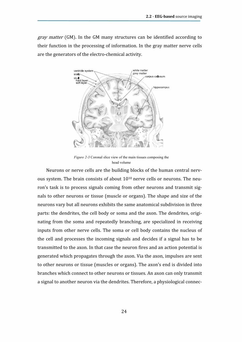
stances for the metabolism of the brain and some protection to shock. Concerning tissue types, the actual brain tissues can be divided in three parts: white matter, gray matter and the ventricles. The white matter mainly consists of connections from and to different parts of the gray matter. An important connection contained in the white matter is the corpus callosum which con-nects the right and left hemisphere. The actual brain activity is generated in the gray matter. The gray matter at the edge of the brain has a folded structure to increase the surface so complex connections can be made. The outer layer is also called the cortex or cortical
2.2 - EEG-based source imaging
24
gray matter (GM). In the GM many structures can be identified according to their function in the processing of information. In the gray matter nerve cells are the generators of the electro-chemical activity.
Neurons or nerve cells are the building blocks of the human central nerv-
ous system. The brain consists of about 1010 nerve cells or neurons. The neu-
ron’s task is to process signals coming from other neurons and transmit sig-
nals to other neurons or tissue (muscle or organs). The shape and size of the
neurons vary but all neurons exhibits the same anatomical subdivision in three
parts: the dendrites, the cell body or soma and the axon. The dendrites, origi-
nating from the soma and repeatedly branching, are specialized in receiving
inputs from other nerve cells. The soma or cell body contains the nucleus of
the cell and processes the incoming signals and decides if a signal has to be
transmitted to the axon. In that case the neuron fires and an action potential is
generated which propagates through the axon. Via the axon, impulses are sent
to other neurons or tissue (muscles or organs). The axon’s end is divided into
branches which connect to other neurons or tissues. An axon can only transmit
a signal to another neuron via the dendrites. Therefore, a physiological connec-
Figure 2-3 Coronal slice view of the main tissues composing the
head volume

2.2 - EEG-based source imaging
25
tion has to be made. This is called a synapse. The larger the dendrites, the
more connections from other neurons can be made. The synapse is a specialized interface between two nerve cells. The synapse consists of a cleft between a presynaptic and postsynaptic neuron. At the end of the branches originating from the axon, the presynaptic neuron contains small rounded swellings which contain the neurotransmitter substance. 2.2.1.1 Physiology of the neuron
At rest the intracellular environment of a neuron is negatively polarized at
approximately -70 mV compared with the extracellular environment. A neuron
can depolarize or hyperpolarize. A depolarization means that the potential dif-
ference between the intra- and extracellular environment increases. Instead of
−70mV the potential difference becomes −40mV. A hyperpolarisation means
that the potential difference between intra- and extracellular environment de-
creases. After a depolarization or hyperpolarisation occurred, the neuron returns to the resting state. This is called a repolarisation and takes some time. This is called the refractory period and the neuron cannot fire an action potential during this period. The potential difference at rest is due to an unequal distribution of Na+, K+and Cl−-ions across the cell membrane. This unequal distribution is actively maintained by the Na+and K+-ion pumps located in the cell mem-brane, providing a dynamic equilibrium. The processing and the transmission of the signals are done by an alter-
nating chain of electrical and chemical reactions. Neurons activated by an ac-
tion potential will secrete a chemical substance called a neurotransmitter, at
the synaptic side. The secretion of neurotransmitter at the presynaptic neuron
(the neuron at the axon side) is generated by action potentials. A postsynaptic
neuron (the neuron at the dendrite side) has a large number of receptors on its
membrane that are sensitive for this neurotransmitter. The neurotransmitter

2.2 - EEG-based source imaging
26
in contact with the receptors changes the permeability of the membrane for
charged ions. Two kinds of neurotransmitters exist. On the one hand there is a neurotrans-mitter which lets signals proliferate. These molecules cause an influx of posi-tive ions. Hence depolarization of the intracellular space takes place. This de-polarization is also called an excitatory postsynaptic potential (EPSP). On the other hand there are neurotransmitters that stop the proliferation of signals. These molecules will cause an outflow of positive ions. Hence a hyperpolarisation can be detected in the intracellular volume. This po-tential change is also called an inhibitory postsynaptic potential (IPSP). There are a large number of synapses from different presynaptic neurons in contact with one postsynaptic neuron. At the cell body all the EPSP and IPSP signals are integrated. When a net depolarization of the intracellular compartment at the cell body reaches a certain threshold, an action potential is generated. An action potential then propagates along the axon to other neurons. 2.2.1.2 Generation of EEG signal
The electrodes used in scalp EEG are large and are attached to the scalp, which is distant from the neurons compared to the size of the neuron. Consequently, an electrode only detects summed activities of a large number of neurons which are synchronously electrically active. The action potentials can be large in amplitude (70-110 mV) but they have a small time course (0.3 ms). A syn-chronous firing of action potentials of neighbour’s neurons is statistically un-likely. The postsynaptic potentials are the generators of the extracellular po-tential field which can be recorded with an EEG. Their time course is larger (10-20 ms). This enables the detection and measurements of summed activity of neighbour’s neurons, but their amplitude is smaller (0.1-10 mV). Apart from having more or less synchronous activity, the neurons need to be regularly arranged to result in a measurable scalp EEG signal. The spatial properties of the neurons must be so that they amplify each other’s extracellu-

2.2 - EEG-based source imaging
27
lar potential fields. Pyramidal neuron cells are a special type of neuron which consists of a large dendrite branch (so-called apical dendrite) which is oriented orthogonally to the surface of the gray matter. Neighbouring pyra-midal cells are organized so that the axes of their dendrite tree are parallel with each other and normal to the cortical surface. Hence, these cells are sug-gested to be the main generators of the EEG. The following is focused on excitatory synapses and EPSP, located at the
apical dendrites of a pyramidal cell. An analogue reasoning can be made for
IPSPs. As mentioned before, at the resting state there is a potential difference
between the inside and outside of the cell. The incoming action potential re-
leases the neurotransmitters in the cleft, which cause an influx of positive ions
at the post synaptic membrane and depolarize the local cell membrane. Positive ions will enter the cell. This causes a lack of extracellular positive ions at the apical dendrites of the post synaptic neuron. A redistribution of positive-ly charged ions also takes place at the intracellular side. These ions flow from the apical dendrite to the cell body and depolarize the membrane potentials at the cell body. Subsequently positively charged ions become available at the extracellular side at the cell body and basal dendrites. The neuron is thus an element that withdraws current from the extracellular space (a so-called current sink) and that injects a current with the same inten-sity (current source). The electrical activity can be modelled as a current di-pole. The current flow causes an electric field and also a potential field inside the human head, which extends to the scalp. One neuron generates a small amount of electrical activity in the order of fem-to-Ampere. This small amount cannot be picked up by surface electrodes, as it is overwhelmed by other electrical activity from neighbouring neuron groups. When a large group of neurons (approximately 1000) is simultaneously active, the electrical activity is large enough to be picked up by the electrodes at the surface, thus generating a meaningful EEG signal.

2.2 - EEG-based source imaging
28
Moreover, in order to produce a detectable signal the dipoles corresponding to each of the neurons should be oriented in the same direction. The superposi-tion of all these dipoles creates a sufficiently strong potential field that is sensed by the surface electrodes. A large group of electrically active pyramidal cells in a small patch of cortex can be represented as one equivalent dipole on macroscopic level [21]. It is very difficult to estimate the extent of the active area of the cortex as the potential distribution on the scalp is almost identical to that of an equivalent dipole [22]. 2.2.1.3 Anisotropy characterization
Electrical conductivity is the ability of a material to conduct electric cur-
rent. Tissues can have either isotropic or anisotropic conductivity. Anisotropy is the property for which a physical characteristic varies along dif-ferent directions, thus in an anisotropic material the value of physical mea-surement made in one direction generally differs from measurement done in other directions. The human head is composed of several layers each with different conductivity properties. Typical layers that are considered for modelling purpose are the scalp, the skull, the cerebrospinal fluid, the gray and the white matter. Several studies have been carried out about the direction-dependent conduc-tivity of some areas within the human head. Tissues such as skeletal muscles or white matter have been verified to have extremely anisotropic structure which can involve highly anisotropic conductivity values. The anisotropy of some layer was proved to be able to influence the EEG forward problem solu-tion [23], [24], [25]. Therefore for an accurate formulation of the problem it should not be neglected. Tissues significantly interested by anisotropy are the skull and the white
matter. The skull is a bony structure which provides a general framework for
the head. It protects the brain from injury and supports the structures of the
face. Human skull is normally made up of 28 bones, all of which, except for the

2.2 - EEG-based source imaging
29
mandible are joined together by sutures, rigid articulations permitting very lit-
tle movement. The human skull can be modelled as a three layered structure
consisting of a soft bone layer spongiosa, enclosed by two hard bone layers
compacta. The compact bone is characterized by a lower conductivity than the spongy
bone, this causing a direction-dependent conductivity with anisotropy ratio commonly estimated 1:10, (radial/tangential) to the skull surface [26], see Figure 2-4 where σr and σt represent the radial (longitudinal) and tangential (transversal) conductivity respectively. The white matter is one of the main solid components of the central nerv-
ous system. It forms the bulk of the deep parts of the brain and the superficial
parts of the spinal cord. Aggregates of grey matter are spread within the cere-
bral white matter. White matter is composed of axons, grouped in bundles. Axons connect vari-ous grey matter areas of the brain to each other and carry nerve impulses be-tween neurons. Nicholson made one of the early in vitro measurements prov-ing that the white matter of a cat has bigger conductivity parallel to the fibres than normal to the fibres. In this measurement the conductivity along nerve bundle resulted to be about 9 times larger than perpendicular to it [27] A more detailed and accurate measure of anisotropy has been achieved by means of diffusion weighted imaging (DWI) and diffusion tensor image (DTI) from magnetic resonance imaging (MRI).
Figure 2-4 Schematic representation of the layer structure of the skull
bones

2.2 - EEG-based source imaging
30
In their random diffusion displacements, molecules probe the structure of a tissue at a microscopic level. Molecules of water have been largely used for the investigation. During the diffusion they cross, bounce and interact with other molecules. The effect detected by a diffusion MRI provides unique information about the structure and the geometric organization of tissues. Since the diffusion is a three dimensional process and the mobility in tissues may not be the same in all direction a DTI supplies a powerful tool for anisotropy estimation [28]. The conductivity tensor can be derived directly from the water diffusion ten-sor under the assumption that they share the same eigenvectors as members of the general transport tensor [10]. Lately, a strong effort to the white matter fibre’s anisotropy analysis came
from the usage of cutting edge methodologies such as Q-ball imaging [29] and
High Angular Resolution Diffusion Imaging (HARDI), which takes advantage
from high angular DWI acquisition to sensibly improve the accuracy in anisot-
ropy description. As a result, this technique leads to diffusion representation
by means of several tensors per voxel, thus allowing detecting fibre crossing
and fibre kissing; an interesting application of this whole methodology has
been recently studied in [30].
2.2.2 EEG forward problem
A forward model implies considering one or more current dipole inside
the head and computing the electrical potentials generated at the electrode
sites on the scalp surface. The relationship between the electric potentials, at
any position, and a generic current density distribution in a linear, time-
invariant conducting volume is described by Poisson’s equation.
To derive its formulation, let us start from considering the electromagnetic fields in media or in vacuum, described by the Maxwell equations:

2.2 - EEG-based source imaging
31
W ∙ YZ[ = \]^ ( 2 . 1 )
W × Z[ − a^]^ bYZ[bc = a^ d[ ( 2 . 2 )
W × YZ[ + b Z[bc = 0 ( 2 . 3 )
W ∙ Z[ = 0 ( 2 . 4 )
where E and B are the electric and magnetic field, respectively. ]^ and a^ are the permeability and susceptibility of vacuum, respectively, which can be re-late to the speed of light e = 1/f(a^]^), ρ is the charge density, which is the amount of charge in a volume G (unit C/m3). As shown in the previous section the generators of the EEG can be described by a current source and sink or a current dipole source. A current corresponds to charges in motion and can be described by a current density, which is the current passing through an elementary surface. The current density J(x, y, z) is a 3D position-dependent vector field, where the direction of the vector indi-cates the direction of motion of the charges. The unit of the current density is A/m2. The divergence of a vector field J is defined as follows:
W ∙ d[ = ijkl→^1n o d[ ∙ pGql ( 2 . 5 )
The integral over a closed surface ∂G represents a flux or a current through the volume G. This integral is positive when a net current leaves the volume G and is negative when a net current enters the volume G. The vector dSSSS for a surface element of ∂G with area dS and outward normal eeeen, can also be written as

2.2 - EEG-based source imaging
32
eeeen.*dSSSS. The unit of ∇·JJJJ is A/m3 and is often called the current source density, symbolized with Im. From the Maxwell equations the continuity equation can be derived: b\bc + W ∙ d[ = 0 ( 2 . 6 )
Where ρ is the charge density and ∇ JJJJ is the current source density. Equation 2.8 states that the change in charge inside a volume conductor with time must correspond to a flow of charge out through the surface of the volume conduc-tor. In other words, a current leaving or entering the volume conductor G causes a change in the total amount of charges in G. It is shown in [31] that no charge can be piled up in the conducting ex-
tracellular volume for the frequency range of the signals measured in the EEG.
At one moment in time all the fields are triggered by the active electric source.
Hence, no time delay effects are introduced. All fields and currents behave as if
they were stationary at each instance in time. These conditions are also called
quasi-static conditions. They are not static because the neural activity changes
with time, but the changes are slow compared to the propagation effects.
Therefore the charge density in the volume G is constant, thus equation ( 2 . 6 )
yields:
W ∙ d[ = 0 ( 2 . 7 )
Due to the linearity of the Maxwell equations the current density inside the vo-lume conductor, representing the human head, consists of the current density imposed by the dipole source or primary current density Jp and the current density flowing in the volume conductor or return current density Jr: d[ = d[v + d[w ( 2 . 8 )

2.2 - EEG-based source imaging
33
The return current density generates an electric field. The relationship be-tween the return current density Jr in A/m2 and the electric field E in V/m is given by Ohm’s law: d[w = xyYZ[ ( 2 . 9 )
With Σ being the position-dependent conductivity. The conductivity Σ depends entirely on the nature of the material of which the conductor is composed, the state of aggregation of its parts and its temperature. In the case of isotropic conductivities the conductivity is position-dependent scalar, σ(x, y, z). For ani-sotropic conductivities the conductivity can be written as a position depen-dent, symmetric, positive-definite second order tensor Σ, whose matrix repre-sentation Σ(x, y, z) ∈ R3×3 according to a basis (ex,ey,ez) given by: xy ≜ H|}} |}~ |}�|}~ |~~ |~�|}� |~� |�� M
and with units A/(V m) = S/m. There are tissues in the human head that have an anisotropic conductivity. This means that the conductivity is not equal in every direction and that the electric field can induce a current density compo-nent perpendicular to it. Combining equation 2.11 with equation 2.10 yields: d[ = d[v + xyYZ[ ( 2 . 1 0 )
The scalar potential field V, having volt as unit, is now introduced. This is poss-ible due to Faraday’s law (see equation 2.5) in which the time derivative of B is zero under quasi-static conditions (∇×E = 0). The link between the potential field and the electric field is given utilizing the gradient operator: YZ[ = −W� ( 2 . 1 1 )

2.2 - EEG-based source imaging
34
The vector ∇V at a point gives the direction in which the scalar field V, having volt as its unit, most rapidly increases. The minus sign in the latter equation indicates that the electric field is oriented from an area with a high potential to an area with a low potential. When equations ( 2 . 1 0 ( 2 . 1 1 ) and ( 2 . 7 ) are combined, Poisson’s differential equation is obtained in general form: W ∙ �xyW�� = W ∙ dvZZZ[ ( 2 . 1 2 )
At the interface between two compartments, two boundary conditions are im-posed. Figure 2-5 illustrates such an interface. A first condition is based on the inability to pile up charge at the interface. All charge leaving one compartment through the interface must enter the other compartment. In other words, all current (charge per second) leaving a compartment with conductivity Σ1 through the interface enters the neighbouring compartment with conductivity Σ2.
d[J ∙ ��� = d[K ∙ ��� �xyJ ∙ W�J� ∙ ��� = �xyK ∙ W�K� ∙ ���
where eeeen is the normal component on the interface.
Figure 2-5 Boundary interface between two media

2.2 - EEG-based source imaging
35
Since no current can be injected into the air outside the human head, due to the very low conductivity of the air, the Neumann boundary condition at the surface of the head reads: d[J ∙ ��� = 0
�xyJ ∙ W�J� ∙ ��� = 0 The second boundary condition only holds for interfaces between non-air compartments, it is called Dirichlet boundary condition, and states the poten-tial continuity across the interface:
�J = �K Because EEG signals are produced by ohmic current flow in the head, they are highly sensitive to the conductivity of the brain, skull, and extra cranial tissue. Consequently, solving a forward problem requires accurate knowledge of these properties. This leads to the modelling issue, i.e. the mathematical repre-sentation of actors involved in the so called forward problem, which will be discussed in the following paragraphs.
2.2.2.1 Source model
Current source and current sink inject and remove the same amount of
current I and they represent an active pyramidal cell at microscopic level.
They can be modelled as a current dipole. The position parameter rd of the di-
pole is typically chosen half way between the two monopoles. The dipole moment mmmm is defined by a unit vector eeeem (which is directed from the current sink to the current source) and a magnitude given by m =I p, with p the distance between the two monopoles. Now, considering a dipole model source into a conductor volume, we can infer a numerical representation of the dipole itself by applying the divergence op-

2.2 - EEG-based source imaging
36
erator to small volumes which will be lately be referred to as discretization vo-lumes. For any volume enclosing both dipoles sink and source, clearly the net current flux is zero, i.e. W ∙ d[v = 0
Whenever the volume encloses either the sink or the source of the dipole lo-cated at rrrrs, the integral defining the divergence operator assumes the finite value ±I (the sign depends whether sink (-) or source (+) is enclosed in the volume). As the discretization volume G approaches zero, the singularity can be written by means of the Dirac’s delta function. The superimposition of these three cases yields: W ∙ d[v = � �(� − �������) − � �(� − �����)
The Poisson’s equation hence becomes:
W ∙ �xyW�� = � �(� − �������) − � �(� − �����) (2.13)
From now on we will refer to the term source space as the union of all the possible locations for the source dipoles inside a head model. For what has been said in the paragraph 2.2.1.2, this space is usually considered coincident with the white-matter/grey-matter interface surface. 2.2.2.2 Lead Field
From the linearity of the Poisson’s equation ( 2 . 1 2 ), it follows that the
mapping from electric sources within the cranium to scalp recordings on the
outside of the scalp can be represented by a linear operator L. In fact, due to a
dipole at a position rd and dipole moment m=mx,ex+my,ey+mz,ez a potential V at
an arbitrary scalp measurement point r can be decomposed in:

2.2 - EEG-based source imaging
37
�(�, �� , �) = k}�(�, �� , �}) + k~���, �� , �~�+ k��(�, �� , ��) (2.14)
where rrrr and rrrrd are the locations of the measurement electrode and the dipole source respectively. Hence, if we consider a set of M electrodes, placed on a regular basis on the scalp surface, and one dipolar source then the latter equa-tion can be written as: ��(c) = H �J(c)⋮��(c)M = � �(�J, �� , �}) ���J, �� , �~� �(�J, �� , ��)⋮ ⋮ ⋮�(��, �� , �}) �(��, �� , �}) �(��, �� , �})� �k}(c)k~(c)k�(c)� =
�(��) ∙ �(t) (2.15) L L L L is the so-called lead-field matrix and contains information about the geome-try and conductivity of the model. Each element Li,j of the matrix LLLL(rrrrdddd) represents the electric potential one would measure at the i-th (i=1…M) electrode caused by a single unary current dipole placed in rrrrdddd and oriented along j-th axis (j=x, y, or z). In general, given a arbitrary configuration of sources, mmmm, the measured poten-tials VVVVm , and the noise in the system, nnnn, we extend equation (2.15) to the case of a distribution of N dipoles in a source space is the following:
��(c) = H �J(c)⋮��(c)M = � ∙ ��J (c)⋮�� (c)� + H �J(c)⋮��(c)M= � ∙ �(c) + �(c) (2.16)
where the columns of the matrix L ∈ lRM×3N contain the lead fields of the dipo-
lar sources for the given M-channel EEG configuration, while mi(t)=[mx(t),

2.2 - EEG-based source imaging
38
my(t), mz(t)]T represents the source activity of the current dipole placed in the
i-th node of the source space.
Since the solution to the inverse problem consists of finding m, this im-
plies two steps: building the lead field matrix L, and ‘‘inverting’’ it, once the
scalp potentials are known, and the noise is somehow guessed.
Finding the inverse of L is an ill-posed problem and its solution requires regu-
larization. There exist many different regularization methods, as well as many
papers describing their application to EEG/MEG, these will be shown in sec-
tion 2.2.4 below. All of them assume that L either is known a priori or can be
easily constructed. While it is true that L is easy to construct for simple and
approximated geometries, building the L matrix is much more complicated for
geometries based on real patient data.
In a number of application papers, researchers have been able to compute
the L basis by exploiting analytic equations for each entry in L. The equations
for the matrix entries, or kernels, for each method can be found in [32] For
most of them, the L matrix is constructed one element at a time by evaluating
the analytic expression for the potential at each recordings site the due to a
source at each location in the domain. The reciprocity theorem, validated in [33], [34], states that the potential dif-ference between two electrodes A and B, due to a dipole mmmm located at position rrrr, is proportional to the electric field in r r r r due to the activity of two current mo-nopoles, located at the very same position of the two electrodes, scaled by the current injected IAB: � ¡(�, �) = �¢ ∙ W£(�)� ¡ (2.17)
Thus the number of forward computation is limited by the number of sensors applied. Moreover, since equation (2.17) implies the computation of a gradient, it requires potential values at each node inside the conductor volume. This is

2.2 - EEG-based source imaging
39
why reciprocity fits the features of numerical volumetric algorithm for the forward problem, described in the next section. 2.2.3 Head models and forward problem solution
Solutions to Poisson’s equation are different, and are strictly related to the
characteristics of the spatial domain in which solutions are searched.
Depending on the geometry assumed for the volume conductor model, the ap-
proaches that lead to a solution for the forward problem are either numerical
or analytical. As an example, the simplest solution is the one related to a ho-
mogeneous conductor volume G with indefinite dimensions:
�(�) = 14¤| ∙ ¥ d[(��) ∙ (� − ��)|� − ��|§ p�l When a spherical geometry is assumed for the considered model, a closed-form analytical solution of the forward problem can be used [35]. For many years, this type of solution is usually adopted for MEG and EEG for-ward problems. Although spherical models provide good approximations for MEG forward solutions [36], this is typically not the case for EEG. Several approximated-geometry models have been implemented and studied over the past years [35], [37], [38], [39], [40]. Of course, they seriously lack in geometrical adherence of the assumed shape with respect to a real human head. The “sensor-fitted sphere” approach introduced in [38] fits a multilayer sphere individually to each sensor and has shown to produce some improvement over standard spherical models [41].
More accurate forward solutions become possible by using numerical al-
gorithms, such as the boundary element method (BEM) [42], finite-element
method (FEM) [43] and finite difference method (FDM) [33] algorithms. These
numerical models allow incorporating the realistic geometry of the head and

2.2 - EEG-based source imaging
40
brain after reconstruction of the anatomical structure from individual or stan-
dardized magnetic resonance imaging (MRI) data sets. Previous studies [44]
have found that a more realistic head model performs better than a less com-
plex, for example, spherical, head model in EEG simulations, since volume cur-
rents are more precisely taken into account. More specifically, the BEM ap-
proach is able to improve the source reconstruction in comparison with
spherical models, particularly in basal brain areas, including the temporal lobe
[45], because it gathers a more realistic shape of brain compartments of iso-
tropic and homogeneous conductivities by using closed triangle meshes. The
FDM and the FEM allow better accuracy than the BEM because they allow a
better representation of the cortical structures, such as sulci and gyri in the
brain, in a three-dimensional head model [46]. The effect of head model geometry on the EEG forward solution has been con-sidered in several previous studies [44]. These studies analyzed the differenc-es in EEG forward and inverse problem solution due to different spherical or realistic model geometry [36], [47], evaluated the effects of variations in the skull thickness [48] or due to different model complexity [46], presenting re-sults for particular cases of head models. 2.2.3.1 Analytical solution and spherical models
The simplest EEG head model consists of a single-layer spherical shell of
uniform conductivity σ. A closed-form solution for calculating the potential on
the outermost surface is described by [49]. In practice, a singlelayer sphere
proves too simplistic for the human head, which consists of multiple layers of
conductivity varying by as much as two orders of magnitude between the skull
and brain.
To account for the varying conductivity of brain, skull, scalp and optionally
cerebrospinal fluid, three and four multilayer concentric-sphere analytic solu-
tions have been derived, and are commonly used. These can be computed nu-
merically using a truncated Legendre series [50]. Because of their simplicity,

2.2 - EEG-based source imaging
41
reasonable computation requirements and relatively good accuracy, multi-
layer spherical models are by far the most widely used.
Methods to improve the computational efficiency of multilayer spherical
models have focused primarily on approximating the infinite Legendre series.
Following [32], a convenient formulation of the EEG/MEG forward model en-
tails with factorizing the electric field potential or the magnetic field observed
at one extra-cranial point as the product of a “field kernel” and the dipole mo-
ment of the intra-cranial source m. For electrical potentials V, the field kernel
is a 3x1 vector (k):
�(�) = �¢(�, ��) ∙ � (2.18)
Assuming that each spherical layer has uniform and constant conductivity,
rapidly computable analytic solutions exist for both EEG and MEG forward
problem. A practical formulation of the EEG kernels has been presented by
Mosher et al. (1999), that only requires vectors expressed in their Cartesian
form.
Ary et. al. in [51] recognized that a single-sphere model could, under cer-
tain circumstances, approximate a three-shell model with good accuracy. If we
let V1(r; rm, m) and V3(r; rm, m) represent the potentials function on a single-
layer and a three-layer spheres respectively, then we can approximate V3(r; rm,
m) by adjusting the location of the dipole along its radial direction rm/|rm| by a
scale factor of μ, compute the much simpler single-sphere solution and then
scale the solution by λ.
Further refinements of this general approximation concept [52], [35] re-
sulted in the remarkably accurate approximation and a convenient method for
approximating an EEG field kernel from a multi-layer spherical model as the
weighted sum of three kernels from a single-layer spherical model applied to a
modified source configurations:

2.2 - EEG-based source imaging
42
�(�, ��) = IJ ∙ �ªª(�, aJ��) + IK ∙ �ªª(�, aK��) + IL∙ �ªª(�, aL��) where:
���(�, ��) = �eJ − eK ∙ (� ∙ ��)� ∙ �� + eK ∙ «�K ∙ � eJ ∶= 14¤|«�K ∙ 2 � ∙ ��pL + 1p − 1«®
eK ∶= 14¤|«�K ∙ ¯ 2pL + p + «« ∙ p ∙ �« ∙ p + «K − (�� ∙ �)�° � ≝ � − ��
(2.19)
Zhang refers to the parameters μj and λj as the Berg eccentricity and magni-tude parameters respectively, and hence we will refer to this approach as the Berg approximation. As for the Legendre series being approximated, the pa-rameters μj and λj are dependent only on the sphere radii/conductivity profile and independent of dipole position rrrrm. In order to reduce errors introduced by the spherical approximation,
Huang et. al. [38] found the optimally fit sphere at each sensor that best ap-
proximates the true lead-field for the actual head volume. A schematic diagram of the sensor-fitted sphere model described in [38] is shown in the figure below:

2.2 - EEG-based source imaging
43
In [38], rather than find a single locally best fitting sphere for all sensors based on the head geometry, has been carried out a fitting of the spherical model on a sensor-by-sensor basis using a set of grid points within the brain. It has been shown that the optimal fitting of each sensor-related sphere can be found ei-ther minimizing the correlation with a pre-computed golden standard lead-field, .e.g. using BEM algorithm, or on a geometric basis, e.g. minimizing the distance between each sphere’s surface and all the others sensors. 2.2.3.2 Boundary Element Method
The BEM allows one to calculate the electrical potential V of a current
source in an inhomogeneous conductor by solving the following integral equa-
tion if the conducting object is divided by closed surfaces Si (i = 1, . . ., ns) into
ns compartments, each having a different enclosed isotropic conductivity |´ � .
The electrical potential at position rrrr ∈ Sk is then given by [53]:
Figure 2-6 Spherical head models. right: sensor-fitted model, executed fitting one spherical model for each
sensor. left: classic spherical model
2.2 - EEG-based source imaging
44
|µ¶�(�) = |^� (�) + 14¤ · ∆|´ ¹ �(�º)�»(�′) ∙ �º − �|�º − �|L p½′´¾¿
�À´ÁJ (2.20)
with V0 representing the potential of the source in an unlimited homogeneous medium with conductivity |^, the mean conductivity |µ¶ ≝ (|¶� + |¶ÂÃÄ)/2, and the conductivity differences ∆σÅ ≝ �|´ � + |ÂÃÄ�. To calculate the electrical fields it is necessary to approximate numerically the integrals over the closed surfaces Si of the conductor boundaries consisting of differential surface elements dS’i and with surface normal orientations �» at positions r’r’r’r’. The surfaces are described by a large number of small triangles and the inte-grals are replaced by summations over these triangle areas. Different assump-tions about the variation of the potential over the triangle area can be applied [54], [55], [56], [42], [57]: averaged, regionally constant, linear, and quadratic dependencies. The potential values or the coefficients of the basis functions used to approximate the potentials on the surface elements form a vector of unknowns, which can be solved through the following matrix formulation: ÆÇ� = ÆÈ�È + ÉÇ� Ê � = (ÆÇ − ÉÇ)NËÆÈ�È (2.21)
If one explicitly solves equation (2.21) just for the fixed number of sensor posi-tions, a transfer matrix T is obtained that relates the sensor signals to the ho-mogeneous potentials, that depends on the geometry of the surfaces and the conductivities of each region. The potential vector VVVV, containing the field dis-tribution at all skin nodes, generated by a (dipolar) source inside the inner-most compartment –the brain-, can thus be easily computed by a simple ma-trix-vector multiplication: ÌÇ = (ÆÇ − ÉÇ)NËÆÈ Ê � = ÌÇ�È (2.22)

2.2 - EEG-based source imaging
45
The column vector V0 contains the electrical potential values V0i of all BEM model nodes i at position rrrri for the source in an infinite homogeneous conduc-tor with conductivity σ^ (dipole at position rrrrj, with current density J[[): � ´ = 14¤|^ Í[ ∙ �´ − �ÎÏ�´ − �Îϧ (2.23)
To achieve a better computational performance, the LF of dipoles at positions on regular grids inside the innermost compartment were computed and stored for all virtual electrode positions on the skin mesh The LF of a dipolar source at an arbitrary position inside the volume conductor can then be approximated by three-dimensional linear interpolation between the precomputed LF of the eight closest regular grid positions [41], [58]. Finally, the potential distribution at the real electrode positions is calculated by two-dimensional linear interpolation from the three closest virtual elec-trodes [59]. Since an exact solution of the integral in eq. (2.20) is generally not achievable, an approximated solution VÐÅ(�) on surface Si may be defined as a linear combi-nation of Ni simple basis functions: �Ð�(�) = · ÑζℎÎ(�)�¿
ÎÁJ (2.24)
Where Ni is the number of discretization elements –triangles- in the i-th
interface between the volume compartments. The basis function hj(r) can be
defined in several ways. The “constant potential” formulation, for instance,
uses basis function defined as: ℎÎ(�) = Ó1 � ∈ ∆Î0 � ∉ ∆Î Õ (2.25)
2.2 - EEG-based source imaging
46
where Δ× denotes the ith planar triangle on the tessellated surface. The colloca-tion points are typically the centroids of the surface or the vertices. The coefficients Ñζ represent unknowns on surface Si whose values are de-termined by constraining ØÐÙ(Ú) to satisfy (2.20) at discrete points, also known as collocation points.
2.2.3.3 Finite Difference Method
Finite Difference Method (FDM), Finite Element Method (FEM) and
Boundary Element Method (BEM) have been largely used in many engineering
application for numerical approximation to partial differential equation solu-
tion. Analytical solutions are continuous in space and time and provide exact results for specific boundary and initial conditions. An analytical solution can be found only for a limited set of boundary conditions and initial conditions. Numerical solutions are discrete in space and time; the spatial domain is
divided into discrete elements, called the mesh or grid spacing. An approxima-
tion to the exact results is given by an estimation of the value of the derivatives
using information about the function at the discrete grid points.
Although BEM has advantages with respect to the computational complex-
ity, it is not able to handle anisotropic conductivities.
FEM and FDM are both suitable method for the present work. FDM im-
poses regular grid over the domain, whereas FEM allows arbitrary shaped
elements over the mesh. The computational work required to obtain the same
level of error by FEM and FDM varies, depending on problems and the
schemes employed however generally FDM takes less computational time and
storage space for the same number of grid points.
Given u(x) a finite and continuous function of x, because of Taylor’s theo-
rem:

2.2 - EEG-based source imaging
47
Û(Ü + ℎ) = Û(Ü) + ℎ bÛ(Ü)bÜ + 12! ℎK bKÛ(Ü)bÜK + 13! ℎL bLÛ(Ü)bÜL+ ⋯
Û(Ü − ℎ) = Û(Ü) − ℎ bÛ(Ü)bÜ + 12! ℎK bKÛ(Ü)bÜK − 13! ℎL bLÛ(Ü)bÜL+ ⋯
(2.26)
Addition of the latter two equations gives: Û(Ü + ℎ) + Û(Ü − ℎ) = 2Û(Ü) + ℎK bKÛ(Ü)bÜK + ß(ℎà) (2.27)
where ß(ℎà) represents terms containing fourth or higher powers of h. As-suming ß(ℎà) negligible compared with lower power of h yields: bKÛ(Ü)bÜK ≅ 1ℎK [Û(Ü + ℎ) − 2Û(Ü) + Û(Ü − ℎ)] (2.28)
with a leading error of order ℎK. Equation (2.28) is a central difference formula and it approximates the tangent at P by the slope of the chord AB, in the figure below.

2.2 - EEG-based source imaging
48
Moreover the slope of the tangent at P can also be approximated either by the slope of the chord PB, which gives the forward difference formula: bÛ(Ü)bÜ ≅ 1ℎ [Û(Ü + ℎ) − Û(Ü)] (2.29)
or the slope of the chord AP, which gives the backward difference formula: bÛ(Ü)bÜ ≅ 1ℎ [Û(Ü) − Û(Ü − ℎ)] (2.30)
In both cases the leading errors are O(h2). Since the numerical domain of this method is a regular 3D voxel grid, it is ne-cessary to specify the relationship between nodes and voxels. The FD formulation proposed and validated in [60] for inhomogeneous
anisotropic field problems is first derived in the two dimensional (2-D) space
for an easy understanding. The FD formulation has similarities to the one pro-
posed and implemented by Saleheen and Kwong in [61] to determine the po-
tential distribution in a canine torso during electrical defibrillation. The
method presented in [61] differs from standard FD formulations since voxels
are mapped as mesh elements and nodes of the mesh correspond to voxels’
vertexes. In the method proposed in [60], the way the mesh is developed is dif-
Figure 2-7example of finite difference approximation in 1-D: first order central, forward
and backward difference around point P
2.2 - EEG-based source imaging
49
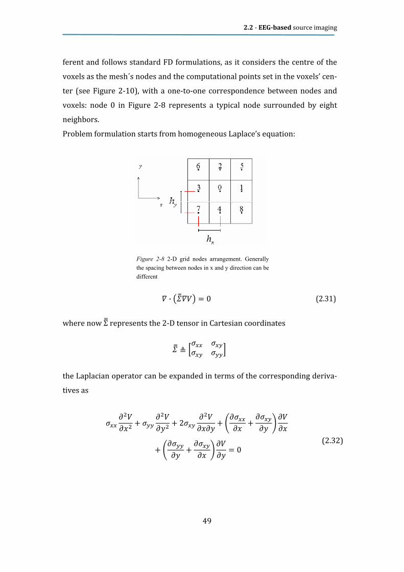
ferent and follows standard FD formulations, as it considers the centre of the
voxels as the mesh´s nodes and the computational points set in the voxels’ cen-
ter (see Figure 2-10), with a one-to-one correspondence between nodes and
voxels: node 0 in Figure 2-8 represents a typical node surrounded by eight
neighbors. Problem formulation starts from homogeneous Laplace’s equation:
W ∙ �xyW�� = 0 (2.31)
where now Σy represents the 2-D tensor in Cartesian coordinates xy ≜ â|}} |}~|}~ |~~ã
the Laplacian operator can be expanded in terms of the corresponding deriva-tives as |}} bK�bÜK + |~~ bK�bäK + 2|}~ bK�bÜbä + ¯b|}}bÜ + b|}~bä ° b�bÜ
+ ¯b|~~bä + b|}~bÜ ° b�bä = 0 (2.32)
Figure 2-8 2-D grid nodes arrangement. Generally
the spacing between nodes in x and y direction can be
different
2.2 - EEG-based source imaging
50
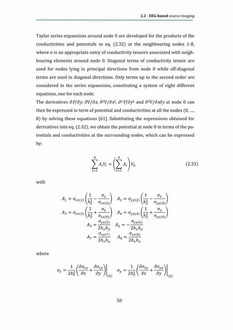
Taylor series expansions around node 0 are developed for the products of the conductivities and potentials in eq. (2.32) at the neighbouring nodes 1-8, where σ is an appropriate entry of conductivity tensors associated with neigh-bouring elements around node 0. Diagonal terms of conductivity tensor are used for nodes lying in principal directions from node 0 while off-diagonal terms are used in diagonal directions. Only terms up to the second order are considered in the series expansions, constituting a system of eight different equations, one for each node. The derivatives ∂V/∂y, ∂V/∂x, ∂2V/∂x2, ∂2V/∂y2 and ∂2V/∂x∂y at node 0 can then be expressed in term of potential and conductivities at all the nodes (0, …, 8) by solving these equations [61]. Substituting the expressions obtained for derivatives into eq. (2.32), we obtain the potential at node 0 in terms of the po-tentials and conductivities at the surrounding nodes, which can be expressed by:
with åJ = |}}(J) ¯ 1ℎ}K − |}|}}(^)° åK = |~~(K) ¯ 1ℎ~K − |~|~~(^)°åL = |}}(L) ¯ 1ℎ}K + |}|}}(^)° åà = |~~(à) ¯ 1ℎ~K + |~|~~(^)°
åæ = |~~(æ)2ℎ}ℎ~ åç = − |}~(ç)2ℎ}ℎ~åè = |}~(è)2ℎ}ℎ~ åé = |}~(é)2ℎ}ℎ~
where |} = Õ 12ℎ}K ¯b|}}bÜ + b|}~bä °ê(^) |~ = Õ 12ℎ~K ¯b|}~bÜ + b|~~bä °ê(^)
· å´�é´ÁJ = ë· å´
é´ÁJ ì � (2.33)

2.2 - EEG-based source imaging
51
Indexes (0) - (8) indicate the node at which the derivative of the conductivity is considered, which is associated with a node corresponding to a voxel. Since conductivity is considered to be constant over a voxel, the general term ∂σx/∂x (0) is zero and the terms σx and σy disappear. As a consequence, it can be noticed that in this formulation the conductivity of the central voxel 0 is not taken into account. Furthermore, to avoid neglecting it, the general term σi,j(k) is taken as the average of the term σi,j at node k and node 0, with i = x, y, j = x, y and k=1, ..., 8. With this approach a sort of smooth transition of conductivity between the elements of the mesh can be achieved. This approximation guarantees accu-rate results and it increases speed convergence. Finally, the Ai coefficients of equation (2.33) are given by: åJ = í|}}[J] + |}}[^]î2ℎ}K åK = í|~~[K] + |~~[^]î2ℎ~KåL = í|}}[L] + |}}[^]î2ℎ}K åà = í|~~[à] + |~~[^]î2ℎ~Kåæ = í|}~[æ] + |}~[^]î4ℎ}ℎ~ åç = í|}~[ç] + |}~[^]î4ℎ}ℎ~åè = í|}~[è] + |}~[^]î4ℎ}ℎ~ åé = í|}~[é] + |}~[^]î4ℎ}ℎ~
Indexes [0]–[8] individuate the voxel to which tensor entry refers. This formu-lation presents a leading error of h2. Problem formulation is then extended to the 3-D case. In a three dimensional space voxels are organized like in Figure 2-10 where the grey spheres represent the centre of the voxel.

2.2 - EEG-based source imaging
52
In conformity with the indexes of Figure 2-9, where node 0 is surrounded by 18 neighbours, the final 3-D FD formulation becomes:
· å´�Jé´ÁJ = ë· å´
Jé´ÁJ ì �
where
Figure 2-10 3-D grid nodes
representation in the current FD
formulation
Figure 2-9: grid elements (or nodes) arrangement around
node 0

2.2 - EEG-based source imaging
53
Indexes within brackets [0] – [18] individuate to which voxel the tensor entry refers. Since we are deriving a numeric formulation for computing the EEG forward problem in a finite volumes environment, clearly the Dirac’s delta function must be approximated as follows: �(� − �È) = ï 1(ℎ}ℎ~ℎ�) ðℎ�«� � = �È0 ñ�äðℎ�«� �iò�ó
Hence the right hand sides of (2.13) turn into:
åJ = í|}}[J] + |}}[^]î2ℎ}K åK = í|~~[K] + |~~[^]î2ℎ~K åL = í|}}[L] + |}}[^]î2ℎ}Kåà = í|~~[à] + |~~[^]î2ℎ~K åæ = í|}~[æ] + |}~[^]î4ℎ}ℎ~ åç = − í|}~[ç] + |}~[^]î4ℎ}ℎ~åè = í|}~[è] + |}~[^]î4ℎ}ℎ~ åé = − í|}~[é] + |}~[^]î4ℎ}ℎ~ åô = í|��[ô] + |��[^]î2ℎ�K
åJ^ = í|��[J^] + |��[^]î2ℎ�K åJJ = í|�~[JJ] + |�~[^]î4ℎ�ℎ~ åJK = − í|�~[JK] + |�~[^]î4ℎ�ℎ~åJL = í|�~[JL] + |�~[^]î4ℎ�ℎ~ åJà = − í|�~[Jà] + |�~[^]î4ℎ�ℎ~ åJæ = í|�}[Jæ] + |�}[^]î4ℎ�ℎ}
åJç = − í|�}[Jç] + |�}[^]î4ℎ�ℎ} åJè = í|�}[Jè] + |�}[^]î4ℎ�ℎ} åJé = − í|�}[Jé] + |�}[^]î4ℎ�ℎ}
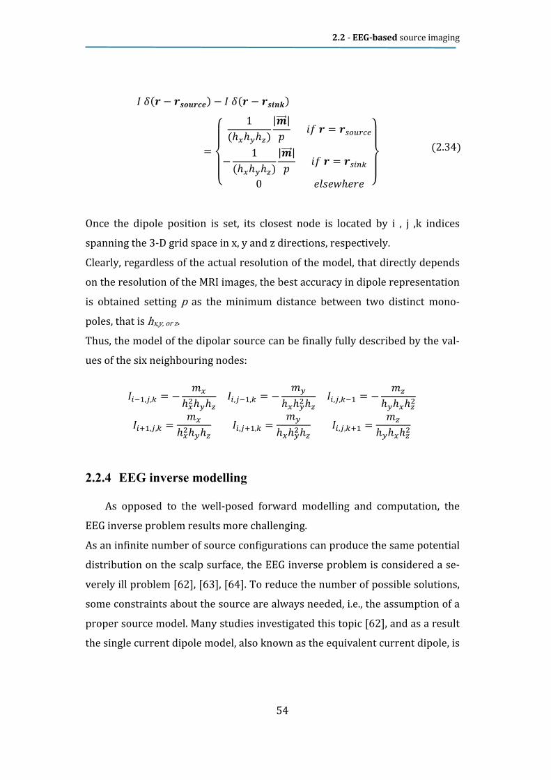
2.2 - EEG-based source imaging
54
Once the dipole position is set, its closest node is located by i , j ,k indices spanning the 3-D grid space in x, y and z directions, respectively. Clearly, regardless of the actual resolution of the model, that directly depends on the resolution of the MRI images, the best accuracy in dipole representation is obtained setting p as the minimum distance between two distinct mono-poles, that is hx,y, or z. Thus, the model of the dipolar source can be finally fully described by the val-ues of the six neighbouring nodes: � NJ,Î,¶ = − k}ℎ}Kℎ~ℎ� � ,ÎNJ,¶ = − k~ℎ}ℎ~Kℎ� � ,Î,¶NJ = − k�ℎ~ℎ}ℎ�K� õJ,Î,¶ = k}ℎ}Kℎ~ℎ� � ,ÎõJ,¶ = k~ℎ}ℎ~Kℎ� � ,Î,¶õJ = k�ℎ~ℎ}ℎ�K
2.2.4 EEG inverse modelling
As opposed to the well-posed forward modelling and computation, the
EEG inverse problem results more challenging. As an infinite number of source configurations can produce the same potential distribution on the scalp surface, the EEG inverse problem is considered a se-verely ill problem [62], [63], [64]. To reduce the number of possible solutions, some constraints about the source are always needed, i.e., the assumption of a proper source model. Many studies investigated this topic [62], and as a result the single current dipole model, also known as the equivalent current dipole, is
� �(� − �������) − � �(� − �����)=
ö÷ø÷ù 1(ℎ}ℎ~ℎ�) |�ZZZ[|ú jû � = �ªÂÃwüý
− 1(ℎ}ℎ~ℎ�) |�ZZZ[|ú jû � = �ª´�¶0 �iò�ðℎ�«� þ÷�÷� (2.34)

2.2 - EEG-based source imaging
55
the model that best fits for problems related to focal brain activity [65] and is used in this study. Furthermore, owing to the linearity of the forward problem, more complex activity can always be represented by superposition of a dipole distribution [66]. Several previous studies aimed to compare realistic geometry models to spherical models, focusing on their performances in source localisation (i.e., their application to the inverse problem). Although this is clearly a practical validation perspective, it is affected by the intrinsic uncertainties related to the particular source localization algorithm (inverse method) adopted. In fact, the imaging performance of all linear and nonlinear EEG inverse algorithms varies from case to case, depending on the nature of the brain electrical activity un-der analysis. Although the evaluation of some typical algorithms has been carried out in a few experimental and simulation settings, a general conclusion or agreement regarding a single optimal inverse approach, if at all possible, has not been reached [67]. In particular, the main issue to be addressed is the regularization problem. Referring to equation (2.16), all linear distributed inverse solutions can be expressed as a collection of many spatial filters (one per source dipole component and one per source position). Altogether, these spatial filters are applied to channel data for generating the estimated EEG/MEG source time-series in all source locations and for all source orientations: �� (c) = � ∙ ��(c) (2.35)
In this formulation, matrix WWWW contains all spatial filter weights (one weight per source dipole component and location and per channel) and �� (c) is the esti-mated source time-series for all components and locations. Assuming a mea-surement configuration with M channels, N sources and a free orientation model (i.e. X, Y and Z components are considered for each dipole), matrix WWWW has order 3*N*M.

2.2 - EEG-based source imaging
56
Since the orientation of the main EEG generators is orthogonal to the surface of the gray matter, as previously stated in section 2.2.1.2, it is common to con-strain the orientation of each source before the computation of the lead field matrix, that hence will result of order N*M. Similarly to the lead field matrix, the inverse solution matrix W W W W is stored as a collection of 3*M or M maps defined across all N source points depending on the orientation constrain. The estimation of the inverse solution W W W W can pro-ceed by either attempting a total inversion of the distributed ECD (DECD) model in (2.16) across the entire source space –the so called “imaging” ap-proach- or by filling three-by-three the rows of WWWW at each source location -“scanning” approach-. The problem of all imaging approach is that N >> M, and this makes the
linear problem severely ill-posed, i.e. no unique solutions exist if the only con-
strain is minimizing the residual term for fitting the measurements. Therefore,
besides the obvious mathematical constrain or minimizing the residual term in
(2.16), additional more “physical” constraints are to be posed to achieve a
unique solution.
2.2.4.1 Weighted Minimum -orm approach
One of the most popular “imaging” approach is the weighted minimum-
norm (WMN). The WMN compensates the lower gains of deeper sources by us-
ing lead field normalization. In this approach the weights in (2.35) are esti-
mated in such a way to produce the source distribution with the minimum
power that fits the measurements in a least-square-error sense:
Here, RRRR represents the “a priori” source covariance matrix and is used to “in-form” or “re-weight” the solution, i.e. to incorporate some prior knowledge
� = ��¢(���¢ + IK�)NJ ( 2 . 3 6 )

2.2 - EEG-based source imaging
57
about the spatial distribution of the source activity (RRRR=I I I I in case of no weight-ing). CCCCN N N N is the covariance matrix of the channel noise nnnn(t) in and is used to “regular-ize” the solution with respect to the actual noise distribution in the channel space. Assuming the noise spatially uniform across all channel sites corres-ponds to CCCCNNNN=IIII. The regularization parameter λ controls the amount of regularization in rela-tion to the expected SNR. Since minimum-norm solutions are intrinsically biased towards superficial source locations, a common weighting scheme called depth-weighting specifies R R R R as a diagonal matrix with non-zero entries inversely proportional to the γ–th power of lead field norms, with γ being the depth-weighting parameter: ´ = � (�)^,(L´õ^) (�)^,(L´õJ) (�)^,(L´õK)⋮ ⋮ ⋮(�)�NJ,(L´õ^) (�)�NJ,(L´õJ) (�)�NJ,(L´õK)� ( 2 . 3 7 )
(�)´Î ∶= Ó�´�NK (j = �)0 (j ≠ �)Õ
2.2.4.2 Laplacian-WM- and LORETA
An important variant of WMN is the Laplacian WMN which gives the
mathematical basis of the so-called Low-Resolution Electro-magnetic Topog-
raphic Analysis (LORETA) approach: (�)´Î = � 1 (j = �)
− 1���} (� ∈ � )0 �iò�Õ
� = ���(� ∙ �¢)NJ ( 2 . 3 8 )

2.2 - EEG-based source imaging
58
where Vi represents the set of nearest “neighbours” of the source location
at node i on the source space grid –or mesh- and Nmax the cardinal number of
Vi. Rdw is the same as in (2.37) and allows combining depth and spatial Lapla-
cian weighting, thus giving the depth-compensated inverse solution under the
constraint of smoothly distributed sources
2.2.4.3 Local Autoregressive Average
Local Autoregressive Average –or LAURA- weighting is similar to LORETA,
but the physical distances between sources dij are involved in the weighting
function and the cardinal number of Vi is allowed to vary across source loca-
tions: (�)´Î =
ö÷ø÷ù���}�´ ∙ · p´¶NK
¶��¿(j = �)
−p´ÎNK (� ∈ � )0 �iò�Õ
� = ���(� ∙ �¢)NJ ( 2 . 3 9 )
2.2.4.4 Spatial filter normalization
After estimation of the WMN spatial filter (2.36), some form of normaliza-
tion of the weights is usually applied. Dale et al. in [68] have proposed scaling
the filter weights at each source point by their variances in the channel space. (�)(L´õ�),Î → (�)(L´õ�),Î�∑ ∑ �(�)(L´õ�),¶�K�NJ¶Á^K�Á^
j = 0, … ,� − 1� = 0, … ,� − 1� = 0,1,2 ( 2 . 4 0 )
Applying this noise-based normalization has the important advantage of mak-
ing the point-spread function (PSF) of each source -i.e. the image of a point cur-
rent source placed in a given position- more uniform across the entire cortical
space, compared to the case of a minimum-norm solution without such nor-
malization.

2.2 - EEG-based source imaging
59
A variation of the noise-based normalization is the so-called standardized
LORETA or s-LORETA [69] that normalizes the inverse solution at each source
location using the resolution matrix T. More specifically, the set of filter
weights for the source at location i are jointly normalized using the i-th 3x3
block Ti along the diagonal of matrix T: Ì = � ∙ �Ì´ = �(Ì)(L´õ^),(L´õ^) (Ì)(L´õ^),(L´õJ) (Ì)(L´õ^),(L´õK)(Ì)(L´õJ),(L´õ^) (Ì)(L´õJ),(L´õJ) (Ì)(L´õJ),(L´õK)(Ì)(L´õK),(L´õ^) (Ì)(L´õK),(L´õJ) (Ì)(L´õK),(L´õK)
�
�´,Î = �(�)(L´õ^),Î(�)(L´õJ),Î(�)(L´õK),Î� j = 0, … ,� − 1� = 0, … ,� − 1
�´,Î → ÌNJ ∙ �´,Î
( 2 . 4 1 )
2.2.4.5 The regularization parameter
While weighting entails with applying data-independent mathematical and
physical constraints to an inverse solution, a regularization parameter (λ in
equation ( 2 . 3 6 )) is also introduced to avoid magnification of errors in data in
relation to signal-to-noise ratio (SNR). In fact, due to the ill-posed nature of the
problem of inverting the linear model in (2.16) for N > M, imaging approaches
always requires some form of regularization. A convenient formula can be
used to relate the regularization parameter to source SNR: I = c«ñe�(���¢)c«ñe�(��) ∙ ½��K ( 2 . 4 2 )
This formula allows adjusting the regularization in terms of a realistic guess for the signal-to-noise ratio (SNR) of the current sources. The lower the “guess” SNR, the higher the value of lambda that means less spatial resolution

2.2 - EEG-based source imaging
60
but higher sensitivity. The higher the “guess” SNR, the lower the value of lambda which means higher resolution but less sensitivity (i.e. we need higher SNRs to “resolve” a given source). Plotting the lambda values vs the SNR values normally provide a typical L-shaped curve. Ideally, one should choose the “knee” of this curve. 2.2.4.6 Scanning approaches: beamforming
Beamforming is a technique that performs a spatial filtering of signals
measured at discrete sensors [70]. Beamformers calculate a linear combina-
tion of the time sequences measured at the different sensors, with the aim of
preserving the signal components originating from a desired direction or loca-
tion, while at the same time suppressing interference from other directions or
locations. A typical application of beamforming is a spatial filtering of radar
signals, in which the signal in a certain direction-of-arrival is to be extracted
from the signals measured at a linear sensor array. Beamforming can be ap-
plied as well in cases with more general sensor configurations. In EEG, beamforming can be applied to implement a spatial filter that monitors the electrical activity in a certain brain region, while suppressing the contribu-tions of interfering activity in other regions. The behaviour of a beamformer in terms of spatial response function and sensitivity to noise is completely de-termined by the choice of its coefficients for linearly combining the input sig-nals. Different types of beamformers exist, depending on the criteria put forward to determine their coefficients. For instance, linearly constrained minimum variance (LCMVLCMVLCMVLCMV) beamformers [70] uses the following weight estimation for the source placed at location i:

2.3 - fMRI source imaging
61
�´ = � (�)^,(L´õ^) (�)^,(L´õJ) (�)^,(L´õK)⋮ ⋮ ⋮(�)�NJ,(L´õ^) (�)�NJ,(L´õ^) (�)�NJ,(L´õ^)�
�´ = �(�)(§�õÈ),È(�)(§�õË),È(�)(§�õ ),È… (�)(L´õ^),�NJ(�)(L´õJ),�NJ(�)(L´õK),�NJ
� → [(¢ ∙ �NJ) ∙ �´]NJ ∙ (�¢ ∙ �NJ)
Unlike ECD, beamforming does not require prior knowledge of the number
of sources, nor does it search for a solution in an underdetermined linear sys-
tem as does DECD.
For these reasons, beamforming remains the favourite method of many re-
searchers in electromagnetic source imaging and has been suggested for use in
the integrative analysis of E/MEG and fMRI.
2.3 fMRI source imaging
2.3.1 -eurovascular coupling and BOLD effect
Neuronal activity consumes energy, which is produced by chemical proc-
esses requiring glucose and oxygen. The vascular system supplies these sub-
stances by a complex network of large and small vessels.
A local increase of neuronal activity immediately leads to an increased
oxygen extraction rate in the capillary bed and, thus, in an increase in the rela-
tive concentration of deoxygenated haemoglobin. This response of the vascu-
lar system to the increased energy demand is called the hemodynamic re-
sponse. Still it is not completely known how the neurons inform the vascular
system about their increased energy demand. The most common method of fMRI is based on the Blood Oxygen Level-Dependent (BOLD) effect [71]. This exploits the fact that oxygenated haemog-

2.3 - fMRI source imaging
62
lobin has different magnetic properties to deoxygenated haemoglobin. More specifically, while oxygenated haemoglobin is diamagnetic, deoxygenated haemoglobin is paramagnetic altering the local magnetic susceptibility, creat-ing a magnetic field distortion within and around the blood vessels in the capil-lary bed and venules. The BOLD effect, thus measures increased neuronal ac-tivity indirectly via a change in local magnetic field (in) homogeneity, which is caused by an oversupply of oxygenated blood. Under the assumption of a linear time invariant (LTI) system, one can pre-
dict the expected time course of arbitrary long stimulation periods from the
known impulsive response. In the fMRI context the impulsive response is the
hemodynamic response function (HRF). The data analysis of almost all fMRI studies is therefore based on the signals coming from the sustained positive BOLD response. 2.3.2 Statistical analysis of functional data: GLM
Statistical data analysis aims at identifying those brain regions exhibiting
increased or decreased responses in specific experimental conditions as com-
pared to other (e.g. control conditions). Due to the presence of physiological
and physical noise fluctuations, observed differences between conditions
might occur simply by chance. The statistical data analysis assesses the effect
of noise fluctuations on estimated condition differences. In standard fMRI
analyses this assessment is performed independently for the time course of
each voxel. The obtained statistical values, one for each voxel, form a 3-D sta-
tistical map. In more complex analyses each voxel will contain several statisti-
cal values rejecting estimated effects of multiple conditions.
Without entering into details of such complex and advanced statistical meth-
ods, we will limit to cite the main analysis techniques used in this study: the
general linear model (GLM). In a GLM analysis the data is processed voxel-wise
(univariate) by fitting a model to the time course of each voxel independently

2.3 - fMRI source imaging
63
In order to effectively describe the method, let us first give a brief overview of
few statistical concepts.
2.3.2.1 Statistical mean comparison
Statistical analysis essentially asks how likely it is to obtain a certain effect
if there would be only noise fluctuations. This is formalized by the null hy-
pothesis stating that there is no effect, i.e. no difference between conditions.
Assuming the null hypothesis, it can be calculated how likely it is that an ob-
served effect would have occurred simply by chance. This requires knowledge
about the amount of noise fluctuations which can be estimated from the data.
By incorporating the variability of measurements, statistical data analysis al-
lows to estimate the uncertainty of effects (e.g. mean differences) in data sam-
ples. If an effect is so large that it is very unlikely that it has occurred simply by
chance (e.g. the probability is less than p = 0.05), one rejects the null hypothe-
sis and accepts the alternative hypothesis stating that there exists a true effect.
2.3.2.2 t Test
The uncertainty of an effect is estimated by calculating the variance of the
noise fluctuations from the data. For the case of comparing two mean values,
the observed difference of the means is related to the variability of that differ-
ence resulting in a t statistic:
c = !Kµµµ − !Jµµµ|�"#µµµµN"$µµµµ
The numerator is the mean difference while the denominator is the estimate of the expected variability, the standard error of the mean difference. Estimation of the standard error involves pooling of the variances obtained within both conditions. The higher the t value, the less likely it is that the observed mean difference is just the result of noise fluctuations. It is obvious that measurement of many data points allows a more robust estimation of this probability than the mea-

2.3 - fMRI source imaging
64
surement of only a few data points. The error probability p can be calculated exactly from the obtained t value using the incomplete beta function Ix(a,b) and the number of measured data points N: ú = � �NK�NKõÄ# � − 22 , 12®
If the computed error probability falls below the standard value (p < 0.05), the alternative hypothesis is accepted stating that the observed mean difference exists in the population from which the data points have been drawn (i.e. measured). In that case, one also says that the two means differ significantly. 2.3.2.3 Correlation Analysis
The described mean comparison method is not the ideal approach to com-
pare responses between different conditions since this approach is unable to
capture the gradual profile of fMRI responses. As long as the temporal resolu-
tion is low (volume-TR > 4 seconds), the mean of different conditions can be
calculated easily because transitions of expected responses from different
conditions occur within a single time point. If the temporal resolution is high
(e.g., 2 seconds), the expected fMRI responses change gradually from one con-
dition to the next due to the sluggishness of the hemodynamic response. In this
case, time points cannot be assigned easily to different conditions. Without
special treatment, the mean response can no longer be easily computed for
each condition. As a consequence, the statistical power to detect mean differ-
ences may be substantially reduced, especially for short blocks and events.
To overcome this problem the correlation analysis is used, since this
method allows explicitly incorporating the gradual increase and decrease of
the expected BOLD signal. A predicted gradual time courses is used as the ref-
erence function in a correlation analysis. At each voxel, the time course of the

2.3 - fMRI source imaging
65
reference function is compared with the time course of the measured data by
calculation of a correlation coefficient r, indicating the strength of co variation: « = ∑ (!Ä − !µ)(&Ä − &µ)�ÄÁJf∑ (!Ä − !µ)K�ÄÁJ ∑ (&Ä − &µ)K�ÄÁJ
Index t runs over time points (t for “time”) identifying pairs of temporally cor-responding values from the reference (Xt) and data (Yt) time courses. The term in the denominator normalizes the covariation term in the numerator so that the correlation coefficient lies in a range of -1 and +1. A value of +1 indicates that the reference time course and the data time course go up and down in ex-actly the same way, while a value of -1 indicates that the two time courses run in opposite direction. A correlation value close to 0 indicates that the two time courses do not covary, i.e. the value in one time course cannot be used to pre-dict the corresponding value in the other time course. Since the reference function is the result of a model assuming different re-sponse strengths in the two conditions (e.g. “Rest” and “Stim”), a significant correlation coefficient indicates that the two conditions lead indeed to differ-ent mean activation levels in the respective voxel. 2.3.2.4 General linear model
The General Linear Model (GLM) is mathematically identical to a multiple
regression analysis but stresses its suitability for both multiple qualitative and
multiple quantitative variables. Because of its flexibility to incorporate multi-
ple quantitative and qualitative independent variables, the GLM has become
the core tool for fMRI data analysis after its introduction into the neuroimag-
ing community by Friston et al. [72, 73]. In its general form, the General Linear
Model has been defined for multiple dependent variables, i.e. it encompasses
tests as general as multivariate covariance analysis (MANCOVA).

2.3 - fMRI source imaging
66
From the perspective of multiple regression analysis, the GLM aims to
predict the variation of a dependent variable in terms of a weighted sum of
several reference functions. The dependent variable corresponds to the ob-
served fMRI time course of a voxel and the reference functions correspond to
time courses of expected fMRI responses for different conditions of the ex-
perimental paradigm.
The reference functions are also called predictors, regressors, explanatory
variables, covariates or basis functions. A set of specified predictors forms the
design matrix, also called the model. A predictor time course is typically ob-
tained by convolution of a condition box-car time course with a standard
hemodynamic response function (two-gamma HRF or single-gamma HRF). A
condition box-car time course may be defined by setting values to 1 at time
points at which the modelled condition is defined (“on”) and 0 at all other time
points.
Each predictor time course X gets an associated coefficient or beta weight b,
quantifying its potential contribution in explaining the voxel time course y. The
voxel time course y is then modelled as the sum of the defined predictors, each
multiplied with the associated beta weight b. Since this linear combination will
not perfectly explain the data due to noise fluctuations, an error value e is
added to the GLM system of equations with N data points and p predictors: äJ = '^ + 'J!JJ + ⋯ + 'v!Jv + �J⋮ä� = '^ + 'J!�J + ⋯ + 'v!�v + �� Where the y variable on the left side corresponds to the data. After estimation (see below), the value of b0 typically represents the signal level of the baseline condition, also called intercept.

2.4 - EEG-fMRI integration
67
While its absolute value is not informative, it is important to include the con-stant predictor in a design matrix since it allows the other predictors to model small condition-related fluctuations as increases or decreases relative to the baseline signal level. The other predictors on the right side model the expected time courses of different conditions. For multi-factorial designs, predictors may be defined coding combinations of condition levels in order to estimate main and interaction effects. The beta weight of a condition predictor quanti-fies the contribution of its time course in explaining the voxel time course. While the exact interpretation of beta values depends on the details of the de-sign matrix, a large positive (negative) beta weight typically indicates that the voxel exhibits strong activation (deactivation) during the modelled experi-mental condition relative to baseline. All beta values together characterize a voxels “preference” for one or more experimental conditions. The last column in the system of equations contains error values, also called residuals, predic-tion errors or noise. These error values quantify the deviation of the measured voxel time course from the predicted time course, the linear combination of predictors. In vectors and matrices notation, the last equation can be written as: ( = )* + � Thus leading to a classic linear problem that can be solved in a least square sense....
2.4 EEG-fMRI integration
The integration of EEG/MEG and fMRI works under the hypothesis that
the regions with the greater fMRI BOLD responses have a larger possibility of
being electrically active over the time period of interest [74], [75], [68].
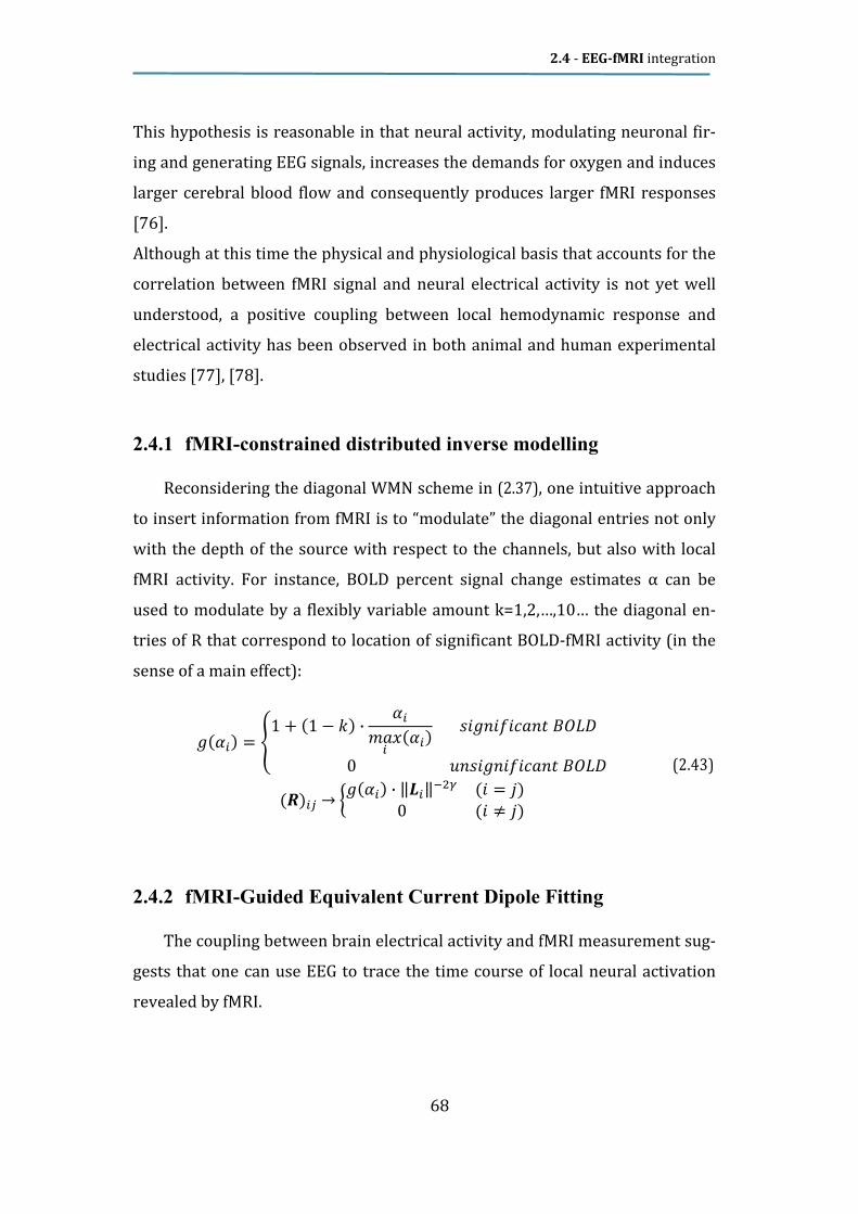
2.4 - EEG-fMRI integration
68
This hypothesis is reasonable in that neural activity, modulating neuronal fir-ing and generating EEG signals, increases the demands for oxygen and induces larger cerebral blood flow and consequently produces larger fMRI responses [76]. Although at this time the physical and physiological basis that accounts for the correlation between fMRI signal and neural electrical activity is not yet well understood, a positive coupling between local hemodynamic response and electrical activity has been observed in both animal and human experimental studies [77], [78]. 2.4.1 fMRI-constrained distributed inverse modelling
Reconsidering the diagonal WMN scheme in (2.37), one intuitive approach
to insert information from fMRI is to “modulate” the diagonal entries not only
with the depth of the source with respect to the channels, but also with local
fMRI activity. For instance, BOLD percent signal change estimates α can be
used to modulate by a flexibly variable amount k=1,2,…,10… the diagonal en-
tries of R that correspond to location of significant BOLD-fMRI activity (in the
sense of a main effect): +(,´) = ï1 + (1 − -) ∙ ,´kñÜ´ (,´) òj+�jûjeñ�c `ßF
0 Û�òj+�jûjeñ�c `ßFÕ(�)´Î → Ó+(,´) ∙ ��´�NK (j = �)0 (j ≠ �)Õ (2.43)
2.4.2 fMRI-Guided Equivalent Current Dipole Fitting
The coupling between brain electrical activity and fMRI measurement sug-
gests that one can use EEG to trace the time course of local neural activation
revealed by fMRI.
2.4 - EEG-fMRI integration
69
The activation foci derived from fMRI images can be used to guide the place-ment of dipole locations, and the dipole orientation and strength are then fit-ted so as to best explain the observed bioelectromagnetic measurements over the time period of the relative neural process. Modified from this procedure is a technique of “fMRI-seeded dipoles,” which only uses the fMRI foci as initial guesses (or seeds) for dipole locations and ad-justs the dipole parameters using nonlinear optimization algorithms [79], [80]. In some cases, these techniques lead to a significant conclusion in resolv-
ing the timing details of localized activation and the interactions across differ-
ent neuron assemblies that cannot be obtained when using fMRI alone. On the
other hand, the fMRI-guided initial guess of dipole locations has largely allevi-
ated the local minima problem inherent in nonlinear optimization procedures
that may have been experienced in traditional multiple dipole fitting problems
solely based on EEG or MEG.
Because the conventional fMRI techniques aided by these ECD-based ap-
proaches can provide additional temporal information beyond identifying the
locations of neural activation, they have the potential to reveal the dynamic
neuronal events, which can hardly be achieved by fMRI alone. However, these
techniques are always limited by their inability to resolve complex spatiotem-
porally distributed activities, which are usually induced by a high-level cogni-
tive task. When a large extent of neuronal network is active in parallel, the ap-
plicability of a simple dipole model would be questionable; or when a large
number of different brain regions are involved, the nonlinear fitting procedure
may fail to reach an optimal solution.
2.4.3 fMRI-Constrained Cortical Current Imaging
In order to account for the distributed nature of the neural sources inside
the brain, fMRI has also been incorporated in the estimation of the continuous
distribution of cortical current density. In this approach, fMRI data are used to

2.4 - EEG-fMRI integration
70
bias the EEG/MEG inverse solution towards those locations deemed statisti-
cally significant in the view of fMRI [78], [75].
This can be implemented under different mathematical frameworks, such as:
1) in the context of the generalized Wiener filtering, which states that an opti-
mal linear estimator can be derived given the covariance matrices of both
source and sensor noise, fMRI spatial information is encoded into the diagonal
elements of source covariance matrix [68], [75];
2) Based on the regularization strategy of generalized weighted minimum
norm, one can set the weight matrix according to the fMRI significance, or p-
value, to allow for the fMRI preference [74]. It is worth pointing out that these
two frameworks are fundamentally equivalent, as we can see with the Wiener
estimator n = �¢(�¢ + .)NJ ( 2 . 4 4 )
where L is the lead field matrix, C the sensors noise covariance matrix, and R a source covariance matrix derived from fMRI activation maps. Since a voxel in fMRI must be either active or inactive, the fMRI-derived source covariance can be written as � = �/ ∙ I ( 2 . 4 5 )
where the diagonal elements of Rf are set to a positive value f only for those dipoles whose locations are deemed active in fMRI, while other diagonal ele-ments are set to 1, and λ is a regularization parameter. The inverse operator as (2.45) is also the minimiser of a generic weighted minimum norm function 0 = 1.NJK(' − åÜ)1KK + 1« 2�/NJ/KÜ2K
K ( 2 . 4 6 )
2.4 - EEG-fMRI integration
71
The parameter f controls the amount of bias towards fMRI active locations, which depends on the confidence in our hypothesis that neuronal and hemo-dynamic activities are collocated. The regularization parameter r can either be determined by standard ap-proaches like “L-curve” or be calculated if the noise covariance C is accurately estimated [81]. A further refinement of this technique is to quantitatively con-sider the reliability of source estimation with respect to the effect of sensor noise. Due to the linearity of both forward and inverse operators, the fMRI-constrained current density estimation can be normalized by the noise sensi-tivity, yielding unit-free dynamic statistical parametric maps (dSPM) of brain activity [68]. Furthermore, some of the latest advances have been made to estimate the
connectivity patterns among different cortical regions of interest (ROIs) using
the estimated cortical current density via directed transfer function (DTF) [82]
or structural equation modelling [83]. Cortical connectivity estimation pro-
vides an important perspective regarding the causal relation and information
flow pathways and, thus, specifically addresses how neuronal assemblies are
activated and coordinated. Notably, a recent study on cortical connectivity es-
timation based on the combination of EEG and fMRI has been reported [82].
The high-density EEG as well as MRI/fMRI data were collected in separate ex-
aminations when the same subject was performing the same visually triggered
finger-tapping task.
By using the linear inverse operator constrained by fMRI, the cortical cur-
rent density was noninvasively estimated from EEG and then averaged to de-
velop representative waveforms for preselected ROIs. DTF technique was ap-
plied to estimate the directional causality in various frequency bands among
different ROIs, and the connectivity pattern was visualized in a subject-specific
cortex reconstructed from MRIs

2.4 - EEG-fMRI integration
72
2.4.4 Multimodal Beamforming
Lahaye et. al. [84] suggest an iterative algorithm for conjoint analysis of
EEG and fMRI data acquired simultaneously during an event-related experi-
ment. Their method relies on iterated source localization by the LCMV beam-
former, which makes use of both EEG and fMRI data. The covariance CX used by
the beamformer is calculated anew each time step, using the previously esti-
mated sources and current event responses from both modalities.
This way neuronal sites with a good agreement between the BOLD response
and EEG beamformer reconstructed source amplitude, benefit most at each it-
eration.
Although the original formulation is cumbersome, this method appears
promising as (a) it makes use of both spatial and temporal information avail-
able from both modalities, and (b) it can account for silent BOLD sources using
an electro-metabolic coupling constant which is estimated for each dipole and
defines the influence of the BOLD signal at a given location onto the estimation
of CS which, in turn, drives the estimate of CX.
2.4.5 EEG Source Analysis with EEG-fMRI Coupling
Exploring the signal coupling of simultaneously recorded EEG and fMRI
time-series is attractive because fMRI signals can be automatically predicted
(and fMRI patterns can be generated) directly from spatio-temporally selective
EEG responses, thus improving accuracy in source localization [85].
2.4.5.1 Background
Modeling EEG-fMRI coupling effects entails with the extraction of inte-
grated features from the EEG source responses, e.g. the EEG source power at a
given latency or inside a given time or time-frequency interval. The resulting
series of “EEG values” is then standardized across all trials and converted to a
new time-course at the fMRI temporal resolution (TR). The conversion from

2.4 - EEG-fMRI integration
73
this series of EEG measures to an fMRI predictor is performed in two steps: (i)
hemodynamic convolution at EEG time resolution and (ii) time-course resam-
pling at fMRI time resolution. The resulting time-course can be used for pre-
dicting and modeling, and, hence, localizing the joint fluctuations of EEG and
fMRI signals.
2.4.5.2 Processing
The series of EEG values is standardized (i.e. the mean is subtracted and
the values are scaled to their standard deviation) and convolved with the dou-
ble gamma hemodynamic function estimated at the EEG time resolution and
resampled at the fMRI time resolution. Assuming a series of N EEG values (cor-
responding to N EEG epoch-specific measures, either from stimulus or fMRI
triggers) and a series of K fMRI values (corresponding to T fMRI time points),
the EEG-fMRI coupling time-course can be easily expressed as a discrete time
convolution:
ä(-) = · YYn� ∙ 3�4(c¶ − c�) - = 1,2 … … .5��ÁJ
Where: EEGn is the integrated measure corresponding to the n-th trial tn is the time of n-th trial trigger (with respect to the EEG segment) tk is the time of the k-th fMRI trigger (with respect to the EEG segment) HRF(t) is the hemodynamic response function Hemodynamic convolution at the original EEG resolution is necessary because
the stimulus or any other EEG trigger of interest is normally not synchronized
with all fMRI time points, with the sole exception of the fMRI trigger itself. On
the other hand, even if the fMRI trigger is used to extract EEG values, the long
fMRI repetition time (normally 100:1000 times longer than the EEG sampling
period) may suggest using different subintervals within each TR with the re-
sult of introducing a time shift between the trigger event and the actual EEG
measure.

2.4 - EEG-fMRI integration
74
2.4.5.3 Experimental note
When analyzing simultaneous EEG-fMRI data, there are two alternative approaches for extracting the series of EEG values to be used in the prediction and modeling of the fMRI data: single-trial coupling and continuous coupling. Single-trial coupling entails with extracting EEG features from each single-trial response (e.g. the power at a certain latency or inside a given time-frequency box) with respect to the stimulus trigger; these values are assumed to be ca-pable of modulating the amplitude of the event-related fMRI response to that stimulus. Continuous coupling entails with integrating the EEG power inside a certain time-frequency box defined with respect to the fMRI trigger. In general, the choice between these two approaches is implicitly driven by the experi-mental design. In event-related designs a single EEG trigger of a given protocol condition is associated with the occurrence of single experimental stimulus whose dura-tion is assumed to be zero (i.e. an impulse). Assuming that the absence of a stimulus implies the absence of a neuronal response and, vice versa, the pres-ence of a stimulus implies the presence of the fMRI response, the EEG-fMRI coupling for that condition can be studied directly from single-trial data (STD/TFD) prepared for that specific stimulus. In block-design experiments a single stimulus trigger only defines the on-set or the offset of a block (or, equivalently, the borders of a data segment). In this case, the fMRI trigger should be used and an integrated EEG measure (e.g. the total power in a given frequency band) is calculated for each TR. More in general, this approach is preferred in all cases where EEG-fMRI correlations are studied for long periods corresponding to entire segments rather than short trials of EEG data (e.g. resting-state, free viewing or listening, etc.).

3.1 - Aim of the study
75
3 Comparative analysis of different head modelling ap-
proaches in EEG-based functional neuroimaging
3.1 Aim of the study
So far, it is not yet clear which brain regions are more sensitive to the
choice of different model geometry, both from quantitative and qualitative
point of view. In order to address this issue and avoiding the intrinsic uncer-
tainties related to the particular inverse method adopted [67], we propose a
comparison between the effects that different modelling approaches directly
give on the forward fields [44], [34]. One is the anatomically-shaped modelling
approach, the other is the well known multi-layer spherical geometry ap-
proach. This knowledge would allow determining whenever the spherical ap-
proximation shall meet the required accuracy for the EEG current sources un-
der investigation. In order to achieve as much generality as possible, we based
our study on the MNI152 template, since it is derived from an average of sev-
eral healthy humans head MRIs; hence the inferred considerations shall be
widely applicable [59]. Starting from real magnetic resonance imaging (MRI)
high-resolution anatomical images we explore the spatial variation of the for-
ward fields, directly basing on the analysis of the lead fields [34] produced by
simulated cortical sources placed on the reconstructed mesh of the neocortex
along the surface electrodes of a 62-channel configuration. We first proposed a comparison between realistic and approximated geome-try, whose results have been published in [6], then we decided to deepen the study including two distinct approaches of realistic modelling [7]

3.2
with one more electrode acting as reference (
brain cortex surface from the averaged MNI head and brain image dataset
(Figure
ferred to as our
sible source positions. The three orthogonal dipole orientation axes are d
rected as follows: right
axis).
3.3
helpful in EEG source analysis even when only EEG and no specific MRI data
are available for a particular subject, or the acquired dataset was not suitable
for segmentation. In these cases, a lead field
3.2 Sensors and sources
We started considering a typical 62
with one more electrode acting as reference (
brain cortex surface from the averaged MNI head and brain image dataset
Figure 3-1 on the left), subsampled to 5000 vertices. The latter will be r
ferred to as our
sible source positions. The three orthogonal dipole orientation axes are d
rected as follows: right
axis).
3.3 Building of the M-I
model
We aimed to develo
helpful in EEG source analysis even when only EEG and no specific MRI data
are available for a particular subject, or the acquired dataset was not suitable
for segmentation. In these cases, a lead field
Figure 3-1Left: Brain cortex mesh representing the s
Sensors and sources
We started considering a typical 62
with one more electrode acting as reference (
brain cortex surface from the averaged MNI head and brain image dataset
on the left), subsampled to 5000 vertices. The latter will be r
ferred to as our source space
sible source positions. The three orthogonal dipole orientation axes are d
rected as follows: right-left (
Building of the M-I
model
We aimed to develo
helpful in EEG source analysis even when only EEG and no specific MRI data
are available for a particular subject, or the acquired dataset was not suitable
for segmentation. In these cases, a lead field
Left: Brain cortex mesh representing the s
Sensors and sources
We started considering a typical 62
with one more electrode acting as reference (
brain cortex surface from the averaged MNI head and brain image dataset
on the left), subsampled to 5000 vertices. The latter will be r
source space, i.e., the surface the vertices of
sible source positions. The three orthogonal dipole orientation axes are d
left (x axis), frontal
Building of the M-I
We aimed to develop a generic realistic geometry template that could be
helpful in EEG source analysis even when only EEG and no specific MRI data
are available for a particular subject, or the acquired dataset was not suitable
for segmentation. In these cases, a lead field
Left: Brain cortex mesh representing the s
scalp surface, represented by the spheres
76
Sensors and sources
We started considering a typical 62-channel EEG electrode configuration,
with one more electrode acting as reference (
brain cortex surface from the averaged MNI head and brain image dataset
on the left), subsampled to 5000 vertices. The latter will be r
, i.e., the surface the vertices of
sible source positions. The three orthogonal dipole orientation axes are d
axis), frontal-occipital (
Building of the M-I-template
p a generic realistic geometry template that could be
helpful in EEG source analysis even when only EEG and no specific MRI data
are available for a particular subject, or the acquired dataset was not suitable
for segmentation. In these cases, a lead field
Left: Brain cortex mesh representing the source space. Right: the electrodes positions on
scalp surface, represented by the spheres
channel EEG electrode configuration,
with one more electrode acting as reference (Figure 3
brain cortex surface from the averaged MNI head and brain image dataset
on the left), subsampled to 5000 vertices. The latter will be r
, i.e., the surface the vertices of
sible source positions. The three orthogonal dipole orientation axes are d
occipital (y
template-based
p a generic realistic geometry template that could be
helpful in EEG source analysis even when only EEG and no specific MRI data
are available for a particular subject, or the acquired dataset was not suitable
for segmentation. In these cases, a lead field computation performed on this
ource space. Right: the electrodes positions on
scalp surface, represented by the spheres
3.2 - Sensors
channel EEG electrode configuration,
3-1 on the right)
brain cortex surface from the averaged MNI head and brain image dataset
on the left), subsampled to 5000 vertices. The latter will be r
, i.e., the surface the vertices of which are all po
sible source positions. The three orthogonal dipole orientation axes are d
axis) and bottom
based realistic
p a generic realistic geometry template that could be
helpful in EEG source analysis even when only EEG and no specific MRI data
are available for a particular subject, or the acquired dataset was not suitable
computation performed on this
ource space. Right: the electrodes positions on
Sensors and sources
channel EEG electrode configuration,
he right), and a
brain cortex surface from the averaged MNI head and brain image dataset
on the left), subsampled to 5000 vertices. The latter will be r
which are all po
sible source positions. The three orthogonal dipole orientation axes are d
axis) and bottom-up (
realistic
p a generic realistic geometry template that could be
helpful in EEG source analysis even when only EEG and no specific MRI data
are available for a particular subject, or the acquired dataset was not suitable
computation performed on this
ource space. Right: the electrodes positions on
d sources
channel EEG electrode configuration,
, and a
brain cortex surface from the averaged MNI head and brain image dataset
on the left), subsampled to 5000 vertices. The latter will be re-
which are all pos-
sible source positions. The three orthogonal dipole orientation axes are di-
up (z
p a generic realistic geometry template that could be
helpful in EEG source analysis even when only EEG and no specific MRI data
are available for a particular subject, or the acquired dataset was not suitable
computation performed on this

3.3 - Building of the MNI-template-based realistic model
77
model and based on the real EEG sensors locations can be used to perform
source analysis.
A realistic-shaped FDM volume conductor model of the head was derived from
an averaged T1-weighted MRI dataset, available from the Montreal Neurologic
Institute (http://www.mni.mcgill.ca/). Segmentation by BrainSuite analysis tool (http://brainsuite.usc.edu/) was used to identify the following five tissue types in the head: scalp, skull, cere-brospinal fluid (CSF), gray matter, and white matter (see Figure 3-2).
In addition to the standard three compartments of scalp, skull, and brain, the CSF layer has been considered as it plays an important role in modifying the scalp potentials and can also influence the inverse source localizations [86] .
Figure 3-2(a), (b), and (c): Realistic FDM model based on the M7I anatomy composed by four compartments
representing scalp (pink), skull (green), CSF (blue), and brain, given by fusion of grey matter and white matter.
(d): The complete 3D model, with rendered surfaces.

3.3 - Building of the MNI-template-based realistic model
78
Based on literature [87], we set the homogeneous isotropic conductivities as σ = 0.33 S/m (skin), σ = 0.0042 S/m (skull), σ = 1.0 S/m (CSF), σ = 0.33 S/m (GM), and σ = 0.14 S/m (WM), respectively Moreover, aiming to assess the influence that tissue anisotropy has on EEG
forward modeling, we proceeded in characterize white matter and skull bones
tissue conductivity tensors. The following paragraphs will describe the overall
implemented process to build an anisotropy template for white matter and
skull bones.
3.3.1 Workflow overview
The following key points briefly summarise the steps necessary to build
the template, before describing each step in detail:
• Selection of DTI datasets • Pre-processing: • Eddy currents correction for all subjects • Brain Extraction Tool (BET) • Extraction of DTI components (DTIFIT) • Application of VBM-style process for gray matter alignment • Application of TBSS-style process for white matter alignment • Application of TBSS-style NON FA process for computation of eigenva-lues of final template • Implementation of vectorial registration and alignment procedures preceding averaging to calculate the eigenvectors of the final template • Computation of diffusion tensor matrices

3.3 - Building of the MNI-template-based realistic model
79
As the conductivity tensors are assumed to share the same eigenvalues
and eigenvectors of diffusion tensors, we start considering the diffusion ten-
sors analysis
RAW DATA
PREPROCESSING
APPLY WARP TO SELECTED FA
IMAGE , THIS IS REFERENCE IN
TBSS PROCESS
TBSS PROCESS TO CALCULATE
THE TEMPLATE FA IMAGE
TBSS NON FA PROCESS TO
CALCULATE THE EIGENVAL-
UES TEMPLATE IMAGES
(L1,L2 AND L3)
APPLY WARP TO EIGENVECTORS
IMAGES (V1, V2, V3)
APPLY AVARAGE-VECTORS TO CAL-
CULATE THE V1,V2 AND V3 EIGEN-
VECTOR TEMPLATE IMAGES
BUILD OF TEMPLATE DIFFU-
SOR TENSOR IMAGE
EDDY CURRENTS
CORRECTION
BRAIN EXTRAC-
TION TOOL
FITS THE DIFFU-
SION TENSOR
MODEL (DTIFIT)
FSL_VBM PROCESS TO
FIND TARGET SUBJECT
T1 DATA
bvals,
bvecs

3.3 - Building of the MNI-template-based realistic model
80
Most of the mentioned steps have been performed using the FSL software
package [88], [89] which includes many DWI/DTI processing tools.
3.3.2 DWI Data
The data sets used in this work have been made available by the John
Hopkins University Medical Institute, Laboratory of Brain Anatomical MRI,
with a DTI database which has been developed under the Human Brain Project
and National Research Resource Center grant. We used a group of twenty raw
DTI datasets of normal population; each of them is composed by three studies
with the same acquisition protocol. The data are anonymous with the follow-
ing imaging characteristics: All dataset have been acquired by means of a 1.5 T Philips MRI scanner Scan mode Multiple slice Number of slice 50 Scan resolution (x, y) 96 96 Recon resolution (x, y) 256 256 FOV (ap,fh,rl) [mm] 240.00 125.00 240.00 Slice thickness [mm] 2.50 Slice gap [mm] 0.00 Data Format Analyze Gradient directions 35 B value [s/mm2] 700
3.3.3 Voxel Based Morphometry procedure
Once artefacts (eddy currents and head motion) correction have been car-
ried out, we applied DTIFIT tool to fit the diffusion tensor to each voxel, thus

3.3 - Building of the MNI-template-based realistic model
81
obtaining L1, L2, L3 (the eigen values), V1, V2, V3 (the eigenvectors) that fully
describe each tensor.
In order to align all the Grey Matter (GM) images, these need to be first
transformed into a standard space, which involves the use of non-linear regis-
tration. This approach is somewhat of a trade-off: all the cortex morphologic
features across subjects are desirable to match, but not "too much" or one
would not be able to see any difference, if all these structures were perfectly
aligned across the subjects. That's why we use limited degrees-of-freedom for
the non-linear registration.
Structural data have been analysed by means of FSL VBM-style analysis facili-
ties, which perform brain-extraction of structural images applying BET, and
tissues segmentation with the FAST tools provided by FSL.
The resulting grey-matter partial volume images were then aligned to MNI152
standard space using the affine registration tool FLIRT, followed by nonlinear
registration using FNIRT towards the GM-ICBM-152 template.
3.3.4 Target subject and template determination
At the end of the process described above, we use the information pertain-
ing to the warp matrices for selecting the subjects’ reference. We have a num-
ber of related files that is equal to the number of subjects; these files are char-
acterized by two important parameters: the mean of the squared mean values
across the three images of warp volume (computed on non-zero voxels) and
the percentile of 50% of the squared mean values across the three images of
warp volume (that is the median). We use this information to select the best
target subject. The warp files are then compared to find the target that re-
quires the minimal changes to get warped into the MNI standard space (with
reference to GM-ICBM 152), i.e., the subject more similar to the MNI template.
Once identified the best target subject, in the second part of the code, the
same warping to standard space is applied on best target subject’s FA maps.

3.3 - Building of the MNI-template-based realistic model
82
Finally, this results in the target image, that we call TEMPLATE_FA, in the final
standard space.
3.3.5 Application of Tract Based Spatial Statistics (TBSS)
Voxelwise statistical analysis of the FA data was carried out using TBSS
(Tract-Based Spatial Statistics, [90]), part of FSL [89].
First, FA images were created by fitting a tensor model to the raw diffusion
data using FDT, and then brain-extracted using BET. All subjects' FA data were
then aligned into the common space TEMPLATE_FA using the nonlinear regis-
tration tool FNIRT, which uses a b-spline representation of the registration
warp field. Hence, the warp matrix obtained projects each subject’s data into
the MNI152 space. This warp matrix will be later applied to the eigenvectors
images.
Next, the mean FA image was created and thinned to create a mean FA
skeleton which represents the centres of all tracts common to the group. Each subject's aligned FA data was then projected onto this skeleton and the resulting data fed into voxelwise cross-subject statistics. Finally, we threshold the skeleton images to create a mask, and create a skele-ton distance map projecting all FA data onto the skeleton. FA data have been threshold at 0.2. We applied this technique also to each eigenvalues map and then averaging the results across the subjects in order to obtain the eigenvalues template. 3.3.6 Eigenvectors estimation
The final step of the overall process consists in estimating a sort of vector
averaging across the subject’s eigenvectors maps previously computed.

3.3 - Building of the MNI-template-based realistic model
83
First, the warping matrix computed during the previous FNIRT processing is applied to warp all the eigenvectors towards the “best target”. Then, a second transform warps the vectors to the FMRIB58 model into MNI152 space. Eventually, with all the vectors in template standard space, we can estimate the mean value of eigenvectors for each voxel by averaging, estimating their orientation’s mode. Since in each voxel of the final image the eigenvectors orientations of all subjects must be taken into account and since all of them can reasonably be assumed affected from noise, especially in the non-white-matter voxels, a simple vectors averaging could lead to poorly reliable results. This is why the mode (across the subjects) of the orientations of each eigenvector has been taken into account. Figure 3-3 illustrates the FA image with the usual col-or-coding referred to the first eigenvector:
Figure 3-3 FA image with V1 color-coding, tri-axial view

3.3 - Building of the MNI-template-based realistic model
84
3.3.7 From conductivity tensors to diffusion tensors
As already stated DT-MRI doesn’t measure conductivity tensor directly but
rather infers from the diffusion tensors which describes the movement of both
water molecules and electrically charged particles (ions). To implement conductivity tensor we assume that the same structural features that result in anisotropic mobility of water molecules also result in anisotropic conductivity. In other words the eigenvectors of the conductivity tensor can be considered similar as those from water diffusion tensor Furthermore the eigenvalues can be estimated from the isotropic conductivity by means of two constraints, whose effectiveness has been proven in white matter anisotropy measurements: ï43 ¤|7Â�8�|7Â�8�K = 43 ¤|´ªÂL
|7Â�8 ∙ |Äw��ª = |´ªÂK Õ They are called volume constraint [87] and Wang’s constraint [91], respective-ly. Figure 3-4 below shows the result of the white matter conductivity tensor im-
aging: Figure 3-4 Conductivity tensor imaging. Left: axial view, Right: detailed view. The image in background is the
FA image

3.3 - Building of the MNI-template-based realistic model
85
3.3.8 Skull conductivity anisotropy
Realistic modelling of the conductivity tensor eigenvalues in the skull is a
difficult task, not only because the absolute and relative thicknesses of
spongiosa and compacta layers vary and their boundaries are difficult to seg-
ment, but especially because of inhomogeneous skull resistivity and an inter-
and intrasubject variability which can be related to age, diseases, environ-
mental factors, and personal constitution [92], [93]. We therefore started from the commonly used isotropic conductivity value of skull = 0.0042 S/m [94], and assumed a given anisotropy ratio σ9:;<: σ=>?@A =1: 10 according to [93], [66], [25]. Next we applied Wang’s constraint which has been proven to lead to smaller errors, according to [87]. 3.3.9 Effects of anisotropy in Lead Field computation
In order to assess the effects that conductivity anisotropy has on the for-
ward modelling, we directly cross-compared four LF matrices, one of them
based on an fully-isotropic modelling, and the other computed with a different
anisotropy characterization (white matter only, skull only, both), by means of a
correlation of the LF values (see section 3.6.3). The first two models compared to the isotropic one present anisotropy charac-terization either of the only white matter conductivity, or the only skull bones conductivity. These two results are illustrated in Figure 7-10a and Figure 7-10b, respectively. In the third case a model featuring both white and skull conductivity anisotro-py has been introduced and compared to the isotropic model and the resulting correlation map reported in Figure 7-10c.

3.4 - Spherical modelling approach
86
3.4 Spherical modelling approach
As described in 2.2.3.1, we built a sensors fitted spherical head model,
which does not require any sensors projection on the outer sphere surface,
preventing the unknown effects of differences in the sensors set on the lead
fields comparison.
Basically, for each ith electrode located in rei , the outer sphere surface is built
by imposing two constraints: the passing through rei, and the minimization of
the mean distance between the surface itself and the other sensors. Thus, with
these constraints, the external sphere can be derived and it will be completely
described by its radius and its centre c. Then, the inner shell is the following
model compartment that will be built: while it shares the same centre c as the
external one, its radius must be slightly greater than the distance between the
source and c, i.e., the inner sphere has to strictly include the current dipole
source (otherwise convergence issues in the Legendre polynomials approxi-
mation will occur). Finally, the remaining shells, all sharing the same centre c,
will have appropriate radii depending on pre-defined proportion constants,
according to Table 3-1. Then, each layer is been assigned the same isotropic
conductivity value σ_iso, as in the following table: Model compartment Scalp Skull CSF Brain
Relative radius 1 0.95 0.87 0.84
Conductivity σiso (S/m) 0.33 0.0042 1.79 0.33
Table 3-1 Parametrical setting of the adopted 4-shells spherical model: for each model compartment, the
relative radius and the conductivity value are listed. The compartment’s relative radii are given by the ratio
between the radius of the model compartment and the radius of model’s outest layer (i.e., the scalp)

The number of adopted layers has been set to 4, considering a trade
tween reality coherence and model com
the regions with the most different isotropic conductivity valuesA representation of this model is show in
3.5
shell BEM head model has been built with the
(http://neuroimage.usc.edu/brainstorm/
gorithm
to 1500 vertices.
The number of adopted layers has been set to 4, considering a trade
tween reality coherence and model com
the regions with the most different isotropic conductivity valuesA representation of this model is show in
3.5 BEM model
For the comparative study, using the same se
shell BEM head model has been built with the
http://neuroimage.usc.edu/brainstorm/
gorithm [41],
to 1500 vertices.
The number of adopted layers has been set to 4, considering a trade
tween reality coherence and model com
the regions with the most different isotropic conductivity valuesA representation of this model is show in
BEM modelling approach
For the comparative study, using the same se
shell BEM head model has been built with the
http://neuroimage.usc.edu/brainstorm/
, after resampling each surface mesh from the original tessellation
to 1500 vertices.
Figure
The number of adopted layers has been set to 4, considering a trade
tween reality coherence and model com
the regions with the most different isotropic conductivity valuesA representation of this model is show in
ling approach
For the comparative study, using the same se
shell BEM head model has been built with the
http://neuroimage.usc.edu/brainstorm/
after resampling each surface mesh from the original tessellation
Figure 3-5 Sensor fitted spherical model representation
87
The number of adopted layers has been set to 4, considering a trade
tween reality coherence and model complexity: scalp, skull, CSF and brain are
the regions with the most different isotropic conductivity valuesA representation of this model is show in Figure
ling approach
For the comparative study, using the same se
shell BEM head model has been built with the
http://neuroimage.usc.edu/brainstorm/), computing the linear Galerkin a
after resampling each surface mesh from the original tessellation
Sensor fitted spherical model representation
3.5
The number of adopted layers has been set to 4, considering a trade
plexity: scalp, skull, CSF and brain are
the regions with the most different isotropic conductivity valuesFigure 3-5
For the comparative study, using the same segmentation results, a four
shell BEM head model has been built with the
computing the linear Galerkin a
after resampling each surface mesh from the original tessellation
Sensor fitted spherical model representation
3.5 - BEM modelling approach
The number of adopted layers has been set to 4, considering a trade
plexity: scalp, skull, CSF and brain are
the regions with the most different isotropic conductivity values
gmentation results, a four
shell BEM head model has been built with the BrainStorm
computing the linear Galerkin a
after resampling each surface mesh from the original tessellation
Sensor fitted spherical model representation
modelling approach
The number of adopted layers has been set to 4, considering a trade-off b
plexity: scalp, skull, CSF and brain are
gmentation results, a four
BrainStorm toolkit
computing the linear Galerkin a
after resampling each surface mesh from the original tessellation
modelling approach
off be-
plexity: scalp, skull, CSF and brain are
gmentation results, a four-
toolkit
computing the linear Galerkin al-
after resampling each surface mesh from the original tessellation

3.6 - Comparison methods
88
3.6 Comparison methods
With reference to the notation introduced in 2.2.2.2, there have been pro-
posed [6] three methods for assessing the performances of the models relative
to the forward problem solution. In this section they will be introduced.
From now on, we will refer to the set of values V(1, j)..V(i,j)...V(n, j) as the
generic j_th column of the LF matrix L with the symbol Vj, regardless of the di-
pole orientation
3.6.1 Point Spread Function (PSF) analysis
Due to the linearity of the forward problems, a measure of estimation er-
ror defined as “point spread function” (PSF) [68] can be calculated for each
source location. In detail, 5000 evenly spaced points on the brain cortex mesh
were initially considered as possible source positions, while 26 "true" source
positions have been placed in specific vertices of this mesh (see Figure 3-6).
The 26 source positions have been selected in order to achieve a rather uni-
form spatial sampling of the source space, with the aim of investigating the
main differences that can be observed in terms of source reconstruction for
the various cortical regions in the spherically approximated and in the realistic
model. Given the i th source, for each point of the cortex mesh, the correlation
(corr) and relative difference (rdm) [65] between the coefficients Vi (i = 1…26)
and Vj (j = 1….λ) are computed, as a measure for the divergence between the
two lead fields. Thus, denoting with )( , jsrPSFr
the function evaluated at point
srr
, if the actual source is located in jrr
, its value is defined as follows:

3.6 - Comparison methods
89
( )
1,12,2
2,1
,
2
2
,
)(
100)(
cc
crPSF
V
VV
rPSF
corrjs
n
i
j
n
i
js
rdmjs
⋅=
−×=
∑
∑
r
r
where ( )
=∈
2,21,2
2,11,1
, ,cc
ccVVCovc jsnm
A map is hence created, evidencing how sharp (or how smooth) the PSF
decreases spatially from the point j. The PSF specifies the ratio of the energy
that arises from the actual current dipole at a given location but spreads onto
the estimates at all other locations to the energy that only contributes to the
source estimate at the same location.
Given its definition, the PSF function specifies a measure of the spatial
blurring of the true activity at any given position. Therefore, a location with
lower PSF is expected to have a smaller spatial extent and higher source esti-
mation accuracy [95]. The comparison of the PSF maps obtained from the two
Figure 3-6 Location of the 26 sources used for the
cortical PSF map calculations

3.6 - Comparison methods
90
modelling methods would then indicate which of them appears to be more
specific.
3.6.2 Full width at half maximum (FWHM) parameter
In order to quantitatively describe the behaviour of each of the PSFs along
the surface versus the distance between the source and each vertex, we first fit
the map values with the best Gaussian-like function, then compute its FWHM
parameter, for both PSFs. Figure 3-7 shows the PSF values sorted by distance
from a certain source and the corresponding best-fitting function (bi-
exponential Gaussian).
Figure 3-7 Example of PSF(corr) values distribution, normalized with respect to their
maximum, plotted versus the distance from the source, and fitted by a bi-exponential Gaussian
curve. 7egative distance values have been introduced by mirroring the positive distance
values to perform the Gaussian fitting

3.7 - Comparative analysis of different modelling approaches: spherical spherical vs.
realistic geometry
91
3.6.3 Mutual Correlation (MC)
The differences between the two forward models can be evaluated by
computing the correlation coefficients between the correspondent lead fields
elements. Effectively, mutual correlation can be computed between one row of
the LF matrix for the spherical model and the corresponding one in the LF ma-
trix for the realistic model. Correlation between the ith rows of two different
LFs will indicate how the ith electrode is differently affected by the forward
field in different head models. This computation is then iterated for each row
of the lead field matrices (i.e., for each electrode), thereby gathering an elec-
trodes map. Alternatively, correlating the jth column of the LF for the spherical
model with the corresponding jth column of the LF for the realistic one, a value
will be obtained representing how the contribution of the jth vertex to the EEG
signal measured at the electrodes differs among two different models. Again,
reiterating this process for all the columns of the LF matrices (i.e., for each
mesh vertex in the source space), will result in a cortex map.
3.7 Comparative analysis of different modelling ap-
proaches: spherical spherical vs. realistic geome-
try
3.7.1 PSF maps
For each of the 26 selected sources, we computed the PSF values, basing
on both rdm and corr formulations, over the whole cortex mesh. These calcula-
tions produced a series of 3 maps for each source position, according to each
source orientation, thus obtaining 78 maps for each PSF parameter, corr and
rdm, totalling 156 maps. Figure 7-1 and Figure 7-2 present an example of the
obtained results for the PSF(rdm) and PSF(corr) parameters for the realistic

3.7 - Comparative analysis of different modelling approaches: spherical spherical vs.
realistic geometry
92
and spherical models, considering source number 5, placed in the temporal
cortex, oriented parallel to y-axis.
To quantitatively compare, for the different head models, the spatial char-
acteristics of the PSF maps at any given source position, the mean, minimum
and maximum values of the obtained PSFs have been reported and compared
for all the 78 analyzed dipole sources, for either the realistic FDM or the sen-
sor-fitted spherical models. Table 8-1 and Table 8-2 summarize the quantita-
tive results of the performed analysis on the PSF maps for the PSF(rdm) and
PSF(corr) parameters respectively. Table 8-1 and Table 8-2 aim also to evi-
dence how sensitive is the PSF to dipole’s orientation and position.
3.7.2 Extended FWHM values maps
These results are reported in Table 8-1 and Table 8-2, together with an
evaluation of the differences in terms of FWHM between the realistic FDM and
the sensor-fitted spherical models. The reported differences have been evalu-
ated by subtraction of the FDM FWHM parameter to the spherical FWHM. Posi-
tive values in the diff columns in Table 8-1 and Table 8-2 indicate a smaller
spatial extent and hence a higher source estimation accuracy for the FDM real-
istic model with respect to the sensor-fitted spherical model.
In order to gather a broader evaluation of the PSF behaviour on the overall
brain cortex, we extended the evaluation of the PSF to all the 5000 points of
the cortex surface. Even though the relationship between the PSF values and
the specific source location results less self-evident, following the large num-
ber of sources considered, this evaluation is able provide a quantitative overall
cortex estimation of the FWHM parameters distribution. These results are
shown in Figure 7-3, related to the PSF based on the RDM parameter, in which
the overall separate behaviour of the different x-, y- and z source orientations
in the spherical and realistic models has been evidenced, also with reference to
the x, y, and z-positions of the vertices. The extended evaluation of the PSF

3.7 - Comparative analysis of different modelling approaches: spherical spherical vs.
realistic geometry
93
function based on the cross correlation parameter shows a rather similar be-
haviour, shown in Figure 7-4. It is worth underlining that Figure 7-3 and Fig-
ure 7-4 show the FWHM values with three different dipole orientations. Each
of these plots can be rearranged in terms of the x, y, or z coordinates of the di-
pole positions (i.e., the vertices of the source space). As specified in the figures’
captions, each row reports the three plots for the three different source orien-
tations, arranging the values by each of the three components of the dipole po-
sitions.
However, still remains the importance of considering a root mean squared
(RMS) superposition of the effects given by the three dipole orientations, in
order to gather a broader vision of the PSF behaviour. Figure 7-5 and Figure
7-6 present the RMS values of the previous distributions.
These results support the findings about the effects of source eccentricity
on modelling errors reported in [96], since an increasing trend of the FWHM
values is evident with the decreasing of source eccentricity. They also suggest
that the smaller the eccentricity, the less precise our spherical forward model
will be, in comparison to the realistic one.
3.7.3 MC maps
Figure 7-7 depicts the mutual correlation values between realistic and
spherical lead fields. In the right panel of Figure 7-7 the colour-coding of the
electrodes indicates the correlation between spherical and realistic lead fields
related to the same electrode, obtained by computing the mutual correlation
over each row of the lead field matrices.

3.8 - Evaluation of effects led by model geometrical differences
94
3.8 Evaluation of effects led by model geometrical
differences
The investigation of the dissimilarities between the forward field simu-
lated for a spherically approximated and a realistic head model has been car-
ried out on standard real cortex geometry by means of a direct analysis of the
lead fields. Starting from these, the Point Spread Function (PSF) has been used
to quantify the amount of spatial blurring of simulated cortical activity effects.
The obtained results showed in many cases relevant differences between the
realistic and the sensor-fitted spherical models when applied to the same
source space (cortex) and generally indicated the presence of a more pro-
nounced spatial blurring for the latter model, as evidenced by a broader extent
of higher PSF values with respect to the same source in the realistic FDM
model. A quantitative comparison of the spatial characteristics of the PSF maps
for many pre-defined source positions is reported in Table 8-1 and Table 8-2
for the two models. The reported PSF values generally indicate a smaller ex-
tent, and hence a clear improvement, for the FDM realistic model in compari-
son with the sensor-fitted spherical model. By inspection of the diff columns
reported in Table 8-1 and Table 8-2, the realistic FDM model presented an im-
provement of more than 5 mm in the FWHM respectively for 82% and 76% of
the analyzed sources for the PSF(corr) and PSF(rdm) parameters respectively,
and limited to 5 mm for the 6% (corr) and 3% (rdm) of the sources. A limited
worsening within 5 mm was presented by 4% (corr) and 9% (rdm) of the
sources, whereas 8% (corr) and 13% (rdm) of the sources presented a worsen-
ing of more than 5 mm in FWHM values.
An interesting behaviour can be observed for sources 3 and 4 (see Figure
3-6 and the corresponding values in the diff columns in Table 8-1 and Table
8-2), for which the FDM FWHM results larger than the corresponding spherical
FWHM. Sources 3 and 4 are both positioned in the frontal cortex in proximity

3.8 - Evaluation of effects led by model geometrical differences
95
of the paranasal sinuses, which are actually filled with humid air but are none-
theless modelled as compact bone in our realistic model, in order not to intro-
duce a fifth compartment. While in the corresponding spherical model the
skull compartment is modelled by a spherical layer of uniform thickness, the
above cited presence of the paranasal sinuses in the realistic model is thought
to be a possible cause for this blurring effect that has been found in the corre-
sponding PSFs. To test this hypothesis, sources 9 and 10 (see Figure 3-6) have
been selected on the cortex mesh, placed laterally with respect to sources 3
and 4 and to the paranasal sinuses, with the resulting positive effect of im-
provement in terms of spatial blurring given by the realistic model for these
source positions.
A confirmation of this behaviour has been obtained with sources 25 and
26, which are also anatomically located laterally with respect to sources 3 and
4, in proximity of sources 9 and 10 but in a lower position (see Figure 3-6), and
exhibited an analogous positive effect of improvement in terms of spatial blur-
ring. Results for sources that are placed in the temporal cortex (namely 2 and
5, 15 and 16, 17 and 18, 19 and 20) indicate that adopting the realistic model
always leads to an improvement in terms of spatial blurring; these results are
in agreement with previous studies that showed that a 3-compartment realis-
tic BEM model of the head performed better than a 3-shell spherical model,
particularly in the temporal lobe [45] . This trend is also confirmed for sources
which are positioned in the occipital cortex, namely 7 and 8, 13 and 14, 21 and
22, 23 and 24, again demonstrating that the adoption of a realistic model can
lead to benefits in terms of power of discrimination for the reconstruction of
these sources. For two sources, 7 and 8, the realistic model leads to a good im-
provement for the PSF(corr) parameter, but the same does not apply for the
PSF(rdm) parameter; this behaviour might probably be due to the small curva-
ture of the skull near these source positions and needs to be carefully tested in
future work investigating similar and different source/skull relative condi-
tions. Similar effects are presented by sources 1 - 6 and 11 - 12.

3.8 - Evaluation of effects led by model geometrical differences
96
MC maps confirm that the FDM lead fields mainly differ from those of the
spherical models in frontal cortical areas, as represented in Figure 7-7, in
which a lower mutual correlation has been found for these brain areas. It is
also evident that, in spite of the relatively high correlation coefficients distrib-
uted along the surface, the overall effect of the LF mismatch on some of the
electrodes is often greater than expected. For instance, the LF dissimilarities
are negligible on some of the parietal areas. Conversely, the sensors that ap-
pear to be strongly affected by the spherical approximation are those nearest
to the temporal lobes, where the correlation values decrease down to 0.2 and
lower. However, this aspect is due to the specific 62-channel configuration
used here and can be improved by using more channels through the scalp.
The obtained results present a high symmetricity of the PSF maps over the
two hemispheres, as it could be expected within the geometrical similarity of
the two hemispheres. The PSF (rdm) maps derived from the realistically
shaped model presented a reduced amount of spatial local minima (see Figure
7-1) in all the analyzed situations. Moreover, for sources located in temporal
and parieto-occipital areas (see Table 8-1 and Table 8-2 for sources n. 13-17
and 21-24 in Figure 3-6), both PSF parameters exhibit smaller FWHM for the
realistic model, compared to the spherical one. Since RDM is a measure com-
monly used in most of the source localization algorithms [97], this implies that
the lead fields computed on realistic geometry would give better performances
in localization accuracy and convergence stability than those obtained adopt-
ing spherical models.
The reported findings are hence expected to lead implications also from
the point of view of the localization error of neural brain sources which would
occur when using realistically shaped head models instead of spherical models
in EEG inverse problem solution, independently of the specific adopted head
model. Although PSF maps considerably depend on dipole orientation, it
should be noted that during source localization procedures actual source ori-
entation is clearly not known a priori, and for this reason also the RMS values

3.8 - Evaluation of effects led by model geometrical differences
97
of the FWHM distributions over the three directions are presented, to give
more general results (see Figure 7-5 and Figure 7-6). Finally, the greater the
source eccentricity, the sharper the PSF(rdm). This confirms previous findings
by Finke et al. [96] that the RDM in source localization increases with source
eccentricity, with an effect markedly larger for the spherical head model.
The presented results confirm also the findings of previous work [86],
[98], [99] on the influence of head models on EEG simulations and inverse
source localizations, according to which the structure of the anatomical sur-
faces, e.g., CSF and gray and white matter, could severely influence the flow of
volume currents in a head model, and in turn also influence the scalp poten-
tials and the inverse source localizations. According to [98], as the CSF layer
plays an important role in modifying the scalp potentials and is also able to in-
fluence the inverse source localizations, the two different realistic and spheri-
cal four layers head models that have been adopted in this study consider also
the presence of the CSF model compartment.
Finally, the same analysis method presented in this work is also well
suited to be performed on further investigations with other and more complex
model uncertainties, as anisotropic conductivities, in order to point out which
brain regions are more sensitive to the choice of an increased volume conduc-
tor model complexity.

3.9 - Increasing model complexity: comparative analysis of the three different modelling
approaches
98
3.9 Increasing model complexity: comparative
analysis of the three different modelling ap-
proaches
We enriched the previous study with a deeper analysis based on the same
measurements now performed on two different realistic model algorithms,
BEM and FDM, and the same spherical model.
3.9.1 PSF maps
The PSF maps on the cortex mesh have been computed for each source lo-
cation and orientation for a total of 78 PSF maps for the realistic and the
spherical head models. The visual inspection of the PSF maps allowed a quali-
tative evaluation of the spatial blurring of the true activity at the considered
source position for the specific head model. The obtained results showed in
many cases marked differences between the realistic and the sensor-fitted
spherical models when applied to the same source space (cortex) and gener-
ally indicated the presence of a more pronounced spatial blurring for the latter model, as evidenced by a broader extent of higher PSF values, with respect to the same source in the realistic BEM and FDM models. Figure 7-8 shows an ex-ample of the results obtained for source 2, placed in the temporal region and x-oriented. The PSF maps in the three models indicate the presence of a more pro-nounced spatial blurring for the sensor-fitted spherical model, evidenced by a broader extent of higher PSF values in the figure, with respect to the same source in the realistic BEM and in the FDM models. To quantitatively compare, for the different head models, the spatial char-acteristics of the PSF maps at any given source position, and hence their power of discrimination for the EEG source reconstruction, the mean and minimum values of the obtained PSFs have been reported and compared for all the 78

3.9 - Increasing model complexity: comparative analysis of the three different modelling
approaches
99
analyzed dipole sources, being 1 the maximum PSF value in each condition, for the realistic BEM and FDM and the sensor-fitted spherical models. Table 8-3
and Table 8-4 summarize the quantitative results of the performed analysis on the PSF maps. A closer inspection of the PSF values presented in Table 8-3 and Table 8-4 indicates that the reported mean PSF values are larger in the realistic BEM than in the FDM model in 79% of the total tested conditions (62 cases over 78), and specifically in 50%, 88%, and 100% of the analyzed situations for the x-, y-, and z-oriented sources, respectively (i.e., 13, 23, and 26 cases over 26, resp.), rising up to 100% for the RMS superimposition of the effects given by the three source orientations. The minimum PSF values result larger in the BEM with respect to the FDM model in 27% of the tested conditions (21 cases over 78), in the 0%, 4%, and 77% of cases for the x-, y-, and z-oriented sources, respectively, rising up to 85% for the RMS data. The spherical head model (SPH) presents larger mean PSF values with respect to both the realistic BEM, and FDM models, for 60% (BEM) and 92% (FDM) of the total tested conditions (47 and 72 cases over 78, resp.), with minimum PSF values larger in 97% and 85% of the total condi-tions (76 and 66 cases over 78, resp.). The analysis of the RMS superimposi-tion of the effects given by the three source orientations indicates that the spherical model shows larger mean PSF values in 85% of the tested conditions with respect to the BEM model, rising up to 96% for the FDM; the minimum PSF values result larger in 96% of the tested conditions for the BEM model and in 54% for the FDM. For x-oriented sources the spherical model shows larger mean and minimum PSF values in 96% and 100% of the tested conditions, re-spectively, for both the BEM and the FDM models. The y-oriented sources show a similar behaviour with larger mean and minimum PSF values for the spherical model in 85% and 100% of the tested conditions with respect to BEM, and in 92% and 54% with respect to FDM. For

3.9 - Increasing model complexity: comparative analysis of the three different modelling
approaches
100
z-oriented sources, the minimum PSF values result larger for the spherical model in 92% (BEM) and 100% (FDM) of the tested conditions. Conversely, the z-oriented sources present smaller mean PSF values for the spherical model in comparison with the BEM in all the 26 tested condi-tions, while for the FDM this situation shows up only for 3 cases out of 26, thus giving larger mean PSF values for the spherical model with respect to FDM in 88% of the tested conditions. The evaluation of the mean SD values of the re-ported mean PSF values for the three models analyzed, listed in Table 8-3, con-firmed these trends for the three source orientations and for the RMS data. The data from all the analyzed samples (FDM, BEM and SPH) resulted normally distributed and nine two-tailed paired t-tests have been performed to investi-gate differences between the spherical and the realistic models, that is, FDM versus BEM, FDM versus SPH and BEM versus SPH for the three source orien-tations. Statistically significant differences have been found in the mean PSF values in 7 cases out of the total 9: for all source orientations for both BEM versus SPH (x : p = 6.43×10⁻⁷; y : p = 1.90×10⁻⁵; z : p = 9.45×10⁻⁸) and FDM versus SPH(x : p = 1.25×10⁻¹⁰; y : p = 6.74×10⁻⁸; z : p = 3.13×10⁻⁴) and for the z-oriented sources (p = 3.23×10⁻¹³) in FDM versus BEM. No statistically significant differences have been found in 2 cases, that is, for the x-oriented (p = 0.70) and for the y-oriented sources (p = 0.28) in FDM
versus BEM. The analysis on the minimum PSF data led to similar results, with 7 cases of significant differences out of the total 9: for all source orientations in BEM versus SPH (x : p = 1.43×10⁻¹³; y : p = 9.55×10⁻¹¹; z : p = 2.17×10⁻⁸), for the x-oriented (p = 2.35×10⁻⁶) and the z-oriented sources (p = 2.02×10⁻⁹) in FDM versus SPH (y-oriented sources: p = 0.29), and for the x-oriented (p = 1.49×10⁻¹²) and the y-oriented sources (p = 3.49×10⁻⁹) in FDM versus BEM (z-oriented sources: p = 0.08). The RMS data showed significant differences in both FDM versus BEM and FDM versus SPH for either the mean (FDM versus BEM: p = 1.90×10⁻¹⁰); FDM

3.9 - Increasing model complexity: comparative analysis of the three different modelling
approaches
101
versus SPH: p = 1.90×10⁻¹¹) and the minimum PSF values (FDM versus BEM: p = 8.34×10⁻⁵); FDM versus SPH: p = 4.71×10⁻⁷). 3.9.2 Extended FWHM values map
The obtained PSF FWHMs have been reported and compared for all the 26
analyzed dipole sources for each source orientation, for the realistic BEM and
FDM and the sensor-fitted spherical models. Table 8-5 summarizes the quanti-
tative results of the performed analysis on the PSF maps.
Basing upon a closer inspection of the PSF FWHM results presented in Ta-
ble 8-5, it can be observed that the realistic FDM model presents an improve-
ment over BEM in 68% of the total tested conditions (53 cases over 78), and
specifically in 54% of the x-oriented sources (14 cases over 26), in 81% and
69% for the y- and z-oriented sources respectively (21 and 18 cases over 26, resp.), and in 38% of the RMS (10 over 26). The realistic BEM presents an im-provement over the spherical model in 62% of the total tested conditions (48 cases over 78), in 77%, 73%, 35%, and 77% of the situations for the x-, y-, and z-oriented sources and RMS, respectively. The improvement of FDM over the spherical model shows up in 88% of the analyzed situations for all the three source orientations, and in the 66% for the RMS. These trends are also confirmed by the mean SD values of the re-ported PSF FWHM results for the three models, shown in Table 8-5. Nine two-tailed paired t-tests have been performed to investigate differ-ences between the spherical and the realistic models (pairs FDM versus BEM, FDM versus SPH, and BEM versus SPH) for the three source orientations. Statistically significant differences have been found in 7 out of the total 9
cases analyzed: for all source orientations in FDM versus SPH (x : p = 2.03×10⁻⁶; y : p = 1.98×10⁻⁴; z : p = 1.93×10⁻³), for the y- and z oriented sources in FDM versus BEM (y : p = 1.69×10⁻³; z : p = 3.66×10⁻⁴), and for the

3.10 - Evaluation of the effects given by different modelling choices
102
x- and y-oriented sources in BEM versus SPH (x : p = 1.67×10⁻²; y : p = 2.83×10⁻²). The two-tailed paired t-tests performed on the RMS results showed sig-nificant differences in the FDM versus SPH pair (p = 1.36×10⁻²) and non sig-nificant differences in the FDM versus BEM (p = 0.91) and in the BEM versus SPH (p = 5.63×10⁻²). In order to gather a broader evaluation of the PSF behavior on the overall brain cortex, we extended the evaluation of the FWHM PSF to all the 5000 points of the cortex surface. Figure 7-9 shows the differences between the FWHM RMS PSF maps between couples of different head models, to investi-gate the principal benefits or pitfalls given by the adoption of the different
head models.
3.10 Evaluation of the effects given by different
modelling choices
The dissimilarities between the forward fields simulated for the spheri-
cally approximated and the two different superficial- and volume-based realis-
tic models have been investigated on standard real cortex geometry by means
of analysis of the lead fields.
The Point Spread Function (PSF) has then been used to quantify the
amount of spatial blurring of simulated cortical activity effects. The reported
PSF values generally indicate a smaller extent, and hence a clear improvement,
for the FDM realistic model in comparison with the BEM, and of the BEM
model in comparison with the sensor-fitted spherical model (see Figure 7-8
and Figure 7-9 and Table 8-3,Table 8-4Table 8-5). This can be better observed
analyzing the mean SD values of the reported PSF FWHM results for the three

3.10 - Evaluation of the effects given by different modelling choices
103
models, for which a clear trend in this sense can be observed for the x- and y-oriented sources, a slight worsening can be observed for the z-oriented sources in BEM versus SPH accompanied by an improvement in both FDM ver-sus BEM and FDM versus SPH, and a slight improvement in FDM versus BEM for the RMS data, accompanied by an improvement of both FDM and BEM ver-sus SPH. This trend in FDM versus BEM is reported also by the mean PSF val-ues that are larger in the realistic BEM than in the FDM model in most of the total tested conditions for the separate source orientations, rising up to totality for the RMS superimposition of the effects given by the three source orienta-
tions.
This situation is accompanied by generally lower minimum PSF values for
the BEM with the three separate source orientations but not for the RMS data,
leading in general to smaller PSF FWHMs for FDM versus BEM with the sepa-
rate source orientations, inferring a lower spatial blurring effect for FDM with
respect to BEM; for the RMS superimposition of the effects given by the three
source orientations the PSF FWHMs result rather similar, as indicated also by
the presence of statistical significant differences in FDM versus BEM for the
only y- and z oriented sources. The resulting trend in SPH versus BEM and ver-
sus FDM is also confirmed by the larger mean and minimum PSF values pre-
sented by the spherical head model with respect to both the realistic BEM and
FDM in most of the total tested conditions for the separate three source orien-
tations and for the RMS superimposition of the effects, with the exception of
smaller mean PSF values for the spherical model than for the BEM for the z-
oriented sources.
The exception behaviour observed for the z-oriented sources is reflected
also by their PSF FWHMs, with an improvement of the realistic BEM over the
spherical model in only 35% of the tested situations and by the presence of
statistical significant differences for all source orientations and for the RMS
values in the pair FDM versus SPH and for only the x- and y-oriented sources in
the pair BEM versus SPH. It should be however observed that the improve-

3.10 - Evaluation of the effects given by different modelling choices
104
ment of one of the models with respect to the other one might be evaluated not
only in terms of the sole mean PSF or of the PSF FWHM value but also in terms
of the combined information which can be gathered basing upon these data.
The relationship between the PSF FWHM and the standard deviation σ of the
PSF can be in fact expressed as FWHM = 2 √2 ln2σ ≈ 2.35482σ. Considering
that the signal-to-noise ratio (SNR) of the PSF can be expressed as the recipro-
cal of the coefficient of variation (CV) of the PSF distribution, which can be in
turn expressed as the ratio of the standard deviation σ and the mean PSF, the
SNRs of the PSF distributions for the BEM and the SPH models can be com-
puted based upon the mean PSFs and the standard deviations obtained by the
PSF FHWM values reported in Table 8-3 and Table 8-5.
The evaluation of the SNRs of the z-oriented sources for the BEM and the
SPH models indicates that there is a general increase (22.7% mean) in the SNR
for the BEM model with respect to the spherical one for all the z-oriented
tested sources.
A worsening of both the realistic models versus the spherical can be ob-
served for sources in the frontal lobe (Figure 7-9(c)–Figure 7-9(e), sources 3-4
in Figure 3-6), positioned in proximity of the frontal sinus. This might be due
to the vicinity of the paranasal sinuses, which are actually filled with humid air
but are nonetheless modelled as compact bone in our realistic models, in order
not to introduce a fifth compartment. To test this hypothesis, sources 9-10 and
25-26 (see Figure 3-6) have been selected on the cortex mesh, placed laterally
to sources 3 and 4 and to the paranasal sinuses, with the positive effect of im-
provement in terms of spatial blurring given by the realistic model (see Figure
7-9(c)–Figure 7-9(e)).
Results for sources placed in the temporal cortex (namely 2–5, 15-16, 17-
18, and 19-20 in Figure 3-6) indicate that the realistic model generally leads to
an improvement in terms of spatial blurring with respect to spherical model.
The same trend is presented by realistic FDM with respect to BEM.

3.10 - Evaluation of the effects given by different modelling choices
105
These results are in agreement with previous studies that showed that a 3-
compartment realistic BEM model of the head outperformed a 3-shell spheri-
cal model, particularly in the temporal lobe [45]. This trend is also confirmed
for sources which are positioned in the occipital cortex, namely, 7-8, 13-14, 21-
22, and 23-24, again demonstrating that the adoption of a realistic model in-
stead of a spherical one can lead to benefits in terms of power of discrimina-
tion for the reconstruction of these sources. The spherical model results in fact
to perform best in the more spherical upper parts of the brain (see Figure
7-9(c)–Figure 7-9(f)), but fails in the temporal and occipital lobe areas, which
cannot be well represented by the spherical shells.
These findings confirm earlier studies that showed similar behaviour [59].
Moreover, for sources located in parieto-occipital areas (see Table 8-5 for
sources n. 13–17 and 21–24 and see Figure 7-9(b)–Figure 7-9(d) and Figure
7-9(e)), PSF parameters exhibit smaller FWHM for the realistic model, com-
pared to the spherical one, with slightly smaller FWHM for BEM with respect
to FDM that might be due to the smoothing of sulci presented by BEM.
The computational performances of the spherically approximated and of
the two different BEM and FDM realistic models analyzed can provide also
useful elements in order to assess cost-benefit of the specific model adopted.
Computational performance was determined for the spherical and the BEM
models with a standard PC (AMD64 3.00 GHz/3GB RAM, 2MB cache 2L) and
for the FDM model with a Linux cluster PC composed by 8 elements of the
same type (i.e., the above described unit as the front-end node plus 7 AMD64
3.00 GHz / 2GB RAM elements), as the FDM EEG forward problem solution was
set up on a parallel computing implementation, given the higher computa-
tional load presented by the volume-based realistic models (FDM and FEM)
[44]. When measuring the wall-clock time, it should be distinguished between
the setup-computation that only has to be carried out once per head model for
the building of the lead field matrix and the forward computations that has to
be carried out hundreds or hundreds of thousands of times depending on the

3.10 - Evaluation of the effects given by different modelling choices
106
inverse problem solution procedure. During the setup, the computation of the
leadfield matrix by means of the FDM solver took about 5.7 hours, that is,
about 330 seconds per sensor. The resulting linear system matrix for the com-
putation of each column vector of the lead field matrix had a size of about 14
GB, while the final lead field matrix had a size of about 8MB for all the three
models considered. The computation of the LF matrix by means of the BEM
solver took about 4.1 hours, being this the total time needed for the transfer
matrix setup and decomposition with additional 12 s for the computation of
the columns of the LF matrix for all the sensors. The computation of the LF ma-
trix by means of the adopted sensor-fitted spherical approach needed a time of
0.82 hours (2960 seconds).
It should finally be underlined that the cost-benefit of having selected one
or the other of the analyzed models should consider only the initial setup time
for computing and storing the leadfield matrixes for the different models [34] .
The choice of adopting one specific head model has then to be made in terms
of costs basing on the one-time initial setup time, and taking into consideration
for the benefits the factors of improvement that are gathered by the different
models which have been here evaluated in terms of the specific PSF maps.
In conclusion, the obtained results demonstrate that realistic geometry
can provide a factor of improvement which is particularly important when
considering sources placed in the temporal or in the occipital cortex. In these
situations, using a realistic head model will allow a better spatial discrimina-
tion of neural sources in comparison with the spherical model, as it can be ap-
preciated by the analysis of the PSF maps presented in this dissertation. It is
also worth stressing that the results presented in this dissertation, thanks to
the adoption of the MNI-based models, based on a large series of MRI scans on
normal controls and thus reflecting average neuroanatomy more representa-
tive of the population, can be enrichment with respect to other studies for the
possibility of gathering more general information also extensible to other ap-
plication studies in this field.

4.1 - Aim of the study
107
4 Application to EEG-fMRI multimodal integration
4.1 Aim of the study
In this study spatially selective EEG information will be extracted within
the general framework of a cortex-based distributed source EEG analysis and
used to study “region-specific” EEG-fMRI coupling effects. To this end, we will perform a whole-cortex spectral perturbation analysis in a given time-frequency window, localize extended regions of maximal, narrow-band EEG synchronization and extract regional power time-courses for fMRI modelling and prediction. We focused on the study of alpha band effects during the application of a common EEG-fMRI acquisition protocol called the “eyes closed-eyes open ex-periment”. We focused our investigation in the primary visual cortex (V1) brain region, as it is well-known to be involved in this task execution [100]. Most of the performed analysis has been carried out basing on BrainVoyager QX 2.3 (Brain Innovation, Maastricht, The Netherlands) to analyze the record-ed f/MRI data [101] in conjunction with the “EEG Distributed Source Analysis” for the forward and inverse EEG modelling methods discussed in chapter 2.
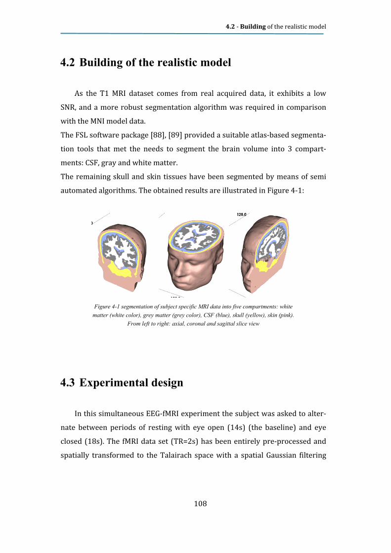
4.2 - Building of the realistic model
108
4.2 Building of the realistic model
As the T1 MRI dataset comes from real acquired data, it exhibits a low
SNR, and a more robust segmentation algorithm was required in comparison
with the MNI model data.
The FSL software package [88], [89] provided a suitable atlas-based segmenta-
tion tools that met the needs to segment the brain volume into 3 compart-
ments: CSF, gray and white matter. The remaining skull and skin tissues have been segmented by means of semi automated algorithms. The obtained results are illustrated in Figure 4-1:
4.3 Experimental design
In this simultaneous EEG-fMRI experiment the subject was asked to alter-
nate between periods of resting with eye open (14s) (the baseline) and eye
closed (18s). The fMRI data set (TR=2s) has been entirely pre-processed and
spatially transformed to the Talairach space with a spatial Gaussian filtering
Figure 4-1 segmentation of subject specific MRI data into five compartments: white
matter (white color), grey matter (grey color), CSF (blue), skull (yellow), skin (pink).
From left to right: axial, coronal and sagittal slice view

4.4 - fMRI activation imaging
109
FWHM 6mm wide. Furthermore, a head mesh and a cortical surface mesh (see
Figure 4-2 ) have been made available and reconstructed in the Talairach
space. The channels acquired are incorporated in a 62 channels cap (see Figure
4-2 ), and have been acquired at a sampling rate Fs=250Hz.
4.4 fMRI activation imaging
We ran one single study GLM on the functional data, thus obtaining both
the volumetric and cortical maps. The functional volume time course data has
been previously filtered by a spatial Gaussian kernel 6mm wide, in order to
prevent noise effects. A default predictor was used for the closed-eyes condi-
tion, showed in the figure below:
Figure 4-3 GLM standard predictor, resulting from convolution between box-car function and HRF
Figure 4-2 Left: cortical mesh source space. Right: electrodes set

4.4 - fMRI activation imaging
110
Figure 4-4 Volume map of the statistical contrast between the two conditions.
Figure 4-5. The fMRI signal timecourse averaged between points belonging to the region of interest (ROI) We built the GLM for both the experimental conditions (eyes closed and eyes open, see Figure 4-3), then a contrast map was computed, in which we com-

4.4 - fMRI activation imaging
111
pared the differences in the statistical values of each condition (Figure 4-4). Since the difference has been defined as “eyes open vs. eyes closed”, the green regions in the visual cortex mean that that region is significantly active during “eyes closed” condition, compared to “eyes open” condition. In Figure 4-5 the fMRI signal time course averaged between points belonging to the region of interest (ROI) is reported. The selected ROI belongs to the V1, and it has been projected onto the cortical surface (see Figure 4-6), to be the computational domain for the statistical analysis.
Figure 4-6 patch of interest of the cortical mesh Projecting the statistical volume map onto the cortical mesh produced the cor-tical map reported in Figure 4-7.
Figure 4-7 fMRI statistical contrast map projection on the cortical mesh

4.5 - EEG distributed source analysis
112
4.5 EEG distributed source analysis
Since the entire procedure, described in this paragraph, takes as input a
previously calculated lead field matrix, it is possible to compare the source im-
aging results among different modelling techniques. In our investigation we
used realistic (FDM) and spherical models lead fields, pre-computed using the
algorithms described in chapter 2.
4.5.1 Channel pre-processing
The EEG signal projection from the channel to the source space requires
that channel data are preliminary organized as single-trial channel data (STD) or
time-frequency data (TFD) [102], [85].
This means that, with or without final averaging and time-frequency transfor-
mation, single trials have to be extracted from continuous channel data (CTC).
Moreover, the experimental condition has to be specified.
The most important triggers we are seeking in the EEG data are called “R1”
and “S2” in the acquisition protocol, and they correspond to the fMRI trigger at
each TR and the instruction for closing eyes, respectively. We started with ana-
lyzing the data with respect to trigger “S2” by selecting a pre-trigger interval of
5000ms and a post-trigger interval of 20000ms
In order to produce time-frequency transform (which is based on the
Short-Time Fourier Transform), we set a time resolution of the analysis of
200ms, and a time window 2s wide. Since we are interested in alpha band (i.e.
around 10 Hz) signals, we filtered the EEG data up to 20Hz. A plot of the TFD gives a scaled image trial averaged positive and negative changes of the spectral power around the condition trigger. In many channels, a strong positive change in the event-related spectral perturbation (synchro-nization) induced by the status change from eye open to eye closed can be ob-served inside the alpha band (8-13 Hz).

4.5 - EEG distributed source analysis
113
In order to define the cortical region of maximal synchronization, we have
to estimate a distributed inverse solution that we will later use for projecting
EEG signals in a pre-specified time-frequency box from the channel to the
source space.
4.5.2 Covariance calculation
Recalling section 2.2.4, we now need to estimate the data covariance ma-
trix. In order to create a condition-independent inverse solution with maximal
statistical power, the STD created from all conditions in the protocol is used. In
the context of beamforming techniques the covariance matrix will be later used
to quantify the amount of interference between all possible sources “visible” in
the channel space.
4.5.3 Inverse Modeling
Now we can combine the covariance data with the previously computed
lead fields, to produce the EEG inverse problem solution. The inverse methods adopted at this point are the LCMV beamforming, which has been mentioned in chapter 2.2.4, as it has been recently shown to achieve the best results when applied to distributed source localization [20], [103]; furthermore, the well know and used WMN filter with noise based regulariza-tion (see 2.2.4.4) has also been used for comparative purpose. 4.5.4 Source time-course reconstruction
The newly computed inverse solution can be used for reconstructing the
source time-course at each point of the cortex mesh, in term of RMS power
signal (virtual electrode) [102], [85]. We reconstruct the source power time-
courses in a mesh time-course after filtering the single-trial data set.

4.5 - EEG distributed source analysis
114
For the present application, it is not interesting to project full-band or aver-aged data, but rather narrow-band time-courses, which can be obtained by us-ing continuous-wavelet-transform filters with wavelet functions adapted to the desired centre frequency and the desired duration-bandwidth ratio. A cen-tre frequency of 11 Hz and a wavelet ratio of 11 are used. It is important to check the approximate duration and bandwidth of the
wavelet for these settings before proceeding with the filtering. Provided that
the bandwidth is acceptable, the duration of the wavelet also affects the choice
of a possible decimation of the projected time courses. Here we use a decima-
tion factor of 100 which entails to resample the source power time-courses
from the original sampling period of 4 ms to a sampling period of 400ms. Since
we are interested in appreciating any induced sustained perturbation in a long
period of 20s, rather than fast transient effects, the new sampling period can
be accepted. Later, the created mesh time-course with the average induced
source power perturbations will be displayed, after the final source analysis.
4.5.5 Source imaging and statistical analysis
The approach presented in [102], [85] allows generating (series of) brain
activity maps for specific time (or time-frequency) intervals of interest and
producing source time and time-frequency plots from regions of interest pre-
specified as patches of interest (POIs). The input data of this final stage is again the TFD computed by the pre-processing step. The “target” time-frequency box will consist of the entire pe-riod of closed-eye (18s) and of the entire alpha band (8:13Hz). The baseline for the source statistical image is the entire prestimulus interval (-5000ms:0). The output of the source image analysis will be a t-map expressing the sta-
tistical significance of the target vs baseline effects in the specified time-
frequency box. For illustrative purposes it will be used a reference threshold of
t=3.50 (p=0.000486) that highlights a distributed region in the occipital cortex

4.6 - EEG-fMRI distributed Source Coupling Analysis
115
where the studied effects is relatively stronger (see Figure 4-8). Moreover, the
patch-of-interest of the “activated” region allows displaying the spatially aver-
aged source power change. The image shows the region where alpha modula-
tion was maximally expressed, compared to the rest of the cortex.
As a rule of thumb, the threshold statistical test values are typically visual-
ized using a red-to-yellow colour range for positive values and a green-to-blue
range for negative values. With this colour bar, a positive (negative) t value
just passing over a specified threshold would be coloured in red (green), while
a very highly positive (negative) t value would be coloured in yellow (blue).
4.6 EEG-fMRI distributed Source Coupling Analy-
sis
According to the considerations in paragraph 2.4.5.3, this experimental
design is suitable for being studied by means of EEG-fMRI coupling analysis.
Figure 4-8 Example of typical source imaging (cortical map on top)
and time reconstruction(plot on bottom) result

4.7 - fMRI weighting of an EEG inverse solution
116
4.6.1 Channel pre-processing
This time we selected the protocol condition that includes all fMRI trig-
gers, i.e. “R1”, and set the pre-trigger and post-trigger timings to -500.00 and
1500 ms, respectively. The data pre-processing has been ran setting a finer
time resolution for the time-frequency analysis: 20ms and a time window of
0.2s. The maximum frequency has been kept at 20 Hz.
4.6.2 Single design matrix
The next processing steps remain almost the same as in section 4.4, except
for the statistical source analysis, which now is required to output the so-
called single design matrix (SDM). According to section 2.4.5.2, we will give as
input, in the GLM analysis, a prediction of the temporal fMRI signal, basing on
the convolution of HRF with the EEG signal. The estimation of the SDM implies
collecting the EEG data series (for the condition R1) from all the trials avail-
able and, finally, z-standardized. This process requires the a-priori knowledge
of three fMRI parameters for the correct synchronization between EEG and
fMRI time points and the application of the hemodynamic correction: the time
in milliseconds of the first fMRI trigger corresponding to the first fMRI scan ac-
tually included in the analysis (in our case 0), the fMRI repetition time (TR=2)
and the number of scans constituting the fMRI time-series (this case 158).
4.7 fMRI weighting of an EEG inverse solution
The last approach we applied is conceptually the opposite of the latter,
since we first process the functional data, and then we use the informations as
a weighting for the EEG inverse solution. The fMRI processing gave an F-map

4.8 - Results
117
summarizing the fMRI main effects of interest and a second map with the per-
centage of signal change of these effects (see Figure 4-9 ).
Figure 4-9 FMRI maps used for MEG spatial weighting. F-map (left) and % s.c. map (right) for the main
effects of the conditions (linear contrast: +1, +1).
Here it is also important to apply a reasonable statistical threshold to the
F-map for discriminating sources with significant fMRI effects from sources
with non-significant main effects.
4.8 Results
4.8.1 EEG-source analysis
Figure 7-11 shows the t-maps among different forward and inverse mod-
elling techniques: realistic FDM model (see paragraph 4.2) and four-shells sen-
sor-fitted spherical model; while beamforming and WMN where used as in-
verse algorithms. The EEG source localization of these effects entailed with
finding the local peaks of the cortical maps [104] and accepting as EEG sources
the local peaks whose corresponding p-value was below 0.001 (uncorrected).
4.9 - Evaluation of brain source reconstruction capabilities
118
Moreover, the induced RMS source power perturbation time course is plotted
at bottom of each map, showing the values spatially averaged across the POI,
and temporally averaged across trials.
4.8.2 EEG-fMRI coupling
Considering the same four cases aforementioned, we illustrate in Figure 7-
12 the different fMRI predictors estimated from the EEG data, given different
inverse solutions for different modelling techniques. Furthermore, the cortical maps of the standardized t-maps are shown in Fig-ure 7-13. The p-value threshold is set to 0.00165. Figure 7-13a refers to the fMRI classic analysis, i.e. not driven by EEG data. 4.8.3 fMRI weighting of EEG inverse solution
Since the weighting of an inverse solution applies only to imaging ap-
proaches, this technique has not been used in conjunction with beamforming.
The figures report the t-maps for the realistic as well as the spherical model,
both processed by means of WMN noise normalized inverse method with fMRI
weighting and Bonferroni corrected (p=0.05).
4.9 Evaluation of brain source reconstruction capa-
bilities
This study focused on the alpha band modulation effects during an ex-
perimental “eyes open-eyes closed” protocol in an EEG-fMRI contemporary ac-
quisition. In the EEG framework, we epoched the EEG single trial data, and ex-
tracted the time-frequency components of interest (frequency band from 8 to

4.9 - Evaluation of brain source reconstruction capabilities
119
13 Hz, consistent with findings in [105]). Then the preprocessed data, as well
as the channels covariance estimation and the precomputed lead fields, en-
tered the inverse modelling algorithm to produce the source imaging and RMS
power time-course. An fMRI statistical activation map was separately computed, using a standard GLM with two different predictors for the two conditions. Then two kind of multimodal integration have been performed. First, the source power time-series were exploited to derive a predictor with source-specific information in the GLM analysis of the functional MRI. The maps illustrated in Figure 7-11a,b show that the EEG source analysis
is strongly affected by the choice of the forward modelling applied, as pointed
out also in [6, 63, 94, 106]. Even if both realistic and approximated geometry
models lead to an inverse solution centred in the visual cortex, according find-
ings in [107], they also spot different regions, sparse around the patch-of-
interest (POI) of Figure 4-6. Since the FDM algorithm applied [8] takes into ac-
count the realistic geometry of the whole head, it is reasonable to consider it
more reliable. This is true as long as the noise is mostly correlated noise,
rather than Gaussian [63]. In order to give more strongly evidences on the absolute increasing in accu-racy led by the introduction of a realistic model, a group study on a wider number of subjects will be used in required for further investigations. The first methodological consideration is focused on the choice of the in-
verse problem algorithm applied. While LORETA solution is analogous to the
noise-normalized WMN solution used in others recent works (see e.g. [85]), it
only differs from the latter by the smoothness constrain, which is embodied in
matrix R in equation ( 2 . 3 8 ), and by the requirement of a regular-grid sources
domain [69]. Here we did not use LORETA because in current literature, to our
knowledge, there are no evidences of its application in a mesh-based distrib-
uted source modelling.

4.9 - Evaluation of brain source reconstruction capabilities
120
As expected, the EEG source analysis, as well as the source temporal re-
construction, is sensitive to the inverse algorithm used. As shown in Figure
7-11c,d the beamforming technique seems to produce an inaccurate source lo-
calization when applied to the spherical forward model, thus exhibiting a low
average power time course, compared to the realistic case. However, since
beamforming has been proven to be effective in source localization and par-
ticularly in rejecting interferences in EEG signals [108], a deeper comparative
investigation of the performances of the two implementations is required.
Another methodological issue regards the regularization parameter in the
WMN spatial filtering estimation (eq. ( 2 . 4 2 )). It has been observed that, at
constant SNR guess and with the same depth factor (γ in equation ( 2 . 3 7 ), the
lambda parameter sensibly increases when computed on a realistic leadfield
matrix, compared to the spherical LF. Although in many evoked response ex-
periments [81] the used value is 5, this might not be suited for a realistic-
derived forward field, for which can be empirically verified that: trace(LLLLFDMFDMFDMFDM*L*L*L*LTTTTFDMFDMFDMFDM) ) ) ) << trace(LLLLSPHSPHSPHSPH*L*L*L*LTTTTSPHSPHSPHSPH)))) This aspect should be object of further studies. As shown in Figure 7-13, the contribute of the EEG inverse analysis to the
fMRI source localization is relevant, as already showed in [85] [102], as it
helps isolating the alpha-band effective sources of the V1 region. A closer look,
also to Figure 7-12, suggests this EEG-fMRI coupling technique does not show
to be sensitive to the forward-modelling approach used, but rather to the in-
verse modelling algorithm. In this case the beamforming seemed to perform
better than WMN, since the latter tends not to lose the left V1 activated region
(see Figure 7-13).
fMRI weighting of the EEG inverse analysis (see Figure 7-14) produces
relevant effects on source localization, confirming the findings in [74]. In spite
of EEG fMRI coupling approach, this technique is sensitive to the model
adopted, other than the fMRI weighting parameter k defined in 2.4.1.

4.9 - Evaluation of brain source reconstruction capabilities
121
As it has been observed, the regularization parameter λ increases almost li-nearly, keeping the SNR guess constant, with k . The overall effect of the func-tional constraints is to then to “smoothly bias” the EEG solution towards the most statistically significant BOLD signal changes. In the results illustrated in Figure 7-14, only two values of k have been used: 20 and 80. Other trials in-volved either smaller or greater values, but they led to totally ignoring fMRI contribution, or ignoring EEG contribution, respectively. Finally, as we expected, both the realistic and spherical models benefit from the approach.
4.9 - Evaluation of brain source reconstruction capabilities
122
5 Conclusions
In this chapter a general conclusion is given of this dissertation, followed
by brief overview of the future works.
In the first part of the research we compared different spherical and real-
istic head modelling techniques in estimating EEG forward solutions from cur-
rent dipole sources distributed on a standard cortical space reconstructed
from Montreal Neurological Institute (MNI) MRI data. Computer simulations
are presented for three different four-shell head models, two with realistic ge-
ometry, either surface-based (BEM) or volume-based (FDM), and the corre-
sponding sensor-fitted spherical-shaped model. Point Spread Function (PSF)
and Lead Field (LF) cross-correlation analyses were performed for 26 sym-
metric dipole sources to quantitatively assess models’ accuracy in EEG source
reconstruction. The results obtained demonstrate that realistic geometry can provide a factor of improvement which is particularly important when considering sources placed in the temporal or in the occipital cortex. In these situations, using a realistic head model will allow a better spatial discrimination of neural sources in comparison with the spherical model, as it can be appreciated by the analy-sis of the PSF maps as shown in chapter 3. Hence, in this investigation we have demonstrated that a significant improvement in source modelling accuracy can be obtained without significant increase in effort, namely replacing the standard spherical head model with a standardized realistically shaped FDM head model. By appropriately warping the electrode array of an individual pa-tient to the standardized model, the same realistic head model can be used for any patient with great gain in computational speed because the time-consuming numerical calculations of the FDM matrixes have already been per-formed. At the speed of modern PCs, the additional computation effort needed

4.9 - Evaluation of brain source reconstruction capabilities
123
to use this standardized model is reasonable. This is particularly true when considering the improved accuracy afforded by such a standardized FDM model and the amount of effort required to set up an individualized head mod-el. It is also worth stressing that the results presented in this dissertation, thanks to the adoption of the MNI-based models, based on a large series of MRI scans on normal controls and thus reflecting average neuroanatomy more rep-resentative of the population, can be an enrichment with respect to other stu-dies for the possibility of gathering more general information also extensible to others application studies in this field Later we increased the complexity of the MNI-based realistic model, im-
plementing a multi-subject DTI data integration that led to an accurate anisot-
ropy description of the white matter and skull bones tissues. We have also
shown a novel comparative analysis performed between isotropic and anisot-
ropic forward fields, whose results comply with previous literature’s findings.
In the last part of our studies, two methods of EEG-fMRI data integration
have been included in the multimodal framework and applied to different
modeling techniques. The preliminary results point out an improvement in
EEG source imaging reliability by means of the beamforming EEG inverse
modelling approach on a realistic forward model. Noticeably, it has been
shown that both EEG-driven fMRI, as well as fMRI-driven EEG analysis can fur-
ther improve both fMRI’s source localization and EEG’s source reconstruction
accuracy.
However, it should be considered that since in the literature there are no
group-analysis experimental studies performed with realistic modelling ap-
proach, this aspect should be further investigated. Other than this, there are
some more issues that still need to be addressed in future works: how the LF
matrix conditioning is related to the regularization parameter involved in the
source imaging approaches, and how to define an optimal pre-regularization of
the LF matrix. Furthermore the application of LAURA or LORETA inverse algo-

4.9 - Evaluation of brain source reconstruction capabilities
124
rithms, to the multimodal integration is also attractive, but requires the defini-
tion of a different source-seeking spatial domain.

4.9 - Evaluation of brain source reconstruction capabilities
125
6 Bibliography
1. Vatta, F., P. Bruno, and P. Inchingolo, Improving lesion conductivity estimate by
means of EEG source localization sensitivity to model parameter. J Clin
Neurophysiol, 2002. 19(1): p. 1-15.
2. Ebersole, J.S. and S. Hawes-Ebersole, Clinical application of dipole models in the
localization of epileptiform activity. J Clin Neurophysiol, 2007. 24(2): p. 120-9.
3. Goldman, R.I., et al., Acquiring simultaneous EEG and functional MRI. Clin
Neurophysiol, 2000. 111(11): p. 1974-80.
4. Lemieux, L., et al., Event-related fMRI with simultaneous and continuous EEG:
description of the method and initial case report. Neuroimage, 2001. 14(3): p. 780-
7.
5. Gholipour, T., et al., Reproducibility of interictal EEG-fMRI results in patients
with epilepsy. Epilepsia, 2010.
6. Meneghini, F., et al., Comparison between realistic and spherical approaches in
EEG forward modelling. Biomed Tech (Berl), 2010. 55(3): p. 133-46.
7. Vatta, F., et al., Realistic and spherical head modeling for EEG forward problem
solution: a comparative cortex-based analysis. Comput Intell Neurosci, 2010: p.
972060.
8. Meneghini, F., et al., Threedimensional eeg source reconstruction on high
performance computers methodological and computational issues. Biomed Sci
Instrum, 2008. 44: p. 336-41.
9. Vatta, F., et al., Head modeling for realistic electrical brain activity mapping
identification of a multimodal neuroimaging protocol. Biomed Sci Instrum, 2008.
44: p. 342-8.
10. Basser, P.J., J. Mattiello, and D. LeBihan, Estimation of the effective self-diffusion
tensor from the 7MR spin echo. J Magn Reson B, 1994. 103(3): p. 247-54.
11. Basser, P.J., J. Mattiello, and D. LeBihan, MR diffusion tensor spectroscopy and
imaging. Biophys J, 1994. 66(1): p. 259-67.
12. Hasan, K.M., D.L. Parker, and A.L. Alexander, Comparison of gradient encoding
schemes for diffusion-tensor MRI. J Magn Reson Imaging, 2001. 13(5): p. 769-80.
13. Koay, C.G., et al., A unifying theoretical and algorithmic framework for least
squares methods of estimation in diffusion tensor imaging. J Magn Reson, 2006.
182(1): p. 115-25.
14. Alexander, A.L., et al., A geometric analysis of diffusion tensor measurements of
the human brain. Magn Reson Med, 2000. 44(2): p. 283-91.
15. Westin, C.F., et al., Processing and visualization for diffusion tensor MRI. Med
Image Anal, 2002. 6(2): p. 93-108.
16. Makris, N., et al., Morphometry of in vivo human white matter association
pathways with diffusion-weighted magnetic resonance imaging. Ann Neurol, 1997.
42(6): p. 951-62.
17. Pajevic, S. and C. Pierpaoli, Color schemes to represent the orientation of
anisotropic tissues from diffusion tensor data: application to white matter fiber
tract mapping in the human brain. Magn Reson Med, 1999. 42(3): p. 526-40.

4.9 - Evaluation of brain source reconstruction capabilities
126
18. Witwer, B.P., et al., Diffusion-tensor imaging of white matter tracts in patients
with cerebral neoplasm. J Neurosurg, 2002. 97(3): p. 568-75.
19. Lazar, M., et al., White matter reorganization after surgical resection of brain
tumors and vascular malformations. AJNR Am J Neuroradiol, 2006. 27(6): p.
1258-71.
20. Grech, R., et al., Review on solving the inverse problem in EEG source analysis. J
Neuroeng Rehabil, 2008. 5: p. 25.
21. He, B., D. Yao, and J. Lian, High-resolution EEG: on the cortical equivalent
dipole layer imaging. Clin Neurophysiol, 2002. 113(2): p. 227-35.
22. Hara, J., T. Musha, and W.R. Shankle, Approximating dipoles from human EEG
activity: the effect of dipole source configuration on dipolarity using single dipole
models. IEEE Trans Biomed Eng, 1999. 46(2): p. 125-9.
23. Zhou, H. and A. van Oosterom, Computation of the potential distribution in a four-
layer anisotropic concentric spherical volume conductor. IEEE Trans Biomed
Eng, 1992. 39(2): p. 154-8.
24. Klepfer, R.N., C.R. Johnson, and R.S. Macleod, The effects of inhomogeneities and
anisotropies on electrocardiographic fields: a 3-D finite-element study. IEEE
Trans Biomed Eng, 1997. 44(8): p. 706-19.
25. Marin, G., et al., Influence of skull anisotropy for the forward and inverse problem
in EEG: simulation studies using FEM on realistic head models. Hum Brain Mapp,
1998. 6(4): p. 250-69.
26. Akhtari, M., et al., A model for frequency dependence of conductivities of the live
human skull. Brain Topogr, 2003. 16(1): p. 39-55.
27. Nicholson, P.W., Specific impedance of cerebral white matter. Exp Neurol, 1965.
13(4): p. 386-401.
28. Le Bihan, D., et al., Diffusion tensor imaging: concepts and applications. J Magn
Reson Imaging, 2001. 13(4): p. 534-46.
29. Tuch, D.S., Q-ball imaging. Magn Reson Med, 2004. 52(6): p. 1358-72.
30. Bastiani, M., Fibre-tracking in high angular resolution diffusion imaging of
cortical white matter: crossing-fibre models, graph tractography and cortico-
cortical connectome tractography in Department of Cognitive 7euroscience,
Faculty of Psychology and Cognitive 7euroscience
2009, Maastricht University.
31. Plonsey, R. and D.B. Heppner, Considerations of quasi-stationarity in
electrophysiological systems. Bull Math Biophys, 1967. 29(4): p. 657-64.
32. Mosher, J.C., R.M. Leahy, and P.S. Lewis, EEG and MEG: forward solutions for
inverse methods. IEEE Trans Biomed Eng, 1999. 46(3): p. 245-59.
33. Vanrumste, B., et al., The validation of the finite difference method and reciprocity
for solving the inverse problem in EEG dipole source analysis. Brain Topogr,
2001. 14(2): p. 83-92.
34. Weinstein, D., L. Zhukov, and C. Johnson, Lead-field bases for
electroencephalography source imaging. Ann Biomed Eng, 2000. 28(9): p. 1059-
65.
35. Zhang, Z., A fast method to compute surface potentials generated by dipoles within
multilayer anisotropic spheres. Phys Med Biol, 1995. 40(3): p. 335-49.
36. Cuffin, B.N., Effects of head shape on EEG's and MEG's. IEEE Trans Biomed
Eng, 1990. 37(1): p. 44-52.
37. Cuffin, B.N., Eccentric spheres models of the head. IEEE Trans Biomed Eng,
1991. 38(9): p. 871-8.

4.9 - Evaluation of brain source reconstruction capabilities
127
38. Huang, M.X., J.C. Mosher, and R.M. Leahy, A sensor-weighted overlapping-
sphere head model and exhaustive head model comparison for MEG. Phys Med
Biol, 1999. 44(2): p. 423-40.
39. Vatta, F., P. Bruno, and P. Inchingolo, Multiregion bicentric-spheres models of the
head for the simulation of bioelectric phenomena. IEEE Trans Biomed Eng, 2005.
52(3): p. 384-9.
40. Gutierrez, D. and A. Nehorai, Array response kernels for EEG and MEG in
multilayer ellipsoidal geometry. IEEE Trans Biomed Eng, 2008. 55(3): p. 1103-11.
41. Ermer, J.J., et al., Rapidly recomputable EEG forward models for realistic head
shapes. Phys Med Biol, 2001. 46(4): p. 1265-81.
42. Fuchs, M., et al., An improved boundary element method for realistic volume-
conductor modeling. IEEE Trans Biomed Eng, 1998. 45(8): p. 980-97.
43. Zhang, Y., et al., A cortical potential imaging study from simultaneous extra- and
intracranial electrical recordings by means of the finite element method.
Neuroimage, 2006. 31(4): p. 1513-24.
44. Hallez, H., et al., Review on solving the forward problem in EEG source analysis. J
Neuroeng Rehabil, 2007. 4: p. 46.
45. Fuchs, M., M. Wagner, and J. Kastner, Boundary element method volume
conductor models for EEG source reconstruction. Clin Neurophysiol, 2001.
112(8): p. 1400-7.
46. Ramon, C., J. Haueisen, and P.H. Schimpf, Influence of head models on
neuromagnetic fields and inverse source localizations. Biomed Eng Online, 2006.
5: p. 55.
47. Yvert, B., et al., A systematic evaluation of the spherical model accuracy in EEG
dipole localization. Electroencephalogr Clin Neurophysiol, 1997. 102(5): p. 452-9.
48. Cuffin, B.N., Effects of local variations in skull and scalp thickness on EEG's and
MEG's. IEEE Trans Biomed Eng, 1993. 40(1): p. 42-8.
49. Brody, D.A., F.H. Terry, and R.E. Ideker, Eccentric dipole in a spherical medium:
generalized expression for surface potentials. IEEE Trans Biomed Eng, 1973.
20(2): p. 141-3.
50. Cuffin, B.N. and D. Cohen, Comparison of the magnetoencephalogram and
electroencephalogram. Electroencephalogr Clin Neurophysiol, 1979. 47(2): p.
132-46.
51. Ary, J.P., S.A. Klein, and D.H. Fender, Location of sources of evoked scalp
potentials: corrections for skull and scalp thicknesses. IEEE Trans Biomed Eng,
1981. 28(6): p. 447-52.
52. Berg, P. and M. Scherg, A fast method for forward computation of multiple-shell
spherical head models. Electroencephalogr Clin Neurophysiol, 1994. 90(1): p. 58-
64.
53. Sarvas, J., Basic mathematical and electromagnetic concepts of the biomagnetic
inverse problem. Phys Med Biol, 1987. 32(1): p. 11-22.
54. de Munck, J.C., A linear discretization of the volume conductor boundary integral
equation using analytically integrated elements. IEEE Trans Biomed Eng, 1992.
39(9): p. 986-90.
55. Oostendorp, T.F. and A. van Oosterom, Source parameter estimation in
inhomogeneous volume conductors of arbitrary shape. IEEE Trans Biomed Eng,
1989. 36(3): p. 382-91.

4.9 - Evaluation of brain source reconstruction capabilities
128
56. Ferguson, A.S., X. Zhang, and G. Stroink, A complete linear discretization for
calculating the magnetic field using the boundary element method. IEEE Trans
Biomed Eng, 1994. 41(5): p. 455-60.
57. George, J.S., et al., Mapping function in the human brain with
magnetoencephalography, anatomical magnetic resonance imaging, and
functional magnetic resonance imaging. J Clin Neurophysiol, 1995. 12(5): p. 406-
31.
58. Yvert, B., A. Crouzeix-Cheylus, and J. Pernier, Fast realistic modeling in
bioelectromagnetism using lead-field interpolation. Hum Brain Mapp, 2001. 14(1):
p. 48-63.
59. Fuchs, M., et al., A standardized boundary element method volume conductor
model. Clin Neurophysiol, 2002. 113(5): p. 702-12.
60. Bruno, P., et al., A FDM anisotropic formulation for EEG simulation. Conf Proc
IEEE Eng Med Biol Soc, 2006. 1: p. 1121-5.
61. Saleheen, H.I. and K.T. Ng, 7ew finite difference formulations for general
inhomogeneous anisotropic bioelectric problems. IEEE Trans Biomed Eng, 1997.
44(9): p. 800-9.
62. Schimpf, P.H., C. Ramon, and J. Haueisen, Dipole models for the EEG and MEG.
IEEE Trans Biomed Eng, 2002. 49(5): p. 409-18.
63. Vanrumste, B., et al., Comparison of performance of spherical and realistic head
models in dipole localization from noisy EEG. Med Eng Phys, 2002. 24(6): p. 403-
18.
64. Vanrumste, B., et al., Dipole location errors in electroencephalogram source
analysis due to volume conductor model errors. Med Biol Eng Comput, 2000.
38(5): p. 528-34.
65. Van Hoey, G., et al., Influence of measurement noise and electrode mislocalisation
on EEG dipole-source localisation. Med Biol Eng Comput, 2000. 38(3): p. 287-96.
66. de Munck, J.C., B.W. van Dijk, and H. Spekreijse, Mathematical dipoles are
adequate to describe realistic generators of human brain activity. IEEE Trans
Biomed Eng, 1988. 35(11): p. 960-6.
67. He, B. and Z. Liu, Multimodal Functional 7euroimaging: Integrating Functional
MRI and EEG/MEG. IEEE Rev Biomed Eng, 2008. 1(2008): p. 23-40.
68. Dale, A.M., et al., Dynamic statistical parametric mapping: combining fMRI and
MEG for high-resolution imaging of cortical activity. Neuron, 2000. 26(1): p. 55-
67.
69. Pascual-Marqui, R.D., Standardized low-resolution brain electromagnetic
tomography (sLORETA): technical details. Methods Find Exp Clin Pharmacol,
2002. 24 Suppl D: p. 5-12.
70. B. D. Van Veen , K.M.B., Beamforming: A versatile approach to spatial filtering.
IEEE Acoustics, Speech and Signal Processing Magazine, 1988. 5: p. 4-24.
71. Ogawa, S., et al., Brain magnetic resonance imaging with contrast dependent on
blood oxygenation. Proc Natl Acad Sci U S A, 1990. 87(24): p. 9868-72.
72. Friston, K.J., et al., Characterizing dynamic brain responses with fMRI: a
multivariate approach. Neuroimage, 1995. 2(2): p. 166-72.
73. Friston, K.J., et al., Value-dependent selection in the brain: simulation in a
synthetic neural model. Neuroscience, 1994. 59(2): p. 229-43.
74. Babiloni, F., et al., Multimodal integration of high-resolution EEG and functional
magnetic resonance imaging data: a simulation study. Neuroimage, 2003. 19(1): p.
1-15.

4.9 - Evaluation of brain source reconstruction capabilities
129
75. Liu, A.K., J.W. Belliveau, and A.M. Dale, Spatiotemporal imaging of human brain
activity using functional MRI constrained magnetoencephalography data: Monte
Carlo simulations. Proc Natl Acad Sci U S A, 1998. 95(15): p. 8945-50.
76. Magistretti, P.J. and L. Pellerin, Cellular mechanisms of brain energy metabolism
and their relevance to functional brain imaging. Philos Trans R Soc Lond B Biol
Sci, 1999. 354(1387): p. 1155-63.
77. Malonek, D. and A. Grinvald, Interactions between electrical activity and cortical
microcirculation revealed by imaging spectroscopy: implications for functional
brain mapping. Science, 1996. 272(5261): p. 551-4.
78. Puce, A., et al., Functional magnetic resonance imaging of sensory and motor
cortex: comparison with electrophysiological localization. J Neurosurg, 1995.
83(2): p. 262-70.
79. Di Russo, F., et al., Identification of the neural sources of the pattern-reversal
VEP. Neuroimage, 2005. 24(3): p. 874-86.
80. Opitz, B., et al., The functional neuroanatomy of novelty processing: integrating
ERP and fMRI results. Cereb Cortex, 1999. 9(4): p. 379-91.
81. Lin, F.H., et al., Spectral spatiotemporal imaging of cortical oscillations and
interactions in the human brain. Neuroimage, 2004. 23(2): p. 582-95.
82. Babiloni, F., et al., Estimation of the cortical functional connectivity with the
multimodal integration of high-resolution EEG and fMRI data by directed transfer
function. Neuroimage, 2005. 24(1): p. 118-31.
83. Astolfi, L., et al., Estimation of the cortical connectivity by high-resolution EEG
and structural equation modeling: simulations and application to finger tapping
data. IEEE Trans Biomed Eng, 2005. 52(5): p. 757-68.
84. P.-J. Lahaye, S.B., J.-B. Poline, and L. Garnero, Fusion of simultaneous fMRI/EEG
data based on the electro-metabolic coupling. Proc. IEEE ISBI, 2004: p. 864-867.
85. Esposito, F., C. Mulert, and R. Goebel, Combined distributed source and single-
trial EEG-fMRI modeling: application to effortful decision making processes.
Neuroimage, 2009. 47(1): p. 112-21.
86. Ramon, C., P.H. Schimpf, and J. Haueisen, Influence of head models on EEG
simulations and inverse source localizations. Biomed Eng Online, 2006. 5: p. 10.
87. Wolters, C.H., et al., Influence of tissue conductivity anisotropy on EEG/MEG field
and return current computation in a realistic head model: a simulation and
visualization study using high-resolution finite element modeling. Neuroimage,
2006. 30(3): p. 813-26.
88. Woolrich, M.W., et al., Bayesian analysis of neuroimaging data in FSL.
Neuroimage, 2009. 45(1 Suppl): p. S173-86.
89. Smith, S.M., et al., Advances in functional and structural MR image analysis and
implementation as FSL. Neuroimage, 2004. 23 Suppl 1: p. S208-19.
90. Smith, S.M., et al., Tract-based spatial statistics: voxelwise analysis of multi-
subject diffusion data. Neuroimage, 2006. 31(4): p. 1487-505.
91. Wang, Y., D.R. Haynor, and Y. Kim, An investigation of the importance of
myocardial anisotropy in finite-element modeling of the heart: methodology and
application to the estimation of defibrillation efficacy. IEEE Trans Biomed Eng,
2001. 48(12): p. 1377-89.
92. Ollikainen, J.O., et al., Effects of local skull inhomogeneities on EEG source
estimation. Med Eng Phys, 1999. 21(3): p. 143-54.
93. Rush, S. and D.A. Driscoll, Current distribution in the brain from surface
electrodes. Anesth Analg, 1968. 47(6): p. 717-23.

4.9 - Evaluation of brain source reconstruction capabilities
130
94. Huiskamp, G., et al., The need for correct realistic geometry in the inverse EEG
problem. IEEE Trans Biomed Eng, 1999. 46(11): p. 1281-7.
95. Liu, Z., F. Kecman, and B. He, Effects of fMRI-EEG mismatches in cortical
current density estimation integrating fMRI and EEG: a simulation study. Clin
Neurophysiol, 2006. 117(7): p. 1610-22.
96. Finke, S., R.M. Gulrajani, and J. Gotman, Conventional and reciprocal approaches
to the inverse dipole localization problem of electroencephalography. IEEE Trans
Biomed Eng, 2003. 50(6): p. 657-66.
97. Crevecoeur, G., et al., A hybrid algorithm for solving the EEG inverse problem
from spatio-temporal EEG data. Med Biol Eng Comput, 2008. 46(8): p. 767-77.
98. Ramon, C., P.H. Schimpf, and J. Haueisen, Effect of model complexity on EEG
source localizations. Neurol Clin Neurophysiol, 2004. 2004: p. 81.
99. Wen, P. and K. Pope, Realistic human head model for EEG from both the geometry
and conductivity aspects. Australas Phys Eng Sci Med, 2003. 26(1): p. 1-5.
100. Zou, Q., et al., Functional connectivity between the thalamus and visual cortex
under eyes closed and eyes open conditions: a resting-state fMRI study. Hum Brain
Mapp, 2009. 30(9): p. 3066-78.
101. Goebel, R., F. Esposito, and E. Formisano, Analysis of functional image analysis
contest (FIAC) data with brainvoyager QX: From single-subject to cortically
aligned group general linear model analysis and self-organizing group
independent component analysis. Hum Brain Mapp, 2006. 27(5): p. 392-401.
102. Esposito, F., et al., Distributed analysis of simultaneous EEG-fMRI time-series:
modeling and interpretation issues. Magn Reson Imaging, 2009. 27(8): p. 1120-30.
103. Chen, Y.S., et al., Maximum contrast beamformer for electromagnetic mapping of
brain activity. IEEE Trans Biomed Eng, 2006. 53(9): p. 1765-74.
104. Hauk, O., Keep it simple: a case for using classical minimum norm estimation in
the analysis of EEG and MEG data. Neuroimage, 2004. 21(4): p. 1612-21.
105. Barry, R.J., et al., EEG differences between eyes-closed and eyes-open resting
conditions. Clin Neurophysiol, 2007. 118(12): p. 2765-73.
106. Vatta, F., et al., Comparison of realistic head modeling methods in EEG source
imaging - biomed 2010. Biomed Sci Instrum, 2010. 46: p. 398-403.
107. Marx, E., et al., Eyes open and eyes closed as rest conditions: impact on brain
activation patterns. Neuroimage, 2004. 21(4): p. 1818-24.
108. Brookes, M.J., et al., Simultaneous EEG source localisation and artifact rejection
during concurrent fMRI by means of spatial filtering. Neuroimage, 2008. 40(3): p.
1090-104.

7 Figures
Figure 7-1PSF(rdm) inflated maps for dipole source n. 5, oriented along the y-axis (frontal to occipital).
Figure 7-2PSF(corr) inflated map for dipole source n. 5, oriented along the y-axis (frontal to occipital).

132
Figure 7-3FWHM values for PSF(rdm) computed over the whole cortex mesh, for the three different source orientations x, y and z, on
the first, second and third columns, respectively. The reported values have also been arranged according to the dipole positions
components x, y and z on the first, second and third rows. Black dots: realistic model. Grey dots: spherical model

133
Figure 7-4FWHM values for PSF(corr) computed over the whole cortex mesh, for the three different source orientations x, y and z, on the
first, second and third columns, respectively.The reported values have also been arranged according to the dipole positions components x, y
and z on the first, second and third rows. Black dots: realistic model. Grey dots: spherical model.

134
Figure 7-5 RMS inflated maps of the FWHM values for PSF(rdm). Realistic model (left) and spherical
model (right).
Figure 7-6 RMS inflated maps of the FWHM values for PSF(corr). Realistic model (left) and spherical model
(right).

Figure
Figure
Figure 7-7 MC maps.
map, with the electrodes, coloured according to
Figure 7-8 PSF maps obtained for source 2 placed in the temporal
in the Talairach coordinate
MC maps. (Left) Mutual correlation values between realistic and spherical LFs. (Right) The same
map, with the electrodes, coloured according to
PSF maps obtained for source 2 placed in the temporal
in the Talairach coordinate system: (a) sensor
(Left) Mutual correlation values between realistic and spherical LFs. (Right) The same
map, with the electrodes, coloured according to
PSF maps obtained for source 2 placed in the temporal
system: (a) sensor
135
(Left) Mutual correlation values between realistic and spherical LFs. (Right) The same
map, with the electrodes, coloured according to
PSF maps obtained for source 2 placed in the temporal
system: (a) sensor-fitted spherical model; (b) BEM model; (c)
model.
(Left) Mutual correlation values between realistic and spherical LFs. (Right) The same
map, with the electrodes, coloured according to mutual correlation values.
PSF maps obtained for source 2 placed in the temporal region, for the
fitted spherical model; (b) BEM model; (c)
(Left) Mutual correlation values between realistic and spherical LFs. (Right) The same
rrelation values.
region, for the x-oriented source,
fitted spherical model; (b) BEM model; (c)
(Left) Mutual correlation values between realistic and spherical LFs. (Right) The same
oriented source,
fitted spherical model; (b) BEM model; (c) FDM
(Left) Mutual correlation values between realistic and spherical LFs. (Right) The same

136
Figure 7-9 Differences between the FWHM values of the RMS PSF maps for the three couples of analyzed head
models, computed as the difference between values of FWHMModel1 and FWHMModel2 over the cortex mesh
(FWHMModel1 − FWHMModel2). (A, B) FWHMBEM − FWHMFDM; (C, D) FWHMSPH −FWHMBEM; (E, F) FWHMSPH
−FWHMFDM. Positive values in the computed FWHMModel1 −FWHMModel2 differences are represented in red;
negative values are represented in blue. Red zones correspond to a smaller spatial extent and hence to abetter
capacity in terms of spatial discrimination of neural sources of Model 2 with respect to Model 1 for the different
model pairs.
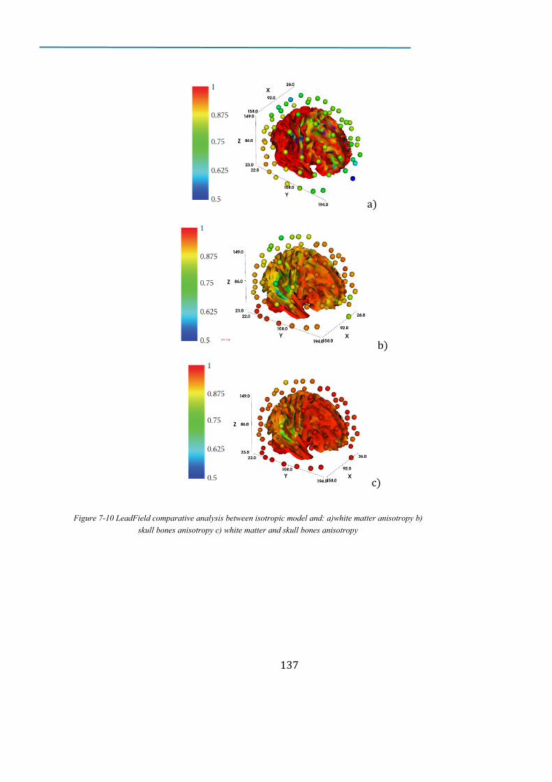
137
a)
b)
c)
Figure 7-10 LeadField comparative analysis between isotropic model and: a)white matter anisotropy b)
skull bones anisotropy c) white matter and skull bones anisotropy

138
b) a)

139
Figure 7-11 EEG source imaging results: a) model: spherical, inverse: WM7. b)model: FDM, inverse: WM7. c)
model:spherical, inverse: beamforming. d) model: realistic FDMl, inverse:beamforming c) d)
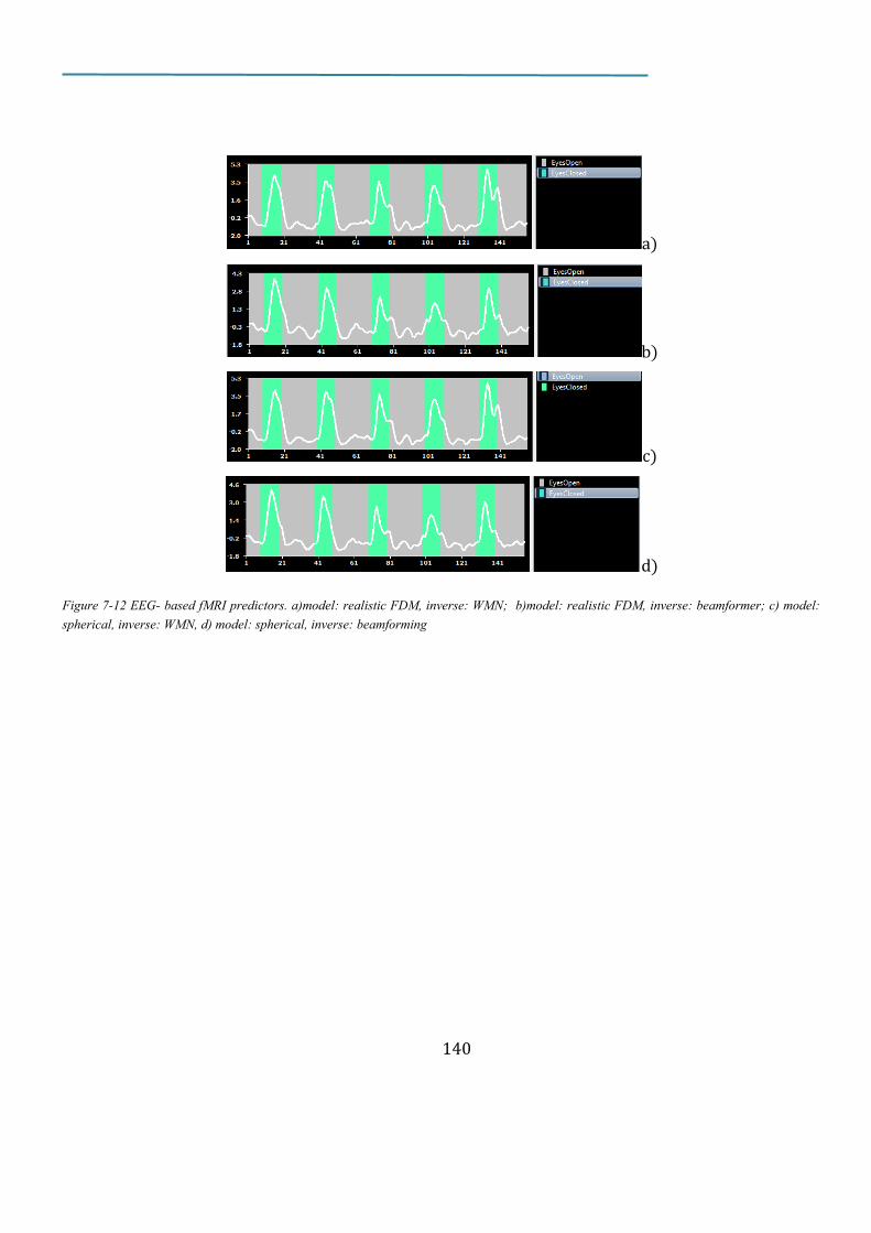
140
a)
b)
c)
d) Figure 7-12 EEG- based fMRI predictors. a)model: realistic FDM, inverse: WM7; b)model: realistic FDM, inverse: beamformer; c) model:
spherical, inverse: WM7, d) model: spherical, inverse: beamforming

141
a)
b) c)
d) e) Figure 7-13 Statistical t-maps.resulting from EEG-fMRI coupling a) fMRI-only GLM analysis. b)model: realistic FDM, inverse: WM7;
c)model: realistic FDM, inverse: beamformer; d) model: spherical, inverse: WM7, e) model: spherical, inverse: beamforming

142
a) b)

143
c) d) Figure 7-14 t-maps resulting from EEG source analysis with fMRI weighting. a) realistic (FDM) model with fMRI weighting 20. b) realistic
(FDM) model with fMRI weighting 80. c) spherical model with fMRI weighting 20. d) spherical model with weighting 80.


8
Ta
ble
s
Ta
ble
8-1
PSF
(rd
m)p
ara
met
ers

14
6
T
ab
le 8
-2P
SF
(co
rr)
pa
ram
eter
s
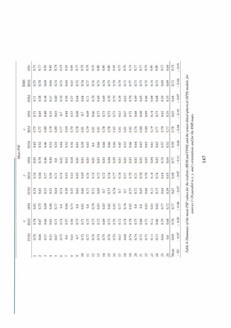
14
7
Ta
ble
8-3
Su
mm
ary
of
the
mea
n P
SF
valu
es f
or
the
reali
stic
(B
EM
an
d F
DM
) a
nd
th
e se
nso
r-fi
tted
sp
her
ical
(SP
H)
mo
del
s, f
or
sou
rces
1÷
26
pa
rall
el t
o x
, y,
and
z o
rien
tati
ons
an
d f
or
the
RM
S m
ap
s.

14
8
Ta
ble
8-4
Su
mm
ary
of
the
min
imum
PSF
va
lues
for
the
reali
stic
(B
EM
an
d F
DM
) a
nd
th
e se
nso
r-fi
tted
sp
her
ical
(SP
H)
mo
del
s, f
or
sou
rces
1÷
26
pa
rall
el t
o x
, y
an
d z
ori
enta
tio
ns
and
fo
r th
e R
MS
map
s.

14
9
Ta
ble
8-5
Su
mm
ary
of
the
FW
HM
PSF
valu
es f
or
the
reali
stic
(B
EM
an
d F
DM
) a
nd
th
e se
nso
r-fi
tted
sp
her
ical
(SP
H)
mo
del
s,
for
sou
rces
1÷
26
pa
rall
el t
o x
, y
an
d z
ori
enta
tions
an
d f
or
the
RM
S m
ap
s.