multilevel sem strategies for evaluating mediation in ... in social science research, ... analysis...

Multivariate Behavioral Research, 46:691–731, 2011

Copyright © Taylor & Francis Group, LLC

ISSN: 0027-3171 print/1532-7906 online

DOI: 10.1080/00273171.2011.589280

2009 Cattell Award Address Paper

Multilevel SEM Strategies forEvaluating Mediation in

Three-Level Data

Kristopher J. PreacherUniversity of Kansas

Strategies for modeling mediation effects in multilevel data have proliferated over

the past decade, keeping pace with the demands of applied research. Approaches

for testing mediation hypotheses with 2-level clustered data were first proposed

using multilevel modeling (MLM) and subsequently using multilevel structural

equation modeling (MSEM) to overcome several limitations of MLM. Because 3-

level clustered data are becoming increasingly common, it is necessary to develop

methods to assess mediation in such data. Whereas MLM easily accommodates

3-level data, MSEM does not. However, it is possible to specify and estimate

some 3-level mediation models using both single- and multilevel SEM. Three

new alternative approaches are proposed for fitting 3-level mediation models using

single- and multilevel SEM, and each method is demonstrated with simulated data.

Discussion focuses on the advantages and disadvantages of these approaches as

well as directions for future research.

The analysis of indirect effects (mediation) is becoming a very useful and popular

practice in social science research, with thousands of articles using mediation

analysis published annually. In many of these studies, researchers are interested

in testing mediation hypotheses with clustered data. For example, in educational

settings students are nested within classrooms, and in longitudinal settings re-

Correspondence concerning this article should be addressed to Kristopher J. Preacher, Depart-

ment of Psychology and Human Development, Vanderbilt University, 230 Appleton Place, Peabody

#552, Nashville, TN 37203. E-mail: [email protected]

691

692 PREACHER

peated measures are nested within persons. Clustered data require modeling

techniques that account for clustering, such as multilevel modeling (MLM).

There are major advantages associated with MLM-based approaches over

single-level methods if the data are hierarchically structured. One advantage

of using MLM methods is that they model cluster-induced violations of inde-

pendence, yielding more accurate standard errors (SEs) and less biased effects.

Second, MLM permits intercepts and slopes to vary randomly across clusters.

Third, using multilevel methods can help researchers avoid committing some

classic level-of-analysis fallacies. Using single-level methods, researchers may

feel obliged to aggregate some of their variables to a higher level. Aggregation

may lead to committing the ecological fallacy in which incorrect inferences

are made about cases based on aggregate statistics. Disaggregating higher level

data to a lower level, on the other hand, may lead to the atomistic fallacy

in which incorrect inferences are made about groups based on individuals. The

consequences of committing these fallacies in three-level data are more complex

than in two-level data; for example, incorrectly omitting the middle level of

a three-level design may entail committing both the ecological and atomistic

fallacies and can bias parameters and SEs throughout the model (Moerbeek,

2004). Clearly, if the data are hierarchically clustered, a modeling strategy that

accounts for clustering should be used.

ASSESSING MEDIATION IN MULTILEVEL DATA

Strategies for modeling mediation effects in multilevel designs have proliferated

over the past decade, keeping pace with the demands of applied research.

Approaches for testing mediation with two-level data were first proposed using

MLM (Bauer, Preacher, & Gil, 2006; Kenny, Korchmaros, & Bolger, 2003;

Krull & MacKinnon, 1999, 2001; Pituch & Stapleton, 2008; Pituch, Stapleton,

& Kang, 2006; Pituch, Whittaker, & Stapleton, 2005). However, whereas the

various MLM-based approaches represent an improvement over single-level

regression-based methods, they have potentially serious limitations. First, the

effect of a Level 1 regressor on a Level 1 outcome using standard MLM

procedures is actually a conflation of two slopes: the Within (W) slope (the

effect of within-cluster individual differences in a regressor on within-cluster

individual differences in the outcome) and the Between (B) slope (the effect of

between-cluster differences in the regressor on between-cluster differences in the

outcome) (Hedeker & Gibbons, 2006; Kreft, de Leeuw, & Aiken, 1995; Lüdtke

et al., 2008; Neuhaus & Kalbfleisch, 1998; Neuhaus & McCulloch, 2006). The

conflated slope estimate is often difficult to interpret because it is a weighted

average of the B and W slopes. Although this problem can be remedied to some

extent by centering the regressor at cluster means and introducing both the

mean-centered variable and its cluster mean as regressors (MacKinnon, 2008;

MSEM FOR THREE-LEVEL MEDIATION 693

Zhang, Zyphur, & Preacher, 2009), the B effect will be biased toward the W

effect to the extent that the intraclass correlation (ICC) and cluster sizes (nj )

are small (Lüdtke et al., 2008). Second, MLM approaches cannot accommodate

dependent variables that are assessed at Level 2 or higher levels. However,

there is no shortage of theories predicting such bottom-up, micro-macro, or

emergent effects in the literature. Methods proposed to deal with this problem

do not provide complete solutions (see Preacher, Zyphur, & Zhang, 2010, for a

review). A third limitation of the MLM framework is that the researcher must

assume that the variables are free of measurement error. This problem, too, can

be corrected in a limited fashion using MLM (Chou, Bentler, & Pentz, 2000;

Raudenbush, Rowan, & Kang, 1991), but the solutions are somewhat involved

and not as flexible or general as the methods discussed subsequently.

A more inclusive and flexible multilevel structural equation modeling

(MSEM) approach for assessing mediation in two-level data was described

recently (Preacher, Zhang, & Zyphur, 2011; Preacher et al., 2010). This approach

builds on the general MSEM described by B. O. Muthén and Asparouhov (2008)

and is implemented in recent versions of Mplus (L. K. Muthén & Muthén, 1998–

2010). The MSEM method involves separation of observed variables involved

in a mediation model into latent B and W components; these components are

modeled separately but simultaneously in order to estimate relationships at each

level. This method is elaborated upon in the next section; full details are provided

by Preacher et al. (2011) and Preacher et al. (2010).

Three-level data are now common throughout the social sciences. Typi-

cal examples include repeated measures nested within children, who in turn

are nested within schools (e.g., the Early Childhood Longitudinal Study; U.S.

Department of Education, 2000), and children within families within census

tracts (e.g., the National Longitudinal Survey of Children and Youth; Statistics

Canada, 1996). Despite the broad utility and popularity of mediation modeling

and the increased availability of three-level data, little has been written on

assessing mediation in three-level data hierarchies. A notable exception is Pituch,

Murphy, and Tate (2010), who extend the traditional MLM approach to three-

level models. The MSEM framework has the potential to provide a more flexible

and comprehensive modeling approach for handling a variety of data structures

and models of varying complexity. The logic of two-level implementations

of MSEM translates straightforwardly to three levels, but to date there is no

generally available software implementation to permit researchers to apply three-

level MSEM. Some authors have extended MSEM to accommodate three-level

(e.g., Bauer, 2003; Duncan et al., 1997; B. Muthén, 1997a, 1997b; B. O. Muthén

& Asparouhov, 2011; Rabe-Hesketh, Skrondal, & Pickles, 2004; Yau, Lee, &

Poon, 1993) and even four-level data (Bovaird, 2007; Duncan, Duncan, Okut,

Strycker, & Li, 2002; Duncan, Duncan, & Strycker, 2006; B. O. Muthén &

Asparouhov, 2011). However, none of these methods is ideally suited for three-

level mediation analysis for one or more of the following reasons: (a) some of

694 PREACHER

these methods apply only to balanced data (in which all clusters are of equal

size), (b) some are not implemented in widely available software, (c) some

provide only conflated slopes, (d) some are limited to growth curve modeling,

and (e) some do not permit random slopes.

Clearly, applied researchers could benefit from the availability of a general

modeling framework that (a) can accommodate unbalanced cluster sizes, (b) can

be implemented using widely available software, (c) can estimate separate slopes

at each level if appropriate, (d) can be applied to both longitudinal and cross-

sectional multilevel data, and (e) can accommodate random slopes. MSEM

possesses all of these characteristics, so potentially MSEM is ideally suited

for modeling mediation in three-level data. Furthermore, as a generalization

of structural equation modeling (SEM), MSEM (f) provides the opportunity to

model constructs as latent variables with multiple observed indicators to reduce

the effects of measurement error and (g) enables researchers to evaluate the fit of

the model to data. The ability to incorporate latent variables and evaluate model

fit is currently limited in the traditional MLM framework. My purpose in this

article is to propose three novel approaches for applying MSEM to three-level

data for the purpose of modeling mediation effects. Each of these approaches

includes some of the desirable features listed earlier.

I first provide a brief overview of the MSEM approach for assessing medi-

ation effects in two-level data, then extend this method to accommodate three

levels of the data hierarchy. Discussion is facilitated by the provision of both

equations and path diagrams. Then, each approach is illustrated using simulated

data. Finally, the advantages and disadvantages of these alternative models are

discussed, and necessary future developments are suggested.

OVERVIEW OF AN MSEM APPROACH FOR

ASSESSING MEDIATION IN TWO-LEVEL DATA

There are many approaches to combining MLM and SEM. The specific MSEM

approach adopted in this article is that discussed by B. O. Muthén and As-

parouhov (2008, 2011); described by Heck and Thomas (2009), Hox (2010), and

Kaplan (2009); and implemented in recent versions of Mplus (L. K. Muthén &

Muthén, 1998–2010). B. O. Muthén and Asparouhov’s (2008) two-level model

involves three fundamental equations:

Measurement model: Yij D �j C ƒj ˜ij C Kj Xij C ©ij (1a)

Within structural model: ˜ij D ’j C Bj ˜ij C �j Xij C —ij (1b)

Between structural model: ˜j D � C “˜j C ”Xj C —j ; (1c)


where i and j index, respectively, cases (Level 1 units) and clusters (Level 2

units). Vectors and matrices with j subscripts contain elements that may vary

across clusters. Yij .p�1/ is a vector of measured variables; �j .p�1/ contains

intercepts; ©ij .p � 1/ is a vector of Level 1 errors (or unique factors in SEM

parlance); ƒj .p � m/ is a matrix of loadings linking observed variables to m

latent variables; ˜ij .m�1/ is a vector of latent variables or random coefficients;

Xij .q � 1/ and Xj .s � 1/ contain, respectively, exogenous Level 1 and Level 2

regressors; ’j .m � 1/ contains latent intercepts; Kj .p � q/, �j .m � q/, and

Bj .m � m/ contain structural coefficients; ˜j .r � 1/ contains all of the j -

subscripted random coefficients from �j , ƒj , Kj , ’j , Bj , and �j ; � .r � 1/

contains means of those coefficients; “ .r � r/ and ” .r � s/ contain structural

coefficients linking random effects to each other and to exogenous regressors,

respectively; and —ij .m � 1/ and —j .r � 1/ contain, respectively, residuals

for Level 1 and Level 2 latent variable and random effect regressions. Finally,

—ij � MVN.0; ‰/ and —j � MVN.0; §/.

For present purposes, the equations composing this general model may be

simplified. There are various ways to do this, all of which yield identical models.

First, without loss of generality, assume all variables are measured (not latent).

Assume no error variance at Level 1, and thus remove ©ij from the model.

Further assume the variable intercepts (in �j ) are zero and that ƒj D ƒ.

All variables may be treated as endogenous, which removes Xij and Xj from

consideration. These simplifications yield

Measurement model: Yij D ƒ˜ij (2a)

Within structural model: ˜ij D ’j C Bj ˜ij C —ij (2b)

Between structural model: ˜j D � C “˜j C —j : (2c)

Equations 2a–2c can be used to define a variety of single- and two-level

mediation models, as discussed by Preacher et al. (2010). For example, given a

1-2-1 design (in which a Level 1 independent variable Xij is thought to affect a

Level 2 mediator Mj , which in turn is thought to influence a Level 1 outcome

Yij ) and fixed slopes, Equations 2a–2c become Equations 3a–3c:

Yij D

2

4

Xij

Mj

Yij

3

5 D ƒ˜ij D

2

4

1 0 1 0 0

0 0 0 1 0

0 1 0 0 1––

––

– 3

5

2

66664

˜Xij

˜Y ij– – –˜Xj

˜Mj

˜Yj

3

77775

(3a)

696 PREACHER

˜ij D

2

66664

˜Xij

˜Y ij– – –˜Xj

˜Mj

˜Yj

3

77775

D ’j C Bj ˜ij C —ij

D

2

66664

0

0– – –’˜Xj

’˜Mj

’˜Yj

3

77775

C

2

66664

0 0 0 0 0

BYXj 0 0 0 0– – – – – – – – – – –

0 0 0 0 0

0 0 0 0 0

0 0 0 0 0––

––

––

––

– 3

77775

2

66664

˜Xij

˜Y ij– – –˜Xj

˜Mj

˜Yj

3

77775

C

2

66664

—Xij

—Y ij– – –

0

0

0

3

77775

(3b)

˜j D

2

664

BYXj– – –’˜Xj

’˜Mj

’˜Yj

3

775

D � C “˜j C —j

D

2

664

�BYX– – –�’˜X

�’˜M

�’˜Y

3

775

C

2

664

0 0 0 0– – – – – – – – – – – –0 0 0 0

0 “MX 0 0

0 “YX “YM 0––

––

––

– 3

775

2

664

BYXj– – –’˜Xj

’˜Mj

’˜Yj

3

775

C

2

664

—YXj– – –—’˜Xj

—’˜Mj

—’˜Yj

3

775

: (3c)

In Equation 3a, ƒ links observed variables to their within-cluster (preparti-

tion) and between-cluster (postpartition) latent components in ˜ij . Because in a

1-2-1 design Mj has no Level 1 component, there is no ˜Mij component in ˜ij

to which to link Mj . Equation 3b is the Level 1 structural model and relates

the within-cluster components (here, ˜Xij and ˜Y ij are linked via BYXj ) and

also equates the between-cluster components to corresponding random intercepts

(’˜Xj , ’˜Mj , and ’˜Yj ). Equation 3c models the random coefficients from

Equation 3b as functions of estimated intercepts or means (�BYX , �’˜X , �’˜M ,

and �’˜Y ), other random effects, and Level 2 residuals. Because purely Within

variables cannot affect purely Between variables, and vice versa, the lower left

and upper right quadrants of Bj and “ are zero.

If it is further given that

—ij � MVN

��

0

0

�

;

�

‰11 0

0 ‰22

��

(4)

—j � MVN

0

BB@

2

664

0

0

0

0

3

775

;

2

664

0 0 0 0– – – – – – – – – – – – – – –0 §’˜Xj 0 0

0 0 §’˜Mj 0

0 0 0 §’˜Yj––

––

––

– 3

775

1

CCA

; (5)


it is seen that the W component of Xij has variance ‰11; the W component

of Yij has residual variance ‰22; and the B components of the three variables

have (residual) variances §’˜Xj , §’˜Mj , and §’˜Yj . This model is depicted in

simplified form in Figure 1.

There are several important characteristics of the model in Equations 3a–

3c and Figure 1 that bear emphasizing. First, the structural coefficient linking

FIGURE 1 A multilevel mediation model for a 1-2-1 design.

698 PREACHER

the Level 1 variables (the latent components of Xij and Yij ) has been split

into a W component .�BYXj / and a B component .“YX / because Xij and Yij

themselves have been split into latent W and B components. It is possible

to obtain conflated slopes by constraining the W and B slope components

to equality. Second, the MSEM approach accommodates Level 2 dependent

variables (here, Mj ) by recasting them as Level 2 latent variables. Finally, this

model can be extended to include latent variables with multiple indicators. It is

important to note that W components of variables may be affected only by other

W components because they do not vary across clusters. Similarly, B components

may be affected only by other B components. Therefore, the indirect effect in the

model depicted in Figure 1, if found to be statistically significant, occurs among

the B components only. The primary distinction that differentiates this model

from the corresponding model in MLM is that in MSEM it becomes clear that

effects cannot traverse levels. Because W and B components are independent

by definition, cross-level direct and indirect effects are not possible.

Preacher et al. (2010) and Preacher et al. (2011) discuss several more special

cases in the two-level context and provide Mplus code that applied researchers

can adapt to their own needs. I turn now to mediation models for three-level

data.

MULTILEVEL SEM METHODS FOR ASSESSING

MEDIATION IN THREE-LEVEL DATA

In what follows, I show that it is possible to parameterize the two-level MSEM to

model mediation in three-level data by adapting procedures that enable single-

level SEM to accommodate two levels. This will in some ways match what

MLM does for three levels and in other ways extend what is possible with

MLM. In what follows, a notational convention has been adopted such that

observed variables have three consecutive subscripts—i , j , and k—indexing

units at Levels 1, 2, and 3, respectively. Variable labels without subscripts (e.g.,

Y ) refer to observed variables when levels of analysis are unimportant. Integer

subscript elements refer to the specific numbered unit (e.g., X2jk denotes the

observation of X for the second Level 1 unit in Level 2 cluster j and Level 3

cluster k).

Method 1: Variance Components Model (VCM)

The first method is termed the Variance Components Model (VCM). The main

idea behind VCM is to partition variability in the observed variables into compo-

nents that vary strictly within versus between Level 3 units. The strictly Level 3

variability is modeled in the Between model of MSEM. The Level 1 and Level 2


variance components are further separated in the Within model by recognizing

that, once the latent Within components of the observed variables are regressed

onto common factors that represent Level 2 units, their residuals contain only

Level 1 variance (and all of the Level 1 variance) in a particular variable. Thus,

the model contains latent variables composed of strictly Level 1, Level 2, or

Level 3 variance. These variables may be regressed upon other variables at the

same level. The VCM is characterized by “unconflated” slope estimates at each

level, allowing the researcher to estimate indirect effects separately within each

level of the data hierarchy. The Level 1 and Level 2 slopes may vary randomly

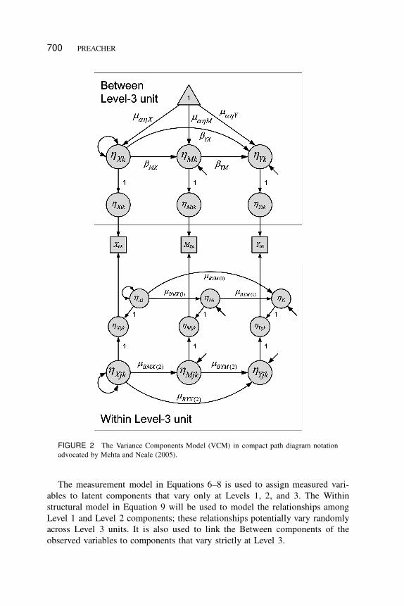
across Level 3 units. Figure 2 contains a compact path diagram illustrating

the VCM.

The VCM takes advantage of the isomorphism between a random-intercepts

multilevel model and a restricted confirmatory factor analysis (CFA) model with

unit factor loadings. Level 1 units are modeled as exchangeable with other

Level 1 units within the same Level 2 unit in precisely the same way that items

are exchangeable with other items that load on the same factor in CFA (Bauer,

2003; Curran, 2003; Mehta & Neale, 2005). It is possible to represent the VCM

in terms of B. O. Muthén and Asparouhov’s (2008) MSEM in the following

manner: The measurement model serves only to link the measured variables—

including Xijk , Mijk , and Yijk—to latent W and B components. Equation 6 is

an expansion of Equation 2a in which observed variables are linked to latent

Level 1, Level 2, and Level 3 components. In Equation 6, i D 1 or 2 to index

only two Level 1 units for simplicity. For example, Y1jk and Y2jk represent the

values of Y for the two Level 1 units within Level 2 unit j and Level 3 unit k.

Yijk D ƒjk˜jk D ŒX1jk X2jk M1jk M2jk Y1jk Y2jk�0; (6)

where

ƒjk D

2

64

1 0 0 0 0 0 1 0 0 0 0 0 0 0 0 1 0 0 0 0 0 0 0 0

0 1 0 0 0 0 0 1 0 0 0 0 0 0 0 0 1 0 0 0 0 0 0 0

0 0 1 0 0 0 0 0 1 0 0 0 0 0 0 0 0 1 0 0 0 0 0 0

0 0 0 1 0 0 0 0 0 1 0 0 0 0 0 0 0 0 1 0 0 0 0 0

0 0 0 0 1 0 0 0 0 0 1 0 0 0 0 0 0 0 0 1 0 0 0 0

0 0 0 0 0 1 0 0 0 0 0 1 0 0 0 0 0 0 0 0 1 0 0 0

––

––

––

––

– 3

75 (7)

˜0

jk D Œ˜X1jk ˜X2jk ˜M1jk ˜M 2jk ˜Y 1jk ˜Y 2jk ˜X1 ˜X2 ˜M1 ˜M 2 ˜Y 1 ˜Y 2 ˜Xjk ˜Mjk ˜Yjk

–– ˜X1k ˜X2k ˜M1k ˜M 2k ˜Y 1k ˜Y 2k ˜M k ˜Y k � (8)

Elements before the partition in ƒjk and ˜jk correspond to the Within model

(where Level 1 and Level 2 relationships will be modeled) and elements after

the partition correspond to the Between model (where Level 3 effects will be

modeled). The vector ©ijk is not used here but is available if the researcher

wishes to use latent variables with multiple indicators rather than measured

variables.

700 PREACHER

FIGURE 2 The Variance Components Model (VCM) in compact path diagram notation

advocated by Mehta and Neale (2005).

The measurement model in Equations 6–8 is used to assign measured vari-

ables to latent components that vary only at Levels 1, 2, and 3. The Within

structural model in Equation 9 will be used to model the relationships among

Level 1 and Level 2 components; these relationships potentially vary randomly

across Level 3 units. It is also used to link the Between components of the

observed variables to components that vary strictly at Level 3.


˜j

kD

’k

CB

k˜

jk

C—

jk

D

2 6 6 6 6 6 6 6 6 6 6 6 6 6 6 6 6 6 6 6 6 6 6 4

˜X

1jk

˜X

2jk

˜M

1jk

˜M

2jk

˜Y

1jk

˜Y

2jk

˜X

1

˜X

2

˜M

1

˜M

2

˜Y

1

˜Y

2

˜X

jk

˜M

jk

˜Y

jk

––

–˜

X1k

˜X

2k

˜M

1k

˜M

2k

˜Y

1k

˜Y

2k

˜X

k

˜M

k

˜Y

k

3 7 7 7 7 7 7 7 7 7 7 7 7 7 7 7 7 7 7 7 7 7 7 5

D

2 6 6 6 6 6 6 6 6 6 6 6 6 6 6 6 6 6 6 6 6 6 6 4

0 0 0 0 0 0 0 0 0 0 0 0 0 0 0–

––

0 0 0 0 0 0

’˜

Xk

’˜

Mk

’˜

Yk

3 7 7 7 7 7 7 7 7 7 7 7 7 7 7 7 7 7 7 7 7 7 7 5

C

2 6 6 6 6 6 6 6 6 6 6 6 6 6 6 6 6 6 6 6 6 6 6 4

00

00

00

00

00

00

10

00

00

00

00

00

00

00

00

00

00

00

10

00

00

00

00

00

00

00

00

00

00

00

01

00

00

00

00

00

00

00

00

00

00

00

01

00

00

00

00

00

00

00

00

00

00

00

00

10

00

00

00

00

00

00

00

00

00

00

00

10

00

00

00

00

00

00

00

00

00

00

00

00

00

00

00

00

00

00

00

00

00

00

00

00

00

00

00

00

00

00

00

BM

Xj

k0

00

00

00

00

00

00

00

00

00

00

00

0B

MX

jk

00

00

00

00

00

00

00

00

00

00

00

BY

Xj

k0

BY

Mj

k0

00

00

00

00

00

00

00

00

00

00

0B

YX

jk

0B

YM

jk

00

00

00

00

00

00

00

00

00

00

00

00

00

00

00

00

00

00

00

00

00

00

00

00

00

BM

Xk

00

00

00

00

00

0

00

00

00

00

00

00

BY

Xk

BY

Mk

00

00

00

00

00

––

––

––

––

––

––

––

––

––

––

––

––

––

––

––

––

––

––

––

––

––

––

––

––

––

––

––

00

00

00

00

00

00

00

00

00

00

00

00

00

00

00

00

00

00

00

00

00

00

00

00

00

00

00

00

00

00

00

00

00

00

00

00

00

00

00

00

00

00

00

00

00

00

00

00

00

00

00

00

00

00

00

00

00

00

00

00

00

00

00

00

00

00

00

00

00

00

00

00

00

00

00

00

00

00

00

00

00

00

00

00

00

00

00

00

00

00

00

00

00

00

00

00

00

00

00

00

00

00

00

00

00

00

00

00

––––––––––––––––––––––––––––––––

3 7 7 7 7 7 7 7 7 7 7 7 7 7 7 7 7 7 7 7 7 7 7 5

2 6 6 6 6 6 6 6 6 6 6 6 6 6 6 6 6 6 6 6 6 6 4

˜X

1jk

˜X

2jk

˜M

1jk

˜M

2jk

˜Y

1jk

˜Y

2jk

˜X

1

˜X

2

˜M

1

˜M

2

˜Y

1

˜Y

2

˜X

jk

˜M

jk

˜Y

jk

––

–˜

X1k

˜X

2k

˜M

1k

˜M

2k

˜Y

1k

˜Y

2k

˜M

k

˜Y

k

3 7 7 7 7 7 7 7 7 7 7 7 7 7 7 7 7 7 7 7 7 7 5

C

2 6 6 6 6 6 6 6 6 6 6 6 6 6 6 6 6 6 6 6 6 6 6 4

0 0 0 0 0 0

— X1

— X2

— M1

— M2

— Y1

— Y2

— Xj

k

— Mj

k

— Yj

k–

––

0 0 0 0 0 0 0 0 0

3 7 7 7 7 7 7 7 7 7 7 7 7 7 7 7 7 7 7 7 7 7 7 5

(9)

702 PREACHER

In Equation 9, the Within latent components of the observed variables Mijk

are regressed on the latent components of Xijk , and the latent components of Yijk

are regressed on the latent components of Xijk and Mijk . These slopes (BMXjk ,

BYXjk, and BYMjk ) represent strictly Level 1 effects that may vary randomly

across Level 3 units (but not across Level 2 units). The latent within components

in the VCM do not have residuals—their variance is divided completely into

latent Level 1 and Level 2 components. The latent Level 1 components (˜X1

through ˜Y 2) may be regressed on one another, and the latent Level 2 components

(˜Xjk , ˜Mjk , and ˜Yjk) may be regressed on one another. The residuals of these

latent components (—X1 through —Y 2 for Level 1 and —Xjk , —Mjk , and —Yjk for

Level 2) vary according to

—jk � MVN

0

BBBBBBBBBBBBBB@

2

666666666666664

0„ƒ‚…

6�1

0

0

0

0

0

0

0

0

0– – – –

0„ƒ‚…

9�1

3

777777777777775

;

2

66666666666664

0„ƒ‚…

6�6

0 ¢2Xjk

0 0 ¢2Xjk

0 0 0 ¢2Mjk

0 0 0 0 ¢2Mjk

0 0 0 0 0 ¢2Yjk

0 0 0 0 0 0 ¢2Yjk

‰Xk

0„ƒ‚…

3�1

0„ƒ‚…

3�6

0 ‰M k

0 0 ‰Y k– – – – – – – – – – – – – – – – – – – – – – – – – – – – – – – – – – – – – – – –

0„ƒ‚…

9�1

0„ƒ‚…

9�6

0„ƒ‚…

9�3

0„ƒ‚…

9�9––

––

––

––

––

––

––

––

––

––

––

––

3

77777777777775

1

CCCCCCCCCCCCCCA

:

(10)

In Equation 10, ¢2Xjk , ¢2

Mjk , and ¢2Yjk are Level 1 (residual) variances for the

subscripted variables, and ‰Xk , ‰Mk , and ‰Y k are Level 2 (residual) variances.

These variances cannot themselves vary at higher levels in B. O. Muthén and

Asparouhov’s (2008) MSEM framework. Residuals from Level 1 cannot covary

with residuals from Level 2.

Finally, the Between structural model in Equation 11 is used to model the

relationships among the Level 1 and Level 2 random effects. All of the random

elements from parameter matrices at Levels 1 and 2 (random intercepts and

slopes from ’k and Bk in Equation 9) are stacked into the vector ˜k . Means

and intercepts of these random effects populate the mean vector �, and the

random intercepts ’˜Xk , ’˜Mk , and ’˜Y k (representing strictly Level 3 variability

in X , M , and Y , respectively) are regressed on one another in matrix “. The

vector � also contains the means of Level 1 slopes in �BMX.1/, �BYX.1/, and

�BYM.1/. Thus, the Between structural model contains the strictly Level 1 slopes

(e.g., �BMX.1/), the strictly Level 2 slopes (e.g., �BMX.2/), and the strictly

Level 3 slopes (e.g., “MX ).

Preacher

Rectangle

Preacher

Rectangle

Preacher

Text Box

3×6

Preacher

Text Box

9×6

Preacher

Line

Preacher

Line


˜k D � C “˜k C —k

D

2

6666666664

�BMX.1/

�BYX.1/

�BYM.1/

�BMX.2/

�BYX.2/

�BYM.2/

�’˜X

�’˜M

�’˜Y

3

7777777775

C

2

6666666664

0 0 0 0 0 0 0 0 0

0 0 0 0 0 0 0 0 0

0 0 0 0 0 0 0 0 0

0 0 0 0 0 0 0 0 0

0 0 0 0 0 0 0 0 0

0 0 0 0 0 0 0 0 0

0 0 0 0 0 0 0 0 0

0 0 0 0 0 0 “MX 0 0

0 0 0 0 0 0 “YX “YM 0

3

7777777775

2

6666666664

BMXjk

BYXjk

BYMjk

BMXk

BYXk

BYMk

’˜Xk

’˜Mk

’˜Y k

3

7777777775

C

2

6666666664

—BMXjk

—BYXjk

—BYMjk

—BMXk

—BYXk

—BYMk

—’˜Xk

—’˜Mk

—’˜Y k

3

7777777775

(11)

The Between model residuals vary and covary according to

—k � MVN

0

BBBBBB@

2

6666664

00

00000

00

3

7777775

;

2

6666664

8

<

:

§11

§21 §22

§31 §32 §33

9

=

;

Level 3 (co)variances

of Level 1 random slopes

§41 §42 §43

§51 §52 §53

§61 §62 §63

8

<

:

§44

§54 §55

§64 §65 §66

9

=

;

Level 3 (co)variances

of Level 2 random slopes

§71 §72 §73 §74 §75 §76

§81 §82 §83 §84 §85 §86

§91 §92 §93 §94 §95 §96

8

<

:

§77

0 §88

0 0 §99

9

=

;

3

7777775

1

CCCCCCA

Variances of

Level 3 intercepts

(12)

The residual variances in the Between model may vary freely for random

coefficients or may be constrained to zero for fixed coefficients, as the situation

dictates.

Fitting the VCM requires software capable of fitting multilevel SEM with

random coefficients. Currently the only software in which this is practical is

Mplus (L. K. Muthén & Muthén, 1998–2010). The steps involved in specifying

the VCM are as follows:

1. Create a data set in which every row corresponds to a different Level 2

unit. Identify the maximum Level 2 cluster size .max.nj // and create that

many repeated measure variables each for Xijk , Mijk , and Yijk . Thus, there

will be 3 times as many columns as there are Level 1 units in the largest

Level 2 cluster. For Level 2 units containing fewer than max.nj / Level 1

units, any observations short of max.nj / will be treated as missing data.

Include an additional column denoting Level 3 cluster membership.

2. Allow Xijk , Mijk , and Yijk to load onto latent variables in the Within

model with unit loadings, and allow Xijk , Mijk , and Yijk to load onto

latent variables in the Between model with unit loadings. This partitions

the observed variables into latent components that vary strictly within and

strictly between Level 3 units.

704 PREACHER

3. Specify the Within model.

a. Allow the latent components of Xijk , Mijk , and Yijk to load onto

Level 2 intercept factors with unit loadings.

b. Allow each latent component of Xijk , Mijk , and Yijk to load onto its

own Level 1 latent variable in the Within model with unit loadings.

c. Regress the intercept factor for M onto the intercept factor for X , and

regress the intercept factor for Y onto the intercept factors for both X

and M .

d. Regress the Level 1 latent components of M onto corresponding Level 1

latent components of X , constraining these slopes to equality. Regress

the Level 1 latent components of Y onto corresponding Level 1 latent

components of X and M , constraining the X slopes to equality and

constraining the M slopes to equality.

4. Specify the Between model.


intercept factors with unit loadings.

b. Regress the intercept factor for M onto the intercept factor for X , and


and M .

There are potentially three indirect effects in the VCM, which can be labeled

the Level 1, Level 2, and Level 3 indirect effects. The Level 1 and Level 2

indirect effects may involve slopes that vary at Level 3. If both component

slopes of either the Level 1 or Level 2 indirect effect vary at Level 3, then the

indirect effect involves a Level 3 covariance term in addition to the usual product

of coefficients (Goodman, 1960). The Level 1 indirect effect is quantified as

¨VCM1 D �BMX.1/�BYM.1/ C§31 and is interpreted as the indirect effect of Xijk

on Yijk via Mijk after controlling for Level 2 and Level 3 cluster membership.

Its estimation assumes that there is no Level 2 covariance between the Within

slopes BMXjk and BYMjk . The Level 2 indirect effect is quantified as ¨VCM2 D

�BMX.2/�BYM.2/ C §64 and is interpreted as the indirect effect of the Level 2

cluster mean of Xijk on the Level 2 cluster mean of Yijk via the Level 2 cluster

mean of Mijk after controlling for Level 3 cluster membership. The Level 3

indirect effect is quantified as ¨VCM3 D “MX “YM and is interpreted as the

indirect effect of the Level 3 cluster mean of Xijk on the Level 3 cluster mean

of Yijk via the Level 3 cluster mean of Mijk .

Advantages. The VCM has several advantages over existing methods for

assessing mediation in three-level data. First, it can be used to estimate separate

effects at each level rather than a single conflated effect (as in MLM). Second,

it accommodates dependence due to nesting within both Level 2 and Level 3

clusters. Third, it can accommodate Level 1 and Level 2 slopes that may be

random at Level 3. Fourth, because ¨VCM1 , ¨VCM2 , and ¨VCM3 are estimated


using latent components of Xijk , Mijk , and Yijk that vary strictly within Levels

1, 2, and 3, these slopes are not conflated across levels; nor are they biased due

to using observed cluster means. Fifth, it can accommodate a variety of Level 1

residual covariance structures (independence was assumed here). Sixth, it can

be estimated using existing software intended for two-level models. Seventh,

because full information maximum likelihood (FIML) estimation is used, it

can accommodate clusters of different sizes simply by considering clusters

with fewer than the maximum observed number of cases as containing missing

data. Eighth, it can be extended to accommodate latent variables with multiple

indicators. Finally, it can be expanded to accommodate other mediation models,

such as longitudinal or multiple-mediator models.

Disadvantages. A disadvantage of the VCM is that Level 1 slopes may

not be specified as random across Level 2 units (only across Level 3 units). If

the Level 1 slopes really do vary across Level 2 units, the model is misspecified

and bias likely will result.

Method 2: Contextual Effects Model (CEM)

The second method is termed the Contextual Effects Model (CEM). As with

the VCM, CEM involves partitioning of variance into components. However,

the components in CEM correspond to purely Level 3 variance (in the Between

model) and purely Level 2 and purely Within (Level 1 C Level 2) components.

Within latent components (which contain both Level 1 and Level 2 variance)

are directly regressed onto other Within latent components (see Figure 3).

Fitting the CEM proceeds much as with the VCM. The CEM can be rep-

resented in terms of B. O. Muthén and Asparouhov’s (2008) MSEM in the

following manner: As with the VCM, the measurement model serves only to link

the measured variables to latent Within and Between components. In Equation

13, i D 1 or 2 to index only two Level 1 units.

Yijk D ƒjk˜jk D ŒX1jk X2jk M1jk M2jk Y1jk Y2jk�0; (13)

where

ƒjk D

2

6666664

1 0 0 0 0 0 0 0 0 1 0 0 0 0 0 0 0 0

0 1 0 0 0 0 0 0 0 0 1 0 0 0 0 0 0 0

0 0 1 0 0 0 0 0 0 0 0 1 0 0 0 0 0 0

0 0 0 1 0 0 0 0 0 0 0 0 1 0 0 0 0 0

0 0 0 0 1 0 0 0 0 0 0 0 0 1 0 0 0 0

0 0 0 0 0 1 0 0 0 0 0 0 0 0 1 0 0 0––

––

––

––

–– 3

7777775

(14)

˜0

jk D Œ˜X1jk ˜X2jk ˜M1jk ˜M2jk ˜Y 1jk ˜Y 2jk ˜Xjk ˜Mjk ˜Yjk

–– ˜X1k ˜X2k ˜M1k ˜M2k ˜Y 1k ˜Y 2k ˜Xk ˜Mk ˜Y k � (15)

706 PREACHER

FIGURE 3 The Contextual Effects Model (CEM) in compact path diagram notation

advocated by Mehta and Neale (2005).

Elements before the partition in ƒjk and ˜jk again correspond to the Within

model (Level 1 and Level 2) and elements after the partition correspond to the

Between model (Level 3). The vector ©ijk is again omitted for simplicity.

The Within structural model in Equation 16 will be used to model the rela-

tionships among W components; these relationships can vary randomly across


Level 3 units. It is also used to link the B components of the observed variables

to components that vary strictly at Level 3.

˜jk D ’k C Bk˜jk C —jk

D

2

6666666666666664

0

0

0

0

0

0

0

0

0– – –

0

0

0

0

0

0

’˜Xk

’˜M k

’˜Y k

3

7777777777777775

C

2

6666666666666664

0 0 0 0 0 0 1 0 0 0 0 0 0 0 0 0 0 0

0 0 0 0 0 0 1 0 0 0 0 0 0 0 0 0 0 0

BMXjk 0 0 0 0 0 0 1 0 0 0 0 0 0 0 0 0 0

0 BMXjk 0 0 0 0 0 1 0 0 0 0 0 0 0 0 0 0

BYXjk 0 BYMjk 0 0 0 0 0 1 0 0 0 0 0 0 0 0 0

0 BYXjk 0 BYMjk 0 0 0 0 1 0 0 0 0 0 0 0 0 0

0 0 0 0 0 0 0 0 0 0 0 0 0 0 0 0 0 0

0 0 0 0 0 0 BMXk 0 0 0 0 0 0 0 0 0 0 0

0 0 0 0 0 0 BYXk BYM k 0 0 0 0 0 0 0 0 0 0– – – – – – – – – – – – – – – – – – – – – – – – – – – – – – – – – – – – – – – – – – – – – –

0 0 0 0 0 0 0 0 0 0 0 0 0 0 0 1 0 0

0 0 0 0 0 0 0 0 0 0 0 0 0 0 0 1 0 0

0 0 0 0 0 0 0 0 0 0 0 0 0 0 0 0 1 0

0 0 0 0 0 0 0 0 0 0 0 0 0 0 0 0 1 0

0 0 0 0 0 0 0 0 0 0 0 0 0 0 0 0 0 1

0 0 0 0 0 0 0 0 0 0 0 0 0 0 0 0 0 1

0 0 0 0 0 0 0 0 0 0 0 0 0 0 0 0 0 0

0 0 0 0 0 0 0 0 0 0 0 0 0 0 0 0 0 0

0 0 0 0 0 0 0 0 0 0 0 0 0 0 0 0 0 0––

––

––

––

––

––

––

––

––

––

––

–– 3

7777777777777775

2

6666666666666664

˜X1jk

˜X2jk

˜M1jk

˜M 2jk

˜Y 1jk

˜Y 2jk

˜Xjk

˜Mjk

˜Yjk– – –˜X1k

˜X2k

˜M1k

˜M 2k

˜Y 1k

˜Y 2k

˜Xk

˜M k

˜Y k

3

7777777777777775

C

2

6666666666666664

—X1

—X2

—M1

—M 2

—Y 1

—Y 2

—Xjk

—Mjk

—Yjk– – –

0

0

0

0

0

0

0

0

0

3

7777777777777775

(16)

In Equation 16, the W components of the observed Mijk are regressed on the

W components of Xijk , and the W components of Yijk are regressed on the

W components of Xijk and Mijk . Even though these latent components contain

both Level 1 and Level 2 components, they are also regressed on Level 2 latent

variables indirectly through unit loadings on the purely Level 2 components

˜Xjk and ˜Mjk , which in turn are regressed on one another. Therefore, after

controlling for the Level 2 components, the remaining effects (BMXjk , BYXjk,

and BYMjk) are purely Level 1 effects. However, the structural effects of the

Level 2 components of the indirect effect (BMXk and BYMk) no longer represent

strictly Level 2 effects but rather contextual effects—differences between purely

Level 1 and purely Level 2 effects (Lüdtke et al., 2008; Raudenbush & Bryk,

2002). Any of these effects may potentially vary randomly across Level 3 units

(but not Level 2 units). The residuals of these latent Level 1 and Level 2

components (—X1 through —Y 2 for Level 1 and —Xjk , —Mjk , and —Yjk for Level 2)

708 PREACHER

vary according to

—jk � MVN

0

BBBBBBBBBBB@

2

666666666664

0

0

0

0

0

0

0

0

0– – –

0„ƒ‚…

9�1

3

777777777775

;

2

66666666664

¢2Xjk

0 ¢2Xjk

0 0 ¢2Mjk

0 0 0 ¢2Mjk

0 0 0 0 ¢2Yjk

0 0 0 0 0 ¢2Yjk

‰Xk

0„ƒ‚…

3�6

0 ‰M k

0 0 ‰Y k– – – – – – – – – – – – – – – – – – – – – – – – – – – – – – – – – – –

0„ƒ‚…

9�6

0„ƒ‚…

9�3

0„ƒ‚…

9�9––

––

––

––

––

––

––

––

––

––

3

77777777775

1

CCCCCCCCCCCA

:

(17)

Finally, the Between structural model is used to model the relationships

among the Level 1 and contextual random effects. The Between model is

identical to Equation 11, so it is not repeated here. Similarly, the Between

model residuals in CEM vary and covary according to Equation 12 save that the

(co)variances of Level 2 slopes are actually (co)variances of contextual effects

in CEM.

The steps involved in specifying the CEM are as follows:



many repeated measure variables each for Xijk , Mijk , and Yijk . Thus, there

will be 3 times as many columns as there are Level 1 units in the largest

Level 2 cluster. For Level 2 units containing fewer than max.nj / Level 1

units, any observations short of max.nj / will be treated as missing data.

Include an additional column denoting Level 3 cluster membership.

2. Allow Xijk , Mijk , and Yijk to load onto latent variables in the Within

model with unit loadings, and allow Xijk , Mijk , and Yijk to load onto

latent variables in the Between model with unit loadings. This partitions

the observed variables into latent components that vary strictly within and

strictly between Level 3 units.

3. Specify the Within model.


Level 2 intercept factors with unit loadings.

b. Regress the latent components of M onto corresponding Level 1 latent

components of X , constraining these slopes to equality. Regress the

Level 1 latent components of Y onto corresponding Level 1 latent

components of X and M , constraining the X slopes to equality and con-

straining the M slopes to equality. These slopes represent the Level 1

effects.


c. Regress the intercept factor for M onto the intercept factor for X , and


and M . The slopes BMXk and BYMk represent contextual effects.

4. Specify the Between model.


intercept factors with unit loadings.

b. Regress the intercept factor for M onto the intercept factor for X , and


and M .

The Level 1 and Level 3 indirect effects in the CEM are computed and

interpreted in the same way as in the VCM. However, the Level 2 indirect effect

must be computed by first adding the Level 1 and contextual slopes prior to

multiplying. These indirect effects are denoted ¨CEM1, ¨CEM2, and ¨CEM3,

with ¨CEM2 D .�BMX.1/ C �BMX.2//.�BYM.1/ C �BYM.2// for most models

(CEM is not recommended for models with both Level 2 slopes random due to

interpretational difficulties associated with the contextual effect covariance).

Advantages. CEM has the same advantages as VCM and is simpler to

specify because it involves potentially many fewer latent variables. CEM also

takes less time to converge, and estimation may be more stable.

Disadvantages. As with VCM, Level 1 slopes in CEM may not be spec-

ified as random across Level 2 units (only across Level 3 units). As pointed

out earlier, even though CEM is statistically equivalent to VCM, the Level 2

components of the indirect effect are contextual effects, so special steps must

be taken when computing the Level 2 indirect effect.

Method 3: Conflated Coefficients Model (CCM)

The third proposed method, termed the Conflated Coefficients Model (CCM),

is analogous to a traditional three-level MLM with conflated slopes. That is,

CCM is a mediation model characterized by random intercepts and slopes that

potentially may vary and covary across both Level 2 and Level 3 units, but

only single, conflated estimates of slope means are available. As a traditional

three-level random coefficients model, the CCM is also a three-level extension

to the two-level mediation model of Bauer et al. (2006). Because it requires only

single-level SEM architecture to be specified, it is not considered an application

of B. O. Muthén and Asparouhov’s (2008) approach to MSEM.

It has been known for some time how to use single-level SEM architecture to

specify a two-level model in the context of models for longitudinal data. Latent

growth curve modeling (LGM; Bollen & Curran, 2006; Meredith & Tisak, 1990)

710 PREACHER

is the most prominent example of this practice. In LGM, fixed factor loadings

in ƒ contain values of the Level 1 predictor timeij , and random coefficients

(intercepts, slopes) are represented in the model by latent variables. LGM is

identical in virtually every way to MLM models for longitudinal data but can

be extended flexibly. Bauer (2003), Mehta and Neale (2005), and Mehta and

West (2000) generalized the overlap between SEM and MLM by showing how

any Level 1 predictor (not just time) can be incorporated into loadings using

definition variables (in Mx; Neale, Boker, Xie, & Maes, 2003) or CONSTRAINT

variables (Mplus; L. K. Muthén & Muthén, 1998–2010) using FIML estimation.

This method allows the factor loadings to differ from case to case, just as values

of a Level 1 predictor may vary from Level 1 unit to Level 1 unit in MLM. In

fact, virtually any two-level model can be fit in the single-level SEM framework

by means of model specification and careful data management.

This method of fitting a two-level model within single-level SEM generalizes

directly to fitting a three-level model by combining the insights of Duncan et al.

(2002) with those of Bauer (2003) and Mehta and West (2000). Duncan et al.

(2002) specified a four-level growth model within the MSEM framework by

separating repeated measures into within- and between-region components. The

Between model was used to model region-level components of growth (Level 4),

whereas the Within model was used to model the effect of time on adolescent

substance use (Level 1), between-person variation in the growth coefficients

(Level 2), and family-level variability in the person-level coefficients (Level 3).

Their Within model was thus a creative use of McArdle’s (1988) factor-of-curves

model. In the factor-of-curves model, intercepts and slopes load onto higher

level intercept and slope factors. The model requires as many simultaneously

estimated latent growth curve submodels as there are Level 2 units in the biggest

Level 3 unit.

The model of Duncan et al. (2002) is limited to the growth curve context in

which there is a single Level 1 predictor (time) and a single outcome (substance

use). The model is intended for data that are balanced on time, so factor loadings

merely need to be constrained equal to the values of time that all subjects have in

common. On the other hand, the model suggested here is somewhat simpler than

Duncan et al.’s (2002) in that it involves only three levels rather than four and

does not take advantage of the full MSEM (i.e., the model accounts for three-

level clustering using only single-level SEM architecture rather than the between-

within decomposition of variance). By incorporating definition variables after the

manner suggested by Bauer (2003) and Mehta and West (2000), it is possible

to construct a model that is not restricted to data that are balanced with respect

to the Level 1 predictor(s), not restricted to repeated measures data (i.e., with

time as a Level 1 predictor), and not restricted to a single Level 1 predictor and

outcome. It is possible to incorporate definition variables into the factor loading

matrix such that any Level 1 predictor and outcome variables may be included.


For simplicity, the model is represented in equation form for the special case

of two Level 1 units nested within each of two Level 2 units, which in turn are

nested within an arbitrary number of Level 3 units. The Level 1 “measurement”

equation (for the simple case explored here) is

Yijk D ƒjk˜jk C ©ijk D ŒM11k M21k Y11k Y21k M12k M22k Y12k Y22k�0;

(18)

where

ƒjk D

2

66666664

1 ŒX11k � 0 0 0 0 0 0 0 0 0 0 0 0 0

1 ŒX21k � 0 0 0 0 0 0 0 0 0 0 0 0 0

0 0 1 ŒX11k � ŒM11k � 0 0 0 0 0 0 0 0 0 0

0 0 1 ŒX21k � ŒM21k � 0 0 0 0 0 0 0 0 0 0

0 0 0 0 0 1 ŒX12k � 0 0 0 0 0 0 0 0

0 0 0 0 0 1 ŒX22k � 0 0 0 0 0 0 0 0

0 0 0 0 0 0 0 1 ŒX12k � ŒM12k � 0 0 0 0 0

0 0 0 0 0 0 0 1 ŒX22k � ŒM22k � 0 0 0 0 0

3

77777775

(19)

˜0

jk D Œ˜M1k ˜MX1k ˜Y 1k ˜YX1k ˜YM1k ˜M2k ˜MX2k ˜Y 2k

˜YX2k ˜YM2k ˜Mk ˜MXk ˜Y k ˜YXk ˜YMk � (20)

©0

ijk D Œ©M11k ©M21k ©Y 11k ©Y 21k ©M12k ©M22k ©Y 12k ©Y 22k �: (21)

In Equation 18, M11k and M21k are the observed values of Mijk for the two

Level 1 units nested in the first Level 2 unit (similar for observations of Yijk).

Elements of the loading matrix ƒjk in [.] symbols are definition variables (in

Mx) or CONSTRAINT variables (in Mplus) and represent values of Xijk and

Mijk that can differ from Level 1 unit to Level 1 unit. Elements of ˜jk represent

Level 2 random coefficients: ˜Mjk is the Level 2 random intercept for the first

Level 1 unit’s Mijk equation, ˜MX2k is the random slope for Mijk regressed

onto Xijk for the second Level 2 unit, and so on. Elements of ©ijk are Level 1

disturbance terms, distributed as

©ij � MVN

0

BBBBBBBBBB@

2

66666666664

0

0

0

0

0

0

0

0

3

77777777775

;

2

66666666664

¢2©M 0 0 0 0 0 0 0

0 ¢2©M 0 0 0 0 0 0

0 0 ¢2©Y 0 0 0 0 0

0 0 0 ¢2©Y 0 0 0 0

0 0 0 0 ¢2©M 0 0 0

0 0 0 0 0 ¢2©M 0 0

0 0 0 0 0 0 ¢2©Y 0

0 0 0 0 0 0 0 ¢2©Y

3

77777777775

1

CCCCCCCCCCA

: (22)

In the structural model (Equation 23), the Level 2 random coefficients are linked

with Level 3 random coefficients (˜Mk through ˜YMk ) with unit loadings in B

712 PREACHER

and have associated Level 2 residuals (—M1k through —YM2k). The Level 3 random

coefficients, in turn, are modeled as functions of means (�M through �YM ) and

Level 3 residuals (—Mk through —YMk).

˜jk D ’ C B˜jk C —jk D

2

666666666666664

00000

00000

�M

�MX

�Y

�YX

�YM

3

777777777777775

C

2

666666666666664

0 0 0 0 0 0 0 0 0 0 1 0 0 0 00 0 0 0 0 0 0 0 0 0 0 1 0 0 00 0 0 0 0 0 0 0 0 0 0 0 1 0 00 0 0 0 0 0 0 0 0 0 0 0 0 1 00 0 0 0 0 0 0 0 0 0 0 0 0 0 1

0 0 0 0 0 0 0 0 0 0 1 0 0 0 00 0 0 0 0 0 0 0 0 0 0 1 0 0 00 0 0 0 0 0 0 0 0 0 0 0 1 0 00 0 0 0 0 0 0 0 0 0 0 0 0 1 00 0 0 0 0 0 0 0 0 0 0 0 0 0 1

0 0 0 0 0 0 0 0 0 0 0 0 0 0 00 0 0 0 0 0 0 0 0 0 0 0 0 0 00 0 0 0 0 0 0 0 0 0 0 0 0 0 00 0 0 0 0 0 0 0 0 0 0 0 0 0 00 0 0 0 0 0 0 0 0 0 0 0 0 0 0

3

777777777777775

2

666666666666664

˜M1k

˜MX1k

˜Y 1k

˜YX1k

˜YM1k

˜M 2k

˜MX2k

˜Y 2k

˜YX2k

˜YM 2k

˜M k

˜MXk

˜Y k

˜YXk

˜YM k

3

777777777777775

C

2

666666666666664

—M1k

—MX1k

—Y 1k

—YX1k

—YM1k

—M 2k

—MX2k

—Y 2k

—YX2k

—YM 2k

—M k

—MXk

—Y k

—YXk

—YM k

3

777777777777775

:

(23)

The Level 2 and Level 3 residuals (in the case of only two Level 2 units per

Level 3 unit) vary and covary according to

—jk � MVN

0

BBBBBBBBBBB@

2

666666666664

0

0

0

0

0

0

0

0

0

0

0

0

0

0

0

3

777777777775

;

2

666666666664

‰11

‰21 ‰22

‰31 ‰32 ‰33

‰41 ‰42 ‰43 ‰44

‰51 ‰52 ‰53 ‰54 ‰55

‰11

‰21 ‰22

‰31 ‰32 ‰33

‰41 ‰42 ‰43 ‰44

‰51 ‰52 ‰53 ‰54 ‰55

‰11

‰21 ‰22

‰31 ‰32 ‰33

‰41 ‰42 ‰43 ‰44

‰51 ‰52 ‰53 ‰54 ‰55

3

777777777775

1

CCCCCCCCCCCA

:

(24)

In Equation 24, all Level 2 units are constrained to have the same residual

covariance structure. The final 5�5 submatrix on the main diagonal of Equation

24 contains Level 3 variances and covariances.

If variability across Level 3 coefficients were to be ignored, the model

defined by Equations 18-24 would yield results equivalent to the multilevel

mediation model for 1-1-1 designs described by Bauer et al. (2006); in fact, this

demonstrates how the MLM-based procedure of Bauer et al. may be specified

using single-level SEM. Any of the random coefficients may be treated as fixed

coefficients by constraining elements of Equation 24 to zero as needed. The

three-level model described in Equations 18–24 is not identified for only two


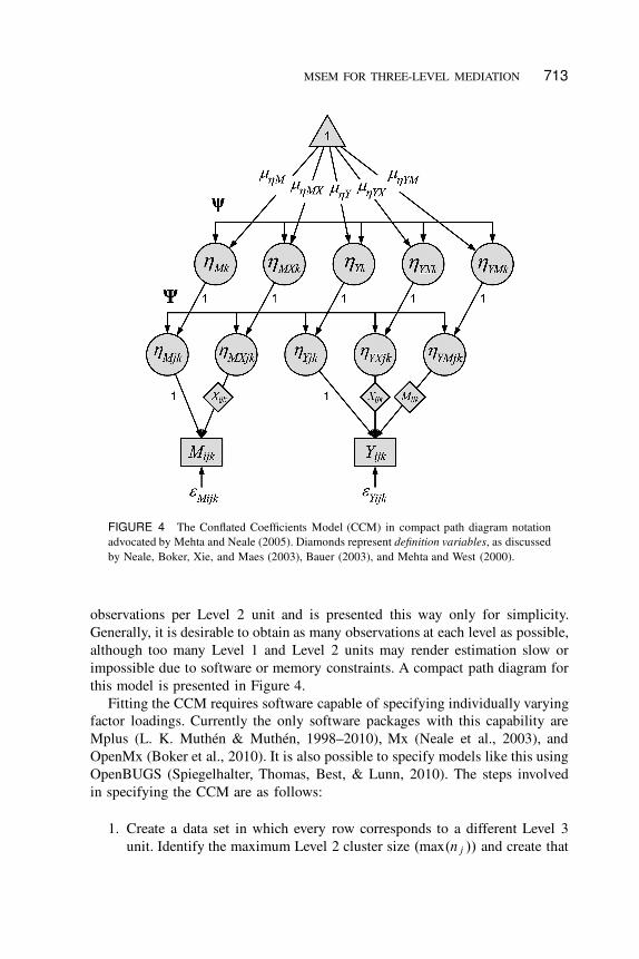
FIGURE 4 The Conflated Coefficients Model (CCM) in compact path diagram notation

advocated by Mehta and Neale (2005). Diamonds represent definition variables, as discussed

by Neale, Boker, Xie, and Maes (2003), Bauer (2003), and Mehta and West (2000).

observations per Level 2 unit and is presented this way only for simplicity.

Generally, it is desirable to obtain as many observations at each level as possible,

although too many Level 1 and Level 2 units may render estimation slow or

impossible due to software or memory constraints. A compact path diagram for

this model is presented in Figure 4.

Fitting the CCM requires software capable of specifying individually varying

factor loadings. Currently the only software packages with this capability are

Mplus (L. K. Muthén & Muthén, 1998–2010), Mx (Neale et al., 2003), and

OpenMx (Boker et al., 2010). It is also possible to specify models like this using

OpenBUGS (Spiegelhalter, Thomas, Best, & Lunn, 2010). The steps involved

in specifying the CCM are as follows:



714 PREACHER

many repeated measure variables each for Mijk, Yijk, ŒXijk �, and ŒMijk �

for each Level 2 unit in wide format. For Level 2 units containing fewer

than max.nj / Level 1 units, any observations short of max(nj ) will be

treated as missing data. Thus, there will be 4 times as many columns as

there are Level 1 units in the largest Level 2 cluster.

2. Allow repeated measures of Mijk to load onto an intercept factor with unit

loadings and a slope factor with loadings equal to ŒXijk �. This can be done

in Mplus by duplicating Xijk variables in the data set and declaring one

set as CONSTRAINT variables or in Mx or OpenMx by treating ŒXijk �

as definition variables.

3. Allow repeated measures of Yijk to load onto an intercept factor with unit

loadings, a slope factor with loadings equal to ŒXijk�, and another slope

factor with loadings equal to ŒMijk�.

4. Estimate variances and covariances for the random intercepts and slopes

separately for the submodel corresponding to each Level 2 unit and con-

strain covariances among random coefficients for different Level 2 units

to zero. Constrain corresponding variance and covariance parameters to

equality across Level 2 units (e.g., the variance of ˜M1k should be con-

strained to equal the variance of ˜M2k , ˜M3k , etc.).

5. Allow all Level 2 random coefficients of a given type to load onto Level 3

random coefficient latent variables (e.g., ˜YX1k and ˜YX2k will load onto

the same higher order factor ˜YXk) with unit loadings.

6. Estimate means, variances, and covariances for the Level 3 random coef-

ficients.

The indirect effect in the CCM is quantified as ¨C CM D �MX �YM C ‰52 C §52

and is interpreted as the overall indirect effect of Xijk on Yijk via Mijk . The

two covariance terms in the expression for ¨C CM derive from the fact that

indirect effects are equal to the product of the means of the constituent slopes

plus the covariance of the random portions of those slopes (Goodman, 1960).

The estimated slopes composing ¨CRC can be represented as weighted averages

(conflations) of the Level 1, Level 2, and Level 3 effects that were estimated in

the unconflated three-level models discussed earlier.

Advantages. The CCM (Equations 18–24) is identical to the corresponding

representation in three-level MLM. Relative to models that do not consider

the multilevel nature of the data, the CCM has several advantages. First, it

accommodates local dependence due to nesting within both Level 2 and Level 3

units using only single-level SEM architecture. Second, it can accommodate

Level 1 slopes that may be random at Level 2 and/or Level 3 and Level 2

slopes that may be random at Level 3 (an advantage not shared by VCM or

CEM). Third, it can accommodate a variety of Level 1 residual covariance


structures (independence was assumed here). Fourth, it can be estimated using

some existing software intended for single-level SEM. Fifth, because FIML

estimation is used, it can accommodate clusters of different sizes simply by

considering clusters with fewer than max.nj / cases as containing missing data.

Sixth, although this feature was not illustrated here, CCM can accommodate

latent variables with multiple indicators. Seventh, even though the CCM in

Equations 18–24 is an extension of the traditional three-variable X ! M ! Y

mediation model, it can be expanded to accommodate other mediation mod-

els, such as models for longitudinal mediation or models involving multiple

mediators.

The CCM contains, as special cases, most existing multilevel models for me-

diation so far suggested in the literature. It is a direct extension of Bauer et al.’s

(2006) model for two-level mediation in 1-1-1 designs that can accommodate

nesting in Level 3 units. In addition, models for 2-1-1 and 2-2-1 discussed by

Kenny, Kashy, and Bolger (1998), Krull and MacKinnon (1999, 2001), Pituch

and Stapleton (2008), and Pituch et al. (2006) can be considered special cases as

can the three-level models described by Pituch et al. (2010). A final advantage

of CCM is that, unlike with traditional MLM, CCM permits the model to be

embedded in a larger causal model.

Disadvantages. There are at least two disadvantages to the CCM that

limit its usefulness. First, the indirect effect .¨C CM / is based on slopes that

are conflated across levels. As is well known in the MLM literature, 1-1 slopes

in two-level models are weighted averages of W and B slopes. If these strictly

Level 1 and Level 2 slopes differ, then the conflated slope will be difficult to

interpret. The problem is more complex in three-level data, where the single

estimated slope is a conflation of Level 1, Level 2, and Level 3 components,

which may differ not only in magnitude but also in sign. This clearly poses

a problem for the interpretation of indirect effects based on these conflated

slopes.

A second disadvantage is that CCM can involve a prohibitively large number

of measured and latent variables. For balanced designs, the number of measured

variables will be nj � J , where nj is the number of Level 1 units within a

Level 2 unit and J is the number of Level 2 units. For example, a design with

10 repeated measures and 60 Level 2 units would have 600 measured variables.

Clearly such a model would be difficult or impossible to estimate, so there are

real limits on the total number of Level 1 units that can be accommodated by

CCM (Rabe-Hesketh et al., 2004). The CCM finds its greatest utility in situations

with few Level 1 units per Level 2 unit, few Level 2 units per Level 3 unit, and

many Level 3 units. If the full CCM (with all coefficients random at Levels 2

and 3) cannot be fit to a given data set, it may still be possible to fit parsimonious

special cases with only a few random coefficients.

716 PREACHER

TABLE 1

Advantages Associated With VCM, CEM, and CCM Methods of Assessing

Mediation in Multilevel Data via MSEM

VCM CEM CCM

Unconflated slopes � �

L1 slopes random at L2? �

L1 slopes random at L3? � � �

L2 slopes random at L3? � �

Contextual effect estimated and random at L3? �

Accommodates dependence � � �

Many residual covariance structures possible � � �

Can be estimated in 2-level SEM software � � �

Unbalanced clusters � � �

Latent variables w/multiple indicators � � �

Model fit possible � � �

Note. VCM D Variance Components Model; CEM D Contextual Effects Model;

CCM D Conflated Coefficients Model.

Advantages and Disadvantages of Each Method

To summarize, I have discussed three MSEM modeling strategies for assessing

mediation in three-level data. They include the Variance Components Model

(VCM), the Contextual Effects Model (CEM), and the Conflated Coefficients

Model (CCM). No one method is universally superior to the others. Rather,

different situations will call for different methods. Given the goal of discovering

at what level(s) effects are occurring, VCM and CEM are better suited than

CCM. However, it is not possible to let the Level 1 slopes vary across Level 2

units in VCM or CEM. CCM allows estimation of random slope variability at

Level 2 and/or Level 3 in a manner analogous to traditional MLM but conflates

the slope means across levels. CCM would allow estimating what would be

an ordinary three-level MLM (useful in its own right) but permits the limited

inclusion of latent variables, an improvement over traditional MLM. A chart

summarizing the relative advantages of VCM, CEM, and CCM is provided in

Table 1.

EXAMPLE(S) OF THREE-LEVEL MSEM FOR MEDIATION

Three examples are provided to illustrate some of the concepts described in this

article. All use data simulated to have a three-level structure.1

1Data, appendices, and syntax are available at the author’s website (http://quantpsy.org).


Example 1: Simulated Data Example for a 1-1-1 Design With

Balanced Clusters and Fixed Slopes for the VCM and CEM

Data were simulated to conform to a 1-1-1 design to illustrate the VCM and

CEM. Using Fortran, X , M , and Y were generated to conform to a three-level

nested structure with 10 Level 1 units within each Level 2 unit, and 10 Level 2

units within each of 800 Level 3 units, for a total sample size of 80,000. These

data may represent a three-stage random sample of schools, classrooms, and

students with fully balanced cluster sizes and no missing data. All slopes were

considered fixed. Population values for all parameters are included in Table 2

along with estimates of corresponding parameters under the VCM and CEM.

The generated sample data were modeled using Mplus 6.1 (L. K. Muthén &

Muthén, 1998–2010) with robust maximum likelihood estimation. Mplus code

for this example using VCM and CEM specifications is provided in online

Appendices A and B. For VCM and CEM, convergence was reached in ap-

proximately 5 s on a laptop computer with a 2.93 GHz dual-core processor

running Windows XP. In this simulated data set, there is a sizable proportion

of variance at each level for X , M , and Y . Furthermore, the sample size is

large enough to detect the indirect effect at each level. Confidence intervals

(CIs) were determined on the basis of Monte Carlo sampling distributions of

the indirect effect at each level (Bauer et al., 2006; MacKinnon, Lockwood, &

Williams, 2004) using point estimates and SEs taken from VCM. These CIs

were CI.¨VCM1/ D Œ:018; :021�, CI.¨VCM2/ D Œ:025; :041�, and CI.¨VCM3/ D

Œ:040; :102�. In this example, the indirect effect was recovered well by both

methods. VCM has an advantage over CEM in that the indirect effect for

Level 1 does not involve additional computations accounting for the fact that

the Level 2 effects are actually contextual effects. Thus, the VCM method can

be recommended as the method of first recourse in investigations of three-level

mediation of this type.

Example 2: Simulated Data Example for a 1-2-3 Design With

Unbalanced Clusters and Random Slopes for the VCM and CEM

Example 2 was designed to demonstrate some of the flexibility of the MSEM

approach relative to MLM. Using Fortran, X , M , and Y were generated to

conform to a three-level (specifically, 1-2-3) nested data structure with 350

Level 3 units. In each Level 3 unit there were between 2 and 14 Level 1 units,

and within each Level 2 unit there were between 5 and 17 Level 1 units, for

a total sample size of 30,490. The data may be thought of as representing

employees nested within teams, which in turn are nested within companies.

Team sizes ranged from 2 to 14, and the number of teams ranged from 5 to 17

per company. The researcher may be interested to know whether the effect of

718 PREACHER

TABLE 2

Population Values and Sample Estimates of Parameters

in a Three-Level Mediation Model for

1-1-1 Data (VCM and CEM)

Parameter Population VCM CEM

Level 1

�BMX.1/ .20 .198 (.004) .198 (.004)

�BYM.1/ .10 .097 (.004) .097 (.004)

�BYX.1/ .10 .102 (.004) .102 (.004)

¢2Xjk .34 .341 (.003) .341 (.003)

¢2Mjk .35 .349 (.003) .349 (.003)

¢2Yjk .30 .295 (.002) .295 (.002)

¨1 .02 .019 (.001) .019 (.001)

Level 2

�BMX.2/ .10 .090 (.012) �.108 (.013)*

�BYM.2/ .30 .300 (.013) .203 (.013)*

�BYX.2/ .40 .407 (.012) .345 (.012)�

‰Xk .33 .342 (.009) .342 (.009)

‰Mk .28 .282 (.007) .282 (.007)

‰Y k .29 .282 (.007) .282 (.007)

¨2 .03 .027 (.004) .027 (.004)

Level 3

�’˜X .00 �.003 (.022) �.003 (.022)

�’˜M .00 �.028 (.021) �.028 (.021)

�’˜Y .00 .035 (.020) .035 (.020)

“MX .40 .400 (.038) .400 (.038)

“YM .20 .174 (.036) .174 (.036)

“YX .30 .269 (.040) .269 (.040)

§Xk .33 .338 (.018) .338 (.018)

§Mk .28 .318 (.018) .318 (.018)

§Y k .29 .274 (.016) .274 (.016)

¨3 .08 .070 (.016) .070 (.015)

Note. All parameters not listed were set to 0 in the population and fixed to

0 in the model. ¨1 , ¨2 , and ¨3 represent the computed indirect effects at Levels

1, 2, and 3, respectively. All other symbols are as defined in the text. Values

in parentheses are standard errors. *Denotes estimates representing contextual

effects (differences between corresponding Level 2 and Level 1 parameter

estimates). �In the CEM, �BYX.2/ is not a contextual effect; rather, it equals the

contextual effect plus �BMX.1/�BYM.2/ . VCM D Variance Components Model;

CEM D Contextual Effects Model.

employee loyalty .X/ on company profits .Y / can be explained by the mediating

effect of team productivity .M/.

There are two interesting features to this example that set it apart from

Example 1. First, although X is a Level 1 variable, the mediator M is assessed


TABLE 3


in a Three-Level Mediation Model for

1-2-3 Data (VCM and CEM)

Parameter Population

Sample

Estimate

Level 1

¢2Xjk .34 .338 (.004)

Level 2

�BMX.2/ .00 �.010 (.037)

‰Xk .33 .344 (.013)

‰Mk .28 .283 (.011)

Level 3

�’˜X .00 .032 (.030)

�’˜M .00 .018 (.029)

�’˜Y .00 �.009 (.029)

“MX .20 .156 (.056)

“YM .20 .249 (.062)

“YX �.10 �.043 (.057)

§Xk .33 .273 (.021)

§Mk .28 .262 (.023)

§Y k .29 .293 (.022)

§44 .30 .340 (.039)

¨3 .04 .039 (.017)

Note. All parameters not listed were set to 0 in the

population and fixed to 0 in the model. ¨3 represents the

computed indirect effect at Level 3, the effects at Levels 1

and 2 being undefined in this design. All other symbols are as

defined in the text. Values in parentheses are standard errors.

at the team level, and Y is assessed at the yet higher company level. Traditional

MLM cannot accommodate such designs. If the hypothesized indirect effect

exists, it necessarily must be a Level 3 indirect effect because M has no level-1

component, and Y has neither a Level 1 nor a Level 2 component. Second, this

model has a random slope; the Level 2 slope linking team-level loyalty with

team productivity is expected to differ across companies. Example 2 further

differs from the first example in that the cluster sizes (both Level 2 and Level 3)

are unbalanced.

A path diagram of the model is presented in Figure 5. Population values

for all parameters for Example 2 are included in Table 3 along with estimates

of corresponding parameters. Interestingly, model specification under VCM and

CEM are all identical for this design because there are no Level 1 effects. The

generated sample data were again modeled using Mplus 6.1 under robust max-

720 PREACHER

FIGURE 5 A compact path diagram of the model for the 1-2-3 design in Example 2. Note

that M has no Level 1 component, and Y has neither a Level 1 nor a Level 2 component.

The black circle represents a random slope that appears in the Between model as a latent

variable.


imum likelihood estimation (Mplus syntax is provided in online Appendix C2).

Convergence was reached in 3 min 26 s. A Monte Carlo sampling distribution

yielded a CI for the Level 3 indirect effect of CI.¨3/ D Œ:010; :077�.

Example 3: Simulated Data Example for a 1-1-1 Design WithBalanced Clusters and Random Slopes for the CCM

The third example demonstrates a constrained special case of the CCM in which

the X ! M slope is random across Level 2 units (but not across Level 3 units)

and the M ! Y slope is random across Level 3 units (but not Level 2 units).

Both M and Y have random intercepts at Levels 2 and 3. Using Fortran, X , M ,

and Y were generated to conform to a three-level nested data structure with 11

Level 1 units within each Level 2 unit, and 11 Level 2 units within each of 500

Level 3 units, for a total sample size of 60,500.

The path diagram of the model is similar to that in Figure 4 save that some of

the random effect variances and covariances at Levels 2 and 3 are not estimated.

Population values for all parameters in Example 3 are listed in Table 4 along with

corresponding sample estimates. The generated sample data were again modeled

using Mplus 6.1 under robust maximum likelihood estimation (Mplus code for

the CCM is provided in online Appendix D2). Convergence was reached in 22

hr 54 min (which may seem excessive until it is remembered that the model is a

single-level SEM with 121 measured variables and thus 7,502 sample moments

to fit). Even though convergence was reached, the population parameters were

not well approximated by the sample estimates, possibly indicating a need for

a larger sample size.

DISCUSSION

In the foregoing I provided an overview of the MSEM approach for assessing

mediation effects in two-level data and extended this approach to accommodate

three-level data. Three methods (the VCM, CEM, and CCM) were presented,

and the advantages and disadvantages associated with each model were dis-

cussed. Matrix expressions of the models, path diagrams, and software code

were provided to enable researchers to apply these models to their own data.

The models were illustrated using simulated data.

Relative to MLM, MSEM has a number of obvious benefits. MSEM allows

the researcher to use latent variables with multiple observed indicators to reduce

attenuation of effects due to measurement error, makes multivariate models

straightforward to specify, and makes model fit indices available. Unlike MLM,

2Appendices available online on author’s website, http://quantpsy.org.

722 PREACHER

TABLE 4


in a Three-Level Mediation Model

for 1-1-1 Data (CCM)

Parameter Population

Sample

Estimate

Level 1

¢2©M .35 .450 (.003)

¢2©Y .30 .478 (.003)

Level 2

‰11 .30 .381 (.010)

‰21 .08 .029 (.006)

‰22 .30 .240 (.007)

‰31 .08 .155 (.007)

‰32 .08 .027 (.005)

‰33 .30 .334 (.008)

Level 3

�M .00 .050 (.029)

�MX .30 .195 (.008)

�Y .00 .055 (.027)

�YX .10 .043 (.004)

�YM .30 .144 (.023)

§11 .35 .367 (.026)

§31 .06 .130 (.019)

§33 .35 .323 (.023)

§51 .06 .109 (.015)

§53 .06 .115 (.015)

§55 .35 .252 (.026)

¨CCM .09 .028 (.005)

Note. All parameters not listed were set to 0 in the

population and fixed to 0 in the model. All symbols are as

defined in the text. Values in parentheses are standard errors.

MSEM can be used to estimate unbiased effects that are not conflated across

levels, and MSEM can accommodate outcome variables assessed at Level 2 or

Level 3 of the data hierarchy.

A Key Distinction: The Random-Effects-as-Factors and

Between-and-Within Specifications

The foregoing modeling strategies made liberal use of a key distinction that may

be unfamiliar to most researchers: there are two distinct ways to model multilevel

data in the SEM framework. Here I adopt Bollen, Bauer, Christ, and Edwards’


(2010) terminology by terming these specifications the random-effects-as-factors

(REF) specification and the between-and-within (BW) specification.

Random-effects-as-factors specification. The REF specification pro-

ceeds by treating the Level 1 units within a given Level 2 unit as observed

variables, where Level 2 units constitute the dimension across which the values

of these variables vary. The cluster-induced dependencies among Level 1 units

from a given Level 2 unit are handled by allowing these variables to load on the

same latent variable. Use of the REF specification requires the assumption that

the Level 1 units within any given Level 2 unit are conditionally exchangeable

(e.g., siblings within the same family or water samples from the same county)

in the same way that items loading on the same factor are typically assumed

to be conditionally independent (Bauer, 2003; Curran, 2003; Mehta & Neale,

2005). Two-stage random sampling usually ensures that this is a reasonably

safe assumption in cross-sectional designs. In longitudinal designs (in which

repeated measures are nested within Level 2 units), the Level 1 units typically

are considered exchangeable conditional on the inclusion of predictors to account

for their mean trend (e.g., time) and parameters to account for autocorrelation,

if such are deemed appropriate and necessary.

As Bollen et al. (2010) point out, a simple version of the REF specification

that has been in use for years is latent growth curve modeling, an application of

single-level SEM in which Level 1 units (repeated measures) are represented as

a multivariate outcome. The inclusion of casewise likelihood estimation in SEM

software made it possible to fit virtually any two-level regression model within

the SEM framework using the REF specification (L. K. Muthén & Muthén,

1998–2010; Neale et al., 2003). This method was used in the CCM—a “doubly

multivariate” specification in that Level 1 units were specified as observed

variables separately for each Level 2 unit within a given Level 3 unit. Generally,

the REF specification may be useful as long as the number of Level 1 units in the

largest Level 2 unit is not too large in two-level models and as long as the total

number of Level 1 units across all Level 2 units is not too large in three-level

models (Rabe-Hesketh et al., 2004). For example, a doubly multivariate model

involving 10 Level 1 units within each of 30 Level 2 units per Level 3 unit would

likely prove inestimable because it would involve 300 observed variables.

Of the two specifications discussed in this section, the REF specification is

closest to traditional random-coefficients multilevel models. As has been amply

illustrated (e.g., Bauer, 2003; Curran, 2003; MacCallum, Kim, Malarkey, &

Kiecolt-Glaser, 1997; Mehta & Neale, 2005), applications of SEM using the

REF specification with continuous manifest outcomes yield results identical to

those from traditional multilevel regression models. Level 1 predictors in the

fixed-effect design matrix in MLM populate the factor loading matrix in SEM,

and random coefficients in MLM become latent variables in SEM. Relative to

724 PREACHER

MLM, the SEM framework using the REF specification has some advantages,

among them the ability to report model fit and account for measurement error

by using latent covariates.

Between-and-within specification. In contrast to the REF specification,

the BW specification (or within and between formulation; Rabe-Hesketh, Skron-

dal, & Zheng, 2007) proceeds by partitioning the variance of observations into

within-cluster and between-cluster components and then fitting separate models

to these components. The BW specification has its roots in the first publication

on MSEM (Schmidt, 1969) and was developed in parallel lines of research

(Bentler & Liang, 2003; Goldstein & McDonald, 1988; Lee, 1990; Lee & Poon,

1998; Liang & Bentler, 2004; McDonald & Goldstein, 1989; B. O. Muthén,

1989, 1994) culminating in the method currently employed in Mplus (B. O.

Muthén & Asparouhov, 2008, 2011). Rabe-Hesketh et al. (2007) describe a

similar variance components factor model in which the variance components

of latent variables, not the observed variables, are decomposed into between-

and within-cluster components. The BW specification addresses a fundamental

weakness of the REF specification: REF requires the assumption that between-

cluster and within-cluster effects are the same. The BW specification does not

impose this constraint.

Combining the REF and BW specifications. Bollen et al. (2010) antic-

ipated that the REF and BW specifications could be combined to produce yet

more complex models. In fact, the MSEM method described by B. O. Muthén

and Asparouhov (2008) combines the REF and BW specifications, permitting a

wide variety of possible ways to blend features of SEM and MLM. The three-

level methods described here can be seen as strategically combining the REF

and BW specifications. For example, the VCM and CEM strategies involve

first applying BW principles to decompose observed variables into components

representing Level 3 variability and combined Level 1 and Level 2 variability and

then using the Within model to further separate Level 1 and Level 2 variances and

effects in different ways. Researchers are just beginning to exploit the flexibility

of this framework (Duncan et al., 2006; B. Muthén, 1997b).

Limitations and Directions for Future Research

The three models proposed here have advantages and limitations relative to

each other, as summarized in Table 1. The MSEM approach suggested by B. O.

Muthén and Asparouhov (2008) that is implemented in Mplus, despite being

highly flexible, has some general limitations. First, no SEM software is yet

designed or optimized to fit three-level models, so the user must find model-

based means of partitioning variance and effects into three levels by using single-


and two-level modeling frameworks (B. O. Muthén & Asparouhov, 2011). Some

solutions were suggested here, but they are not fully general; for example, the

VCM and CEM described here are incapable of letting Level 1 slopes vary

randomly across Level 2 units within Level 3 units—this is a limitation of the

modeling strategy, not the software per se, but it would be desirable for software

to be able to directly fit three-level MSEM models with unconflated, unbiased

random slopes at all levels.

Second, despite recent strides in code optimization that yield rapid estimation

and good convergence, models of the kind described here often require multidi-

mensional numerical integration, which can be highly computer intensive. Even

if all slopes are fixed, a three-level mediation model has three random intercepts

entailing three dimensions of integration. The number of random slopes that

are supportable in addition to these intercepts depends on processing power,

available memory, and cluster size. In some cases the models converge quickly.

In other cases, convergence may take many hours or may not occur at all without

(or even with) carefully chosen starting values. Many models may benefit from

using weighted least squares estimators (Hox, Maas, & Brinkhuis, 2010; B. O.

Muthén & Asparouhov, 2011) or Bayesian estimation (B. Muthén, 2010) rather

than maximum likelihood to solve this problem.

Third, the framework does not permit variances and covariances to vary across

higher level units. However, theoretically this can be accomplished by using the

Bayesian MSEM framework described by Ansari, Jedidi, and Jagpal (2000)

and Jedidi and Ansari (2001). Bayesian MSEM may be fit using the open-

source R-platform application OpenBUGS (Spiegelhalter et al., 2010). Outside

the Bayesian framework, variances and covariances can be allowed to differ

across a small number of fixed groups by specifying a multiple-group model

with no cross-group equality constraints on variances or covariances.

Fourth, because the MSEM approach described by B. O. Muthén and As-

parouhov (2008) is relatively new, less is known about the contextual factors that

lead to a successful analysis. For example, whereas sample size requirements

are well studied for both MLM and SEM, little is known about the minimum

necessary sample size at each level in two- and three-level MSEM. Preacher et al.

(2011) and Preacher et al. (2010) offer some guidance on choosing appropriate

sample sizes in two-level mediation models. Hox et al. (2010) conducted a

more thorough comparison of the performance of different estimators (maximum

likelihood [ML], pseudobalanced ML, robust ML [MLR], and various diagonally

weighted least squares methods [WLSM, WLSMV]) under different conditions

of ICC and sample size and found that the Within model performs well almost

regardless of these factors, whereas the Between model is more sensitive. In

their study, 50 upper level units were sufficient under ML, WLSM, or WLSMV,

and 200 units were sufficient when MLR was used. Increasing the cluster size

had virtually no effect. They emphasize that when the data do not conform to

726 PREACHER

distributional assumptions, MLR may emerge as superior but would still require

larger upper level sample sizes. Ordinarily it may be tempting to apply the

“more is better” rule of thumb in choosing the sample size at each level, but it

is not clear how, or to what degree, results will be affected by high variability

in cluster size. In addition, having a large number of Level 1 units (in VCM

and CEM) or a large number of both Level 1 and Level 2 units (in CCM) may

render a model inestimable. Furthermore, data collection can be expensive in

terms of time, money, and manpower, and it is not always clear how to balance

these factors. For example, it may be more affordable to collect data from 20

children nested within each of 15 classrooms per school than to collect data

from 5 children nested within each of 60 classrooms per school, even though

both designs would yield the same number of observations. On the other hand,

from an estimation perspective it may be less feasible to fit a model with 20

Level 1 units per Level 2 unit than to fit a model with 5 Level 1 units per Level 2

unit. For this reason it is highly recommended to fit models to simulated data

before undertaking data collection in order to investigate the feasibility of a

planned analysis. The syntax provided in the online appendices should provide

a good starting point for this process. Future work should investigate sample

size planning in three-level models as this issue is likely to be of interest to

many applied researchers.

Fifth, statistical inference for indirect effects is a topic that has been well

studied for single-level designs but not yet for MSEM. Bootstrapping has re-

ceived considerable support as a method of constructing CIs for indirect effects

in single-level designs. But it is not clear whether bootstrapping is a viable

alternative in MSEM because of the complex multistage sampling. Third, the

presence of random slopes in some MSEM models complicates significance

testing because additional terms beyond products of slopes sometimes must be

included (Bauer et al., 2006; Kenny et al., 2003). The product of regression

slopes has a known distribution, and this information can be used to generate

confidence limits for indirect effects in single-level models (MacKinnon, Fritz,

Williams, & Lockwood, 2007), but this method has not been applied to the

multilevel case. Until a definitive study is carried out, it seems sensible to use

the Monte Carlo approach described by MacKinnon et al. (2004) and Bauer et al.

(2006).3 Furthermore, correct causal inference in MLM and MSEM depends on

proper model specification and several other assumptions that may be difficult

to meet in a particular study (VanderWeele, 2010).

Sixth, although the ability to estimate model fit is often listed as an advantage

of SEM over MLM, model fit information currently is available only for some

fixed-slope applications of MSEM and should be examined at each level sepa-

3This method has been implemented in online calculators for fixed-slope designs and random-

slope designs at the author’s website (http://quantpsy.org).


rately (see Ryu & West, 2009; Yuan & Bentler, 2007). Much remains unknown

about the global and level-specific assessment of models using MSEM.

Seventh, the three-level models described here require three-stage random

sampling. That is, the framework assumes that Level 3 units are randomly

sampled from the population, then Level 2 units are randomly sampled within

each Level 3 unit, and Level 1 units are randomly sampled within each Level 2

unit. However, how data are collected does not necessarily dictate how they

should be modeled. For example, even if data are randomly sampled from

students within classrooms within schools, there may be too little variability

at the classroom level to justify modeling it. Alternatively, census data may be

collected via two-stage random sampling (household within census tract), yet

significant variance at the town level may be found. If there is nonnegligible

variability at all levels, this variance needs to be modeled or bias can result

(Julian, 2001; Moerbeek, 2004). Raykov (2010) describes one way to determine

whether there is enough variability at Level 3 to justify a three-level model.

Raykov’s method involves generating a CI for the proportion of variance in

an observed variable that is due to purely Level 3 variability. If a third level is

included unnecessarily, bias in point estimates will be minimal, but the near-zero

variance component may result in unstable estimation and large SEs.

Finally, as alluded to earlier, it is possible to extend some of the methods

described here to four levels. For example, Bovaird (2007) investigated change

in locus of control for children nested within schools. Three measures of locus

of control were nested within repeated measurements as indicators. Repeated

measurements, in turn, were nested within individuals, and individuals within

schools. Bovaird treated the lowest three of these levels in a doubly multivariate

manner, allowing him to model three levels in the Within part of the model. The

child-level intercepts and slopes were permitted to vary and covary at the school

level in the Between part of the model. This model might also be described as

a three-level model in which the repeated measures were latent variables with

multiple indicators. Similarly, Duncan et al. (2002) and Duncan et al. (2006) used

MSEM to model change over time in substance use, where repeated measures

were nested within adolescent, adolescents within families, and families within

geographic region. However, applications of four-level modeling are likely to

be limited due to the paucity of theories that could be constructed for four-

level data and also by the enormous sample sizes required for stable estimation.

Furthermore, the models would likely be so large in many cases that estimation

currently would not be possible.

CONCLUSION

The development of MSEM methods and software has come far in relatively little

728 PREACHER

time. Given rapid developments in statistical theory and software, researchers

are now able to fit multivariate multilevel models that combine the advantages

of SEM and MLM, as recent didactic treatments have amply illustrated (e.g.,

Gottfredson, Panter, Daye, Allen, & Wightman, 2009; Roesch et al., 2010).

The current treatment emphasized models for assessing mediation effects, but

the MSEM framework also has great potential for application in other areas,

including (but not limited to) meta-analysis, longitudinal modeling, dyadic and

social network analysis, and reliability estimation. With highly complex data

sets, often it is unclear what model is most appropriate for testing theories,

but making available a wider variety of analytic options can sometimes suggest

interesting new questions to explore.

ACKNOWLEDGMENTS

I thank Tihomir Asparouhov, David P. MacKinnon, Bengt Muthén, Sonya K.

Sterba, Zhen Zhang, and Michael J. Zyphur for their valuable input and feedback.

REFERENCES

Ansari, A., Jedidi, K., & Jagpal, S. (2000). A hierarchical Bayesian methodology for treating

heterogeneity in structural equation models. Marketing Science, 19, 328–347.

Bauer, D. J. (2003). Estimating multilevel linear models as structural equation models. Journal of

Educational and Behavioral Statistics, 28, 135–167.

Bauer, D. J., Preacher, K. J., & Gil, K. M. (2006). Conceptualizing and testing random indirect

effects and moderated mediation in multilevel models: New procedures and recommendations.

Psychological Methods, 11, 142–163.

Bentler, P. M., & Liang, J. (2003). Two-level mean and covariance structures: Maximum likelihood

via an EM algorithm. In S. P. Reise & N. Duan (Eds.), Multilevel modeling: Methodological

advances, issues, and applications (pp. 53–70). Mahwah, NJ: Erlbaum.

Boker, S. M., Neale, M. C., Maes, H. H., Wilde, M. J., Spiegel, M., Brick, T. R., : : : Fox, J. (2010).

OpenMx reference manual (Version 1.0.0-1448). Charlottesville, VA: University of Virginia.

Bollen, K. A., Bauer, D. J., Christ, S. L., & Edwards, M. C. (2010). An overview of structural

equation models and recent extensions. In S. Kolenikov, D. Steinley, & L. Thombs (Eds.), Recent

developments in social science statistics (pp. 37–80). New York, NY: Wiley.

Bollen, K. A., & Curran, P. J. (2006). Latent curve models: A structural equation perspective. New

York, NY: Wiley.

Bovaird, J. A. (2007). Multilevel structural equation models for contextual factors. In T. D. Little,

J. A. Bovaird, & N. A. Card (Eds.), Modeling contextual effects in longitudinal studies (pp.

149–182). Mahwah, NJ: Erlbaum.

Chou, C. P., Bentler, P. M., & Pentz, M. A. (2000). A two-stage approach to multilevel structural

equation models: Application to longitudinal data. In T. D. Little, K. U. Schnabel, & J. Baumert

(Eds.), Modeling longitudinal and multilevel data: Practical issues, applied approaches and

specific examples (pp. 33–49). Mahwah, NJ: Erlbaum.

Curran, P. J. (2003). Have multilevel models been structural equation models all along? Multivariate

Behavioral Research, 38, 529–569.


Duncan, T. E., Duncan, S. C., Alpert, A., Hops, H., Stoolmiller, M., & Muthén, B. (1997). Latent

variable modeling of longitudinal and multilevel substance use data. Multivariate Behavioral

Research, 32, 275–318.

Duncan, T. E., Duncan, S. C., Okut, H., Strycker, L. A., & Li, F. (2002). An extension of the general

latent variable growth modeling framework to four levels of the hierarchy. Structural Equation

Modeling, 9, 303–326.

Duncan, T. E., Duncan, S. C., & Strycker, L. A. (2006). Latent variable growth curve modeling.

Mahwah, NJ: Erlbaum.

Goldstein, H., & McDonald, R. P. (1988). A general model for the analysis of multilevel data.

Psychometrika, 53, 455–467.

Goodman, L. A. (1960). On the exact variance of products. Journal of the American Statistical

Association, 55, 708–713.

Gottfredson, N. C., Panter, A. T., Daye, C. E., Allen, W. A.. & Wightman, L. F. (2009). The effects

of educational diversity in a national sample of law students: Fitting multilevel latent variable

models in data with categorical indicators. Multivariate Behavioral Research, 44, 305–331.

Heck, R. H., & Thomas, S. L. (2009). An introduction to multilevel modeling techniques (2nd ed.).

New York, NY: Routledge.

Hedeker, D., & Gibbons, R. D. (2006). Longitudinal data analysis. Hoboken, NJ: Wiley.

Hox, J. J. (2010). Multilevel analysis: Techniques and applications (2nd ed.). New York, NY:

Routledge.

Hox, J. J., Maas, C. J. M., & Brinkhuis, M. J. S. (2010). The effect of estimation method and sample

size in multilevel structural equation modeling. Statistica Neerlandica, 64, 157–170.

Jedidi, K., & Ansari, A. (2001). Bayesian structural equation models for multilevel data. In G. A.

Marcoulides & R. E. Schumacker (Eds.), New developments and techniques in structural equation

modeling (pp. 129–157). Mahwah, NJ: Erlbaum.

Julian, M. W. (2001). The consequences of ignoring multilevel data structures in nonhierarchical

covariance modeling. Structural Equation Modeling, 8, 325–352.

Kaplan, D. (2009). Structural equation modeling (2nd ed.). Thousand Oaks, CA: Sage.

Kenny, D. A., Kashy, D. A., & Bolger, N. (1998). Data analysis in social psychology. In D. Gilbert,

S. T. Fiske, & G. Lindzey (Eds.), The handbook of social psychology (4th ed., Vol. 1, pp. 223–265).

New York, NY: McGraw-Hill.

Kenny, D. A., Korchmaros, J. D., & Bolger, N. (2003). Lower level mediation in multilevel models.


Kreft, I. G. G., de Leeuw, J., & Aiken, L. S. (1995). The effect of different forms of centering in

hierarchical linear models. Multivariate Behavioral Research, 30, 1–21.

Krull, J. L., & MacKinnon, D. P. (1999). Multilevel mediation modeling in group-based intervention

studies. Evaluation Review, 23, 418–444.

Krull, J. L., & MacKinnon, D. P. (2001). Multilevel modeling of individual and group level mediated

effects. Multivariate Behavioral Research, 36, 249–277.

Lee, S.-Y. (1990). Multilevel analysis of structural equation models. Biometrika, 77, 763–772.

Lee, S.-Y., & Poon, W.-Y. (1998). Analysis of two-level structural equation models via EM type

algorithms. Statistica Sinica, 8, 749–766.

Liang, J., & Bentler, P. M. (2004). An EM algorithm for fitting two-level structural equation models.

Psychometrika, 69, 101–122.

Lüdtke, O., Marsh, H. W., Robitzsch, A., Trautwein, U., Asparouhov, T., & Muthén, B. (2008).

The multilevel latent covariate model: A new, more reliable approach to group-level effects in

contextual studies. Psychological Methods, 13, 203–229.

MacCallum, R. C., Kim, C., Malarkey, W. B., & Kiecolt-Glaser, J. K. (1997). Studying multivariate

change using multilevel models and latent curve models. Multivariate Behavioral Research, 32,

215–253.

730 PREACHER

MacKinnon, D. P. (2008). Introduction to statistical mediation analysis. New York, NY: Lawrence

Erlbaum Associates.

MacKinnon, D. P., Fritz, M. S., Williams, J., & Lockwood, C. M. (2007). Distribution of the product

confidence limits for the indirect effect: Program PRODCLIN. Behavior Research Methods, 39,

384–389.

MacKinnon, D. P., Lockwood, C. M., & Williams, J. (2004). Confidence limits for the indirect

effect: Distribution of the product and resampling methods. Multivariate Behavioral Research,

39, 99–128.

McArdle, J. J. (1988). Dynamic but structural equation modeling of repeated measures data. In R. B.

Cattell & J. Nesselroade (Eds.), Handbook of multivariate experimental psychology (2nd ed., pp.

561–614). New York, NY: Plenum.

McDonald, R. P., & Goldstein, H. I. (1989). Balanced versus unbalanced designs for linear structural

relations in two-level data. British Journal of Mathematical and Statistical Psychology, 42, 215–

235.

Mehta, P. D., & Neale, M. C. (2005). People are variables too: Multilevel structural equation

modeling. Psychological Methods, 10, 259–284.

Mehta, P. D., & West, S. G. (2000). Putting the individual back into individual growth curves.


Meredith, W., & Tisak, J. (1990). Latent curve analysis. Psychometrika, 55, 107–122.

Moerbeek, M. (2004). The consequences of ignoring a level of nesting in multilevel analysis.

Multivariate Behavioral Research, 39, 129–149.

Muthén, B. O. (1989). Latent variable modeling in heterogeneous populations. Psychometrika, 54,

557–585.

Muthén, B. O. (1994). Multilevel covariance structure analysis. Sociological Methods and Research,

22, 376–398.

Muthén, B. (1997a). Latent variable growth modeling with multilevel data. In M. Berkane (Ed.),

Latent variable modeling with application to causality (pp. 149–161), New York, NY: Springer-

Verlag.

Muthén, B. (1997b). Latent variable modeling of longitudinal and multilevel data. In A. Raftery

(Ed.), Sociological methodology (pp. 453–480). Boston, MA: Blackwell.

Muthén, B. (2010). Bayesian analysis in Mplus: A brief introduction (Tech. Rep., Version 3).

Retrieved from http://statmodel.com

Muthén, B. O., & Asparouhov, T. (2008). Growth mixture modeling: Analysis with non-Gaussian

random effects. In G. Fitzmaurice, M. Davidian, G. Verbeke, & G. Molenberghs (Eds.), Longitu-

dinal data analysis (pp. 143–165). Boca Raton, FL: Chapman & Hall/CCM.

Muthén, B. O., & Asparouhov, T. (2011). Beyond multilevel regression modeling: Multilevel analysis

in a general latent variable framework. In J. J. Hox & J. K. Roberts (Eds.), Handbook of advanced

multilevel analysis (pp. 15–40). New York, NY: Taylor & Francis.

Muthén, L. K., & Muthén, B. O. (1998-2010). Mplus user’s guide: Statistical analysis with latent

variables (6th ed.). Los Angeles, CA: Author.

Neale, M. C., Boker, S. M., Xie, G., & Maes, H. H. (2003). Mx: Statistical modeling (6th ed.).

Richmond: Virginia Commonwealth University, Department of Psychiatry.

Neuhaus, J. M., & Kalbfleisch, J. D. (1998). Between- and within-cluster covariate effects in the

analysis of clustered data. Biometrics, 54, 638–645.

Neuhaus, J. M., & McCulloch, C. E. (2006). Separating between- and within-cluster covariate

effects by using conditional and partitioning methods. Journal of the Royal Statistical Society, B,

68, 859–872.

Pituch, K. A., Murphy, D. L., & Tate, R. L. (2010). Three-level models for indirect effects in

school- and class-randomized experiments in education. The Journal of Experimental Education,

78, 60–95.


Pituch, K. A., & Stapleton, L. M. (2008). The performance of methods to test upper-level mediation

in the presence of nonnormal data. Multivariate Behavioral Research, 43, 237–267.

Pituch, K. A., Stapleton, L. M., & Kang, J. Y. (2006). A comparison of single sample and bootstrap

methods to assess mediation in cluster randomized trials. Multivariate Behavioral Research, 41,

367–400.

Pituch, K. A., Whittaker, T. A., & Stapleton, L. M. (2005). A comparison of methods to test for

mediation in multisite experiments. Multivariate Behavioral Research, 40, 1–23.

Preacher, K. J., Zhang, Z., & Zyphur, M. J. (2011). Alternative methods for assessing mediation in

multilevel data: The advantages of multilevel SEM. Structural Equation Modeling, 18, 161–182.

Preacher, K. J., Zyphur, M. J., & Zhang, Z. (2010). A general multilevel SEM framework for

assessing multilevel mediation. Psychological Methods, 15, 209–233.

Rabe-Hesketh, S., Skrondal, A., & Pickles, A. (2004). Generalized multilevel structural equation

modeling. Psychometrika, 69, 167–190.

Rabe-Hesketh, S., Skrondal, A., & Zheng, X. (2007). Multilevel structural equation modeling. In

S.-Y. Lee (Ed.), Handbook of latent variable and related models (pp. 209–227). Amsterdam, The

Netherlands: Elsevier.

Raudenbush, S. W., & Bryk, A. S. (2002). Hierarchical linear models (2nd ed.). Newbury Park,

CA: Sage.

Raudenbush, S. W., Rowan, B., & Kang, S. J. (1991). A multilevel, multivariate model of studying

school climate with estimation via the EM algorithm and application to U. S. high school data.

Journal of Educational Statistics, 16, 296–330.

Raykov, T. (2010). Proportion of third-level variation in multi-level studies: A note on an interval

estimation procedure. British Journal of Mathematical and Statistical Psychology, 63, 417–426.

Roesch, S. C., Aldridge, A. A., Stocking, S. N., Villodas, F., Leung, Q., Bartley, C. E., & Black,

L. J. (2010). Multilevel factor analysis and structural equation modeling of daily diary coping

data: Modeling trait and state variation. Multivariate Behavioral Research, 45, 767–789.

Ryu, E., & West, S. G. (2009). Level-specific evaluation of model fit in multilevel structural equation

modeling. Structural Equation Modeling, 16, 583–601.

Schmidt, W. H. (1969). Covariance structure analysis of the multivariate random effects model

(Unpublished doctoral dissertation). University of Chicago, Chicago, IL.

Spiegelhalter, D., Thomas, A., Best, N., & Lunn, D. (2010). OpenBUGS user manual. Retrieved

from: http://www.openbugs.info

Statistics Canada. (1996). Growing up in Canada: National longitudinal survey of children and

youth. Ottawa, Canada: Minister of Industry.

U.S. Department of Education, National Center for Education Statistics. (2000). Early childhood

longitudinal study, kindergarten class of 1998–99. Washington, DC: Author.

VanderWeele, T. J. (2010). Direct and indirect effects for neighborhood-based clustered and longi-

tudinal data. Sociological Methods & Research, 38, 515–544.

Yau, L. H.-Y., Lee, S.-Y., & Poon, W.-Y. (1993). Covariance structure analysis with three-level data.

Computational Statistics & Data Analysis, 15, 159–178.

Yuan, K.-H., & Bentler, P. M. (2007). Multilevel covariance structure analysis by fitting multiple

single-level models. Sociological Methodology, 37, 53–82.

Zhang, Z., Zyphur, M. J., & Preacher, K. J. (2009). Testing multilevel mediation using hierarchical

linear models: Problems and solutions. Organizational Research Methods, 12, 695–719.

multilevel sem strategies for evaluating mediation in ... in social science research, ... analysis...

Documents