Multilevel Monte Carlo Methods inAtmospheric Dispersion Modelling

Grigoris Katsiolides

A thesis submitted for the degree of Doctor of Philosophy

University of BathDepartment of Mathematical Sciences

October 2018

COPYRIGHTAttention is drawn to the fact that copyright of this thesis rests with the author andcopyright of any previously published materials included may rest with third parties.A copy of this thesis has been supplied on condition that anyone who consults it under-stands that they must not copy it or use material from it except as licenced, permittedby law or with the consent of the author or other copyright owners, as applicable.

Declaration of any previous submission of the workThe material presented here for examination for the award of a higher degree by re-search has not been incorporated into a submission for another degree.

. . . . . . . . . . . . . . . . . . . . . . . . . . . . . . . . . . . . . . . . . . . . . . . . . . . . . . . . . . . . . . . . . . . . . . . . . . . . . .

Grigoris Katsiolides

Declaration of authorshipI am the author of this thesis, and the work described therein was carried out by myselfpersonally.

. . . . . . . . . . . . . . . . . . . . . . . . . . . . . . . . . . . . . . . . . . . . . . . . . . . . . . . . . . . . . . . . . . . . . . . . . . . . . .

Grigoris Katsiolides

Summary

This thesis considers the application of Monte Carlo and improved timestepping meth-ods to stochastic Lagrangian models currently used by the Met Office in AtmosphericDispersion modelling. These models are given in the form of stochastic differentialequations (SDEs) and are used to predict the spread and transport of atmosphericpollutants, such as volcanic ash, in operational forecasting, emergency response sit-uations and scientific research. The Met Office currently uses the Standard MonteCarlo (StMC) algorithm with the Symplectic Euler timestepping method. Althoughthe StMC method can be fast enough when a low accuracy is required, it quickly be-comes expensive for higher accuracies. Another difficulty is that the Symplectic Eulermethod requires small timesteps to be stable.

To improve the methods currently used by the Met Office we consider the Multi-level Monte Carlo (MLMC) algorithm (Giles, 2008) which has shown great potentialfor reducing the asymptotic computational complexity when compared to StMC inmany applications. In particular, we study both numerically and theoretically, by us-ing modified equations analysis (Shardlow, 2006), (Zygalakis, 2011), (Muller et al.,2015), the application of the complexity theorem (Giles, 2008) which describes inwhich cases MLMC can reduce the asymptotic cost rate. Together with this applica-tion, we develop and implement a new algorithm for the treatment of reflective bound-ary conditions while simulating dispersion in the atmospheric boundary layer whichgives the correct variance decay rate required by the complexity theorem. In order toreduce the overall cost we consider improved timestepping methods based on a split-ting approach. With the use of a Lyapunov function and the theory from Khasminskii(2011) and Milstein and Tretyakov (2005) we also show existence and uniqueness ofsolutions for our models and convergence of timestepping methods.

Our theoretical results and numerical methods initially apply on one-dimensionalmodels. Later, we extend our numerical methods to higher-dimensional models wherewe also study the effect of a background velocity field.

1

Acknowledgements

I would like to thank my supervisors Eike Mueller, Robert Scheichl and Tony Shard-low who guided and advised me during my PhD. Their expertise, encouragement andsupport made this thesis possible and equipped me with great knowledge and skills.

I would also like to thank my industrial supervisor at the Met Office, David Thom-son, for all the useful discussions and comments over the last few years.

2

Contents

1 Introduction 61.1 The subject of the thesis . . . . . . . . . . . . . . . . . . . . . . . . 61.2 The aims of the thesis . . . . . . . . . . . . . . . . . . . . . . . . . . 101.3 The main achievements . . . . . . . . . . . . . . . . . . . . . . . . . 111.4 The structure of the thesis . . . . . . . . . . . . . . . . . . . . . . . . 13

2 Atmospheric Dispersion Modelling 152.1 The one-dimensional Inhomogeneous turbulence model . . . . . . . . 18

2.1.1 Simplification to homogeneous turbulence . . . . . . . . . . . 192.1.2 Model scales and dimensional analysis . . . . . . . . . . . . 20

2.2 The functions σU(X) and τ(X) . . . . . . . . . . . . . . . . . . . . 212.3 Boundary conditions . . . . . . . . . . . . . . . . . . . . . . . . . . 242.4 Quantities of interest . . . . . . . . . . . . . . . . . . . . . . . . . . 252.5 Relations with molecular dynamics . . . . . . . . . . . . . . . . . . . 26

3 Timestepping and Monte Carlo methods 293.1 Timestepping methods . . . . . . . . . . . . . . . . . . . . . . . . . 293.2 Monte Carlo methods . . . . . . . . . . . . . . . . . . . . . . . . . . 33

3.2.1 Standard Monte Carlo . . . . . . . . . . . . . . . . . . . . . 343.2.2 Multilevel Monte Carlo . . . . . . . . . . . . . . . . . . . . . 35

4 One-dimensional Model Analysis 414.1 Existence and uniqueness of solutions . . . . . . . . . . . . . . . . . 42

4.1.1 An alternative approach . . . . . . . . . . . . . . . . . . . . 494.2 Bounded moments for the SDE solution . . . . . . . . . . . . . . . . 514.3 Convergence of the timestepping methods . . . . . . . . . . . . . . . 53

3

4.3.1 Weak convergence of timestepping methods applied to inho-mogeneous model . . . . . . . . . . . . . . . . . . . . . . . 54

4.3.2 A Taylor series expansion approach for weak convergence . . 604.4 A simple numerical experiment with the Symplectic Euler method . . 62

5 MLMC and the application of the Complexity Theorem 655.1 Homogeneous model . . . . . . . . . . . . . . . . . . . . . . . . . . 665.2 Boundary conditions treatment . . . . . . . . . . . . . . . . . . . . . 72

5.2.1 Boundary conditions treatment analysis . . . . . . . . . . . . 755.2.2 Some comments on the discontinuities . . . . . . . . . . . . . 785.2.3 Reflection at the top boundary . . . . . . . . . . . . . . . . . 785.2.4 Boundary conditions treatment for Geometric Langevin and

BAOAB . . . . . . . . . . . . . . . . . . . . . . . . . . . . . 805.2.5 Some final comments . . . . . . . . . . . . . . . . . . . . . . 84

5.3 Inhomogeneous model and the complexity theorem . . . . . . . . . . 855.3.1 Modified equations and the complexity theorem . . . . . . . . 855.3.2 Application to the inhomogeneous model . . . . . . . . . . . 88

5.4 Smoothing polynomials for the concentration problem . . . . . . . . 955.4.1 Smoothing polynomials . . . . . . . . . . . . . . . . . . . . 965.4.2 Error analysis . . . . . . . . . . . . . . . . . . . . . . . . . . 98

6 Numerical Results 1016.1 Particle Position . . . . . . . . . . . . . . . . . . . . . . . . . . . . . 1026.2 Concentration . . . . . . . . . . . . . . . . . . . . . . . . . . . . . . 104

6.2.1 Sensitivity to smoothing parameters . . . . . . . . . . . . . . 1056.2.2 Cost comparison between Standard and Multilevel Monte Carlo 107

6.3 Probability Density Function . . . . . . . . . . . . . . . . . . . . . . 1076.4 Adaptive timestepping . . . . . . . . . . . . . . . . . . . . . . . . . 111

6.4.1 Sensitivity to regularisation height . . . . . . . . . . . . . . . 1116.4.2 Adaptive timestepping . . . . . . . . . . . . . . . . . . . . . 1136.4.3 Numerical results . . . . . . . . . . . . . . . . . . . . . . . . 115

7 Higher Dimensional Models 1187.1 Two-dimensional model for homogeneous turbulence . . . . . . . . . 119

7.1.1 The background velocity field . . . . . . . . . . . . . . . . . 120

4

7.1.2 σU and τ . . . . . . . . . . . . . . . . . . . . . . . . . . . . 1227.1.3 Model scales . . . . . . . . . . . . . . . . . . . . . . . . . . 1237.1.4 Background velocity and spread plots . . . . . . . . . . . . . 1247.1.5 Numerical results . . . . . . . . . . . . . . . . . . . . . . . . 128

7.2 The three-dimensional model . . . . . . . . . . . . . . . . . . . . . . 1327.2.1 The background velocity field . . . . . . . . . . . . . . . . . 1337.2.2 Numerical results . . . . . . . . . . . . . . . . . . . . . . . . 135

7.3 Studying the effect of changing some model parameters on the MonteCarlo performance . . . . . . . . . . . . . . . . . . . . . . . . . . . 1377.3.1 Varying the coarsest level timestep size . . . . . . . . . . . . 1377.3.2 Varying the model parameters . . . . . . . . . . . . . . . . . 139

8 Conclusion 141

A 149

5

Chapter 1

Introduction

1.1 The subject of the thesis

Atmospheric dispersion modelling is the area of science that studies the spread andtransport of atmospheric pollutants with the help of suitable mathematical models andalgorithms. Currently the Met Office uses the atmospheric dispersion model NAME(Numerical Atmospheric - dispersion Modelling Environment) (Jones, 2004), (Joneset al., 2007) for modelling the transport and dispersion of atmospheric pollutants suchas volcanic ash or radioactive particles and also for routine air quality forecasts andscientific research. It was originally designed to study the spread of radioactive parti-cles after the Chernobyl disaster in 1986 (Smith and Clark, 1989). Some more recentapplications of NAME include the study of the impact from the Fukushima nuclear ac-cident in 2011 (Leadbetter et al., 2015) and the study of the spread of volcanic ash afterthe volcanic eruptions in Iceland in 2010 (Dacre et al., 2011), (Webster et al., 2012).This list of practically relevant examples, clearly shows the importance of NAME andin general why atmospheric dispersion modelling is an interesting and very importantproblem. All emergency response applications require fast NAME model predictions.

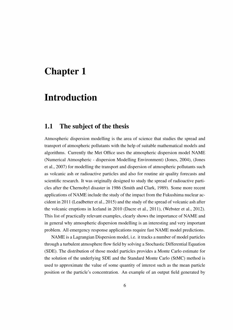
NAME is a Lagrangian Dispersion model, i.e. it tracks a number of model particlesthrough a turbulent atmosphere flow field by solving a Stochastic Differential Equation(SDE). The distribution of those model particles provides a Monte Carlo estimate forthe solution of the underlying SDE and the Standard Monte Carlo (StMC) method isused to approximate the value of some quantity of interest such as the mean particleposition or the particle’s concentration. An example of an output field generated by

6

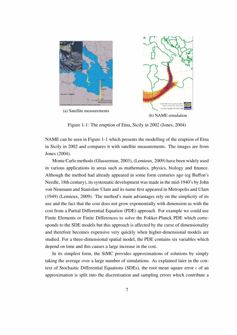
(a) Satellite measurements(b) NAME simulation

Figure 1-1: The eruption of Etna, Sicily in 2002 (Jones, 2004)

NAME can be seen in Figure 1-1 which presents the modelling of the eruption of Etnain Sicily in 2002 and compares it with satellite measurements. The images are fromJones (2004).

Monte Carlo methods (Glasserman, 2003), (Lemieux, 2009) have been widely usedin various applications in areas such as mathematics, physics, biology and finance.Although the method had already appeared in some form centuries ago (eg Buffon’sNeedle, 18th century), its systematic development was made in the mid-1940’s by Johnvon Neumann and Stanislaw Ulam and its name first appeared in Metropolis and Ulam(1949) (Lemieux, 2009). The method’s main advantages rely on the simplicity of itsuse and the fact that the cost does not grow exponentially with dimension as with thecost from a Partial Differential Equation (PDE) approach. For example we could useFinite Elements or Finite Differences to solve the Fokker-Planck PDE which corre-sponds to the SDE models but this approach is affected by the curse of dimensionalityand therefore becomes expensive very quickly when higher-dimensional models arestudied. For a three-dimensional spatial model, the PDE contains six variables whichdepend on time and this causes a large increase in the cost.

In its simplest form, the StMC provides approximations of solutions by simplytaking the average over a large number of simulations. As explained later in the con-text of Stochastic Differential Equations (SDEs), the root mean square error ε of anapproximation is split into the discretisation and sampling errors which contribute a

7

factor of ε−1 and ε−2 to the cost respectively. The total cost then has an asymptoticorder of ε−1 · ε−2 = ε−3 which becomes very large as ε decreases. In the literature,there are plenty of variance reduction techniques for example antithetic variables, con-trol variates and importance sampling (Glasserman, 2003), (Lemieux, 2009) which canreduce the cost of the method but without improving the asymptotic cost rate. In or-der to reduce the cost rate, we consider the Multilevel Monte Carlo (MLMC) method(Heinrich, 2001), (Giles, 2008) and its application to models used by the Met Office inatmospheric dispersion modelling.

Although for a low accuracy the StMC method can be fast enough, by increas-ing the accuracy it becomes very expensive and slow to run since the cost rate hasan asymptotic order of ε−3. Therefore, a more efficient method is required. TheMLMC method has been successfully applied in various areas such as mathematicalfinance (Giles, 2008), (Giles and Szpruch, 2012), partial differential equations withrandom coefficients (Cliffe et al., 2011) and uncertainty quantification in subsurfaceflows (Graham et al., 2015). The method showed its great potential of reducing theasymptotic order of the cost to ε−2 which makes it extremely important in many appli-cations. In particular, it can be very important to the Met Office since in an emergencyresponce situation, like for example a volcano eruption, it is necessary to produce fastand accurate predictions.

One of the key properties that lead to the cost rate reduction is the fact that MLMCconstructs a hierarchy of levels with larger timestep sizes and also computes estimatesof the differences between two estimators which have a smaller variance. Then, undercertain conditions, it can reduce the number of samples required to achieve a certaintolerance ε on the root mean square error and also shift the cost on the coarsest levelswhich are cheaper to compute since they use a larger timestep. In all methods that westudied, the bias of the SDE timestepping methods depends linearly on the timestepsize h, i.e. bias = C · h and the total cost is affected by the constant of proportionalityC. At the Met Office they currently use the Symplectic Euler timestepping methodso it becomes important to study more advanced methods which have a smaller biasconstant and therefore reduce the total cost.

In this thesis we study atmospheric dispersion models used by the Met Office whichdescribe the evolution of the particle’s position X(t) and particle’s turbulent velocitycomponent U(t) in the atmosphere. These models are given in d spatial dimensions

8

and have the general SDE form

dU(t) = −Λ (X(t)) U(t)dt−∇XV (X(t),U(t)) dt+ Σ (X(t)) dW(t), (1.1)

dX(t) = (U(t) + v (X(t), t)) dt, (1.2)

where X(t),U(t),v (X(t), t) ∈ Rd, V (X(t),U(t)) ∈ R, Λ (X(t)) and Σ (X(t)) arediagonal d×d matrices and W(t) is a d-dimensional Brownian motion (see Definition2.1). The notation ∇X means that we take the gradient vector only with respect to thevariable X. v (X(t), t) is the background velocity field, Λ (X(t)) contains velocitymemory terms, ∇XV (X(t),U(t)) guarantees the well-mixed condition (Thomson,1987) and Σ (X(t)) is the stochastic component.

The functions Λ (X(t)), V (X(t),U(t)), Σ (X(t)) and v (X(t), t) depend on thevalue of d and we will consider separately the three cases when d = 1, 2, 3. Whend = 1 the model will describe one-dimensional vertical dispersion, when d = 2 itwill describe a two-dimensional horizontal dispersion and when d = 3 it will describea three-dimensional dispersion that combines the vertical and horizontal structures ofthe first two cases. When d = 1 and d = 3 we assume that the motion of the particlesis constrained to a boundary layer of fixed height and as we describe later, some ofthe SDE coefficients in (1.1) and (1.2) will have singularities at the boundary points.Note that the boundary layer is the part of the atmosphere where turbulence plays asignificant role and hence the SDE which models this by a random term is applicable.

The main subject of the thesis is the implementation and theoretical analysis ofthe MLMC method to produce numerical approximations of the above model withan improved asymptotic rate of the order ε−2 as discussed above. For this, varioustimestepping methods must be explored that will enable us to discretise our models,reduce the total cost (by reducing the constant in the cost rates) and deal with anysingularities present in the SDE coefficients in order to produce particle trajectories.In addition to specifying the particles’ initial position and velocity it is necessary toadd suitable boundary conditions at the bottom and top of the boundary layer in theone- and three-dimensional setups. Since the particle trajectories themselves are notdirectly measurable, we are interested in approximating the value of E [φ(X(t))] forsome quantity of interest φ : Rd → R that describes a physical property. The quan-tity of interest φ can be simple and continuous, like for example the identity functionwhich gives the mean particle position but it can also be discontinous, like the indica-

9

tor function which gives the particle concentration. The latter can be used to measurethe volcanic ash present in certain regions of the atmosphere after a volcanic eruptionwhich is very important for air travelling.

Monte Carlo and timestepping methods are analysed both numerically and theo-retically. With the design of more efficient algorithms we compare the performance ofStandard and Multilevel Monte Carlo and apply alternative timestepping methods withhigher stability and study possible improvements. With suitable assumptions we studythe problem theoretically which will help in the improvement of the current algorithmsused by the Met Office by identifying the conditions under which our methods performbetter. In Section 1.2 we give a more detailed description of the aims and challengesof this thesis.

1.2 The aims of the thesis

The central aim of this thesis is the design of a Monte Carlo algorithm and more ad-vanced timestepping methods for SDEs in atmospheric dispersion modelling that willimprove the StMC-Symplectic Euler combination currently used by the Met Office. Inparticular, we are interested in implementing the MLMC method that will help us toimprove the asymptotic cost rate from ε−3 to ε−2. The overall cost, i.e. the constant inthe above cost rates, depends on the timestepping method and reducing this constantis also very important especially in physical applications which usually do not requirea small ε. To achieve this goal several difficulties need to be overcome.

Firstly, some of the coefficients in the SDE equations (1.1) and (1.2) have singular-ities at the end points of our boundary layer which can lead to severe limitations on thetimestep size and limit the use of MLMC. To make sure that our timestepping methodsremain stable we must deal with these singularities by either removing them with thehelp of some regularisation or by implementing more advanced methods which are lessaffected by them. In addition, our choice of timestepping methods must be justifiedby theoretical results which show that the SDE approximations converge to the exactsolution.

Next, we study under which conditions the MLMC method gives the improved costrate of ε−2 since this is not always the case. Our approach is the theoretical applica-tion of the complexity theorem (Giles, 2008) which requires the correct coupling ofrandom variables on the coarse levels. Each timestepping method requires a different

10

coupling treatment and this application can be supported by both numerical and theo-retical results where this is possible. For the theoretical application we use modifiedequations analysis (Shardlow, 2006), (Zygalakis, 2011), (Muller et al., 2015) which isan alternative approach to traditional strong approximation results.

Another challenge is the correct treatment of the boundary conditions at the topand bottom of the atmospheric boundary layer. In this thesis we consider simple elas-tic reflection. As we will see later if the random variables on subsequent levels are notcoupled correctly to account for reflection, then the MLMC variance increases and vi-olates one of the conditions in the complexity theorem (Giles, 2008) which is requiredto achieve the optimal ε−2 cost rate. Therefore, we need to develop an algorithm thatcontains the proper coupling of random variables when the particles are reflected.

Also, we need to be careful that our quantity of interest does not increase the vari-ance of the methods. One of the most important quantities considered in this thesisis the indicator function which gives an approximation of the particle concentration.The indicator function however is not continuous which causes an increase in the vari-ance and slows down the MLMC method. Therefore, it is important to find a suitablesmooth approximation that will reduce the variance and at the same time allow us tominimise any extra approximation errors.

All the above topics are first studied for a one-dimensional spatial model for verti-cal dispersion, i.e. equations (1.1) and (1.2) with d = 1 and also v(X(t), t) = 0. Later,higher dimensional models are explored where we also study the effect of a non-zerobackground velocity field v(X(t), t). In particular, we study a two-dimensional modelfor horizontal dispersion and a three-dimensional model that combines the first two.

Finally, based on the outcome of this thesis the methods that we study can then beimplemented in the Met Office’s NAME dispersion model. The ultimate goal is to useMLMC and the new timestepping methods to improve the performance of the NAMEmodel. This is important for many reasons like for example providing faster and moreaccurate results in emergency responce situations (eg volcano eruptions).

1.3 The main achievements

The main achievements of this thesis are:

(i) Successfully implemented MLMC in one-dimensional atmospheric dispersionmodelling and produced numerical results which clearly show the efficiency of

11

the MLMC over the StMC method for an inhomogeneous turbulence model, es-pecially for small tolerances. The results were produced using the C++ codeinitially developed for the paper Muller et al. (2015) and which we later enrichedfor the purposes of this thesis.

(ii) Studied possible improvements on the performance of Monte Carlo from morestable and accurate timestepping methods. In particular, we compare the Sym-plectic Euler method currently used by the Met Office with two improved meth-ods, the Geometric Langevin (Bou-Rabee and Owhadi, 2010) and BAOAB (Leimkuh-ler and Matthews, 2015) which are based on an SDE splitting approach. We ob-served that timestepping methods based on a splitting approach can reduce theStMC cost when applied to one-dimensional models with varying turbulence pro-files. As a result, their combination with StMC can be a better choice for largetolerance errors.

(iii) Developed and implemented a new algorithm for the treatment of reflective bound-ary conditions which preserves the quadratic variance decay of the MLMC method(Katsiolides et al., 2018). The new method is based on extending the initial modelwith reflection to a model without reflection which results in the correct couplingof random variables in the MLMC coarse steps.

(iv) Applied the smoothing polynomial technique as in Giles et al. (2015) to dealwith the discontinuity of the indicator function in the concentration problem.With this approximation we improve the MLMC variance rates and therefore theperformance.

(v) Proved existence and uniqueness of a regular solution of the inhomogeneous one-dimensional model using a Lyapunov function and the theory in Khasminskii(2011). Using the same Lyapunov function and the theory from Milstein andTretyakov (2005) we also show that under some assumptions our timesteppingmethods converge weakly.

(vi) Proved theoretically that the complexity theorem (Giles, 2008) holds for the one-dimensional models with suitable regularisation. For a simplified model rep-resenting homogeneous turbulence we apply a direct approach based on strongapproximation results. For our inhomogeneous model we apply a method based

12

on the theory of modified equations (Shardlow, 2006), (Zygalakis, 2011), (Mulleret al., 2015) which provides an alternative approach to the strong approximationresults.

(vii) Implemented an adaptive MLMC (Giles et al., 2016) algorithm for one-dimensionalmodels and observed some small improvements for the Symplectic Euler method.

(viii) Implemented StMC and MLMC for two- and three-dimensional models. Weobserved that for higher dimensional models the MLMC method improves theasymptotic cost rate when compared to StMC. Also, we demonstrated that insome cases the BAOAB method can reduce the overall cost of StMC.

1.4 The structure of the thesis

In Chapter 2 we introduce our one-dimensional models and describe the physical in-terpretation of the basic variables. We describe the model scales by using dimensionalanalysis, define the boundary conditions and discuss how we deal with the singularitiesin the turbulence profiles present in the models. Then, we talk about the quantities ofinterest that we are going to approximate, compute the systems invariant measure anddiscuss some relations with molecular dynamics.

In Chapter 3 we present the timestepping methods that we use to discretise theone-dimensional models and define the Standard and Multilevel Monte Carlo methodsin the context of SDEs. We review the Symplectic Euler method currently used bythe Met Office and also define two more advanced methods, the Geometric Langevinand BAOAB which are based on SDE splitting methods. We then describe how wemeasure the Monte Carlo approximation errors and the strategy we follow in order toachieve a certain error tolerance. Also, we derive a theoretical bound for the StMCcost rate as a function of the error tolerance and review the complexity theorem (Giles,2008) which explains when the MLMC method has a better cost rate when comparedto StMC.

In Chapter 4 we present some theoretical results about the one-dimensional models.We begin by proving that our basic inhomogeneous model has a unique solution by us-ing a Lyapunov function and the theory in Khasminskii (2011). We then talk about theconvergence of our timestepping methods and using the same Lyapunov function with

13

the theory from Milstein and Tretyakov (2005) we show that under certain conditionsthey are all weakly convergent to the exact solution.

In Chapter 5 we study the theoretical application of the complexity theorem (Giles,2008) to the particular one-dimensional models in atmospheric dispersion modelling.In Section 5.1 we consider a simplified model and present a direct approach based onstrong approximation results. In Section 5.2 we present a new algorithm for the cor-rect treatment of reflective boundary conditions (Katsiolides et al., 2018). The basicidea is to extend the initial model to a problem without boundary conditions and countthe number of reflections which then gives the correct coupling of random variablesin the MLMC coarse levels. In Section 5.3 we study the conditions under which thecomplexity theorem holds for our basic inhomogeneous model using an alternativeapproach based on modified equations analysis (Shardlow, 2006), (Zygalakis, 2011),(Muller et al., 2015). Lastly, in Section 5.4 we describe how we deal with the discon-tinuity of the indicator function in the concentration problem by using the smoothingpoynomial technique from Giles et al. (2015).

In Chapter 6 we present several numerical experiments for the one-dimensionalmodels to compare the efficiency of Standard and Multilevel Monte Carlo with ourtimestepping methods. We study the mean particle position, concentration and densityfunction; all results and conclusions in this section have been published in Katsiolideset al. (2018). In all the experiments we use a uniform timestep size except from thelast part of the chapter where we consider adaptive timestepping.

In Chapter 7 we study higher-dimensional models. We construct a realistic back-ground velocity field (i.e. the function v(Xt, t)) in equation (1.2)) with the correct en-ergy spectrum (Nastrom and Gage, 1985) and a realistic wind-shear due to the Ekmanspiral (Holton, 2004). We then discuss the corresponding model scales, the particlespread plots and finally present numerical results for two- and three-dimensional mod-els. For the numerical results we consider only one quantity of interest, the particleconcentration.

In the Conclusion, we summarise all the achievements, suggest some ideas forfurther research and finally in the Appendix we present the technical details of someof the results of this thesis.

14

Chapter 2

Atmospheric Dispersion Modelling

Atmospheric dispersion modelling studies the spread and transport of atmospheric pol-lutants and is important at the Met Office in many areas such as emergency responsesituations (volcano eruptions, nuclear accidents, smoke from large fires etc) and rou-tine forecasting applications. To model the dispersion, the three dimensional total ve-locity field u(X, t), which depends on both the spatial coordinate X and time t, is firstsplit into two components. The first component corresponds to the large-scale flowv(X, t) which is a deterministic velocity field and is given from the Met Office’s fore-cast model. The second component corresponds to the unresolved turbulence U(X, t)

which can be modelled by a stochastic velocity field. Combining these two quantitieswe can then write

u(X, t) = v(X, t) + U(X, t). (2.1)

The velocity field v(X, t) has the property that

v(X, t) = 〈u(X, t)〉, (2.2)

where 〈·〉 denotes the ensemble average. The ensemble average of U(X, t) is zerosince as we see later, the turbulence is assumed to be Gaussian with mean zero. FromGeorge (2009) the ensemble average of an observable quantity A which depends onthe particle position and velocity, is defined by

〈A〉 = limN→∞

1

N

N∑n=1

a(n), (2.3)

15

where a(n) is the nth realisation ofA, i.e. the value ofA obtained at the nth independentand identical repetition of the experiment.

At the Met Office, particle dispersion is studied by using the NAME LagrangianDispersion model. Lagrangian dispersion models describe the transport of a passivetracer particle in a turbulent velocity field in the form of an SDE. For a given particle,the Lagrangian velocity is the velocity at a given time t and each particle follows themean flow v(X, t) to which we then add a random velocity component U(t). Morespecifically, U(t) denotes the turbulent component of the Lagrangian velocity and atequilibrium, i.e. after a large travel time, it agrees in distribution with the turbulentfield U(X, t) for particles which pass through point X at time t (Katsiolides et al.,2018). A general SDE in d spatial dimensions for a Lagrangian dispersion model(later simply called d-dimensional) can be written as

dU(t) = −Λ(X(t))U(t)dt−∇XV (X(t),U(t))dt+ Σ(X(t))dW(t), (2.4)

dX(t) = (U(t) + v(X(t), t))dt, (2.5)

where X(t),U(t),v(X(t), t) ∈ Rd, V (X(t),U(t)) ∈ R, Λ(X(t)) and Σ(X(t)) arediagonal d × d matrices and W(t) is a d-dimensional Brownian motion. Accordingto this model, the particles follow the mean velocity v(X(t), t), called backgroundvelocity, to which we add the random variable U(t) that represents turbulence. Wealso assume that the particles are independent, non-interacting and of unit mass. Thefollowing definition of Brownian motion can be found in Lemieux (2009).

Definition 2.1. A standard one-dimensional Brownian motion is a continuous-time

stochastic process W (t), t ≥ 0 with the following properties:

1. W(0) = 0.

2. The increments over disjoint intervals are independent, i.e. for r < s < t < u

we have that W (u)−W (t) and W (s)−W (r) are independent.

3. The increments are stationary, i.e. for any r, s, t > 0 we have that W (r + t) −W (r) and W (s + t) −W (s) have the same probability density function, which

is normal with mean 0 and variance t.

A d-dimensional Brownian motion W(t) is a vector of d independent Brownian mo-

tions W (t).

16

Note that we could also consider a deterministic model by solving the correspond-ing Fokker-Planck Partial Differential Equation (also called Kolmogorov’s ForwardEquation) which is equivalent to solving the SDE (Øksendal, 2003). For the SDEs(2.4) and (2.5) it is given by

∂ρ

∂t=−

d∑i=1

[∂

∂Xi

[(Ui + vi(X, t)) ρ] +∂

∂Ui

[(−Λii(X)Ui −

∂V

∂Xi

(X,U)

)ρ

]]

+1

2

d∑i=1

∂2

∂U2i

[(Σii(X))2 ρ

], (2.6)

where ρ(X,U, t) is the probability density of the particles in the phase space definedby their position and velocity. The index i denotes the ith component of the corre-sponding variable. We could then use Finite Elements or Finite Differences to approx-imate the solution. This approach however is affected by the curse of dimensionalitysince we have 2d number of variables which depend on time and this gives a furtheradvantage to the Monte Carlo method whose cost does not grow exponentially withdimension. Here we consider only Monte Carlo methods applied to SDEs and thecomparison with the Fokker-Planck approach can be a topic for future research.

For simplicity, and since in the atmosphere the strongest variations usually occurin the vertical direction, we firstly consider one-dimensional models which means thatwe study equations (2.4) and (2.5) with d = 1. These models describe vertical dis-persion and we also set v(X, t) = 0 (where X is the vertical coordinate) since thevertical background velocities are much smaller than the horizontal velocities and canbe neglected. Later, in Chapter 7 we present the generalisation to higher dimensions.

This chapter is structured as follows. Firstly, we introduce our basic one-dimen-sional model for inhomogeneous turbulence and describe the equations’ coefficientsand variables. Then, we introduce a simplified version of the first model which de-scribes dispersion in a homogeneous turbulence field. Next, we describe the modelscales by using dimensional analysis, discuss how we deal with the singularities presentin the model and present our choice of boundary conditions. Finally, we briefly dis-cuss the quantities of interest that we are going to approximate and also describe someconnections to molecular dynamics. Here we also compute the system’s invariant mea-sure.

17

2.1 The one-dimensional Inhomogeneous turbulencemodel

Our basic one-dimensional model for vertical dispersion assumes stationary (indepen-dent of time) and inhomogeneous (dependent of position) turbulence and is given bythe following SDE

dU(t) = −λ(X(t))U(t)dt− ∂V

∂X(X(t), U(t))dt+ σ(X(t))dW (t), (2.7)

dX(t) = U(t)dt. (2.8)

In this equation, t is the time, U(t) is the Lagrangian vertical velocity fluctuation dueto turbulence, X(t) is the vertical position and W (t) is a Brownian motion. The co-efficients λ(X), ∂V

∂X(X,U) and σ(X) are given in terms of the two functions σU(X),

τ(X) and are related by

λ(X) =1

τ(X), σ(X) =

√2σ2

U(X)

τ(X), (2.9)

∂V

∂X(X,U) = −1

2

[1 +

(U

σU(X)

)2]∂σ2

U

∂X(X). (2.10)

With this notation, the function V (X,U) can also be written as

V (X,U) ≡ −1

2

[σ2U(X) + U2 log

(σ2U(X)/σ2

U(Xref))], (2.11)

where Xref is a fixed reference height. σ2U(X) is the variance of the turbulent com-

ponent of the background velocity field and τ(X) is the Lagrangian local velocitydecorrelation timescale. The form of these functions will be discussed in Section 2.2.Although the velocityU(t) depends on time we call the model stationary because τ(X)

and σU(X) are independent of t. Similarly, we call the model inhomogeneous becauseτ(X) and σU(X) depend onX . We assume that the motion of the particles is restrictedto a boundary layer of height H , i.e. their vertical position can only vary between 0

and H (see also Figure 2-2).Next, we need to specify suitable initial conditions (X(0), U(0)) which can either

be deterministic or stochastic depending on the problem. For the one-dimensional

18

model we assume that both quantities are deterministic. For higher-dimensional mod-els however, and since the background velocity is non-zero we assume that the initialvelocity adapts to the ambient velocity of the flow when the particles are released.Practically this means that the initial position is still deterministic but the initial veloc-ity is random with each component independent and normally distributed with meanzero and variance σ2

U(X(0)) (for higher-dimensional models this function can be dif-ferent in each direction).

Equation (2.7) was derived in Thomson (1987) where the author presents severalcriteria for the selection of these stochastic Lagrangian models. These criteria are alsoreviewed in Rodean (1996). One of the most important, is the well-mixed condition(Thomson, 1987) that gives rise to the coefficient ∂V

∂X(X(t), U(t)) and requires that

particles which are initially uniformly mixed to stay uniformly mixed. In mathemati-cal terms this means that the stationary distribution of the particle density ρ(X,U) of(X(t), U(t)) has two basic properties. The first property is that the marginal distribu-tion of X (i.e. ρ(x) =

∫∞−∞ ρ(x, u)du) is uniform in space and the second property is

that conditioned on X we have that ρ(u|x = X) has the same distribution as the unre-solved turbulence U(X, t) which is assumed to be Gaussian (Katsiolides et al., 2018).In Lemma 2.3 we verify that this is indeed the case by showing that the stationarydistribution is given by

ρ(X,U) =1√

2πσU(X)exp

(− U2

2σ2U(X)

), (2.12)

which also requires that the function V (X,U) has the form given by equation (2.11).Other criteria include the correct behaviour of the small-time velocity distribution ofparticles from a point source and the consistency of the forward and reverse dispersionformulations. However, as it is proved in Thomson (1987) these criteria follow fromthe well-mixed condition.

2.1.1 Simplification to homogeneous turbulence

The main numerical results that we present for the one-dimensional case are for theinhomogeneous model that we have just described. However, for global dispersionapplications and for long time scales, a simplified form of equation (2.7) can be usedin the approximations. This simplified model is obtained by assuming that τ(X) and

19

σU(X) in equation (2.7) are constants which gives

dU(t) = −λU(t)dt+ σdW (t), (2.13)

dX(t) = U(t)dt, (2.14)

where λ = 1τ

and σ =

√2σ2U

τ. Since τ and σU are now independent of X the model

describes homogeneous turbulence. A review of its derivation can be found in Rodean(1996).

All variables are as in the inhomogeneous model but now τ is equal to the timescalefor the Lagrangian velocity autocorrelation of U(t). In Taylor (1921) cited in Rodean(1996) the following equations were introduced for the timescale τ when the turbu-lence is homogeneous:

τ =

∫ ∞t0

R(t− t0)dt, (2.15)

withR(t− t0) =

〈U(t)U(t0)〉〈U2(t0)〉

, (2.16)

where t0 is a reference time and 〈·〉 denotes the ensemble average. In Taylor (1921) itis noted that the limiting form of a series expansion for the correlation coefficient R inequation (2.16) gives

R(t− t0) = e−(t−t0)/τ , (2.17)

and therefore we can see that the autocorrelation decays exponentially with a charac-teristic timescale τ . Equation (2.17) can also be verified using the solution of equation(2.13) (See Appendix A.1).

The only results that we present for the homogeneous model are in Section 5.1where we prove theoretically that the MLMC method performs with a better cost rate.Note that the simplified model has an analytic solution that we compute in AppendixA.2 where we also present some analysis of the spread of the particles.

2.1.2 Model scales and dimensional analysis

Before computing any numerical approximation involving our SDE models it is nec-essary to non-dimensionalise all the parameters since our code’s input parameter filecannot contain any physical units. This dimensional analysis allows the physical inter-pretation of the numerical results by introducing suitable model scales.

20

For a physical quantity α we consider a reference scale αref and write

α = αrefα, (2.18)

where α is the corresponding dimensionless parameter. In particular, for our model weconsider a reference length X ref, a reference speed U ref, a reference time T ref and write

X(t) = X refX(t), U(t) = U refU(t), t = T reft, (2.19)

where X(t), U(t) and t are the corresponding dimensionless quantities. Substitutingin equation (2.8) gives

X refdX(t) = U refT refU(t)dt, (2.20)

so the reference variables are simplified and give the same equation as with the physicalparameters provided

X ref = U refT ref. (2.21)

In the following, we drop the hats from these variables and use dimensionless quan-tities in the equations, under the assumption that they measure the physical quantitiesin the units defined by X ref, U ref and T ref. We choose X ref = 1000m (since our bound-ary layer’s height is 1km) and U ref = 1m/s which gives T ref = 1000s = 162

3min.

As an example of how we use these scales in practise suppose that we are interestedin releasing particles from an initial height of 50m with an initial velocity of 0.1m/s.This simply means that we set X(0) = 0.05 and U(0) = 0.1.

2.2 The functions σU(X) and τ (X)

As discussed in Section 2.1 our inhomogeneous model contains the functions σU(X)

and τ(X) and their exact form depends on the atmospheric conditions of the boundarylayer which is assumed to be of height H . In Webster et al. (2003) several profilesfor σU(X) and τ(X) are proposed which take into account stability conditions in theatmosphere. As a representative choice, we use the following form of σU(X) as inWebster et al. (2003) for neutral and stable conditions

σU(X) = κσu∗(

1− X

H

) 34

, X ∈ (0, H), (2.22)

21

where u∗ is the friction velocity and κσ some dimensionless constant. For τ(X) weuse

τ(X) = κτX

σU(X), X ∈ (0, H), (2.23)

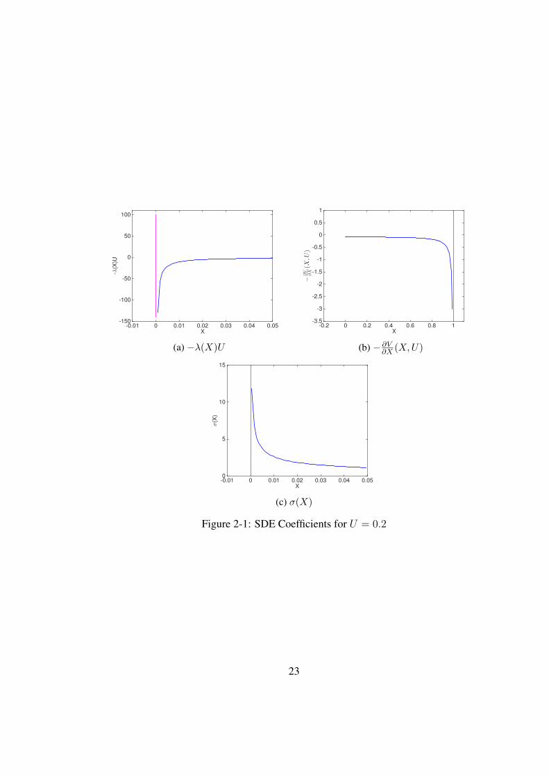
for some dimensionless constant κτ which agrees with Wilson et al. (2009) wherethe expression τ(X) ≈ 0.5X/σU is derived for a neutrally stable surface layer andhorizontally homogeneous turbulence. Although there is some uncertainty in the exactform of these profiles, exploring more cases is beyond the scope of this thesis so weonly focus on the above representative case. In our numerical experiments we useκσ = 1.3, κτ = 0.5, u∗ = 0.2 and H = 1 as in Cook (2013).

In equations (2.22) and (2.23) we can easily observe that σU(X) and τ(X) havesingularities or they are zero at the boundaries X = 0 and X = H and as a result someof the SDE coefficients in (2.7) diverge near the boundaries. In Figure 2-1 we plot theSDE coefficients −λ(X)U , − ∂V

∂X(X,U) and σ(X) and we can see that as X tends to

zero or H(= 1) some of the functions tend to infinity.With these singularities it now becomes hard to simulate any trajectories and es-

tablish well-posedness since when the particles reach the boundaries we obtain infinitevalues which make some timestepping methods unstable. In order to deal with thesingularities we regularise the functions τ(X) and σU(X) by setting them to constantvalues below a height εreg and above a height H − εreg. More specifically, we use thesame regularisation as the Met Office by setting

τ(X) = τ(εreg), σU(X) = σU(εreg) if X < εreg, (2.24)

τ(X) = τ(H − εreg), σU(X) = σU(H − εreg) if X > H − εreg, (2.25)

where 0 < εreg H is some small regularisation constant. Consequently, the func-tions τ(X) and σU(X) can never be evaluated at the points X = 0 or X = H whichcreate the singularities and they are bounded with τ(εreg) ≤ τ(X) ≤ τ(H − εreg) andσU(H − εreg) ≤ σU(X) ≤ σU(εreg). Currently at the Met Office τ(X) is kept constantbelow the height at which the physical value of τ(X) equals 20 sec. Using this prop-erty and the parameter values of τ(X) given above gives approximately εreg = 0.01

which corresponds to a physical height of 10m. The effect of εreg on the numericalresults is studied in Section 6.4.1.

22

X-0.01 0 0.01 0.02 0.03 0.04 0.05

-λ(X

)U

-150

-100

-50

0

50

100

(a) −λ(X)U

X

-0.2 0 0.2 0.4 0.6 0.8 1

−

∂V

∂X(X

,U)

-3.5

-3

-2.5

-2

-1.5

-1

-0.5

0

0.5

1

(b) − ∂V∂X (X,U)

X-0.01 0 0.01 0.02 0.03 0.04 0.05

σ(X

)

0

5

10

15

(c) σ(X)

Figure 2-1: SDE Coefficients for U = 0.2

23

H Boundary Layer

Free Atmosphere

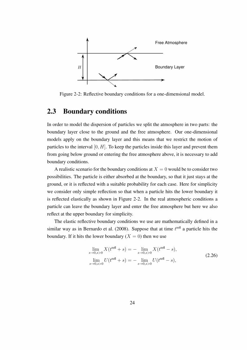
Figure 2-2: Reflective boundary conditions for a one-dimensional model.

2.3 Boundary conditions

In order to model the dispersion of particles we split the atmosphere in two parts: theboundary layer close to the ground and the free atmosphere. Our one-dimensionalmodels apply on the boundary layer and this means that we restrict the motion ofparticles to the interval [0, H]. To keep the particles inside this layer and prevent themfrom going below ground or entering the free atmosphere above, it is necessary to addboundary conditions.

A realistic scenario for the boundary conditions atX = 0 would be to consider twopossibilities. The particle is either absorbed at the boundary, so that it just stays at theground, or it is reflected with a suitable probability for each case. Here for simplicitywe consider only simple reflection so that when a particle hits the lower boundary itis reflected elastically as shown in Figure 2-2. In the real atmospheric conditions aparticle can leave the boundary layer and enter the free atmosphere but here we alsoreflect at the upper boundary for simplicity.

The elastic reflective boundary conditions we use are mathematically defined in asimilar way as in Bernardo et al. (2008). Suppose that at time trefl a particle hits theboundary. If it hits the lower boundary (X = 0) then we use

lims→0,s>0

X(trefl + s) = − lims→0,s>0

X(trefl − s),

lims→0,s>0

U(trefl + s) = − lims→0,s>0

U(trefl − s),(2.26)

24

and if it hits the upper boundary (X = H) we use

lims→0,s>0

X(trefl + s) = 2H − lims→0,s>0

X(trefl − s),

lims→0,s>0

U(trefl + s) = − lims→0,s>0

U(trefl − s).(2.27)

Note that the condition on X(t) is unnecessary as it follows from continuity, but westill include it because it will be helpful in the implementation of the boundary condi-tions in the discretisation methods discussed in section 3.1. More information aboutboundary conditions can be found in Rodean (1996) where the author presents a shortreview of various approaches found in the literature and how they interact with someof the model’s quantities like for example the velocity decorrelation timescale τ(X).

Note that at any point in time the total mass is obtained by summing the massesof all model particles. Since in our model the mass of an individual particle does notchange over time, mass conservation follows trivially if no trajectories are terminatedand this is the case for the non-absorptive reflective boundary conditions consideredhere.

In Section 5.2 we discuss in more detail the effect of the boundary conditions inthe performance of the MLMC method. As we will see, when reflection is not treatedcorrectly it reduces the efficiency of the MLMC method and we will provide a newtechnique for the correct coupling of random variables in the presence of reflectiveboundary conditions which does not reduce the performance. This new technique willbe based on extending the domain of X to the whole real line and make the problemequivalent to the one without boundary conditions.

Finally, we note that with the choice of reflective boundary conditions and undersome assumptions on the functions σU(X) and τ(X) it is possible to show existenceand uniqueness of a solution to the inhomogeneous model. In Section 4.1 we includethe details of the proof which is based on the existence of a Lyapunov function and thetheory from Khasminskii (2011).

2.4 Quantities of interest

While the numerical solution of the SDE will give a set of paths, our main interest is toapproximate the mean value of some functional φ of the path (X(t), U(t)) which wecall the quantity of interest. In particular, we study the mean particle position E[X(T )]

25

and the concentration E[1[a,b](X(T ))

]for some T > 0 and a, b ∈ R. The indicator

function in the concentration problem is defined by

1[a,b](x) =

1 if x ∈ [a, b],

0 otherwise.

We first study the mean particle position because it is the simplest case to consider andthen we study the concentration which is very important in atmospheric dispersion andof particular interest to the Met Office. As we will see later in Section 6.3, we can usea vector of indicator functions to construct a piecewise constant approximation to theconcentration field at any given time T . For example, this would allow predicting theconcentration of volcanic ash that a plane may encounter on different flight levels.

2.5 Relations with molecular dynamics

To put our work into a wider context, we now discuss some relations between ourone-dimensional models and other areas of modelling and in particular molecular dy-namics. The SDE equations (2.4) and (2.5) have the form of a well-known class ofequations called the Langevin equations, which are also used for modelling in molecu-lar dynamics. If we denote by X and U the particles’ position and momentum vectorsrespectively then the simplified form of SDEs

dU(t) = −λU(t)dt−∇G(X(t))dt+ σdW(t), (2.28)

dX(t) = U(t)dt, (2.29)

for some function G, constants λ and σ and Brownian motion W(t) (see Definition2.1) are used to model a system of particles in a heat bath (Leimkuhler and Matthews,2015). The dimension of X and U is now equal to the number of particles. The onlyinteraction between the system of particles and the heat bath is the exchange of energyand when equilibrium is reached, the equilibrium distribution is given by

ρ(X,U) = Z−1 exp

(−2λ

σ2

(1

2UTU +G(X)

)), (2.30)

26

where Z is a normalisation constant. Equation (2.30) is called Gibbs canonical distri-bution. The constants λ and σ are related with the system’s temperature T with theequation

κBT =σ2

2λ, (2.31)

where κB is Boltzmann’s constant (Leimkuhler and Matthews, 2015).In our inhomogeneous model equation (2.7), the derivative on the right hand side

also depends on the velocity and this is due to the well-mixed condition (Thomson,1987), (Rodean, 1996). The Gibbs canonical distribution equation (2.30) can motivatethe choice of the invariant measure of our inhomogeneous model equations (2.7) and(2.8).

Definition 2.2. The function ρ(X,U, t) is called an invariant measure or equilibrium

distribution for the SDEs (2.7) and (2.8) if it satisfies the Fokker-Planck equation (2.6)with ∂ρ

∂t= 0 (Leimkuhler and Matthews, 2015).

We give this measure in the following lemma.

Lemma 2.3. An invariant measure of the system of equations (2.7) and (2.8) without

boundary conditions is given by

ρ(X,U) =1√

2πσU(X)exp

(− U2

2σ2U(X)

), (2.32)

where σU(X) is assumed to be sufficiently smooth.

Proof . From Definition 2.2 it is enough to show that equation (2.32) satisfies thecorresponding Fokker-Planck equation with ∂ρ

dt= 0.

Using (2.6), the Fokker-Planck equation is given by

∂ρ

dt= − ∂

∂u

[[− u

τ(x)+

1

2

[1 +

u2

σ2U(x)

]∂σ2

U(x)

∂x

]ρ

]− ∂

∂x(uρ)+

1

2

∂2

∂u2

[2σ2

U(x)

τ(x)ρ

],

where ρ(x, u, t) is the density of (X(t), U(t)) and simplifying gives

∂ρ

dt=

ρ

τ(x)+

u

τ(x)

∂ρ

∂u− σU(x)

∂σU(x)

dx

∂ρ

∂u− 2uρ

σU(x)

∂σU(x)

∂x− u2

σU(x)

∂σU(x)

∂x

∂ρ

∂u

− u∂ρ∂x

+σ2U(x)

τ(x)

∂2ρ

∂u2. (2.33)

27

Differentiating equation (2.32) gives

∂ρ

du= − uρ

σ2U(x)

,∂2ρ

du2= − ρ

σ2U(x)

+u2ρ

σ4U(x)

,∂ρ

dx= − ρ

σU(x)

∂σU(x)

∂x+

u2ρ

σ3U(x)

∂σU(x)

∂x,

and substituting in (2.33) we get∂ρ

dt= 0.

Lemma 2.3 completes our discussion about the well-mixed condition after we de-fined the inhomogeneous model in Section 2.1. As we can see from equation (2.32),the marginal distribution ofX , ρ(x) =

∫∞−∞ ρ(x, u)du = 1, is uniform in space and the

conditional distribution ρ(u|x = X) is Gaussian with mean zero and variance σ2U(X).

Lastly, from equation (2.31) we note that in the context of molecular dynamicsσ2U = σ2

2λ= κBT and therefore, σ2

U can be seen as the system’s “temperature”.However, the σ2

U that we are using in our one-dimensional models is not relatedto the air-temperature. It only describes measures of the fluctuation in the particlevelocity due to turbulence and it is computed using data based on observations ofvelocity variances (Webster et al., 2003). Also, molecular diffusion is negligible com-pared to turbulent diffusion and the reason is that Dmolecular = σ2

U,molecular · τmolecular

is much smaller than Dturbulence = σ2U,turbulence · τturbulence. The variable Dc where c =

molecular, turbulence is called the diffusion constant and after time T τc the parti-cles travel at a distance

√DcT by diffusion. Since Dmolecular is much smaller we can

then neglect molecular diffusion.

28

Chapter 3

Timestepping and Monte Carlomethods

Except for very special cases (such as the homogeneous turbulence model consideredin Section 2.1.1) it is not possible to solve an SDE exactly. Instead, usually two ap-proximations are made to obtain a numerical solution: (a) the total integration time issplit into a finite number of small intervals and (b) expectation values (in the compu-tation of quantities of interest) are replaced by Monte Carlo estimators. The stabilityand accuracy of both approximations need to be studied carefully.

In this chapter we define discrete timestepping methods and Standard and Multi-level Monte Carlo methods in the context of SDEs. Firstly, we present three timestep-ping methods called Symplectic Euler, Geometric Langevin and BAOAB which willenable us to produce particle trajectories of our SDE models. Then, we define MonteCarlo methods and describe how we measure the approximation errors. Also, we dis-cuss how we choose the timestep size and the number of samples in order to achieve aparticular tolerance on the total root mean square error. Finally, we compute the costrate of StMC and we include the complexity theorem (Giles, 2008) that describes theconditions which guarantee a better asymptotic cost rate for the MLMC method.

3.1 Timestepping methods

To discretise our inhomogeneous model SDEs (2.7) and (2.8) we use three explicittimestepping methods. These methods are also extensions to SDEs of symplectic

29

methods for Hamiltonian systems. This means that when they are applied in a Hamil-tonian system of Ordinary Differential Equations (ODEs) given by

dU

dt= −∂H

∂X,

dX

dt= +

∂H

∂U,

for some functionH(X,U) (called the Hamiltonian) they preserve the system’s Hamil-tonian dynamics. In a Hamiltonian system the total area of the flow is preserved andif a timestepping method does not change this property is called symplectic (Haireret al., 2006). The methods we use were chosen because the first one (Symplectic Eu-ler) is very popular in operational models due to its simplicity and is currently usedby the Met Office. The other two (Geometric Langevin, BAOAB) do not have anystability constraints on the timestep size as we discuss below (i.e. some restrictionon the timestep size to make sure that the numerical approximation does not becomelarge very quickly). More timestepping methods for SDEs, including the ones thatwe present here, can be found in Hairer et al. (2006), Kloeden and Platen (2011),Leimkuhler and Matthews (2015) and Muller et al. (2015). We define all timesteppingmethods in terms of the one-dimensional models and for higher dimensions we simplyapply the same method on each direction.

In our numerical experiments we are interested in finding an approximation of thesolution of the SDE models at time T so we integrate the SDE over the time interval[0, T ]. Discretising in time, this interval will then be split into M subintervals ofsize h = T/M and the exact solution (X(tn), U(tn)) is estimated at time tn = nh

for each n ∈ 0, . . . ,M. For each n the approximation is denoted by (Xn, Un) ≈(X(tn), U(tn)).

The first timestepping method is the Symplectic Euler method (see for exampleHairer et al. (2006)), currently used by the Met Office, and is given by

Un+1 = (1− λ(Xn)h)Un −∂V

∂X(Xn, Un)h+ σ(Xn)

√hξn, (3.1)

Xn+1 = Xn + Un+1h, (3.2)

where ξn ∼ Normal(0, 1) are independent and identically distributed (i.i.d.) Normalrandom variables. We observe that Xn+1 is computed using Un+1 and this makes the

30

method symplectic for Hamiltonian systems (i.e. when λ(x) = σ(x) = 0 and V inde-pendent of U ). Replacing Un+1 with Un in equation (3.2) gives the Euler Maruyamamethod (see for example Hairer et al. (2006)) which is not symplectic. The SymplecticEuler method is stable if the timestep size h satisfies |1− λ(Xn)h| < 1 which leadsto the constraint h < 2

λ(Xn). As a result, for the solution to be stable, for large λ(X)

we have to choose smaller timesteps which increase the computational time and cost.In particular, for the inhomogeneous model, λ(X) becomes large at the bottom of theboundary layer and this can lead to prohibitively tight bounds on the timestep size.

The other two timestepping methods, which do not have a stability issue are basedon a splitting approach (Leimkuhler and Reich, 2004), (Leimkuhler and Matthews,2015). For this, we write the SDE (2.7) in the form

dU(t) = dU (O)(t) + dU (B)(t), (3.3)

dX(t)

dt= 0, (3.4)

where

dU (O)(t) = −λ(X(t))U (O)(t)dt+ σ(X(t))dW (t), (3.5)

dU (B)(t) = −∂V∂X

(X(t), U (B)(t))dt. (3.6)

with the accompanying velocity equation

dX(t) = U(t)dt. (3.7)

Equations (3.5), (3.6) and (3.7) are discretised separately and one of the advantages ofthis method is that it may simplify a complicated problem by breaking it into a seriesof smaller and simpler problems. In addition, as we see below, the splitting methodsthat we consider have the very important property of not requiring any constraint onthe timestep size in order to be stable.

In particular, when discretising equations (3.5) and (3.6) we assume that X(t) isconstant in the interval [tn, tn+1) (and equals Xn) and therefore we can solve equation(3.5) as an exact Ornstein-Uhlenbeck process over a single step. This removes thestability constraint and also improves the performance of the Monte Carlo method asdemonstrated in Muller et al. (2015). As we will see, the term λ(Xn)h will appear as

31

a negative exponent to the exponential function and when λ(Xn) is large this expres-sion will simply vanish without creating any stability problems as with the SymplecticEuler method. As we will see in Chapter 6 these methods reduce the bias error of theapproximations. Following the notation from Leimkuhler and Matthews (2015) we re-fer to equation (3.5) as the O-update, to equation (3.6) as the B-update and to equation(3.7) as the A-update.

The first method based on this splitting is the Geometric Langevin method (Bou-Rabee and Owhadi, 2010) defined by

U?n+1 = e−λ(Xn)hUn + σ(Xn)αhξn, (3.8)

Un+1 = U?n+1 −

∂V

∂X(Xn, U

?n+1)h, (3.9)

Xn+1 = Xn + Un+1h, (3.10)

with αh =√

(1− e−2λ(Xn)h) /2λ(Xn) and ξn ∼ Normal(0, 1) i.i.d. The method wasintroduced in the context of MLMC in Muller et al. (2015) and referred to as “Sym-plectic Euler/Ornstein - Uhlenbeck Splitting Method”. The only difference in Mulleret al. (2015) is that the potential function V depends just on X . With the notation fromLeimkuhler and Matthews (2015) it can also be called OBA. This method was derivedby first solving the Ornstein-Uhlenbeck process equation (3.5) over a single step andthen by applying simple forward Euler steps on equations (3.6) and (3.7).

With this method there are no stability problems since when λ is large the exponen-tial function simply disappears without any constraints on the choice of the timestepsize. However, as we will see, when λ is large the multilevel variance increases andwe discuss this for the simplified model in Section 5.1.

Note that for the simplified model where λ and σU are constants, letting λ→∞ inequations (3.8) and (3.9) gives

Un+1 = σUξn. (3.11)

This expression is also obtained by discretising the exact solution from Appendix A.2.1and then letting λ → ∞. This property is clearly not true for the Symplectic Eulermethod since by letting λ→∞ in equation 3.1 we obtain an infinite value.

The third and last timestepping method, which is also based on a splitting approach,is the Symmetric Langevin Velocity-Verlet method (Leimkuhler and Matthews, 2015)

32

defined by

Un+ 12

= Un −∂V

∂X(Xn, Un)

h

2, (3.12)

Xn+ 12

= Xn + Un+ 12

h

2, (3.13)

U?n+ 1

2= e

−λ(Xn+ 1

2)hUn+ 1

2+ σ(Xn+ 1

2)αh(Xn+ 1

2)ξn, (3.14)

Xn+1 = Xn+ 12

+ U?n+ 1

2

h

2, (3.15)

Un+1 = U?n+ 1

2− ∂V

∂X(Xn+1, U

?n+ 1

2)h

2, (3.16)

where ξn ∼ Normal(0, 1) i.i.d. and αh is as above. Following the notation inLeimkuhler and Matthews (2015) we simply refer to this method as BAOAB. Noticethat for both velocity and position the total update is of size h. Any other combina-tion of these three updates with a total timestep of size h leads to different numericalschemes (Leimkuhler and Matthews, 2015).

All three timestepping methods converge with at least the same order of weakconvergence as the Euler-Maruyama method does and we show this in Section 4.3.2by using Taylor series approximations. Based on the numerical results from Chapter6 we deduce that all methods are first order but when we analyse them and computemodified equations in Section 5.3.2 we see that BAOAB is very close to being a secondorder method and this has an effect on the performance of the StMC method. Webriefly discuss strong error convergence at the beginning of Section 4.3.

3.2 Monte Carlo methods

We now define the Standard and Multilevel Monte Carlo methods in the context ofSDEs and we are interested in the cost for a fixed tolerance ε on the root mean squareerror. We describe theoretical bounds for the Monte Carlo cost rates in terms of thetolerance and we discuss under which conditions the MLMC method gives a bettercost rate when compared to StMC. Also, we explain in detail how the parameters ofthe algorithm need to be chosen for a particular error tolerance.

33

3.2.1 Standard Monte Carlo

Let us introduce the general form of the Monte Carlo method. Suppose thatX(T ) ∈ Ris the solution of a SDE at time T and consider a one-dimensional real-valued functionφ : R → R. The function φ will be our quantity of interest (see also Section 2.4)and we set P = φ(X(T )). Next, we choose a particular number of timesteps M =

ML = M02L (where M0, L ∈ N) in our discretisation. The corresponding timestepsize is T/M = h = hL = T

M02L. Choosing NL independent samples, the StMC

approximaton of E [P ] is given by

P (StMC)L =

1

NL

NL∑i=1

P(i)L . (3.17)

In this expression P(i)L = φ(X

(i)ML

) where X(i)ML

is the approximation of the ith inde-pendent sample path at time T = MLhL. The approximation X(i)

MLcan be obtained

by using some timestepping method with ML timesteps like for example those definedin Section 3.1. The timestep size hL has the same use as the timestep h from Section3.1 and L will later refer to the number of levels of the MLMC method. The size ofhL and the number of independent samples NL depend on the required accuracy of theapproximation as we see at the end of Section 3.2.2. For higher dimensional modelsthe StMC estimator can be defined in the same way as equation (3.17).

Error and cost rates

We measure the error of the Monte Carlo approximation in terms of the mean squareerror which can be expressed as

E[(P (StMC)L − E [P ]

)2]

= (E [PL]− E [P ])2︸ ︷︷ ︸(squared) discretisation error

+1

NL

V ar[PL]︸ ︷︷ ︸(squared) sampling error

, (3.18)

where E [PL] = E[P (StMC)L

]= E

[P(i)L

]and V ar[PL] = V ar

[P(i)L

]is the variance

of PL. The first error on the right hand side of equation (3.18) is a result of the SDEdiscretisation and the second error arises due to Monte Carlo sampling for a finitenumber of samples NL. For the mean square error to be bounded by a fixed toleranceε2 we bound both the discretisation and sampling errors by ε2

2.

34

The discretisation error depends on the numerical method that is used to approxi-mate the sample path of X(t). For the timestepping methods described in Section 3.1we have shown numerically that the discretisation error is of order hL and in Section4.3.2 we show that (under some conditions) linear convergence can be proven theoret-ically. This means that

E [PL]− E [P ] = O(hL), (3.19)

and therefore hL ∝ ε√2

which implies that the number of timestepsML = T/hL ∝ ε−1.From the sampling error bound and since we require 1

NLV ar[PL] < ε2

2we have

that the number of samples NL ∝ ε−2 and therefore the cost for a fixed error toleranceε is given by

Cost(StMC) = O(ML ·NL)→ Cost(StMC) = C (StMC)ε−3 + . . . , (3.20)

which increases very fast as ε decreases. For example, if we want to increase theaccuracy in the root mean square error by one decimal place (ie 10 times) then thecost increases 1000 times. As we will see later the MLMC method can improve theasymptotic cost rate to ε−2. This improved rate is the best that can be achieved for aMonte Carlo method and this can be proved with the Central Limit Theorem. For adefinition of the Central Limit Theorem you can see Lord et al. (2014).

As a last remark, we note that the overall cost, i.e. the constant C (StMC) in (3.20)(but not the power of ε in (3.20)), also depends on the timestepping method and weexamine this effect in our numerical results.

3.2.2 Multilevel Monte Carlo

We now define the MLMC method as in Giles (2008). The key idea for the MLMCapproximation is that E [PL] = E

[PL]

can be written as the following telescopingsum

E [PL] =L∑l=1

E [Pl − Pl−1] + E [P0] . (3.21)

The MLMC method is then defined by

P (MLMC)L =

L∑l=0

Yl,Nl ,

35

where

Y0,N0 = P (StMC)0 and Yl,Nl =

1

Nl

Nl∑i=1

Y(i)l , Y

(i)l = P(i)

l − P(i)l−1 for l ≥ 1.

On the coarsest level (l = 0) we compute Y0,N0 using the StMC method. This com-putation is generally cheap since the timestep size h0 = T

M0is large. To correct the

large discretisation error on the coarsest level, we compute corrections Yl,Nl on thefiner levels (l > 0) again by using StMC but this time on the difference Pl−Pl−1 withtimestep sizes as described in Section 3.2.1.

For each l ≥ 0 independent random variables are used to estimate Yl,Nl so theseestimates are independent for all l. However, on each pair of subsequent levels l, l−1 ≥0 the same Brownian motion is used to estimatePl andPl−1 in the estimator Yl,Nl . Thisguarantees that the variance of Yl,Nl is small, and we will see below that this is crucialfor the MLMC method to work. To couple the random variables on subsequent levelsfor a finite timestep size, a sum of normal random variables can be used in the simplestcase (Symplectic Euler timestepping). In the following we give more details of howwe couple the random variables for each timestepping method.

One of the main advantages of MLMC is that under certain conditions the cost isconcentrated on the coarse levels (where the timestep size is larger) which are cheaperto compute since less timesteps are required. Also, it estimates differences betweentwo estimators which have a smaller variance and therefore require a smaller numberof samples. It is important to note that the method does not introduce any additionalbias since

E[P (MLMC)L

]=

L∑l=1

E [Pl − Pl−1] + E [P0] = E [PL] = E[P (StMC)L

]. (3.22)

Error and Cost rates:

In order to see how this method can reduce the computational cost we include a sim-plified version of the complexity theorem proved in Giles (2008). In Giles (2008) thecomputational cost is defined to be the total number of timesteps.

Theorem 3.1. With the MLMC setting as above if there exist positive constants c1, c2, c3

such that

36

(i)∣∣∣E[Pl − P ]

∣∣∣ ≤ c1hl,

(ii) E[Yl,Nl ] =

E[P0] if l = 0,

E[Pl − Pl−1] if l > 0,

(iii) V ar[Yl,Nl ] ≤ c2N−1l h2

l ,

(iv) Cl, the computational complexity of Yl,Nl , is bounded by c3Nlh−1l ,

then there exists a positive constant c4 such that ∀ε < e−1 there are values L and Nl

for which P (MLMC)L satisfies

E[(P (MLMC)L − E [P ]

)2]< ε2,

with the total number of timesteps bounded by

Nsteps ≤ c4ε−2. (3.23)

Since the cost per timestep is constant, this implies that the total computational cost

(i.e. the runtime of the algorithm) is given for fixed error tolerance ε as

Cost(MLMC) = C (MLMC)ε−2 + . . . , (3.24)

where the constant C (MLMC) depends on the particular timestepping method.

Asymptotically the best exponent of ε you can get with a Monte Carlo method is−2. To improve this exponent further, Quasi Monte Carlo is required (Glasserman,2003), (Giles and Waterhouse, 2009), (Kuo et al., 2015). As we have already seen,for the StMC method Cost(StMC) = C (StMC)ε−3 + . . . and therefore we can see theimportance of the MLMC method in the improvement of the efficiency of a numericalapproximation.

Conditions (i) and (iv) are easily satisfied and they are true for the timesteppingmethods considered in this thesis. Also condition (ii) follows trivially from the def-inition of the MLMC method. However, condition (iii) is the hardest to achieve andrequires the correct coupling of random variables on subsequent levels. In practice, wegenerate two independent normal random variables ξn and ξn+1 for two consecutive

37

fine steps and then we couple them for a single coarse step. For the Symplectic Eulermethod this is achieved by the simple sum of normal random variables

ξ(coarse)n =

1√2

(ξn + ξn+1). (3.25)

In Muller et al. (2015) it is shown that for Geometric Langevin the random variablesare coupled using

ξ(coarse)n =

e−λ(Xn)hξn + ξn+1√e−2λ(Xn)h + 1

, (3.26)

and following exactly the same technique we couple the random variables of BAOABas in equation (3.26) since the two methods have the same Ornstein-Uhlenbeck pro-cess.

In some cases it is possible to prove theoretically that Theorem 3.1 holds usingeither the theory of modified equations (Shardlow, 2006), (Zygalakis, 2011), (Mulleret al., 2015) or strong convergence theory as we show in Sections 5.3 and 5.1. How-ever, where the necessary assumptions are not satisfied, we verify that V ar[Yl] ∝ h2

l

numerically by plotting V ar[Yl] as a function of hl in a log-log plot, as is customaryin the MLMC literature.

Finally, the mean square error of the MLMC method can be expressed as

E[(P (MLMC)L − E [P ]

)2]

= (E [PL]− E [P ])2︸ ︷︷ ︸(squared) discretisation error

+L∑l=0

1

Nl

V ar[Yl,Nl ]︸ ︷︷ ︸(squared) sampling error

. (3.27)

We now describe how we pick the values of M0, L and Nl on each level such that thesum of the (squared) discretisation and sampling errors is bounded by ε2. For this,we first choose M0 and L such that the bias error is bounded by ε√

2. Note that this

error only depends on ML = M02L, so reducing the number of levels L by one andmultiplying M0 by two, leaves this error invariant (and in the StMC method there isfreedom to pick any M0, L as long as ML is sufficiently large). In the MLMC methodthe number of levels L has to be carefully adjusted (while keeping ML fixed) to reducethe cost from Monte Carlo sampling, as will be described below. In a second step, wethen use a formula from Giles (2008) (see equation (3.30) below or equation (12) inGiles (2008)) to pick the optimal number of samples Nl on each level to minimise thecost, given a fixed tolerance ε/

√2 on the sampling error. This calculation ofNl is done

38

on-the-fly in the sampling algorithm.To bound the discretisation error we first choose the values of M0, T and then

estimate the number of levels L as follows. From condition (i) of Theorem 3.1 it willbe enough if c1hL ≤ ε√

2, which can be written as

c1T

M02L≤ ε√

2. (3.28)

Then, to approximate the constant c1 we assume that E[Pl − P ] = c1hl, for somec1 ∈ R and we then write

E[Pl − Pl−1] = E[Pl − P ]− E[Pl−1 − P ] = c1hl − c1hl−1 = c1hl(1− 2) = −c1hl.

(3.29)By approximating the left hand side numerically we find c1 = |c1| and by using (3.28)we finally compute L. This method is described in Muller et al. (2015) and the samehL is used for both StMC and MLMC methods since they have the same discretisationerrors. As we see in Chapter 6, the splitting methods have smaller values of c1 whencompared to the Symplectic Euler method and this property affects the efficiency ofthe methods.

From above, the number of timesteps on the finest level equals ML = 2LM0 andguarantees that the discretisation error is bounded by ε2

2. The value of M0 however,

which is the number of timesteps on the coarsest level, affects the efficiency of theMLMC method. For its choice we make sure that V ar[Y1] is less than 1

2V ar[Y0]. If

this is not true then it is more efficient to increase the value of M0 and drop somelevels. For Symplectic Euler however, we need to be more careful and ensure that h0

satisfies the stability constraint discussed in Section 3.1.To bound the sampling error we need a special choice for the number of samples

Nl and this is given in Giles (2008) by the following equation

Nl =

⌈2ε−2

√V ar(Yl)hl

(L∑i=0

√V ar(Yi)/hi

)⌉. (3.30)

This choice of number of samples on each level minimises the total cost and alsoensures that the sampling error is bounded by ε2

2. The number of samples are then

computed using on-the-fly estimators for V ar[Yl]. Practically we estimate the value of

39

V ar[Yl] using an initial small number of samples and then compute Nl using equation3.30. If the value of Nl for some l is larger than the initial number of samples weupdate the estimates for V ar[Yl] for all l using the corresponding values of Nl andthen compute new values for Nl for all l. This procedure continues until no moresamples are needed.

40

Chapter 4

One-dimensional Model Analysis

Next we present some theoretical analysis for the one-dimensional dispersion models.Firstly, we prove the existence and uniqueness of a solution for the inhomogeneousmodel based on the existence of a Lyapunov function and the theory developed inKhasminskii (2011). Next, we discuss an alternative approach for the existence anduniqueness of solutions which is based on time change and the work in Wang andZhang (2016). We continue by showing that our solution has bounded moments andthen present the convergence results from Milstein and Tretyakov (2005) for timestep-ping methods applied to SDEs with nonglobally Lipschitz continuous coefficients. Fi-nally, we show numerically that under some conditions it is possible to have explosionin the numerical approximation.

The application of the above results to atmospheric dispersion modelling are someof the main contributions of this thesis. To the best of our knowledge there was noprevious application of these results in atmospheric dispersion.

For convenience, let us begin by summarising our two SDE models. Firstly, thehomogeneous model is given by

dU(t) = −U(t)

τdt+

√2σ2

U

τdW (t),

dX(t) = U(t)dt,

subject to deterministic initial conditions U(0) = u0, X(0) = x0 and with boundaryconditions on [0, H] given by U(trefl + h) = −U(trefl − h) as h ↓ 0 for trefl such thatX(trefl) = 0 or X(trefl) = H . Also, in this model τ and σU are constants.

41

Secondly, the inhomogeneous model is given by

dU(t) =

[− U(t)

τ(X(t))+

1

2

[1 +

(U(t)

σU(X(t))

)2]∂σ2

U(X(t))

∂X

]dt+

√2σ2

U(X(t))

τ(X(t))dW (t),

dX(t) = U(t)dt,

subject to the same initial and boundary conditions as the homogeneous model andwith the functions

σU(X) = κσu∗(

1− X

H

) 34

, τ(X) = κτX

σU(X), (4.1)

for some constants κσ, κτ , u∗ and H . Also note that near the boundaries we apply theMet Office’s constant regularisation given by

τ(X) = τ(εreg), σU(X) = σU(εreg) if X < εreg, (4.2)

τ(X) = τ(H − εreg), σU(X) = σU(H − εreg) if X > H − εreg, (4.3)

for some small regularisation constant 0 < εreg H . Finally, we also use the notation

λ(X) =1

τ(X), σ(X) =

√2σ2

U(X)

τ(X), (4.4)

∂V

∂X(X,U) = −1

2

[1 +

(U

σU(X)

)2]∂σ2

U

∂X(X). (4.5)

4.1 Existence and uniqueness of solutions

We now show the existence and uniqueness of a non-explosive solution (explosionhappens when the solution can be infinite in a finite time). In the literature (Øksendal,2003), (Karatzas and Shreve, 2012) the most common proof for the existence anduniqueness of a solution requires that the drift term (the term in front of dt) and thediffusion term (the term in front of dW (t)) are both globally Lipschitz continuous. Asit can be seen from the inhomogeneous model equations redefined above, the drift termcontains the term U2 which is clearly not Lipschitz continuous. Therefore, we need

42

to look for more relaxed conditions and study, for example, the work in Watanabe andIkeda (1981) and Khasminskii (2011).

Our proof is for the inhomogeneous model since the drift term in the homogeneousmodel is linear in U(t) and the diffusion coefficient is constant. These conditions areenough for the existence of a unique solution (Øksendal, 2003), (Karatzas and Shreve,2012). In particular, in the absence of boundary conditions the homogeneous modelis a simple Ornstein-Uhlenbeck process for which we can compute the exact solution(see Appendix A.2.1).

Since the model has boundary conditions we take them into account in the proof.Without loss of generality, let us set the boundary layer height H = 1. For our spe-cial choice of σU(x) and τ(x) as in equations (4.1) (with a suitable regularisation asdiscussed later) we show that the solution does not explode in the set

S = (x, u) ∈ [0, 1]× R. (4.6)

From the theory in Khasminskii (2011) it suffices to find a Lyapunov function withcertain properties. In Lemma 4.2 we define the Lyapunov function that we are going touse in our proof but before that we give the following definition (Khasminskii, 2011).

Definition 4.1. The infinitesimal generator L related to the inhomogeneous model

equations (2.7) and (2.8) is defined by

LF =

[− u

τ(x)+

1

2

(1 +

u2

σ2U(x)

)∂σ2

U(x)

∂x

]∂F

∂u+ u

∂F

∂x+σ2U(x)

τ(x)

∂2F

∂u2, (4.7)

where F (x, u) is a twice differentiable function.

Next, we define our Lyapunov function in the following lemma.

Lemma 4.2. If τ(x) and σ2U(x) are smooth enough then the function

F (x, u) = 1 +1

2

u2

σ2U(x)

− 1

2log

σ2U(x)

(κσu∗)2, (4.8)

satisfies

LF (x, u) ≤ c

τ(x)F (x, u) ∀(x, u) ∈ S, (4.9)

where c is some positive constant and L is the infinitesimal generator of equations

(2.7) and (2.8). We call the function F a Lyapunov function.

43

Proof . Differentiating F (x, u) with respect to x and u gives

∂F

∂x= −1

2

u2

σ4U(x)

∂σ2U(x)

∂x− 1

2

1

σ2U(x)

∂σ2U(x)

∂x,

∂F

∂u=

u

σ2U(x)

,∂2F

∂u2=

1

σ2U(x)

,

(4.10)and substituting in equation (4.7) we obtain

LF =1

τ(x)

(1− u2

σ2U(x)

). (4.11)

Combining with equation (4.8) we get

LF =1

τ(x)

(3− 2F − log

σ2U(x)

(κσu∗)2

). (4.12)

From equation (4.8) and the fact that σ2U (x)

(κσu∗)2 < 1 for our choice of σU(x), we then havethat

1 ≤ 1 +1

2

u2

σ2U(x)

− 1

2log

σ2U(x)

(κσu∗)2= F.

In addition,

− logσ2U(x)

(κσu∗)2= 2F − 2− u2

σ2U(x)

≤ 2F,

and therefore using equation (4.12) we obtain

LF ≤ 3

τ(x)F.

Equation (4.8) and Lemma 4.2 allow us to apply the theory from Khasminskii(2011) to show existence and uniqueness. The proof in Khasminskii (2011) is about aproblem without boundary conditions so it is necessary to make some small changeswhich we indicate in the proof. Due to the boundary conditions, we define the set

S(n) = (x, u) ∈ R2 : x ∈[

1

n, 1− 1

n

], |u| ≤ n for n > 0.

(Note that if we didn’t have boundary conditions we would use the set

S(n) = (x, u) ∈ R2 : |(x, u)| ≤ n for n > 0,

44

as in Khasminskii (2011).)The theory in Khasminskii (2011), adapted to our inhomogeneous model, begins

by constructing a sequence of functions a(n)1 (x, u), a

(n)2 (x, u) and σ(n)(x, u) defined on

the set S with the following properties:

(i) The functions a(n)1 (x, u), a

(n)2 (x, u) and σ(n)(x, u) agree on the set S(n) with the

drift and diffusion terms of equations (2.7) and (2.8), i.e.

a(n)1 (x, u) = −λ(x)u − ∂V (x,u)

∂x, a

(n)2 (x, u) = u, σ(n)(x, u) = σ(x) for all

(x, u) ∈ S(n).

(ii) The functions a(n)1 (x, u), a

(n)2 (x, u) and σ(n)(x, u) are Lipschitz continuous and

satisfy linear growth on the set S, i.e.2∑i=1

∣∣∣a(n)i (x, u)− a(n)

i (x, u)∣∣∣+∣∣σ(n)(x, u)− σ(n)(x, u)

∣∣ ≤ B |(x, u)− (x, u)|,2∑i=1

∣∣∣a(n)i (x, u)

∣∣∣+∣∣σ(n)(x, u)

∣∣ ≤ B(1 + |(x, u)|),

for all (x, u), (x, u) ∈ S and some positive constant B > 0. |·| denotes theEuclidean norm.

Let us now discuss the above two properties for our inhomogeneous model. Prop-erty (i) follows trivially since we just set the new sequence to be equal to the originalSDE coefficients on the set S(n). Property (ii) will follow by extending the new se-quence outside the set S(n) and also if the original SDE coefficients are continuouson S(n). Continuity however is not true for our model since the Met Office’s constantregularisation (equations (2.24) and (2.25)) introduces a discontinuity in the drift term.In particular it introduces a discontinuity in the potential term ∂V

∂X(X,U) at the points

X = εreg and X = H − εreg (see beginning of Chapter 4) and as a result the functiona

(n)1 (x, u) cannot be Lipschitz continuous. In Figure 4-1a we plot the potential function

for values of X near the ground and we can see the discontinuity at the point X = εreg.To avoid introducing this discontinuity, we replace the regularisation introduced in

(2.24) and (2.25) by the following smooth regularisation that leads to no discontinuitiesin the parameter functions at εreg:

τ(X) = κτ(X2 + ε2reg)

12

σU(X), σU(X) = κσu

∗

((H −X)2 + ε2reg

) 12

H

34

. (4.13)

45

X

0 0.05 0.1 0.15

−

∂V

∂X(X

,U)

-0.7

-0.6

-0.5

-0.4

-0.3

-0.2

-0.1

0

(a) Constant regularisation

X

0 0.05 0.1 0.15

−

∂V

∂X(X

,U)

-0.7

-0.6

-0.5

-0.4

-0.3

-0.2

-0.1

0

(b) Smooth regularisation

Figure 4-1: ∂V∂X

(X,U) plots using a constant and a smooth regularisarion. The circleindicates the value at the point X = εreg.

In Figure 4-1b we plot the smoothed potential function and we can see that there areno discontinuities. In Chapter 5 we will see a different type of a smooth regularisationthat has the extra advantage of removing the new discontinuities introduced by theboundary conditions treatment described in Section 5.2.

With the above assumptions, the newly constructed sequence of functions nowsatisfy Lipschitz continuity and linear growth on the set S so the system of SDE’s

dU (n)(t) = a(n)1 (X(n)(t), U (n)(t))dt+ σ(n)(X(n)(t), U (n)(t))dW (t), (4.14)

dX(n)(t) = a(n)2 (X(n)(t), U (n)(t))dt, (4.15)

has an almost surely unique solution (X(n)(t), U (n)(t)) on S (Øksendal, 2003), (Karatzasand Shreve, 2012).

Now note that for m ≥ n the first exit time of (X(m)(t), U (m)(t)) from S(n) equalsthe first exit time of (X(n)(t), U (n)(t)) from S(n) so we use ρn to denote the commonvalue of that exit time. Also, the two processes (X(n)(t), U (n)(t)) and (X(m)(t), U (m)(t))

coincide up to time ρn. Then, define

ρ = limn→∞

ρn, (4.16)

which is the first exit time from every set S(n). Lastly, we need the following definition.

Definition 4.3. The process (X(t), U(t)) is called regular (or non explosive) if for all

46

(x, u) ∈ S we have that

P (ρ <∞, |Uρ| =∞|(X(0), U(0)) = (x, u)) = 0, (4.17)

where ρ is defined by equation (4.16).

In Khasminskii (2011) only the condition ρ <∞ is included in Definition 4.3 becausethey study a problem without boundary conditions. If equation (4.17) is true then(X(t), U(t)) is defined almost surely for all t ≥ 0.

In Theorem 4.5 (Khasminskii, 2011) we show that under an assumption on τ(x)

the inhomogeneous model has a unique regular solution.

Assumption 4.4. The function τ(x) is bounded below by a positive constant, i.e. there

exists a constant B > 0 such that

τ(x) ≥ B ∀x ∈ [0, 1]. (4.18)

Equation (4.18) is true when we use the Met Office’s (equations (2.24) and (2.25)) orthe smooth regularisation as described above (equation (4.13)).

Theorem 4.5. If τ(x) is bounded below by a positive constant and if there exist a

nonnegative, twice differentiable function F (x, u), defined on S such that for some

constant c > 0 we have

LF (x, u) ≤ cF (x, u), (4.19)

Fn := inf|u|>n

F (x, u)→∞ as n→∞, (4.20)

where L = ∂∂t

+ L, then the inhomogeneous model with initial conditions on S(n) for

every n, has a unique regular solution up to the first reflection time.

Proof . Using Lemma 4.2 and the fact that F (x, u) does not depend on t we know thatunder Assumption 4.4 the nonnegative function

F (x, u) = 1 +1

2

u2

σ2U(x)

− 1

2log

σ2U(x)

(κσu∗)2, (4.21)

47

satisfies condition (4.19) and it also satisfies condition (4.20). The proof is then iden-tical to the one of Theorem 3.5 in Khasminskii (2011) and here we only give a sketchproof.

Define the function

W (t, x, u) = F (x, u) exp(−ct), (4.22)

which satisfies LW ≤ 0 by using condition (4.19). Then, by Lemma 3.2 in Khasmin-skii (2011) (based on Ito’s formula applied to W (t, x, u)) we have

E [F (X(ρn ∧ t), U(ρn ∧ t)) exp(−c(ρn ∧ t))]− E [F (X(0), U(0))]

= E[∫ ρn∧t

0

LW (s,X(s), U(s))ds

]≤ 0, (4.23)

where ρn ∧ t = minρn, t with ρn the exit time as above.Now define a process (X(t), U(t)) = (X(n)(t), U (n)(t)) for t < ρn. Using inequal-

ity (4.23) with the fact that ρn ∧ t ≤ t we have

E[F (X(ρn ∧ t), U(ρn ∧ t))

]≤ exp(ct)E [F (X(0), U(0))] . (4.24)

Also,

E[F (X(ρn ∧ t), U(ρn ∧ t))

]≥ E

[F (X(ρn ∧ t), U(ρn ∧ t))1ρn≤t,|U(ρn)|=n

]= E

[F (X(ρn), U(ρn))1ρn≤t,|U(ρn)|=n

]≥ inf

x∈[0,1],|u|≥nF (x, u)E

[1ρn≤t,|U(ρn)|=n

]= inf

x∈[0,1],|u|≥nF (x, u)P [ρn ≤ t, |U(ρn)| = n] ,

and combining with inequality (4.24) we get

P [ρn ≤ t, |U(ρn)| = n] ≤ exp(ct)E [F (X(0), U(0))]

infx∈[0,1],|u|≥n

F (x, u). (4.25)

By letting n → ∞ and using condition (4.20) gives equation (4.17), so the process(X(t), U(t)) and therefore (X(t), U(t)) is an almost surely unique regular solution tothe inhomogeneous model up to time ρ.

48

Since equation (4.17) holds we know that the exit time ρ corresponds to the timewhen the particle hits the boundary of the set S and therefore the proof is complete.

Next, in order to extend our solution to an arbitrary time t, we need to show thatthe solution does not explode when the particle has initial conditions on the boundaryof the set S. Since the boundary of S lies outside S(n) for every n, Theorem 4.5 cannotbe applied in this case.

An easy method to solve this issue would be the application of a special type of reg-ularisation for τ(X) and σU(X) as we do for example in Section 5.3.2 where our SDEcoefficients become continuously differentiable. If this regularisation guarantees thatthe solution does not explode before the particle enters some set S(n) then our solutionexists for an arbitrary time t. For example, if we assume that τ(X) and σU(X) areconstants near the boundary (as the Met Office does) then our model becomes a simpleOrnstein-Uhlenbeck process for which we know that a solution exists. Therefore, withthis simple approach we can extend our solution to an arbitrary time t.

4.1.1 An alternative approach

In this section we discuss an alternative approach to prove existence and uniquenessof solutions that uses time change and works for a class of models with a singularity.Also, we will use material from Wang and Zhang (2016) where the authors study SDEswith non-Lipschitz coefficients. Our arguments will not be completely rigorous andmaking a rigorous proof could be a topic for future work.

Firstly, we give some definitions from Wang and Zhang (2016).

Definition 4.6. An increasing function φ : R+ → R+ is called a Dini function if∫ 1

0

φ(t)

tdt <∞. (4.26)

Definition 4.7. A function f on the Euclidean space is called Holder-Dini continuous

of order α ∈ [0, 1) if

|f(x)− f(y)| ≤ |x− y|αφ(|x− y|), |x− y| ≤ 1, (4.27)

holds for some Dini function φ and is called Dini continuous if this condition holds for

α = 0.

49

We then have the following result from Wang and Zhang (2016). SDEs with locallyDini continuous drift term (the term in front of dt) and locally Holder-Dini continuousdiffusion term (the term in front of dW (t)) of order 2

3, have a unique strong solution.

Before applying this result to our inhomogeneous model equations (2.7) and (2.8)we will firstly apply a time change technique to our equations which removes thesingularity at X = 0 (we consider only this singularity since we do a sketch proof).Define

t =

∫ t

0

1

τ(X(s))ds, dt =

1

τ(X(t))dt, (4.28)

to obtain

dU(t) = −U(t)dt− 1

2τ(X(t))

[1 +

U2(t)

σ2U(X(t))

]∂σ2

U

∂X(X(t))dt

+

√2τ(X(t))σU(X(t))dW (t), (4.29)

dX(t) = U(t)τ(X(t))dt, (4.30)

by substituting (4.28) in (2.7) and (2.8) and also using the chain rule for the diffusionterm.

The time change in (4.28) however is not well-defined if we use our form of τ(X)

since it contains the term 1/X , but it does allow singularities of the form 1/Xα forα < 1. To make the time change well-defined in our case, one method could be toreplace 1/X by 1/X1−ε, for some small ε.

Our drift terms now become

−U − 1

2τ(X)

[1 +

U2

σ2U(X)

]∂σ2

U

∂X(X) = −U − 3

4Hκτκσu

∗X

[1

(1− XH

)14

+U2

(κσu∗)2(1− XH

)74

], (4.31)

Uτ(X) =κτκσu∗

UX

(1− XH

)34

, (4.32)

and our diffusion term becomes

√2τ(X)σU(X) =

√2κτκσu∗

√X(1− X

H)

34 . (4.33)

50

We can now easily see that this method removes the singularity at X = 0. Then,by assuming some suitable regularisation we make our new SDE coefficients (4.31),(4.32) and (4.33) locally Lipschitz continuous.

Now, if the drift terms are locally Lipschitz continuous they are also locally Dinicontinuous with Dini function a constant multiple of the identity function. Also, ifthe diffusion term is locally Lipschitz continuous then it is also locally Holder-Dinicontinuous of order 2

3with Dini function a constant multiple of the identity function

raised to the power of 13. Therefore, using the theory from Wang and Zhang (2016)

we have that when the particle hits the boundary at X = 0 the solution does notexplode before the particle enters any set S(n). Theorem 4.5 can then be apllied untilthe next time the particle hits the boundary and the existence-uniqueness proof is nowcomplete.

The advantage of this approach when compared to the proof of theorem 4.5 is thatit removes the singularity at X = 0 and also does not require to consider separatelythe case when the particle starts from the boundary. However, further work is neededto make this method rigorous and this could be a topic for future work.

4.2 Bounded moments for the SDE solution

As a consequence of the existence of the Lyapunov function (equation (4.8)) we canalso show that the random variable Ut has bounded moments. For the random variableXt a similar result is not required since the particles are restricted in the interval [0, 1].In this proof, we make the following assumption:

Assumption 4.8. The function σ2U(x) is bounded above by a positive constant, i.e there

exists a constant b > 0 such that

σ2U(x) ≤ b ∀x ∈ [0, 1]. (4.34)

Lemma 4.9. If σ2U(x) is bounded above by some positive constant then the solution Ut

of the inhomogeneous model has a bounded second moment.

51

Proof . Define the set

S(n) = (x, u) ∈ R2 : x ∈ [0, 1] , |u| ≤ n for n > 0, (4.35)

and let ρn be the first exit time of (Xt, Ut) from S(n) (note that S(n), ρn are differentfrom S(n), ρn used in Section 4.1). Then, as in equations (4.23) and (4.24) we have

E [F (X(ρn ∧ t), U(ρn ∧ t))] ≤ exp(ct)E [F (X(0), U(0))]

= exp(ct)F (X(0), U(0)). (4.36)

where ρn ∧ t = minρn, t. Substituting equation (4.8) gives

E[1 +

1

2

U2(ρn ∧ t)σ2U(X(ρn ∧ t))

− 1

2log

σ2U(X(ρn ∧ t))

(κσu∗)2

]≤ exp(ct)F (X(0), U(0)),

(4.37)and using linearity of expectation we obtain

E[

U2(ρn ∧ t)σ2U(X(ρn ∧ t))

]≤ 2 exp(ct)F (X(0), U(0)) + E

[log

σ2U(X(ρn ∧ t))

(κσu∗)2

]− 2.

(4.38)Then, by using Assumption 4.8, equation (4.38) becomes

E[U2(ρn ∧ t)

]≤ 2b exp(ct)F (X(0), U(0)) + b log b− b log(κσu

∗)2 − 2b. (4.39)

Finally, letting n→∞ gives ρn →∞ (since U(t) does not explode) and since t ≤ T

we obtain

E[U2(t)

]≤ 2b exp(cT )F (X(0), U(0)) + b log b− b log(κσu

∗)2 − 2b. (4.40)

The bound on the right hand side depends only on the deterministic initial conditionswhich completes the proof.

To obtain bounds for higher moments of U(t) we can apply Ito’s formula to higherpowers of exp(−ct)F (X(t), U(t)) and follow a similar method as in Lemma 4.9.

52

4.3 Convergence of the timestepping methods

In this section we present some convergence results for the timestepping methods thatwe use to discretise our SDE models. In order to describe in which sense our approxi-mations converge we consider the general SDE

dX(t) = f(X(t))dt+G(X(t))dW(t), (4.41)

with f : Rd → Rd, G : Rd → Rd×m and W(t) an m-dimensional Brownian motion(see Definition 2.1). Also, we need a special class of functions φ : Rd → R given inthe following definition from Lord et al. (2014).

Definition 4.10. The function φ : Rd → R is said to have a polynomially bounded

r-derivative if there exists p ∈ N such that

supx∈Rd

∣∣∣∣ ∂|r|φ

∂xr11 ∂xr22 · · · ∂x

rdd

(x)

∣∣∣∣ / (1 + ‖x‖p2)

<∞, (4.42)

where |r| = r1 + r2 + . . .+ rd and ‖ · ‖2 denotes the Euclidean norm.

In the next definition we describe how we measure the approximation errors of theabove general SDE.

Definition 4.11. (a) For a sufficiently small timestep size h, we have that the approxi-

mation XM of the exact solution X(T ) obtained using some timestepping method

(see Section 3.1) and M = T/h number of timesteps is said to have a weak order

α error if for some constant C > 0

|E [φ(X(T ))]− E [φ(XM)]| ≤ Chα, (4.43)

where φ : Rd → R is any infinitely differentiable function with polynomially

bounded derivatives.

(b) Also, we say that the strong error is of order α if

E (|X(T )−XM |) ≤ Chα, (4.44)

for some constant C > 0.

53

Note that for the Monte Carlo approximations we measure the errors in terms ofthe root mean square error defined in Section 3.2 (see equations (3.18) and (3.27)).

Most common results for the convergence of timestepping methods require a globalLipschitz condition (Lipschitz continuous on the whole domain) on the SDE coeffi-cients like for example in property (ii) in the construction of the functions a(n)

1 (x, u),a

(n)2 (x, u) and σ(n)(x, u) before proving Theorem 4.5. Since our inhomogeneous model

(equation (2.7) with a smooth regularisation) only satisfies a local Lipschitz condition(Lipschitz continuous on closed and bounded subsets of the domain) these methodscannot guarantee the convergence of the approximation.

In Kloeden and Platen (2011) they prove that Lipschitz continuity and linear growthof the SDE coefficients (property (ii) mentioned in the previous paragraph) imply thatthe strong error of the Euler-Maruyama method is of order 1

2(Theorem 10.2.2). If

in addition the coefficients are sufficiently smooth (up to order 4) with polynomiallybounded derivatives, then the weak error is of order 1 (Theorem 14.5.1). In Bou-Rabeeand Owhadi (2010) the Geometric Langevin method is analysed and if λ(x) and σ(x)

are constants and V depends only onX(t) (see equation (2.7)), is Lipschitz continuousand satisfies a special regularity condition, then the strong error has order 1 (Theorem2.1). Since the homogeneous model has linear coefficients, the convergence of thetimestepping methods follows trivially and therefore we consider only the inhomoge-neous model.

4.3.1 Weak convergence of timestepping methods applied toinhomogeneous model

To deal with the absence of globally Lipschitz continuous coefficients we look formore relaxed conditions and in particular study theoretical approaches that only requirea local Lipschitz condition, as in Higham et al. (2002) and Milstein and Tretyakov(2005). We review some general results for a wider class of SDEs and then apply themto our inhomogeneous model.

One of the results in Higham et al. (2002) involves the proof of strong convergencefor Euler-type timestepping methods applied to SDEs with locally Lipschitz contin-uous coefficients under the assumption that the exact and numerical solutions havebounded p moments for some p > 2. Consequently, in order to apply this result to ourmodel the only additional requirement would be to prove that the numerical solution

54

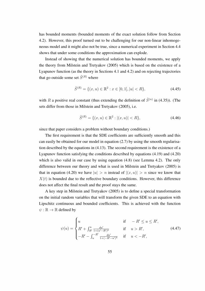
has bounded moments (bounded moments of the exact solution follow from Section4.2). However, this proof turned out to be challenging for our non-linear inhomoge-neous model and it might also not be true, since a numerical experiment in Section 4.4shows that under some conditions the approximation can explode.

Instead of showing that the numerical solution has bounded moments, we applythe theory from Milstein and Tretyakov (2005) which is based on the existence of aLyapunov function (as the theory in Sections 4.1 and 4.2) and on rejecting trajectoriesthat go outside some set S(R) where

S(R) = (x, u) ∈ R2 : x ∈ [0, 1], |u| < R, (4.45)

with R a positive real constant (thus extending the definition of S(n) in (4.35)). (Thesets differ from those in Milstein and Tretyakov (2005), i.e.

S(R) = (x, u) ∈ R2 : |(x, u)| < R, (4.46)

since that paper considers a problem without boundary conditions.)The first requirement is that the SDE coefficients are sufficiently smooth and this

can easily be obtained for our model in equation (2.7) by using the smooth regularisa-tion described by the equations in (4.13). The second requirement is the existence of aLyapunov function satisfying the conditions described by equations (4.19) and (4.20)which is also valid in our case by using equation (4.8) (see Lemma 4.2). The onlydifference between our theory and what is used in Milstein and Tretyakov (2005) isthat in equation (4.20) we have |u| > n instead of |(x, u)| > n since we know thatX(t) is bounded due to the reflective boundary conditions. However, this differencedoes not affect the final result and the proof stays the same.

A key step in Milstein and Tretyakov (2005) is to define a special transformationon the initial random variables that will transform the given SDE to an equation withLipschitz continuous and bounded coefficients. This is achieved with the functionψ : R→ R defined by

ψ(u) =

u if −R′ ≤ u ≤ R′,

R′ +∫ uR′

du′

1+(u′−R′)k if u > R′,

−R′ −∫ −R′u

du′

1+(−R′−u′)k if u < −R′,

(4.47)

55

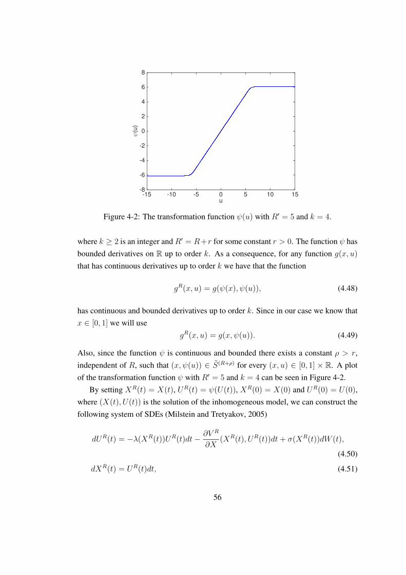
u-15 -10 -5 0 5 10 15

ψ(u

)

-8

-6

-4

-2

0

2

4

6

8

Figure 4-2: The transformation function ψ(u) with R′ = 5 and k = 4.

where k ≥ 2 is an integer andR′ = R+r for some constant r > 0. The function ψ hasbounded derivatives on R up to order k. As a consequence, for any function g(x, u)

that has continuous derivatives up to order k we have that the function

gR(x, u) = g(ψ(x), ψ(u)), (4.48)

has continuous and bounded derivatives up to order k. Since in our case we know thatx ∈ [0, 1] we will use

gR(x, u) = g(x, ψ(u)). (4.49)

Also, since the function ψ is continuous and bounded there exists a constant ρ > r,independent of R, such that (x, ψ(u)) ∈ S(R+ρ) for every (x, u) ∈ [0, 1] × R. A plotof the transformation function ψ with R′ = 5 and k = 4 can be seen in Figure 4-2.

By setting XR(t) = X(t), UR(t) = ψ(U(t)), XR(0) = X(0) and UR(0) = U(0),where (X(t), U(t)) is the solution of the inhomogeneous model, we can construct thefollowing system of SDEs (Milstein and Tretyakov, 2005)

dUR(t) = −λ(XR(t))UR(t)dt− ∂V R

∂X(XR(t), UR(t))dt+ σ(XR(t))dW (t),

(4.50)

dXR(t) = UR(t)dt, (4.51)

56

whose coefficients have bounded derivatives up to order k. The next proposition isthen proved in Milstein and Tretyakov (2005).

Proposition 4.12. Assume that F (x, u) satisfies (4.19), (4.20) and

minx∈[0,1],|u|≥R+ρ

F (x, u)

minx∈[0,1],|u|≥R

F (x, u)≤ α, (4.52)

where α is a constant independent of R. Let φ(x, u) be a function such that

limR→∞

maxx∈[0,1],|u|≤R

|φ(x, u)|

minx∈[0,1],|u|≥R

F (x, u)= 0. (4.53)

Then for all (X(0), U(0)) ∈ [0, 1]×R and all ε > 0 there exists R(X(0), U(0), ε) > 0

such that ∀R > R(X(0), U(0), ε)

∣∣E [φR(XR(T ), UR(T ))]− E [φ(X(T ), U(T ))]

∣∣ < ε. (4.54)

The significance of Proposition 4.12 is that we can construct a new regularisedmodel with Lipschitz continuous coefficients by introducing an arbitrarily small extraerror. With some simple algebra (see Lemma 4.13) we can easily see that this proposi-tion applies to our inhomogeneous problem since equation (4.8) and the quantities ofinterest defined in Section 2.4 satisfy the required conditions. The result from Propo-sition 4.12 will also be used later in Chapter 5 in the application of Theorem 3.1.

Lemma 4.13. The function

F (x, u) = 1 +1

2

u2

σ2U(x)

− 1

2log

σ2U(x)

(κσu∗)2, (4.55)

and the quantities of interest defined in Section 2.4 satisfy the conditions of Proposition

4.12 with R ≥ 1.

Proof . We have already seen in Lemma 4.2 and Theorem 4.5 that F (x, u) satisfies

57

(4.19) and (4.20). For inequality (4.52), we have

minx∈[0,1],|u|≥R+ρ

F (x, u)

minx∈[0,1],|u|≥R

F (x, u)=

minx∈[0,1],|u|≥R+ρ

1 + 1

2u2

σ2U (x)− 1

2log

σ2U (x)

(κσu∗)2

min

x∈[0,1],|u|≥R

1 + 1

2u2

σ2U (x)− 1

2log

σ2U (x)

(κσu∗)2

=

1 + (R+ρ)2

α1+ α2

1 + R2

α1+ α2

,

where α1 = maxx∈[0,1]

σ2U(x) and α2 = min

x∈[0,1]

−1

2log

σ2U (x)

(κσu∗)2

. Then,

minx∈[0,1],|u|≥R+ρ

F (x, u)

minx∈[0,1],|u|≥R

F (x, u)≤

1 + 2(R2+ρ2)α1

+ α2

1 + R2

α1+ α2

≤1 + 2(R2+ρ2)

α1+ α2

R2

α1

=α1

R2+ 2

(1 +

ρ2

R2

)+α1α2

R2

≤ α1 + 2(1 + ρ2

)+ α1α2 (since R ≥ 1).

The right hand side is independent of R so by setting it equal to α we obtain inequality(4.52).From Section 2.4 we have that φ(x, u) equals X(T ) or 1[a,b](X(T )) and therefore

maxx∈[0,1],|u|≤R

|φ(x, u)| = 1. (4.56)

Substituting in equation (4.53) gives

limR→∞

maxx∈[0,1],|u|≤R

|φ(x, u)|

minx∈[0,1],|u|≥R

F (x, u)= lim

R→∞

1

minx∈[0,1],|u|≥R

F (x, u)= 0, (4.57)

by property (4.20).

Finally, the following two assumptions on the timestepping method (in our caseSymplectic Euler, Geometric Langevin and BAOAB) used to discretise the Lipschitzcontinuous system of equations (4.50) and (4.51) are necessary before stating the mainconvergence theorem.

Assumption 4.14. The timestepping method applied to the regularised SDEs (4.50)

58

and (4.51) has a weak error (see Definition 4.11) of at least order 1 and after one

timestep the local weak error (i.e. Definition 4.11 after one timestep) is of at least

order 2.

Assumption 4.15. If (XRn , U

Rn ) ∈ S(R) for n = 0, . . . , k, where (XR

n , URn ) is the

approximation of the regularised SDEs (4.50) and (4.51) at time tn, then (Xn, Un) =

(XRn , U

Rn ) for n = 0, . . . , k.

And now we state the main convergence theorem from Milstein and Tretyakov(2005).

Theorem 4.16. Consider any timestepping method satisfying Assumption 4.14 which

converges with a weak error of order p for systems with sufficiently smooth and bounded

derivatives up to some order (e.g. order 4 for Euler-Maruyama). Let the conditions of

Proposition 4.12 and the Assumption 4.15 be fulfilled and consider a function φ(x, u)

such that E [|φ(X(T ), U(T ))|] exists. Then for all (X(0), U(0)) ∈ [0, 1]×R and ε > 0

there exists R(X(0), U(0), ε) > 0 such that ∀R ≥ R(X(0), U(0), ε) and sufficiently

small h

|E [φ(X(T ), U(T ))]− E [φ(XM , UM)1ΩR(ω)]| < Khp + ε, (4.58)

where ΩR = ω : (XRn , U

Rn ) ∈ S(R), n = 0, . . . ,M − 1 and (XR

M , URM) ∈ [0, 1] ×

[−R,R] and K > 0 depends on (X(0), U(0)) and R.

The only change we did in Theorem 4.16 is to assume that E [|φ(X(T ), U(T ))|]exists (true for our quantities of interest since the mean particle position and the con-centration are bounded) instead of assuming that |φ(x, u)| ≤ V (x, u). In Milstein andTretyakov (2005) the second assumption is used to prove the first assumption but if weassume directly that E [|φ(X(T ), U(T ))|] exists then Theorem 4.16 holds for a widerclass of functions φ(x, u).

The conclusion from Theorem 4.16 is that by rejecting the trajectories of particlesthat have a velocity with absolute value greater than R we can guarantee the weakconvergence of the timestepping method by just adding a small error. For example,when we use the Euler-Maruyama method, we have that equation (4.58) holds withp = 1. Note that increasing R decreases the extra error ε but at the same time it canalso increase K so h needs to be sufficiently small.

We already know that for the regularised SDEs (4.50) and (4.51), Assumption 4.14holds for the Euler-Maruyama method (Kloeden and Platen, 2011). In Section 4.3.2

59

we show that if Assumption 4.14 is true for the Euler-Maruyama method then it is alsotrue for all the timestepping methods defined in Section 3.1. Also, Assumption 4.15trivially holds for our timestepping methods since the coefficients of the original SDEsand the Lipschitz continuous system in equations (4.50) and (4.51) are equal on the setS(R).

4.3.2 A Taylor series expansion approach for weak convergence

With a Taylor series expansion approach we show that if the Euler-Maruyama methodconverges with a weak error of order 1 then the Symplectic Euler, Geometric Langevinand BAOAB methods also converge with at least the same order of weak error. Herewe only present the analysis for the Symplectic Euler method but a similar approachworks for Geometric Langevin and BAOAB (see Appendix A.3 for the GeometricLangevin method). Consequently, the convergence result from Milstein and Tretyakov(2005) (see Theorem 4.16) will also hold for the timestepping methods described inSection 3.1 when applied to the inhomogeneous model.

For our analysis we use the following theorem from Kloeden and Platen (2011) forthe weak convergence of a general timestepping method.

Theorem 4.17. Using the notation introduced at the beginning of Section 4.3, a method

converges with weak error of order α if the local error over one timestep satisfies

|E [φ(X(h))]− E [φ(X1)]| ≤ Chα+1, (4.59)

for all polynomials φ up to degree 2α + 1 and a constant C > 0.

For example, for the Euler-Maruyama method, Theorem 4.17 is true with α = 1

(see beginning of Section 4.3). Using Taylor series expansions we show that this isalso true for the Symplectic Euler, Geometric Langevin and BAOAB methods.

Firstly, let (XSE1 , USE

1 ) be the Symplectic Euler approximation to the exact solu-tion (X(h), U(h)) of the inhomogeneous model after one timestep as described byequations (3.1) and (3.2). Denote by (XEM

1 , UEM1 ) the corresponding approximation

for the Euler - Maruyama method. Our result for the Symplectic Euler method is thensummarised in the following theorem.

Corollary 4.18. If the Euler-Maruyama method applied to SDEs (2.7) and (2.8) con-

verges with a weak error of order 1 then the weak error of the Symplectic Euler method,

60

applied to the same equations, also converges with at least order 1.

Proof . Let φ be a polynomial as in Theorem 4.17. For the Symplectic Euler methodwe have

∣∣E [φ(X(h), U(h))]− E[φ(XSE

1 , USE1 )]∣∣ = |E [φ(X(h), U(h))]

− E[φ(X0 + USE

1 h, USE1 )]∣∣ , (4.60)

and since the only difference that Euler-Maruyama has, is that it usesXEM1 = X0+U0h

instead of XSE1 = X0 +USE

1 h we apply a Taylor series expansion on the first argumentof φ(X0 + USE

1 h, USE1 ). This gives

φ(X0 + USE1 h, USE

1 ) = φ(X0 + [(1− λ(X0)h)U0 −∂V

∂X(X0, U0)h+ σ(X0)

√hξ0]h, USE

1 )

= φ(X0 + U0h− λ(X0)U0h2 − ∂V

∂X(X0, U0)h2 + σ(X0)h

32 ξ0, U

SE1 )

= φ(X0 + U0h, USE1 )

+∂φ

∂X(X0 + U0h, U

SE1 )(−λ(X0)U0h

2 − ∂V

∂X(X0, U0)h2 + σ(X0)h

32 ξ0)

+ higher order terms.

Since we are interested in expectations we can neglect all higher order terms sincethey either have a mean zero or they are of order higher than h2. Substituting in (4.60)and using the fact that USE

1 = UEM1 , we obtain

∣∣E [φ(X(h), U(h))]− E[φ(XSE

1 , USE1 )]∣∣ = |E [φ(X(h), U(h))]

− E[φ(X0 + U0h, U

SE1 )]

+O(h2)∣∣

≤ |E [φ(X(h), U(h))]

− E[φ(X0 + U0h, U

SE1 )]∣∣+O(h2)

= |E [φ(X(h), U(h))]

− E[φ(XEM

1 , UEM1 )]∣∣+O(h2).

If the Euler-Maruyama method converges weakly with order 1 we have

∣∣E [φ(X(h), U(h))]− E[φ(XEM

1 , UEM1 )]∣∣ ≤ CEMh2, (4.61)

61

for some constant CEM > 0 which implies

∣∣E [φ(X(h), U(h))]− E[φ(XSE

1 , USE1 )]∣∣ = O(h2), (4.62)

and completes the proof by using Theorem 4.17.

The same approach as in Corollary 4.18 but with harder algebra also works forGeometric Langevin and BAOAB. See Appendix A.3 for the Geometric Langevinmethod.

Our conclusion is that for a system of SDEs with Lipschitz continuous, sufficientlysmooth and polynomially bounded coefficients we have that our timestepping methodsconverge with a weak error of order 1 (since the Euler-Maruyama does (Kloeden andPlaten, 2011)). As a result, by rejecting any exploding trajectories as described inMilstein and Tretyakov (2005) we can guarantee the convergence of our timesteppingmethods when applied to the inhomogeneous model. First order weak convergencewill also be used in Section 5.3.2 in the derivation of the modified equations (Shardlow,2006), (Zygalakis, 2011).

4.4 A simple numerical experiment with theSymplectic Euler method

Next, we present some simple numerical experiments to demonstrate that for our in-homogeneous model and values of U(0) which are physically valid, it is very unlikelythat the approximation of U(t) becomes large. Also, to show that it is possible to haveexplosive behaviour in extreme cases, we present an experiment with an unphysicallylarge value of U(0). Although the explosive behaviour that we observe might not berelated to the discussion of Section 4.3.1 and it is simply related to instability, i.e. thetimestep size is not small enough for the given U(0), we still present this experimentto show that it is unlikely to have any problems with our set of parameters.

We always use the Symplectic Euler method and the inhomogeneous model param-eters κσ = 1.3, κτ = 0.5, u∗ = 0.2, H = 1, εreg = 0.01km, T = 1 and X(0) = 0.05.The value of U(0) depends on the experiment. Denote by U (i)

n the approximation ofthe ith trajectory at time tn = nh.

For our first experiment we compute the maximum and minimum values of Un

62

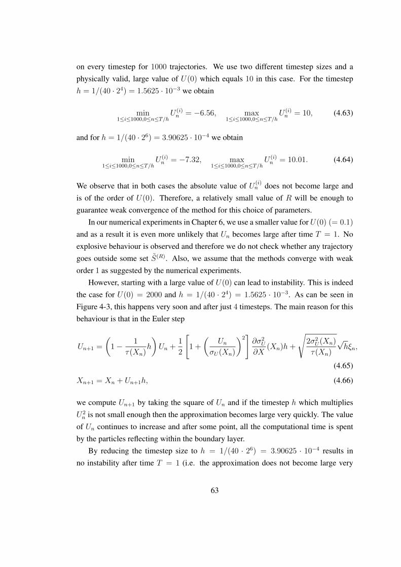
on every timestep for 1000 trajectories. We use two different timestep sizes and aphysically valid, large value of U(0) which equals 10 in this case. For the timesteph = 1/(40 · 24) = 1.5625 · 10−3 we obtain

min1≤i≤1000,0≤n≤T/h

U (i)n = −6.56, max

1≤i≤1000,0≤n≤T/hU (i)n = 10, (4.63)

and for h = 1/(40 · 26) = 3.90625 · 10−4 we obtain

min1≤i≤1000,0≤n≤T/h

U (i)n = −7.32, max

1≤i≤1000,0≤n≤T/hU (i)n = 10.01. (4.64)

We observe that in both cases the absolute value of U (i)n does not become large and

is of the order of U(0). Therefore, a relatively small value of R will be enough toguarantee weak convergence of the method for this choice of parameters.

In our numerical experiments in Chapter 6, we use a smaller value for U(0) (= 0.1)

and as a result it is even more unlikely that Un becomes large after time T = 1. Noexplosive behaviour is observed and therefore we do not check whether any trajectorygoes outside some set S(R). Also, we assume that the methods converge with weakorder 1 as suggested by the numerical experiments.

However, starting with a large value of U(0) can lead to instability. This is indeedthe case for U(0) = 2000 and h = 1/(40 · 24) = 1.5625 · 10−3. As can be seen inFigure 4-3, this happens very soon and after just 4 timesteps. The main reason for thisbehaviour is that in the Euler step

Un+1 =

(1− 1

τ(Xn)h

)Un +

1

2

[1 +

(Un

σU(Xn)

)2]∂σ2

U

∂X(Xn)h+

√2σ2

U(Xn)

τ(Xn)

√hξn,

(4.65)

Xn+1 = Xn + Un+1h, (4.66)

we compute Un+1 by taking the square of Un and if the timestep h which multipliesU2n is not small enough then the approximation becomes large very quickly. The value

of Un continues to increase and after some point, all the computational time is spentby the particles reflecting within the boundary layer.

By reducing the timestep size to h = 1/(40 · 26) = 3.90625 · 10−4 results inno instability after time T = 1 (i.e. the approximation does not become large very

63

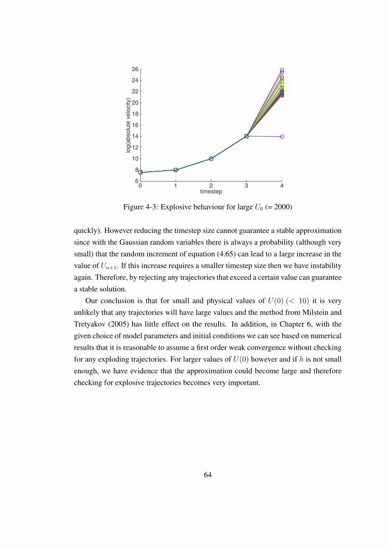
timestep0 1 2 3 4

log(a

bsolu

te v

elo

city)

6

8

10

12

14

16

18

20

22

24

26

Figure 4-3: Explosive behaviour for large U0 (= 2000)

quickly). However reducing the timestep size cannot guarantee a stable approximationsince with the Gaussian random variables there is always a probability (although verysmall) that the random increment of equation (4.65) can lead to a large increase in thevalue of Un+1. If this increase requires a smaller timestep size then we have instabilityagain. Therefore, by rejecting any trajectories that exceed a certain value can guaranteea stable solution.

Our conclusion is that for small and physical values of U(0) (< 10) it is veryunlikely that any trajectories will have large values and the method from Milstein andTretyakov (2005) has little effect on the results. In addition, in Chapter 6, with thegiven choice of model parameters and initial conditions we can see based on numericalresults that it is reasonable to assume a first order weak convergence without checkingfor any exploding trajectories. For larger values of U(0) however and if h is not smallenough, we have evidence that the approximation could become large and thereforechecking for explosive trajectories becomes very important.

64

Chapter 5

MLMC and the application of theComplexity Theorem

Our next topic is to study the theoretical application of Theorem 3.1 (complexity theo-rem, Giles (2008)) to the one-dimensional models that will enable us to determine theconditions under which the MLMC method gives a better asymptotic cost rate whencompared to StMC.

We begin from the homogeneous model and present a direct approach for thisapplication to a problem without reflection. We continue by presenting the theoret-ical analysis of a new treatment of reflective boundary conditions that preserves thequadratic MLMC variance decay which is one of the most important and hardest toshow requirements of Theorem 3.1. With this new algorithm that verifies numericallyTheorem 3.1, we then describe how a modified equations approach (Shardlow, 2006),(Zygalakis, 2011) (Muller et al., 2015) can be used to show the theoretical applicationto the inhomogeneous model.

Finally, we discuss how we deal with the discontinuity of the indicator functionin the concentration problem. This discontinuity causes an increase in the variancewhich reduces the performance of the MLMC. Therefore, it becomes necessary tofind a suitable approximation and our approach is to use smoothing poynomials (Gileset al., 2015), (Giles et al., 2017).

Some of these results have already been published in Katsiolides et al. (2018). Tothe best of our knowledge this is the first time that the theoretical application of Theo-rem 3.1 (complexity theorem, Giles (2008)) is studied for a problem from atmospheric

65

dispersion modelling.

5.1 Homogeneous model

Firstly, we prove that the conditions of Theorem 3.1 hold for the simplified modeland the Geometric Langevin method without boundary conditions using a uniformtimestep. For the problem with reflection, the application will follow with the specialboundary conditions treatment described later in Section 5.2. Also, without boundaryconditions the homogeneous model is a simple Ornstein-Uhlenbeck process for whicha well-defined exact solution exists. We do not include any results for the other twotimestepping methods since the simplified model is not the main focus of this thesis.

As a quantity of interest we take the mean particle position so in the notation usedin Section 3.2 we have that P = X(T ). We use the index (f) to denote the finestep approximations and the index (c) to denote the coarse step approximations. Fromthe simplified model equations (2.13), (2.14) and the discretisation method equations(3.8), (3.9) and (3.10) we have that on level l and n even the fine step becomes

U(f)n+1 = e−λhlU (f)

n + σαhlξn, (5.1)

X(f)n+1 = X(f)

n + U(f)n+1hl, (5.2)

and the coarse step

U(c)n+2 = e−2λhlU (c)

n + σα2hlξ?n, (5.3)

X(c)n+2 = X(c)

n + U(c)n+22hl, (5.4)

with αh =√

1−e−2λh

2λ, ξn ∼ Normal(0, 1) i.i.d. and ξ?n = rξn+ξn+1√

r2+1. Also let r = e−λhl .

The fine and coarse steps have the same initial conditions so

X(f)0 = X

(c)0 , U

(f)0 = U

(c)0 . (5.5)

Lemma 5.1. If the product λhl is small enough then conditions (i)− (iv) of Theorem

3.1 hold for the simplified model and the Geometric Langevin method.

Proof . The Geometric Langevin method, applied to the simplified model, is a firstorder method (Bou-Rabee and Owhadi, 2010) which implies that condition (i) fol-

66

lows. Clearly, condition (ii) follows from the definition of the MLMC method andthe linearity of expectation. Also, we know that the cost on each level is proportionalto the number of samples multiplied with the number of timesteps (since the cost pertimestep is fixed) and therefore condition (iv) follows. It only remains to prove thatcondition (iii) holds, i.e.

V ar[Yl,Nl ] ≤ CN−1l h2

l ,

for some positive constant C.From equation (5.2),

X(f)n+2 = X(f)

n +(U

(f)n+1 + U

(f)n+2

)hl, (5.6)

which implies using equation (5.4)

X(f)n+2 −X

(c)n+2 = X(f)

n −X(c)n +

(U

(f)n+1 + U

(f)n+2 − 2U

(c)n+2

)hl. (5.7)

From equation (5.1),

U(f)n+2 = r

(rU (f)

n + σ

√1− r2

2λξn

)+ σ

√1− r2

2λξn+1 (5.8)

= r2U (f)n + σr

√1− r2

2λξn + σ

√1− r2

2λξn+1, (5.9)

which implies using equation (5.3)

U(f)n+2 − U

(c)n+2 = r2U (f)

n + σ

√1− r2

2λ(rξn + ξn+1)− r2U (c)

n − σ√

1− r4

2λ

rξn + ξn+1√r2 + 1

= r2U (f)n + σ

√1− r2

2λ(rξn + ξn+1)− r2U (c)

n − σ√

1− r2

2λ(rξn + ξn+1)

= r2(U (f)n − U (c)

n

)= rn+2

(U

(f)0 − U (c)

0

)(by induction)

= 0.

67

Therefore, equation (5.7) now becomes

X(f)n+2 −X

(c)n+2 = X(f)

n −X(c)n +

(U

(f)n+1 − U

(c)n+2

)hl

= X(f)0 −X(c)

0 + hl

n2∑

m=0

(U

(f)n−2m+1 − U

(c)n−2m+2

)(by induction)

= hl

n2∑

m=0

(U

(f)n−2m+1 − U

(c)n−2m+2

)(sinceX(f)

0 = X(c)0 ). (5.10)

In order to evaluate the above sum we firstly compute the difference U (f)n+1 − U

(c)n+2.

From equation (5.1)

U(f)n+1 = r2U

(f)n−1 + σαhl (rξn−1 + ξn)

= rn+1U(f)0 + σαhl

n∑k=0

rn−kξk

= rn+1U(f)0 + σαhl

n2−1∑

k=0

(rn−2kξ2k + rn−2k−1ξ2k+1

)+ σαhlξn.

From equation (5.3)

U(c)n+2 = r4U

(c)n−2 + σα2hl

(r2ξ?n−2 + ξ?n

)= rn+2U

(c)0 + σα2hl

n2∑

k=0

r2(n2−k)ξ?2k

= rn+2U(c)0 + σα2hl

n2∑

k=0

r2(n2−k) rξ2k + ξ2k+1√

r2 + 1

= rn+2U(c)0 + σ

√1− r2

2λ

n2∑

k=0

rn−2k (rξ2k + ξ2k+1)

= rn+2U(c)0 + σαhl

n2∑

k=0

(rn−2k+1ξ2k + rn−2kξ2k+1

).

Subtracting the last two equations for U (f)n+1 and U (c)

n+2 we get

U(f)n+1 − U

(c)n+2 = rn+1U

(f)0 − rn+2U

(c)0

68

+ σαhl

n2−1∑

k=0

[(rn−2k − rn−2k+1

)ξ2k +

(rn−2k−1 − rn−2k

)ξ2k+1

]+ σαhlξn − σαhlrξn − σαhlξn+1

= rn+1U(f)0 − rn+2U

(c)0

+ σαhl

n2−1∑

k=0

[rn−2k(1− r)ξ2k + rn−2k−1(1− r)ξ2k+1

]+ σαhl(1− r)ξn − σαhlξn+1

= rn+1U(f)0 − rn+2U

(c)0

+ σαhl

(1− r)n2−1∑

k=0

(rn−2kξ2k + rn−2k−1ξ2k+1

)+ (1− r)ξn − ξn+1

.Substituting in equation (5.10) now gives

X(f)n+2 −X

(c)n+2 = hl

n2∑

m=0

[rn−2m+1U

(f)0 − rn−2m+2U

(c)0

+ σαhl[(1− r)

n2−m−1∑k=0

(rn−2m−2kξ2k + rn−2m−2k−1ξ2k+1)

+ (1− r)ξn−2m − ξn−2m+1

] ],

and taking the variance

V ar(X

(f)n+2 −X

(c)n+2

)= h2

l σ2α2

hlV ar

n2∑

m=0

[(1− r)

n2−m−1∑k=0

(rn−2m−2kξ2k + rn−2m−2k−1ξ2k+1)

+ (1− r)ξn−2m − ξn−2m+1

] = h2

l σ2α2

hl

[V ar

n2∑

m=0

[(1− r)

n2−m−1∑k=0

rn−2m−2kξ2k + (1− r)ξn−2m

]+ V ar

n2∑

m=0

[(1− r)

n2−m−1∑k=0

rn−2m−2k−1ξ2k+1 − ξn−2m+1

]](by independence of even and odd indexed random variables)

69

= h2l σ

2α2hl

[V ar

n2∑

m=0

[(1− r)

n2−m∑k=0

rn−2m−2kξ2k

]︸ ︷︷ ︸

A

+ V ar

n2∑

m=0

[(1− r)

n2−m−1∑k=0

rn−2m−2k−1ξ2k+1 − ξn−2m+1

]︸ ︷︷ ︸

B

].

Let us firstly consider sum A which contains all the even indexed random variables.By the construction of the sum and for a fixed integer l we can write the coefficientof ξ2l as (1 − r)f2l(r) where f2l(r) is a polynomial of r of degree at most n and withcoefficients 1, 0 or −1. Similarly, for the sum B we can write the coefficient of ξ2l+1

as (1− r)f2l+1(r)− 1. Therefore, V ar(X

(f)n+2 −X

(c)n+2

)can be written as

V ar(X

(f)n+2 −X

(c)n+2

)= h2

l σ2α2

hl

[V ar

(1− r)n2∑l=0

f2l(r)ξ2l

+ V ar

n2∑l=0

[(1− r)f2l+1(r)− 1

]ξ2l+1

]

= h2l σ

2α2hl

[(1− r)2

n2∑l=0

(f2l(r))2 +

n2∑l=0

[(1− r)f2l+1(r)− 1

]2]

(by independence)

≤ h2l σ

2α2hl

[(1− r)2

n2∑l=0

(f2l(r))2 +

n2∑l=0

[2(1− r)2(f2l+1(r))2 + 2

]].

By the triangle inequality we have that |fl(r)| ≤∑n

k=0 rk = 1−rn+1

1−r which implies that

V ar(X

(f)n+2 −X

(c)n+2

)≤ h2

l σ2α2

hl

[(1− r)2

n2∑l=0

(1− rn+1

1− r

)2

+

n2∑l=0

[2(1− r)2

(1− rn+1

1− r

)2

+ 2]]

= h2l σ

2α2hl

(n2

+ 1) [

(1− rn+1)2 + 2(1− rn+1)2 + 2].

(5.11)

70

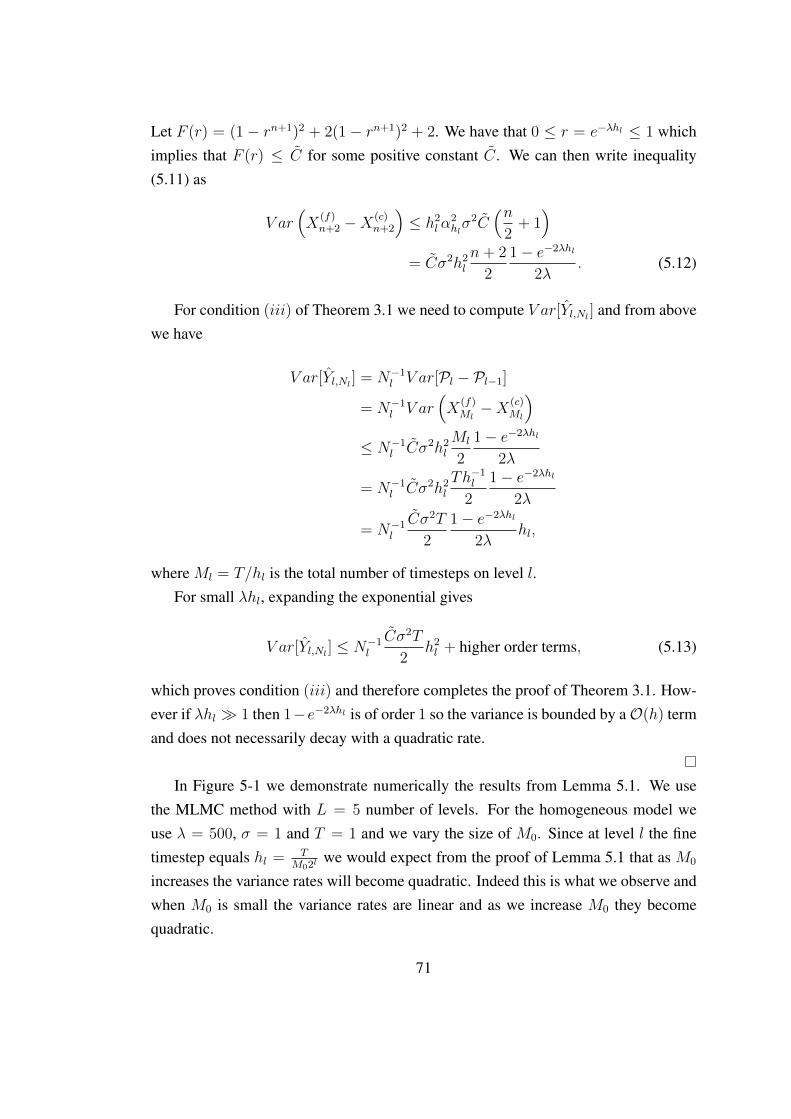
Let F (r) = (1− rn+1)2 + 2(1− rn+1)2 + 2. We have that 0 ≤ r = e−λhl ≤ 1 whichimplies that F (r) ≤ C for some positive constant C. We can then write inequality(5.11) as

V ar(X

(f)n+2 −X

(c)n+2

)≤ h2

lα2hlσ2C

(n2

+ 1)

= Cσ2h2l

n+ 2

2

1− e−2λhl

2λ. (5.12)

For condition (iii) of Theorem 3.1 we need to compute V ar[Yl,Nl ] and from abovewe have

V ar[Yl,Nl ] = N−1l V ar[Pl − Pl−1]

= N−1l V ar

(X

(f)Ml−X(c)

Ml

)≤ N−1

l Cσ2h2l

Ml

2

1− e−2λhl

2λ

= N−1l Cσ2h2

l

Th−1l

2

1− e−2λhl

2λ

= N−1l

Cσ2T

2

1− e−2λhl

2λhl,

where Ml = T/hl is the total number of timesteps on level l.For small λhl, expanding the exponential gives

V ar[Yl,Nl ] ≤ N−1l

Cσ2T

2h2l + higher order terms, (5.13)

which proves condition (iii) and therefore completes the proof of Theorem 3.1. How-ever if λhl 1 then 1−e−2λhl is of order 1 so the variance is bounded by aO(h) termand does not necessarily decay with a quadratic rate.

In Figure 5-1 we demonstrate numerically the results from Lemma 5.1. We usethe MLMC method with L = 5 number of levels. For the homogeneous model weuse λ = 500, σ = 1 and T = 1 and we vary the size of M0. Since at level l the finetimestep equals hl = T

M02lwe would expect from the proof of Lemma 5.1 that as M0

increases the variance rates will become quadratic. Indeed this is what we observe andwhen M0 is small the variance rates are linear and as we increase M0 they becomequadratic.

71

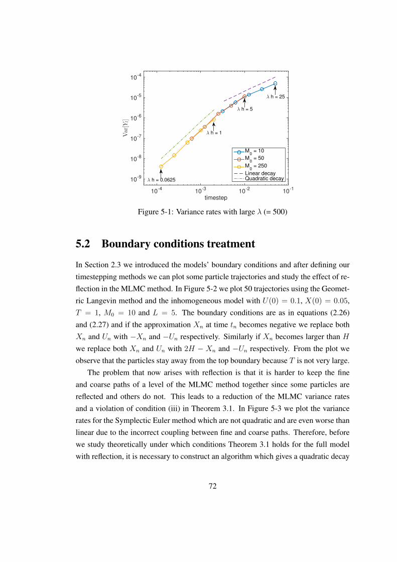
timestep10

-410

-310

-210

-1

Var[Y

l]

10-9

10-8

10-7

10-6

10-5

10-4

M0 = 10

M0 = 50

M0 = 250

Linear decayQuadratic decay

λ h = 25

λ h = 5

λ h = 1

λ h = 0.0625

Figure 5-1: Variance rates with large λ (= 500)

5.2 Boundary conditions treatment

In Section 2.3 we introduced the models’ boundary conditions and after defining ourtimestepping methods we can plot some particle trajectories and study the effect of re-flection in the MLMC method. In Figure 5-2 we plot 50 trajectories using the Geomet-ric Langevin method and the inhomogeneous model with U(0) = 0.1, X(0) = 0.05,T = 1, M0 = 10 and L = 5. The boundary conditions are as in equations (2.26)and (2.27) and if the approximation Xn at time tn becomes negative we replace bothXn and Un with −Xn and −Un respectively. Similarly if Xn becomes larger than Hwe replace both Xn and Un with 2H − Xn and −Un respectively. From the plot weobserve that the particles stay away from the top boundary because T is not very large.

The problem that now arises with reflection is that it is harder to keep the fineand coarse paths of a level of the MLMC method together since some particles arereflected and others do not. This leads to a reduction of the MLMC variance ratesand a violation of condition (iii) in Theorem 3.1. In Figure 5-3 we plot the variancerates for the Symplectic Euler method which are not quadratic and are even worse thanlinear due to the incorrect coupling between fine and coarse paths. Therefore, beforewe study theoretically under which conditions Theorem 3.1 holds for the full modelwith reflection, it is necessary to construct an algorithm which gives a quadratic decay

72

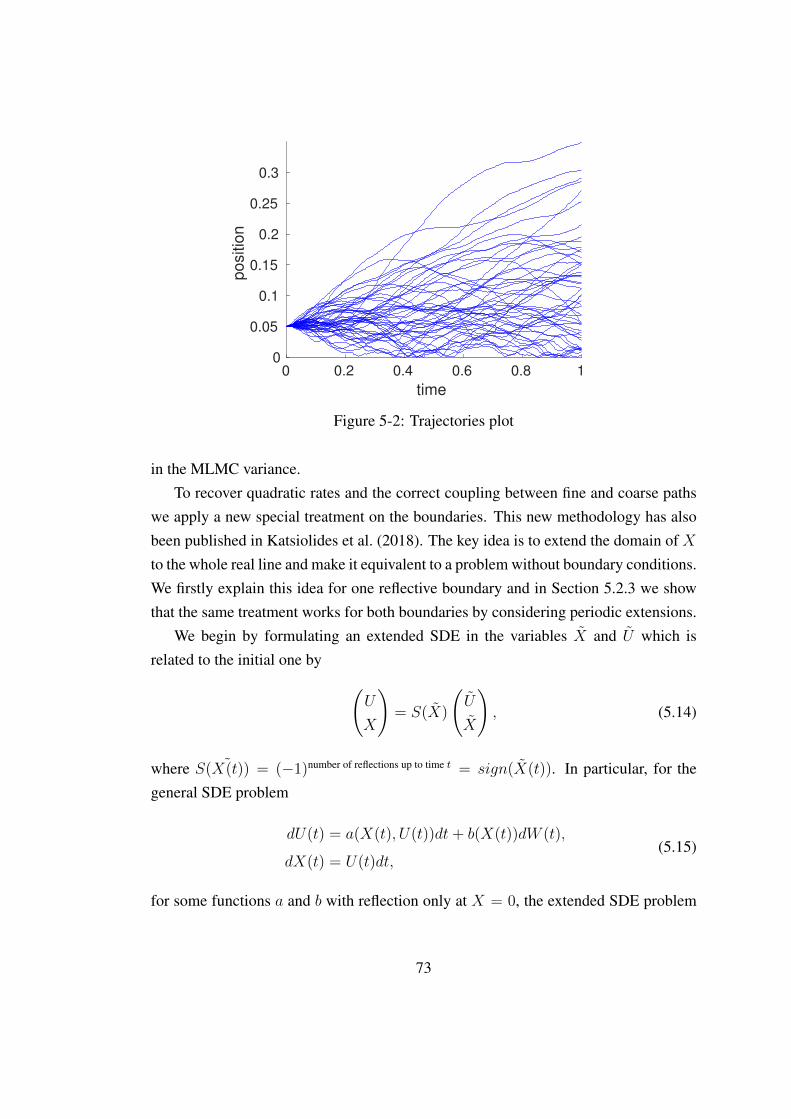
0 0.2 0.4 0.6 0.8 1

time

0

0.05

0.1

0.15

0.2

0.25

0.3

po

sitio

n

Figure 5-2: Trajectories plot

in the MLMC variance.To recover quadratic rates and the correct coupling between fine and coarse paths

we apply a new special treatment on the boundaries. This new methodology has alsobeen published in Katsiolides et al. (2018). The key idea is to extend the domain of Xto the whole real line and make it equivalent to a problem without boundary conditions.We firstly explain this idea for one reflective boundary and in Section 5.2.3 we showthat the same treatment works for both boundaries by considering periodic extensions.

We begin by formulating an extended SDE in the variables X and U which isrelated to the initial one by (

U

X

)= S(X)

(U

X

), (5.14)

where S( ˜X(t)) = (−1)number of reflections up to time t = sign(X(t)). In particular, for thegeneral SDE problem

dU(t) = a(X(t), U(t))dt+ b(X(t))dW (t),

dX(t) = U(t)dt,(5.15)

for some functions a and b with reflection only at X = 0, the extended SDE problem

73

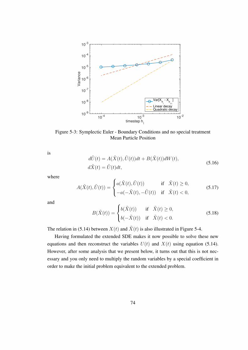
timestep hl

10-4

10-3

10-2

Va

rian

ce

10-9

10-8

10-7

10-6

10-5

10-4

10-3

Var[Xh

l

- Xh

l-1

]

Linear decayQuadratic decay

Figure 5-3: Symplectic Euler - Boundary Conditions and no special treatmentMean Particle Position

isdU(t) = A(X(t), U(t))dt+B(X(t))dW (t),

dX(t) = U(t)dt,(5.16)

where

A(X(t), U(t)) =

a(X(t), U(t)) if X(t) ≥ 0,

−a(−X(t),−U(t)) if X(t) < 0,(5.17)

and

B(X(t)) =

b(X(t)) if X(t) ≥ 0,

b(−X(t)) if X(t) < 0.(5.18)

The relation in (5.14) between X(t) and X(t) is also illustrated in Figure 5-4.Having formulated the extended SDE makes it now possible to solve these new

equations and then reconstruct the variables U(t) and X(t) using equation (5.14).However, after some analysis that we present below, it turns out that this is not nec-essary and you only need to multiply the random variables by a special coefficient inorder to make the initial problem equivalent to the extended problem.

74

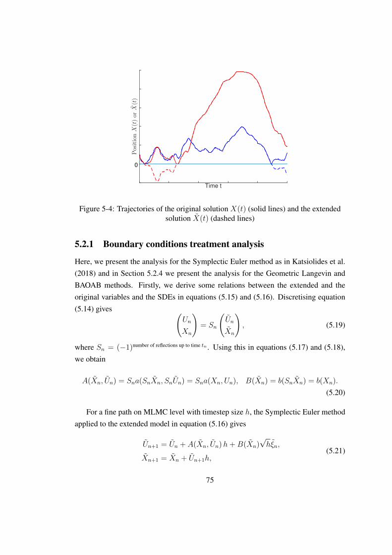
Time t

PositionX(t)or

X(t)

0

Figure 5-4: Trajectories of the original solution X(t) (solid lines) and the extendedsolution X(t) (dashed lines)

5.2.1 Boundary conditions treatment analysis

Here, we present the analysis for the Symplectic Euler method as in Katsiolides et al.(2018) and in Section 5.2.4 we present the analysis for the Geometric Langevin andBAOAB methods. Firstly, we derive some relations between the extended and theoriginal variables and the SDEs in equations (5.15) and (5.16). Discretising equation(5.14) gives (

Un

Xn

)= Sn

(Un

Xn

), (5.19)

where Sn = (−1)number of reflections up to time tn . Using this in equations (5.17) and (5.18),we obtain

A(Xn, Un) = Sna(SnXn, SnUn) = Sna(Xn, Un), B(Xn) = b(SnXn) = b(Xn).

(5.20)

For a fine path on MLMC level with timestep size h, the Symplectic Euler methodapplied to the extended model in equation (5.16) gives

Un+1 = Un + A(Xn, Un)h+B(Xn)√hξn,

Xn+1 = Xn + Un+1h,(5.21)

75

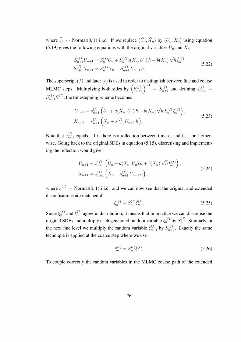
where ξn ∼ Normal(0, 1) i.i.d. If we replace (Un, Xn) by (Un, Xn) using equation(5.19) gives the following equations with the original variables Un and Xn

S(f)n+1Un+1 = S(f)

n Un + S(f)n a(Xn, Un)h+ b(Xn)

√h ξ(f)

n ,

S(f)n+1Xn+1 = S(f)

n Xn + S(f)n+1 Un+1 h,

(5.22)

The superscript (f) and later (c) is used in order to distinguish between fine and coarse

MLMC steps. Multiplying both sides by(S

(f)n+1

)−1

= S(f)n+1 and defining s

(f)n+1 =

S(f)n+1S

(f)n , the timestepping scheme becomes

Un+1 = s(f)n+1

(Un + a(Xn, Un)h+ b(Xn)

√hS(f)

n ξ(f)n

),

Xn+1 = s(f)n+1

(Xn + s

(f)n+1 Un+1 h

).

(5.23)

Note that s(f)n+1 equals −1 if there is a reflection between time tn and tn+1 or 1 other-

wise. Going back to the original SDEs in equation (5.15), discretising and implement-ing the reflection would give

Un+1 = s(f)n+1

(Un + a(Xn, Un)h+ b(Xn)

√h ξ(f)

n

),

Xn+1 = s(f)n+1

(Xn + s

(f)n+1 Un+1 h

),

(5.24)

where ξ(f)n ∼ Normal(0, 1) i.i.d. and we can now see that the original and extended

discretisations are matched ifξ(f)n = S(f)

n ξ(f)n . (5.25)

Since ξ(f)n and ξ(f)

n agree in distribution, it means that in practice we can discretise theoriginal SDEs and multiply each generated random variable ξ(f)

n by S(f)n . Similarly, in

the next fine level we multiply the random variable ξ(f)n+1 by S(f)

n+1. Exactly the sametechnique is applied at the coarse step where we use

ξ(c)n = S(c)

n ξ(c)n . (5.26)

To couple correctly the random variables in the MLMC coarse path of the extended

76

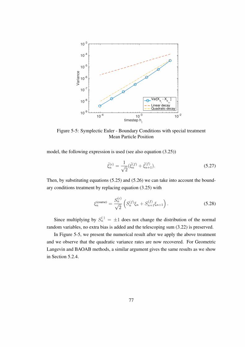
timestep hl

10-4

10-3

10-2

Va

rian

ce

10-9

10-8

10-7

10-6

10-5

10-4

10-3

Var[Xh

l

- Xh

l-1

]

Linear decayQuadratic decay

Figure 5-5: Symplectic Euler - Boundary Conditions with special treatmentMean Particle Position

model, the following expression is used (see also equation (3.25))

ξ(c)n =

1√2

(ξ(f)n + ξ

(f)n+1). (5.27)

Then, by substituting equations (5.25) and (5.26) we can take into account the bound-ary conditions treatment by replacing equation (3.25) with

ξ(coarse)n =

S(c)n√2

(S(f)n ξn + S

(f)n+1ξn+1

). (5.28)

Since multiplying by S(·)n = ±1 does not change the distribution of the normal

random variables, no extra bias is added and the telescoping sum (3.22) is preserved.In Figure 5-5, we present the numerical result after we apply the above treatment

and we observe that the quadratic variance rates are now recovered. For GeometricLangevin and BAOAB methods, a similar argument gives the same results as we showin Section 5.2.4.

77

5.2.2 Some comments on the discontinuities

Note that this treatment adds a discontinuity in the extended model since the functionA(X,U) is not continuous in general at X = 0 (since a(0, U) is not always equal to−a(0,−U) in equation (5.17)). For the inhomogeneous model and the Met Office’sconstant regularisation (equations (2.24) and (2.25)) no discontinuities are introducedby this treatment since the ∂V

∂X(X,U) term disappears when X = 0 and the λ(X)U

term stays continuous (in this case a(X,U) = −λ(X)U − ∂V∂X

(X,U)). However, wehave a discontinuity at X = εreg as shown in Figure 4-1a which is not a result of theboundary conditions treatment.

The opposite happens with the smooth regularisation described by the equations in(4.13) which is continuous at X = εreg. The only discontinuity is at X = 0 which is aresult of the boundary conditions treatment. In Section 5.3.2 we describe an alternativetype of smooth regularisation which gives continuous coefficients for both the originaland the extended inhomogeneous models.

In Chapter 6 all our numerical results are done by using the Met Office’s constantregularisation (equations (2.24) and (2.25)) and we didn’t observe any problems dueto the discontinuities. A theoretical study of the effect of these discontinuities can bea topic for future research. Finally, in Figure 5-6 we plot the extended inhomogeneousmodel coefficients with the Met Office’s constant regularisation.

5.2.3 Reflection at the top boundary

For the top boundary reflection we consider periodic extensions of the domain. ForX ∈ R, let

θ(X) = 2n if X ∈ [(2n− 1)H, (2n+ 1)H), n ∈ Z,

η(X) = X − θ(X)H.

Then, similarly to equations (5.17) and (5.18) we define the extended coefficients as

A(X(t), U(t)) =

a(η(X(t)), U(t)) if η(X(t)) ≥ 0,

−a(−η(X(t)),−U(t)) if η(X(t)) < 0,(5.29)

78

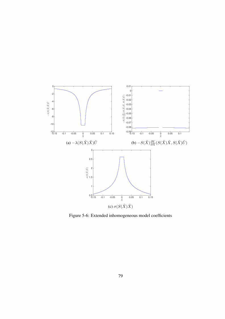
X

-0.15 -0.1 -0.05 0 0.05 0.1 0.15

−λ(S

(X)X

)U

-12

-10

-8

-6

-4

-2

0

(a) −λ(S(X)X)U

X

-0.15 -0.1 -0.05 0 0.05 0.1

−S(X

)∂V

∂X(S

(X)X

,S(X

)U)

-0.09

-0.08

-0.07

-0.06

-0.05

-0.04

-0.03

-0.02

-0.01

0

0.01

(b) −S(X) ∂V∂X (S(X)X, S(X)U)

X

-0.15 -0.1 -0.05 0 0.05 0.1 0.15

σ(S

(X)X

)

0.5

1

1.5

2

2.5

3

(c) σ(S(X)X)

Figure 5-6: Extended inhomogeneous model coefficients

79

and

B(X(t)) =

b(η(X(t))) if η(X(t)) ≥ 0,

b(−η(X(t))) if η(X(t)) < 0.(5.30)

It is now easy to see that η(X) reduces the problem to the case of reflecting only atX = 0 since this function brings X to the interval [−H,H]. Therefore, the sameanalysis applies and no further changes are required in equations (5.28) and (5.41)where S(·)

n now counts reflections at both boundaries.

5.2.4 Boundary conditions treatment for Geometric Langevinand BAOAB

Since Geometric Langevin and BAOAB are specialised methods for the Langevinequation we firstly consider an extended inhomogeneous turbulence model. This modelwill have the form of a Langevin equation. Again, we consider reflection only at thelower boundary and the top boundary treatment follows from periodic extensions as inSection 5.2.3. The results for the splitting methods form an extension of the analysispresented in Section 5.2.1.

The extended inhomogeneous turbulence model

Following the previous notation we can write the extended SDE coefficients in equa-tions (5.17) and (5.18) as

A(X(t), U(t)) = S(X(t))a(S(X(t))X(t), S(X(t))U(t)), (5.31)

B(X(t)) = b(S(X(t))X(t)). (5.32)

For the inhomogeneous turbulence model we have

a(X,U) = −λ(X)U − ∂V

∂X(X,U), b(X) = σ(X), (5.33)

80

so the extended inhomogeneous turbulence model is

dU(t) =− λ(S(X(t))X(t))U(t)dt− S(X(t))∂V

∂X

(S(X(t))X(t), S(X(t))U(t)

)dt

+ σ(S(X(t))X(t)

)dW (t), (5.34)

dX(t) = U(t)dt. (5.35)

Geometric Langevin

Firstly we consider the reflection treatment for the Geometric Langevin timesteppingmethod. Since the extended inhomogeneous turbulence model equations (5.34) and(5.35) have the form of a Langevin equation, we can apply directly the GeometricLangevin discretisation scheme given by equations (3.8), (3.9) and (3.10). This gives

U?n+1 = e−λ(SnXn)hUn + σ(SnXn)ah(SnXn)ξn,

Un+1 = U?n+1 − Sn

∂V

∂X

(SnXn, SnU

?n+1

)h,

Xn+1 = Xn + Un+1h,

where ah(SnXn) =√

1−e−2λ(SnXn)h

2λ(SnXn)and ξn ∼ Normal(0, 1). This scheme can also be

written as

Un+1 = e−λ(SnXn)hUn − Sn∂V

∂X

(SnXn, Sn

[e−λ(SnXn)hUn + σ(SnXn)ah(SnXn)ξn

])h

+ σ(SnXn)ah(SnXn)ξn,

Xn+1 = Xn + Un+1h.

Using equation (5.19),

Sn+1Un+1 = e−λ(Xn)hSnUn − Sn∂V

∂X

(Xn, Sn

[e−λ(Xn)hSnUn + σ(Xn)ah(Xn)ξn

])h

+ σ(Xn)ah(Xn)ξn,

Sn+1Xn+1 = SnXn + Sn+1Un+1h.

Letting sn+1 = Sn+1Sn we obtain the Geometric Langevin discretisation scheme for

81

the extended model

Un+1 = sn+1

[e−λ(Xn)hUn −

∂V

∂X

(Xn, e

−λ(Xn)hUn + σ(Xn)ah(Xn)Snξn

)h

+ σ(Xn)ah(Xn)Snξn

], (5.36)

Xn+1 = sn+1 (Xn + sn+1Un+1h) . (5.37)

Note that sn+1 equals −1 if there is a reflection between time tn and tn+1 or 1 other-wise.

The Geometric Langevin discretisation scheme for the original model with reflec-tion is given by

Un+1 = sn+1

[e−λ(Xn)hUn −

∂V

∂X

(Xn, e

−λ(Xn)hUn + σ(Xn)ah(Xn)ξn)h+ σ(Xn)ah(Xn)ξn

],

(5.38)

Xn+1 = sn+1 (Xn + sn+1Un+1h) , (5.39)

where ξn ∼ Normal(0, 1).Comparing equations (5.36), (5.37) with equations (5.38), (5.39) we can see that

the original and extended discretisations are matched if

ξn = Snξn, (5.40)

which is the same as in the case of Symplectic Euler method. Then, by followingthe same analysis as in Section (5.2.1) and by considering the fine and coarse MLMCsteps (and the same arguments after equation (5.25)) we deduce that the same treat-ment works for the Geometric Langevin method. Therefore, we only need to replaceequation (3.26) with

ξ(coarse)n = S(c)

n

e−λ(Xn)hS(f)n ξn + S

(f)n+1ξn+1√

e−2λ(Xn)h + 1, (5.41)

where S(f)n and S(c)

n count reflections on the fine and coarse steps respectively.

82

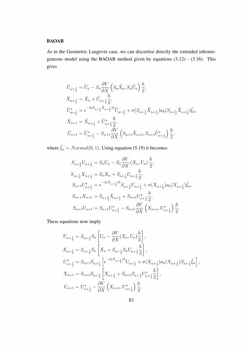
BAOAB

As in the Geometric Langevin case, we can discretise directly the extended inhomo-geneous model using the BAOAB method given by equations (3.12) - (3.16). Thisgives

Un+ 12

= Un − Sn∂V

∂X

(SnXn, SnUn

) h2,

Xn+ 12

= Xn + Un+ 12

h

2,

U?n+ 1

2= e

−λ(Sn+ 1

2Xn+ 1

2)hUn+ 1

2+ σ(Sn+ 1

2Xn+ 1

2)ah(Sn+ 1

2Xn+ 1

2)ξn,

Xn+1 = Xn+ 12

+ U?n+ 1

2

h

2,

Un+1 = U?n+ 1

2− Sn+1

∂V

∂X

(Sn+1Xn+1, Sn+1U

?n+ 1

2

) h2,

where ξn ∼ Normal(0, 1). Using equation (5.19) it becomes

Sn+ 12Un+ 1

2= SnUn − Sn

∂V

∂X(Xn, Un)

h

2,

Sn+ 12Xn+ 1

2= SnXn + Sn+ 1

2Un+ 1

2

h

2,

Sn+1U?n+ 1

2= e

−λ(Xn+ 1

2)hSn+ 1

2Un+ 1

2+ σ(Xn+ 1

2)ah(Xn+ 1

2)ξn,

Sn+1Xn+1 = Sn+ 12Xn+ 1

2+ Sn+1U

?n+ 1

2

h

2,

Sn+1Un+1 = Sn+1U?n+ 1

2− Sn+1

∂V

∂X

(Xn+1, U

?n+ 1

2

) h2.

These equations now imply

Un+ 12

= Sn+ 12Sn

[Un −

∂V

∂X(Xn, Un)

h

2

],

Xn+ 12

= Sn+ 12Sn

[Xn + Sn+ 1

2SnUn+ 1

2

h

2

],

U?n+ 1

2= Sn+1Sn+ 1

2

[e−λ(X

n+ 12

)hUn+ 1

2+ σ(Xn+ 1

2)ah(Xn+ 1

2)Sn+ 1

2ξn

],

Xn+1 = Sn+1Sn+ 12

[Xn+ 1

2+ Sn+1Sn+ 1

2U?n+ 1

2

h

2

],

Un+1 = U?n+ 1

2− ∂V

∂X

(Xn+1, U

?n+ 1

2

) h2.

83

The discretisation scheme for the original model with reflection is

Un+ 12

= Sn+ 12Sn

[Un −

∂V

∂X(Xn, Un)

h

2

],

Xn+ 12

= Sn+ 12Sn

(Xn + Sn+ 1

2SnUn+ 1

2

h

2

),

U?n+ 1

2= Sn+1Sn+ 1

2

[e−λ(X

n+ 12

)hUn+ 1

2+ σ(Xn+ 1

2)ah(Xn+ 1

2)ξn

],

Xn+1 = Sn+1Sn+ 12

(Xn+ 1

2+ Sn+1Sn+ 1

2U?n+ 1

2

h

2

),

Un+1 = U?n+ 1

2− ∂V

∂X

(Xn+1, U

?n+ 1

2

) h2,

where ξn ∼ Normal(0, 1).Comparing the discretisation schemes for the original and extended models we can

see that they are matched ifξn = Sn+ 1

2ξn. (5.42)

The variable Sn+ 12

counts the number of reflections just before the Ornstein-Uhlenbeckstep. Equation (5.42) was also derived in the Geometric Langevin case and implies thatthe same treatment works. Therefore, we use the random variable

ξ(coarse)n = S(c)

n

e−λ(Xn)hS(f)n ξn + S

(f)n+1ξn+1√

e−2λ(Xn)h + 1, (5.43)

for the MLMC coarse step.

5.2.5 Some final comments

As a final note in the boundary conditions treatment section, we briefly discuss a prob-lem that might appear when discretising SDEs with reflection, as described in Ramliand Esler (2016). The authors of Ramli and Esler (2016) studied a problem aris-ing with reflective boundary conditions when timestepping methods with intermediatesteps (like for example Geometric Langevin and BAOAB) are used to discretise theinhomogeneous model equations (2.7) and (2.8). In particular, when the timestep sizewas not small enough, some errors due to reflective boundary conditions arised thatdominated the discretisation and sampling errors of their higher order schemes thatinvolve intermediate timesteps.

84

Since this problem was about timestepping methods with intermediate steps, it ispossible that it might also affect our timestepping methods and in particular GeometricLangevin and BAOAB. In order to solve this issue, a simple method is described inRamli and Esler (2016). Firstly, at the start of each timestep, the domain of X isextended to (−∞,∞) by repeated reflection of σU(x) and τ(x). All intermediatesteps are then completed in the extended domain and at the end of the full timestepthe particle is taken back in [0, 1] using reflection as described in the first paragraphof Section 5.2. This treatment then removes any problems with reflective boundaryconditions.

In our numerical experiments we did not observe this issue when using any ofthe two timestepping methods and therefore it was not necessary to apply the methoddescribed in Ramli and Esler (2016). Further investigation however on this problemand how it affects MLMC performance can be a topic for future work.

5.3 Inhomogeneous model and the complexitytheorem

We now study the theoretical application of Theorem 3.1 (complexity theorem, Giles(2008)) to the inhomogeneous model with reflection and in particular to the extendedmodel as described in Section 5.2. A direct approach to apply Theorem 3.1 as we didfor the homogeneous model in Section 5.1 is very difficult and challenging due to thefact that the inhomogeneous model is a non-linear SDE. Here, we study an alternativeapproach based on the theory of modified equations (Shardlow, 2006), (Zygalakis,2011) and their application to the MLMC method. As described in Muller et al. (2015),modified equations provide an alternative method to check whether the conditions ofTheorem 3.1 hold which does not directly rely on strong approximation results.

5.3.1 Modified equations and the complexity theorem

We begin by defining the modified equations (Shardlow, 2006), (Zygalakis, 2011).Consider the general SDE

dX(t) = f(X(t))dt+G(X(t))dW(t), (5.44)

85

with X(t) ∈ Rd, f : Rd → Rd, G : Rd → Rd×m and initial conditions X(0). Supposethat for some timestepping method (eg Euler method) we can compute a first orderweak approximation XM(M = T/h) of X(T ), i.e.

|E [φ(X(T ))]− E [φ(XM)]| ≤ Ch, (5.45)

for some constant C > 0 and for all suitable test functions φ : Rd → R (this can begeneralised to pth order). Under some conditions (Shardlow, 2006), (Zygalakis, 2011)it is then possible to compute functions f1 : Rd → Rd and G1 : Rd → Rd×m andconstruct a modified SDE

dXh(t) =(f(Xh(t)) + hf1(Xh(t))

)dt+

(G(Xh(t)) + hG1(Xh(t))

)dW(t), (5.46)

such that the approximation XM is a second order weak approximation to the exactsolution Xh(t) of (5.46), i.e.

∣∣E [φ(Xh(T ))]− E [φ(XM)]

∣∣ ≤ Ch2, (5.47)

for some constant C > 0 and test functions φ. The functions f1 and G1 depend on thecoefficient functions in equation (5.44) and on the timestepping method.

The most important property of the modified equations is that with a small pertur-bation of the original SDE we can construct a new system of equations such that thetimestepping method approximates its solution more accurately. This property is oneof the key ideas considered in Muller et al. (2015) in order to provide an alternativeapproach for the application of Theorem 3.1.

In particular, in Muller et al. (2015) they consider the following doubled-up systemof SDEs

dX(t) = f(X(t))dt+G(X(t))dW(t), (5.48)

dY(t) = f(Y(t))dt+G(Y(t))dW(t), Y(0) = X(0). (5.49)

The two equations have the same initial conditions and Brownian motion W(t). Equa-tion (5.48) will be discretised with a timestep size h/2 as in the MLMC fine step andequation (5.49) will be discretised with a timestep size h as in the MLMC coarse step.The reason why we discretise with both the fine and coarse schemes is to add informa-

86

tion about the random variable coupling (eg equation (3.26) for Geometric Langevin)in the MLMC coarse step. As we already discussed in Section 3.2.2, the random vari-able coupling affects property (iii) of Theorem 3.1 (quadratic variance decay rate) andtherefore it is necessary to be taken into account in the proof. Then, following thetechnique from Zygalakis (2011) we compute modified equations of the form

dXh(t) =(f(Xh(t)) + hf1(Xh(t))

)dt+

(G(Xh(t)) + hG1(Xh(t))

)dW(t),

(5.50)

dYh(t) =(f(Yh(t)) + hf2(Yh(t))

)dt+

(G(Yh(t)) + hG2(Yh(t))

)dW(t),

(5.51)

with initial conditions Xh(0) = X(0),Yh(0) = X(0). The functions fi : Rd → Rd

and Gi : Rd → Rd×m for i = 1, 2. Also, let Z(t) = [X(t),Y(t)] be the exact solutionof equations (5.48) and (5.49) and denote its approximation by Zn = [Xn,Yn]. Thefollowing lemma is then proved in Muller et al. (2015) (Lemma 3.3).

Lemma 5.2. For t ∈ [0, T ], let Z(t) satisfy the SDEs (5.48) and (5.49) and let Zh(t) =

[Xh(t),Yh(t)] satisfy the modified equations (5.50) and (5.51). Suppose that

(i) f : Rd → Rd and G : Rd → Rd×m are globally Lipschitz continuous with

Lipschitz constant L > 0.

(ii) There exists C1 > 0 such that, for all h > 0 suffciently small,

E[∥∥f1(Xh(s))

∥∥2],E[∥∥G1(Xh(s))

∥∥2

F

]≤ C1,

E[∥∥f2(Yh(s))

∥∥2],E[∥∥G2(Yh(s))

∥∥2

F

]≤ C1, s ∈ [0, T ],

where ‖·‖F denotes the Frobenius norm.

Then, if ψ : R2d → R is globally Lipschitz continuous, we have for some constant

C2 > 0 independent of h,

E[∣∣ψ(Z(t))− ψ(Zh(t))

∣∣2] ≤ C2h2, for t ∈ [0, T ]. (5.52)

As it is noted in Muller et al. (2015), a sufficient condition for the regularity as-sumptions of Lemma 5.2 to hold, is that the coefficients f , fi, G and Gi are globally

87

Lipschitz continuous.In the next theorem, we can see how the modified equations and the regularity

conditions of Lemma 5.2 can be used to show that Theorem 3.1 holds.

Theorem 5.3. Fix T > 0. Let φ : Rd → R be globally Lipschitz continuous and

infinitely differentiable with polynomially bounded derivatives. Suppose that

(i) Xn and Yn are weak order-α approximations to X(t) for some α > 1/2 (see

also Definition 4.11),

(ii) Zn are second-order weak approximations to Zh(t) and

(iii) the assumptions of Lemma 5.2 hold.

Then Conditions (i) − (iii) of Theorem 3.1 (MLMC complexity theorem) hold with

[P(i)l ,P(i)

l−1] given by i.i.d. samples of [φ(XMl), φ(YMl

)] with h = hl and (XMl,YMl

)

the approximation of (XT ,YT ).

Proof . See Theorem 3.4 in Muller et al. (2015).The conclusion of Theorem 5.3 is that with the existence of a second-order modi-

fied equation and with some regularity conditions on the SDE coefficients we can provethat the conditions of Theorem 3.1 hold. Therefore, as a result of Theorem 3.1, we ex-pect to see a O(ε−2) cost rate for MLMC that improves the corresponding cost rateof StMC which is O(ε−3) (see Section 3.2.1 for the StMC cost rate). In the next sec-tion, we apply this modified equations theory to the extended inhomogeneous modelequations (5.34) and (5.35) and study under which conditions Theorem 3.1 holds.

5.3.2 Application to the inhomogeneous model

We are now going to study the application of the modified equations theory to theextended inhomogeneous model described in Section 5.2. We only consider reflectionat the lower boundary but a similar approach also works for the top boundary. Forconvenience we begin by writing down the extended inhomogeneous model as derivedin Section 5.2.4. This is given by

dU(t) =− λ(S(X(t))X(t))U(t)dt− S(X(t))∂V

∂X

(S(X(t))X(t), S(X(t))U(t)

)dt

+ σ(S(X(t))X(t)

)dW (t), (5.53)

dX(t) = U(t)dt. (5.54)

88

where S(X(t)) = (−1)number of reflections up to time t = sign(X(t)).As Theorem 5.3 suggests, we firstly look for second order modified equations of

(5.53) and (5.54) with λ(X), ∂V∂X

(X,U) and σ(X) defined by (2.9) and (2.10). InZygalakis (2011) a general technique for deriving modified equations is described forSDEs with smooth coefficients. In particular, for a first order timestepping method it ispossible in some cases to derive a second order modified equation (can be generalisedto higher orders).

Looking at equations (5.53) and (5.54) we can easily see that the SDE coefficientsare not smooth and some of them are also discontinuous and the reason for this is thepresence of the function S(X(t)) = sign(X(t)). To solve this problem we can applya special regularisation of the functions σU(X) and τ(X) in the SDE coefficients

λ(X) =1

τ(X), σ(X) =

√2σ2

U(X)

τ(X), (5.55)

∂V (X,U)

∂X= −1

2

[1 +

(U

σU(X)

)2]∂σ2

U(X)

∂X. (5.56)

As described in Section 2.2, regularising the SDE coefficients means to replace themwith some similar functions in order to make sure that the timestepping methods re-main stable. In addition, it can make the model easier to analyse theoretically. Insteadof using a constant regularisation as the Met Office does (equations (2.24) and (2.25)),we replace σU(X) and τ(X) with some functions σεreg

U (X) and τ εreg(X) on the intervals[0, εreg] and [H − εreg, H]. These functions have the following properties

τ(εreg) = τ εreg(εreg),∂τ

∂X(εreg) =

∂τ εreg

∂X(εreg),

∂τ εreg

∂X(0) = 0, (5.57)

and

σU(εreg) = σεregU (εreg),

∂σU∂X

(εreg) =∂σ

εregU

∂X(εreg), (5.58)

∂σεregU

∂X(0) = 0,

∂2σU∂X2

(εreg) =∂2σ

εregU

∂X2(εreg), (5.59)

with similar changes for the upper interval. These conditions guarantee that the coeffi-cients of the extended model are continuously differentiable. If we need continuity forhigher order derivatives then we can just add similar conditions on higher order deriva-tives of σεreg

U (X) and τ εreg(X). For simplicity we can assume that σεregU (X) and τ εreg(X)

89

are polynomials of sufficiently high degree and use the above conditions to solve asimultaneous system of linear equations that will give the polynomial coefficients.

With this choice of regularisation we satisfy the first condition from Zygalakis(2011) that requires SDEs with smooth coefficients. The second condition is the exis-tence of a timestepping method which is weakly convergent with order 1. From Kloe-den and Platen (2011) we know that the Euler-Maruyama method and consequentlyall the other methods considered in this thesis as discussed in Section 4.3.2, convergeweakly with order 1 if the SDE coefficients are Lipschitz continuous, satisfy lineargrowth and have polynomially bounded derivatives up to order 4. So far we only havesmoothness of the coefficients, but all other requirements will follow if we also ap-ply the special transformation from Milstein and Tretyakov (2005) given by equation(4.47) which will give us coefficients with bounded derivarives. The combination ofour special regularisation (according to equations (5.57), (5.58) and (5.59)) with thetransformation from Milstein and Tretyakov (2005) results in SDE coefficients whichare continuously differentiable and bounded up to a sufficiently high degree. As aresult, the SDE coefficients will become Lipschitz continuous (this follows from theMean Value Theorem) which means that our timestepping methods converge weaklywith order 1. According to Proposition 4.12, approximating this new regularised SDEonly adds a small error.

For the rest of this chapter we assume that the coefficients of the extended modelequations (5.53) and (5.54) are Lipschitz continuous and have polynomially boundedderivatives up to order 4. To simplify the notation we rewrite the extended model as

dU(t) = −λ(X(t))U(t)dt− ∂V

∂X(X(t), U(t))dt+ σ(X(t))dW (t), (5.60)

dX(t) = U(t)dt, (5.61)

where λ, σ and ∂V∂X

take into account all the necessary regularisations and transforma-tions on the coefficients as discussed above. (X(t), U(t)) will be the solution of theextended model after we apply these changes on the coefficients. Finally, we can applythe analysis from Zygalakis (2011) to compute modified equations of the doubled-upsystem

dU(t) = −λ(X(t))U(t)dt− ∂V

∂X(X(t), U(t))dt+ σ(X(t))dW (t), (5.62)

90

dX(t) = U(t)dt, (5.63)

du(t) = −λ(x(t))u(t)dt− ∂V

∂x(x(t), u(t))dt+ σ(x(t))dW (t), (5.64)

dx(t) = u(t)dt. (5.65)

The modified equations have the form

dU(t) =

(−λ(X(t))U(t)− ∂V

∂X(X(t), U(t)) + hv

(U)1 (X(t), U(t))

)dt

+(σ(X(t)) + hΣ

(U)1 (X(t), U(t))

)dW (t), (5.66)

dX(t) =(U(t) + hv

(X)1 (X(t), U(t))

)dt+ hΣ

(X)1 (X(t), U(t))dW (t), (5.67)

du(t) =

(−λ(x(t))u(t)− ∂V

∂x(x(t), u(t)) + hv

(u)2 (x(t), u(t))

)dt

+(σ(x(t)) + hΣ

(u)2 (x(t), u(t))

)dW (t), (5.68)

dx(t) =(u(t) + hv

(x)2 (x(t), u(t))

)dt+ hΣ

(x)2 (x(t), u(t))dW (t). (5.69)

Due to the assumptions we have just made, the analysis applies for our threetimestepping methods and the modified equations can be computed using a com-puter algebra system. Here we give a brief description of the main steps and thereader is referred to Zygalakis (2011) for the full details. To compute the coeffi-cients of the modified equations we developed Python code that can be downloadedfrom https://bitbucket.org/em459/modified-equations. When the coef-ficients are computed they are extracted to a LATEX file which can also be found in theabove link. The names of some of the basic classes from this code are used in thetext below in order to explain how the modified equations are computed. Note that thecode can also compute modified equations for a single level timestepping method butin this thesis we focus only on doubled-up systems of equations. The user can computea single system or a doubled-up system of modified equations by either choosing theclass TimestepSinglelevel() or the class TimestepMultilevel().

Following the technique from Zygalakis (2011), the first step is to compute thegenerator L0 of the doubled-up system of equations (5.62)-(5.65) (this is done with thefunction L0(·) from the Python code). For our SDEs the generator L0 is given by thefollowing definition

91

Definition 5.4. The generator L0 of the doubled-up system of equations (5.62)-(5.65)is defined by

L0F = −(λ(X)U +

∂V

∂X(X,U)

)∂F

∂U+ U

∂F

∂X+σ2(X)

2

∂2F

∂U2

−(λ(x)u+

∂V

∂x(x, u)

)∂F

∂u+ u

∂F

∂x+σ2(x)

2

∂2F

∂u2

+ σ(X)σ(x)∂2F

∂U∂u,

(5.70)

where F (X,U, x, u) is a twice differentiable function.

The second step is to compute the operatorA1 (see Section 3.2 in Zygalakis (2011))that involves taking the expectation of the Taylor expansion with respect to h of thefunction φ(U

(f)2h , X

(f)2h , u

(c)2h , x

(c)2h ), for some test function φ. U (f)

2h , X(f)2h are the approx-

imations of U(2h), X(2h) after two fine steps of size h and u(c)2h , x

(c)2h are the approxi-

mations of u(2h), x(2h) after one coarse step of size 2h. Their form depends on thetimestepping method and this is the output of the classes TimestepSymplecticEuler(·),TimestepGeometricLangevinEuler(·) and TimestepBAOAB(·) as can be seen in thecode. The function A1(·) then takes these approximations and produces the Taylorexpansion.

The third step after computing the generator L0 and operator A1 is to computeA1φ − 1

2L2

0φ = A1φ − 12L0(L0φ) (see equation (3.9) in Zygalakis (2011)) and this is

done by the function L1(·) of our Python code.If we consider the generator Lh0 of the modified SDEs (5.66)-(5.69) (the equivalent

of L0 for (5.62)-(5.65)) we can write (Zygalakis, 2011)

Lh0 = L0 + hL1 + h2L2, (5.71)

for some generators L1,L2 and with L0 as in Definition 5.4. We then have that L1φ =

A1φ − 12L2

0φ and the comparison between L1φ and A1φ − 12L2

0φ gives the modifiedequations coefficients which are then extracted to a LATEX file.

For Symplectic Euler, the modified equations coefficients are given by

v(U)1 (X, U) =

U2

4

dλ

dX(X)− U

4λ2(X)− U

4λ(X)

∂2V

∂U∂X(X, U) +

U

4

∂2V

∂X2(X, U)

− 1

4

∂V

∂X(X, U)λ(X)− 1

4

∂V

∂X(X, U)

∂2V

∂U∂X(X, U)

92

+1

8σ2(X)

∂3V

∂U2∂X(X, U),

v(X)1 (X, U) = − U

4λ(X)− 1

4

∂V

∂X(X, U),

Σ(U)1 (X, U) = − U

4

dσ

dX(X) +

1

4λ(X)σ(X) +

1

4σ(X)

∂2V

∂U∂X(X, U),

Σ(X)1 (X, U) =

1

4σ(X),

v(u)2 (x, u) =

u2

2

dλ

dx(x)− u

2λ2(x)− u

2λ(x)

∂2V

∂u∂x(x, u) +

u

2

∂2V

∂x2(x, u)

− 1

2

∂V

∂x(x, u)λ(x)− 1

2

∂V

∂x(x, u)

∂2V

∂u∂x(x, u) +

1

4σ2(x)

∂3V

∂u2∂x(x, u),

v(x)2 (x, u) = − u

2λ(x)− 1

2

∂V

∂x(x, u),

Σ(u)2 (x, u) = − u

2

dσ

dx(x) +

1

2λ(x)σ(x) +

1

2σ(x)

∂2V

∂u∂x(x, u),

Σ(x)2 (x, u) =

1

2σ(x).

With the computation of the modified equations we now have that for the SymplecticEuler method the first two conditions from Theorem 5.3 hold. Also, with the assump-tions made on the coefficients of the original model we have that the newly computedcoefficients of the modified equations are Lipschitz continuous which means that thefinal condition from Theorem 5.3 holds. Therefore, we can apply Theorem 3.1 to theextended inhomogeneous model with the Symplectic Euler timestepping method andexpect to see a O(ε−2) cost rate for MLMC.

For the Geometric Langevin method we obtain similar modified equations coeffi-cients given by

v(U)1 (X, U) =

U2

4

dλ

dX¯(X) +

U

4λ(X)

∂2V

∂U∂X(X, U) +

U

4

∂2V

∂X2(X, U)

− 1

4

∂V

∂X(X, U)λ(X)− 1

4

∂V

∂X(X, U)

∂2V

∂U∂X(X, U)

− 1

8σ2(X)

∂3V

∂U2∂X(X, U),

v(X)1 (X, U) = − U

4λ(X)− 1

4

∂V

∂X(X, U),

Σ(U)1 (X, U) = − U

4

dσ

dX(X)− 1

4σ(X)

∂2V

∂U∂X(X, U),

93

Σ(X)1 (X, U) =

1

4σ(X),

v(u)2 (x, u) =

u2

2

dλ

dx(x) +

u

2λ(x)

∂2V

∂u∂x(x, u) +

u

2

∂2V

∂x2(x, u)− 1

2

∂V

∂x(x, u)λ(x)

− 1

2

∂V

∂x(x, u)

∂2V

∂u∂x(x, u)− 1

4σ2(x)

∂3V

∂u2∂x(x, u),

v(x)2 (x, u) = − u

2λ(x)− 1

2

∂V

∂x(x, u),

Σ(u)2 (x, u) = − u

2

dσ

dx(x)− 1

2σ(x)

∂2V

∂u∂x(x, u),

Σ(x)2 (x, u) =

1

2σ(x).

Finally, for BAOAB the modified equations coefficients have much fewer terms andthese are given by

v(U)1 (X, U) = −1

8

∂V

∂X(X, U)

∂2V

∂U∂X(X, U),

v(X)1 (X, U) = 0,

Σ(U)1 (X, U) = 0,

Σ(X)1 (X, U) = 0,

v(u)2 (x, u) = −1

4

∂V

∂x(x, u)

∂2V

∂u∂x(x, u),

v(x)2 (x, u) = 0,

Σ(u)2 (x, u) = 0,

Σ(x)2 (x, u) = 0.

As an aside, note that for the Euler-Maruyama method and when σ(X) is not constant,it is not possible to compute modified equations as shown in Zygalakis (2011).

Although we expect to see O(ε−2) cost rates for MLMC for all three timesteppingmethods, there is something important to note about BAOAB. For this method, almostall correction terms are zero and adding just one term in the original SDE gives themodified equations. This implies that we expect to see a smaller bias error for a fixedtimestep size when compared to Symplectic Euler and Geometric Langevin since theBAOAB method is just one term away from being a second order method while for-mally is still first order. This is an important property that we study further in Chapter6 where we observe in practice a much better performance. Most importantly, the

94

correction terms of BAOAB are independent of λ which diverges at the lower bound-ary. This is not true for the other two methods. This means that when λ is large thecorrection terms of Symplectic Euler and Geometric Langevin are not of order h andtherefore a smaller timestep is required (which increases the cost) in order to have asecond order weak error for the modified equations.

As we will see in Chapter 6, Theorem 3.1 still holds numerically without usingany special regularisation or transformation on the SDE coefficients. Therefore, forpractical applications is not necessary to apply any of them on the SDE coefficients.All the numerical results presented later are about the original model with the specialboundary conditions treatment (Section 5.2) and the Met Office’s constant regularisa-tion (equations (2.24) and (2.25)). All results from Section 5.3 can then be used toprovide a better understanding about the theoretical background of the problem.

5.4 Smoothing polynomials for the concentrationproblem

The last topic that we study in this chapter is the particle concentration. In Section2.4 we defined the indicator function which can be used as a quantity of interest toestimate the concentration of particles which land in an interval [a, b] after some timeT . Mathematically it can be written as

E[1[a,b](X(T ))

]. (5.72)

This is a very important quantity and one of the main interests in atmospheric disper-sion modelling as it measures the probability that a particle ends up in a certain region.Therefore, by knowing how many particles are released from the source enables us toestimate how many of them will end up in each region after time T . At the Met Officefor example, they might be interested in the ash particle concentration after a volcaniceruption which will determine whether it is safe or not for airplanes to travel.

The discontinuity of the indicator function at the boundaries of the interval [a, b]

causes an increase in the variance which reduces the efficiency of the MLMC method.In Figure 5-7 we plot the variance rates for the Geometric Langevin method which arelinear and therefore condition (iii) of Theorem 3.1 does not hold. As a result, we donot expect to see the improved cost rates of O(ε−2) when we run the MLMC method.

95

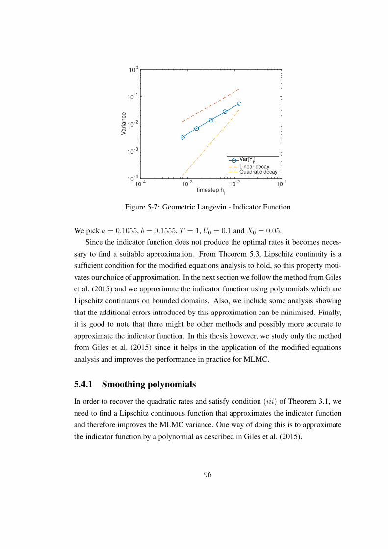
timestep hl

10-4

10-3

10-2

10-1

Va

rian

ce

10-4

10-3

10-2

10-1

100

Var[Yl]

Linear decayQuadratic decay

Figure 5-7: Geometric Langevin - Indicator Function

We pick a = 0.1055, b = 0.1555, T = 1, U0 = 0.1 and X0 = 0.05.Since the indicator function does not produce the optimal rates it becomes neces-

sary to find a suitable approximation. From Theorem 5.3, Lipschitz continuity is asufficient condition for the modified equations analysis to hold, so this property moti-vates our choice of approximation. In the next section we follow the method from Gileset al. (2015) and we approximate the indicator function using polynomials which areLipschitz continuous on bounded domains. Also, we include some analysis showingthat the additional errors introduced by this approximation can be minimised. Finally,it is good to note that there might be other methods and possibly more accurate toapproximate the indicator function. In this thesis however, we study only the methodfrom Giles et al. (2015) since it helps in the application of the modified equationsanalysis and improves the performance in practice for MLMC.

5.4.1 Smoothing polynomials

In order to recover the quadratic rates and satisfy condition (iii) of Theorem 3.1, weneed to find a Lipschitz continuous function that approximates the indicator functionand therefore improves the MLMC variance. One way of doing this is to approximatethe indicator function by a polynomial as described in Giles et al. (2015).

96

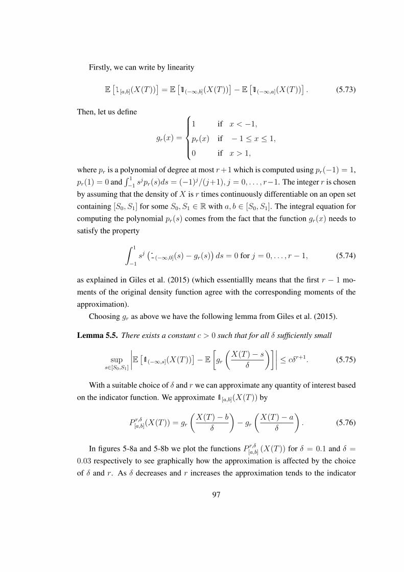
Firstly, we can write by linearity

E[1[a,b](X(T ))

]= E

[1(−∞,b](X(T ))

]− E

[1(−∞,a](X(T ))

]. (5.73)

Then, let us define

gr(x) =

1 if x < −1,

pr(x) if − 1 ≤ x ≤ 1,

0 if x > 1,

where pr is a polynomial of degree at most r+1 which is computed using pr(−1) = 1,pr(1) = 0 and

∫ 1

−1sjpr(s)ds = (−1)j/(j+1), j = 0, . . . , r−1. The integer r is chosen

by assuming that the density of X is r times continuously differentiable on an open setcontaining [S0, S1] for some S0, S1 ∈ R with a, b ∈ [S0, S1]. The integral equation forcomputing the polynomial pr(s) comes from the fact that the function gr(x) needs tosatisfy the property∫ 1

−1

sj(1(−∞,0](s)− gr(s)

)ds = 0 for j = 0, . . . , r − 1, (5.74)

as explained in Giles et al. (2015) (which essentiallly means that the first r − 1 mo-ments of the original density function agree with the corresponding moments of theapproximation).

Choosing gr as above we have the following lemma from Giles et al. (2015).

Lemma 5.5. There exists a constant c > 0 such that for all δ sufficiently small

sups∈[S0,S1]

∣∣∣∣E [1(−∞,s](X(T ))]− E

[gr

(X(T )− s

δ

)]∣∣∣∣ ≤ cδr+1. (5.75)

With a suitable choice of δ and r we can approximate any quantity of interest basedon the indicator function. We approximate 1[a,b](X(T )) by

P r,δ[a,b](X(T )) = gr

(X(T )− b

δ

)− gr

(X(T )− a

δ

). (5.76)

In figures 5-8a and 5-8b we plot the functions P r,δ[a,b] (X(T )) for δ = 0.1 and δ =

0.03 respectively to see graphically how the approximation is affected by the choiceof δ and r. As δ decreases and r increases the approximation tends to the indicator

97

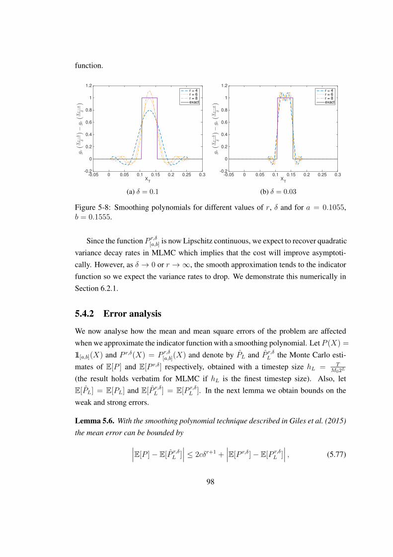
function.

XT

-0.05 0 0.05 0.1 0.15 0.2 0.25 0.3

gr

(

XT−b

δ

)

−gr

(

XT−a

δ

)

-0.2

0

0.2

0.4

0.6

0.8

1

1.2

r = 4

r = 6

r = 8

exact

(a) δ = 0.1

XT

-0.05 0 0.05 0.1 0.15 0.2 0.25 0.3

gr

(

XT−b

δ

)

−gr

(

XT−a

δ

)

-0.2

0

0.2

0.4

0.6

0.8

1

1.2

r = 4

r = 6

r = 8

exact

(b) δ = 0.03

Figure 5-8: Smoothing polynomials for different values of r, δ and for a = 0.1055,b = 0.1555.

Since the function P r,δ[a,b] is now Lipschitz continuous, we expect to recover quadratic

variance decay rates in MLMC which implies that the cost will improve asymptoti-cally. However, as δ → 0 or r →∞, the smooth approximation tends to the indicatorfunction so we expect the variance rates to drop. We demonstrate this numerically inSection 6.2.1.

5.4.2 Error analysis

We now analyse how the mean and mean square errors of the problem are affectedwhen we approximate the indicator function with a smoothing polynomial. Let P (X) =

1[a,b](X) and P r,δ(X) = P r,δ[a,b](X) and denote by PL and P r,δ

L the Monte Carlo esti-mates of E[P ] and E[P r,δ] respectively, obtained with a timestep size hL = T

M02L

(the result holds verbatim for MLMC if hL is the finest timestep size). Also, letE[PL] = E[PL] and E[P r,δ

L ] = E[P r,δL ]. In the next lemma we obtain bounds on the

weak and strong errors.

Lemma 5.6. With the smoothing polynomial technique described in Giles et al. (2015)

the mean error can be bounded by∣∣∣E[P ]− E[P r,δL ]∣∣∣ ≤ 2cδr+1 +

∣∣∣E[P r,δ]− E[P r,δL ]∣∣∣ , (5.77)

98

and the mean square error by

E[(P r,δL − E[P ]

)2]≤ V ar(P r,δ

L ) +(E[P r,δ

L ]− E[P r,δ])2

+ 4c2δ2(r+1)

+ 4cδr+1∣∣∣E[P r,δ

L ]− E[P r,δ]∣∣∣ , (5.78)

where δ and r are as defined in Section 5.4.1 and c is the constant in (5.75).

Proof . We firstly consider the following difference between the expected values ofthe indicator function P and the smoothed function P r,δ

∣∣E[P ]− E[P r,δ]∣∣ ≤ ∣∣∣∣E [1(−∞,b](XT )

]− E

[gr

(XT − bδ

)]∣∣∣∣+

∣∣∣∣E [1(−∞,a](XT )]− E

[gr

(XT − a

δ

)]∣∣∣∣≤ cδr+1 + cδr+1

= 2cδr+1. (5.79)

Using this expression and the unbiasedness of the Monte Carlo estimator P r,δL , the

mean error bound is∣∣∣E[P ]− E[P r,δL ]∣∣∣ ≤ ∣∣E[P ]− E[P r,δ]

∣∣+∣∣∣E[P r,δ]− E[P r,δ

L ]∣∣∣

≤ 2cδr+1 +∣∣∣E[P r,δ]− E[P r,δ

L ]∣∣∣ .

For the mean square error we write

P r,δL − E[P ] =

(P r,δL − E[P r,δ

L ])

+(E[P r,δ

L ]− E[P r,δ])

+(E[P r,δ]− E[P ]

),

and then we obtain using inequality (5.79)

E[(P r,δL − E[P ]

)2]

= Var(P r,δL ) +

(E[P r,δ

L ]− E[P r,δ])2

+(E[P r,δ]− E[P ]

)2

+ 2(E[P r,δ

L ]− E[P r,δ]) (

E[P r,δ]− E[P ]])

≤ Var(P r,δL ) +

(E[P r,δ

L ]− E[P r,δ])2

+ 4c2δ2(r+1)

99

+ 4cδr+1∣∣∣E[P r,δ

L ]− E[P r,δ]∣∣∣ . (5.80)

From the mean square error bound we observe that if δ is small enough and r

is large enough, the last two terms become small and the error is dominated by thefirst two terms which represent the sampling error and the discretisation error as inthe case of the indicator function without smoothing (see equations (3.18) and (3.27)).Therefore, we can reduce any additional smoothing errors by choosing suitable δ andr. At the same time however we need to be careful not to choose a very small δ ora very large r since the smoothing polynomial approximation will be closer to theindicator function which will cause an increase in the MLMC variance. The effect ofδ and r on the MLMC variance is studied numerically in Section 6.2.1.

100

Chapter 6

Numerical Results

After our theoretical study of the one-dimensional models in Chapters 4 and 5 we nowpresent some numerical results that will enable us to compare the efficiency of Stan-dard and Multilevel Monte Carlo with our three timestepping methods. We includeresults only for the one-dimensional inhomogeneous model (equations (2.7) and (2.8))with the Met Office’s regularisation as described in Section 2.2 and the special bound-ary conditions treatment as described in Section 5.2. To be more precise, we do notapply any special regularisation or transformation in the SDE coefficients from thosedescribed in Chapters 4 and 5 and these ideas are only used for the theoretical results.As we see, Theorem 3.1 and the convergence of the timestepping methods still holdnumerically without the theoretical assumptions on the SDE coefficients.

In Sections 6.1, 6.2 and 6.3 we study the mean particle position, concentrationin an interval [a, b] and a piecewise constant approximation of the concentration fieldrespectively at the final time T . We use the three timestepping methods described inSection 3.1 and a uniform timestep. In Section 6.4 we also investigate the effect ofadaptive timestepping.

The results are generated using the C++ code initially developed for the paperMuller et al. (2015) and which we later enriched for the purposes of this thesis. Thecode can be downloaded freely under the GPL license from https://bitbucket.

org/em459/mlmclangevin. The numerical results and conclusions of this chaptercan also be found in Katsiolides et al. (2018) and were obtained with the version whichhas been archived as Mueller et al. (2017). All plots in this chapter are obtained fromKatsiolides et al. (2018) and we follow the same structure as in sections 6 and 7 from

101

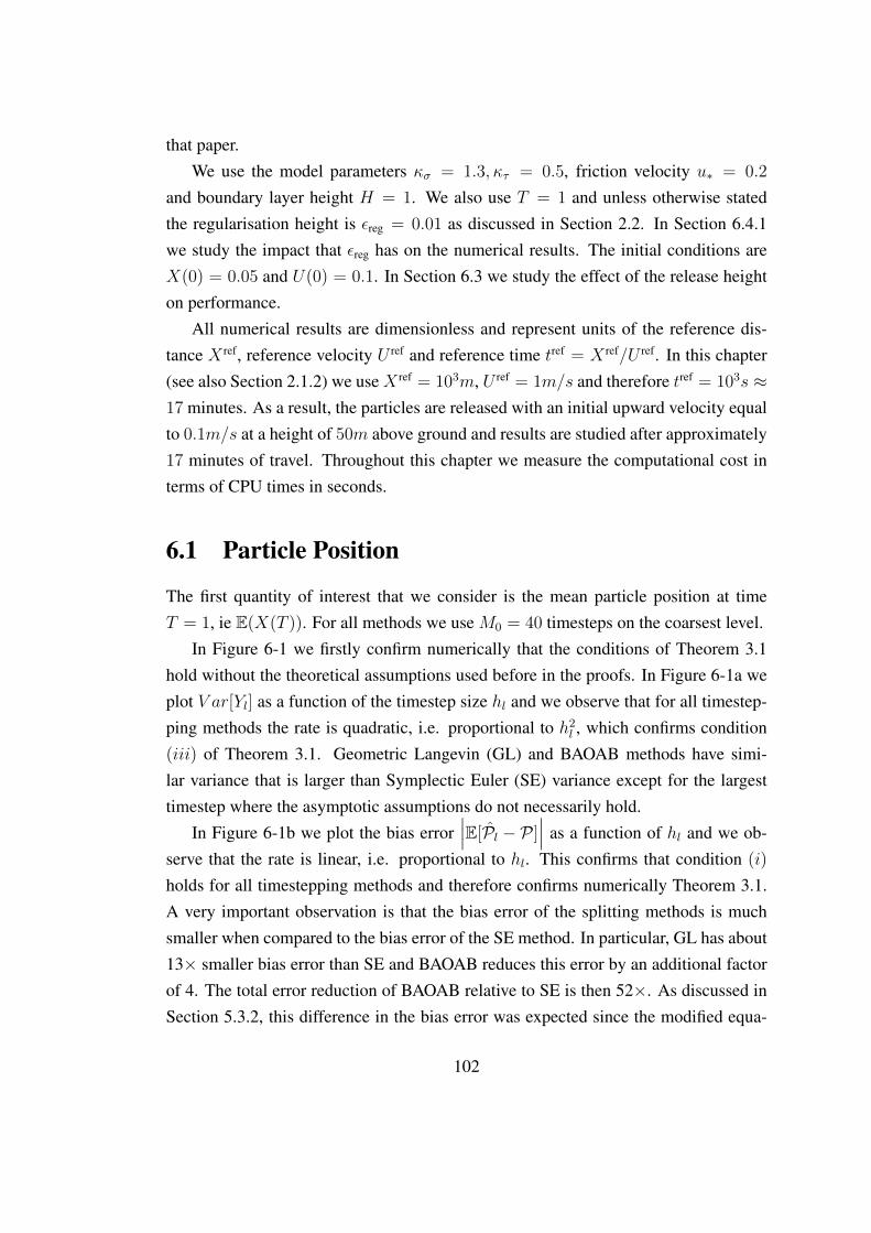
that paper.We use the model parameters κσ = 1.3, κτ = 0.5, friction velocity u∗ = 0.2

and boundary layer height H = 1. We also use T = 1 and unless otherwise statedthe regularisation height is εreg = 0.01 as discussed in Section 2.2. In Section 6.4.1we study the impact that εreg has on the numerical results. The initial conditions areX(0) = 0.05 and U(0) = 0.1. In Section 6.3 we study the effect of the release heighton performance.

All numerical results are dimensionless and represent units of the reference dis-tance X ref, reference velocity U ref and reference time tref = X ref/U ref. In this chapter(see also Section 2.1.2) we use X ref = 103m, U ref = 1m/s and therefore tref = 103s ≈17 minutes. As a result, the particles are released with an initial upward velocity equalto 0.1m/s at a height of 50m above ground and results are studied after approximately17 minutes of travel. Throughout this chapter we measure the computational cost interms of CPU times in seconds.

6.1 Particle Position

The first quantity of interest that we consider is the mean particle position at timeT = 1, ie E(X(T )). For all methods we use M0 = 40 timesteps on the coarsest level.

In Figure 6-1 we firstly confirm numerically that the conditions of Theorem 3.1hold without the theoretical assumptions used before in the proofs. In Figure 6-1a weplot V ar[Yl] as a function of the timestep size hl and we observe that for all timestep-ping methods the rate is quadratic, i.e. proportional to h2

l , which confirms condition(iii) of Theorem 3.1. Geometric Langevin (GL) and BAOAB methods have simi-lar variance that is larger than Symplectic Euler (SE) variance except for the largesttimestep where the asymptotic assumptions do not necessarily hold.

In Figure 6-1b we plot the bias error∣∣∣E[Pl − P ]

∣∣∣ as a function of hl and we ob-serve that the rate is linear, i.e. proportional to hl. This confirms that condition (i)

holds for all timestepping methods and therefore confirms numerically Theorem 3.1.A very important observation is that the bias error of the splitting methods is muchsmaller when compared to the bias error of the SE method. In particular, GL has about13× smaller bias error than SE and BAOAB reduces this error by an additional factorof 4. The total error reduction of BAOAB relative to SE is then 52×. As discussed inSection 5.3.2, this difference in the bias error was expected since the modified equa-

102

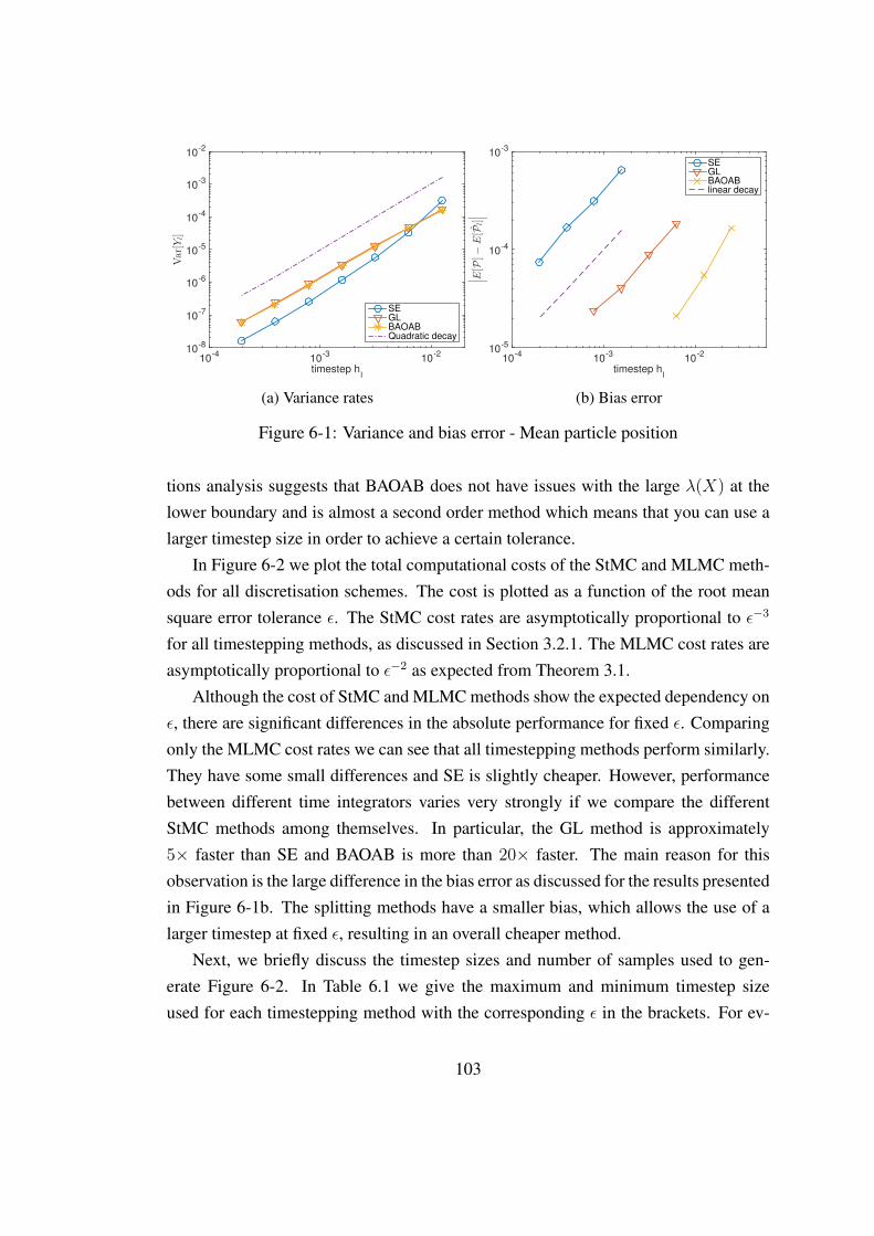
timestep hl

10-4

10-3

10-2

Var[Yl]

10-8

10-7

10-6

10-5

10-4

10-3

10-2

SEGLBAOABQuadratic decay

(a) Variance rates

timestep hl

10-4

10-3

10-2

∣ ∣ ∣E[P

]−E[P

l]∣ ∣ ∣

10-5

10-4

10-3

SEGLBAOABlinear decay

(b) Bias error

Figure 6-1: Variance and bias error - Mean particle position

tions analysis suggests that BAOAB does not have issues with the large λ(X) at thelower boundary and is almost a second order method which means that you can use alarger timestep size in order to achieve a certain tolerance.

In Figure 6-2 we plot the total computational costs of the StMC and MLMC meth-ods for all discretisation schemes. The cost is plotted as a function of the root meansquare error tolerance ε. The StMC cost rates are asymptotically proportional to ε−3

for all timestepping methods, as discussed in Section 3.2.1. The MLMC cost rates areasymptotically proportional to ε−2 as expected from Theorem 3.1.

Although the cost of StMC and MLMC methods show the expected dependency onε, there are significant differences in the absolute performance for fixed ε. Comparingonly the MLMC cost rates we can see that all timestepping methods perform similarly.They have some small differences and SE is slightly cheaper. However, performancebetween different time integrators varies very strongly if we compare the differentStMC methods among themselves. In particular, the GL method is approximately5× faster than SE and BAOAB is more than 20× faster. The main reason for thisobservation is the large difference in the bias error as discussed for the results presentedin Figure 6-1b. The splitting methods have a smaller bias, which allows the use of alarger timestep at fixed ε, resulting in an overall cheaper method.

Next, we briefly discuss the timestep sizes and number of samples used to gen-erate Figure 6-2. In Table 6.1 we give the maximum and minimum timestep sizeused for each timestepping method with the corresponding ε in the brackets. For ev-

103

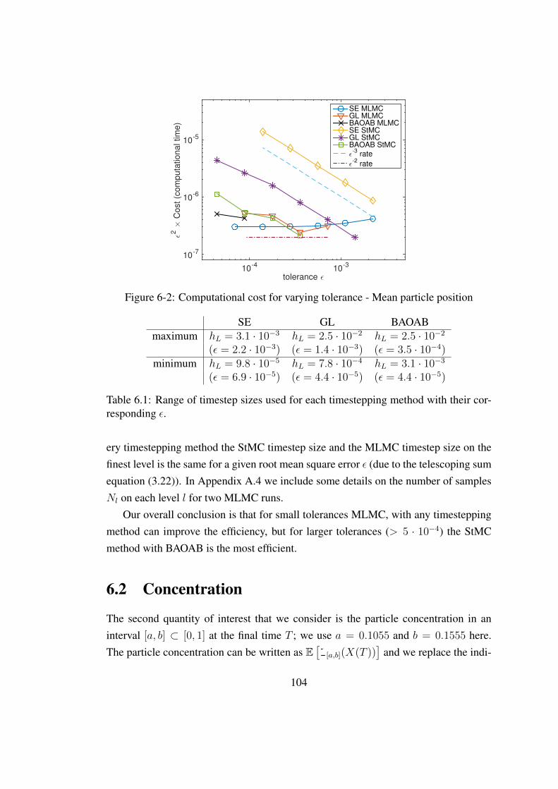
tolerance ǫ10

-410

-3

ǫ2 ×

Cost

(com

puta

tio

nal tim

e)

10-7

10-6

10-5

SE MLMCGL MLMCBAOAB MLMCSE StMCGL StMCBAOAB StMC

ǫ-3

rate

ǫ-2

rate

Figure 6-2: Computational cost for varying tolerance - Mean particle position

SE GL BAOABmaximum hL = 3.1 · 10−3 hL = 2.5 · 10−2 hL = 2.5 · 10−2

(ε = 2.2 · 10−3) (ε = 1.4 · 10−3) (ε = 3.5 · 10−4)minimum hL = 9.8 · 10−5 hL = 7.8 · 10−4 hL = 3.1 · 10−3

(ε = 6.9 · 10−5) (ε = 4.4 · 10−5) (ε = 4.4 · 10−5)

Table 6.1: Range of timestep sizes used for each timestepping method with their cor-responding ε.

ery timestepping method the StMC timestep size and the MLMC timestep size on thefinest level is the same for a given root mean square error ε (due to the telescoping sumequation (3.22)). In Appendix A.4 we include some details on the number of samplesNl on each level l for two MLMC runs.

Our overall conclusion is that for small tolerances MLMC, with any timesteppingmethod can improve the efficiency, but for larger tolerances (> 5 · 10−4) the StMCmethod with BAOAB is the most efficient.

6.2 Concentration

The second quantity of interest that we consider is the particle concentration in aninterval [a, b] ⊂ [0, 1] at the final time T ; we use a = 0.1055 and b = 0.1555 here.The particle concentration can be written as E

[1[a,b](X(T ))

]and we replace the indi-

104

cator function with a smoothing polynomial P r,δ[a,b](X(T )) as discussed in Section 5.4.

Firstly, we check the sensitivity on the smoothing parameters δ and r and then presentsome similar experiments as for the mean particle position case.

6.2.1 Sensitivity to smoothing parameters

As discussed in Section 5.4, using the indicator function as a quantity of interest causesa decrease in the MLMC variance rate so we replace it with the smoothing polyno-mial P r,δ

[a,b](X(T )) defined in equation (5.76). In Figures 6-3a and 6-3b we firstly plotV ar[Yl] as a function of the timestep size hl for GL and SE methods to verify condition(iii) of Theorem 3.1. In both plots we use δ = 0.1, three different values of r and thequantity of interest is P r,δ

[a,b](X(T )). We also plot results for the indicator function 1[a,b]

to see how the variances compare. In all cases the tolerance on the root mean square isε = 10−3 and since the SE method has a larger bias error compared to GL we must usea smaller finest timestep size. We do not include any results for BAOAB since they arevery similar to those of GL. We observe that for the smoothed polynomials the vari-ance decays with a quadratic rate and for the non-smooth indicator function the rateis linear as in Figure 5-7. Therefore, Theorem 3.1 holds numerically when using anyof the smoothed polynomials and the cost rate is expected to improve asymptotically.Note however that we do not study how the overall cost (i.e. the constants in equations(3.20) and (3.24)) is affected by this change but as we see later the asymptotic cost rateof MLMC will improve. Also, note that the absolute value of the variance grows as rincreases which is expected since P r,δ

[a,b] converges to the non-smooth indicator functionas r →∞.

In Section 5.4.2 we presented some analysis regarding the errors introduced bythe smoothing polynomial technique. We concluded that as δ → 0 or r → ∞ thesmoothing errors are decreasing.

Since we now have to choose a pair of values of δ and r for our numerical ex-periments we must show that for those values the additional error which is intro-duced by replacing the indicator function by P r,δ

[a,b](X(T )) is indeed small. In Table6.2 (Katsiolides et al., 2018) we present some estimates of the expected values of1[a,b] and of P r,δ

[a,b] for different values of r and a fixed δ = 0.1. The timestep sizeh is such that the bias error is less than ε/

√2 with ε = 10−3 and we also choose

a large number of samples such that the standard deviation of each estimator is less

105

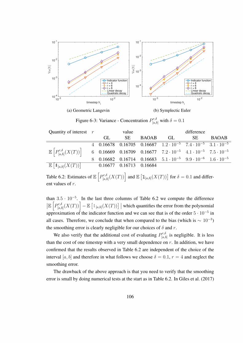
timestep hl

10-3

10-2

Var[Yl]

10-4

10-3

10-2

10-1

Indicator functionr = 4r = 6r = 8Linear decayQuadratic decay

(a) Geometric Langevin

timestep hl

10-3

10-2

Var[Yl]

10-4

10-3

10-2

10-1

Indicator functionr = 4r = 6r = 8Linear decayQuadratic decay

(b) Symplectic Euler

Figure 6-3: Variance - Concentration P r,δ[a,b] with δ = 0.1

Quantity of interest r value differenceGL SE BAOAB GL SE BAOAB

4 0.16678 0.16705 0.16687 1.2 · 10−5 7.4 · 10−5 3.1 · 10−5

E[P r,δ

[a,b](X(T ))]

6 0.16669 0.16709 0.16677 7.2 · 10−5 4.1 · 10−5 7.5 · 10−5

8 0.16682 0.16714 0.16683 5.1 · 10−5 9.9 · 10−6 1.6 · 10−5

E[1[a,b](X(T ))

]0.16677 0.16713 0.16684

Table 6.2: Estimates of E[P r,δ

[a,b](X(T ))]

and E[1[a,b](X(T ))

]for δ = 0.1 and differ-

ent values of r.

than 3.5 · 10−5. In the last three columns of Table 6.2 we compute the difference∣∣E [P r,δ[a,b](X(T ))

]−E

[1[a,b](X(T ))

] ∣∣ which quantifies the error from the polynomialapproximation of the indicator function and we can see that is of the order 5 · 10−5 inall cases. Therefore, we conclude that when compared to the bias (which is ∼ 10−3)the smoothing error is clearly negligible for our choices of δ and r.

We also verify that the additional cost of evaluating P r,δ[a,b] is negligible. It is less

than the cost of one timestep with a very small dependence on r. In addition, we haveconfirmed that the results observed in Table 6.2 are independent of the choice of theinterval [a, b] and therefore in what follows we choose δ = 0.1, r = 4 and neglect thesmoothing error.

The drawback of the above approach is that you need to verify that the smoothingerror is small by doing numerical tests at the start as in Table 6.2. In Giles et al. (2017)

106

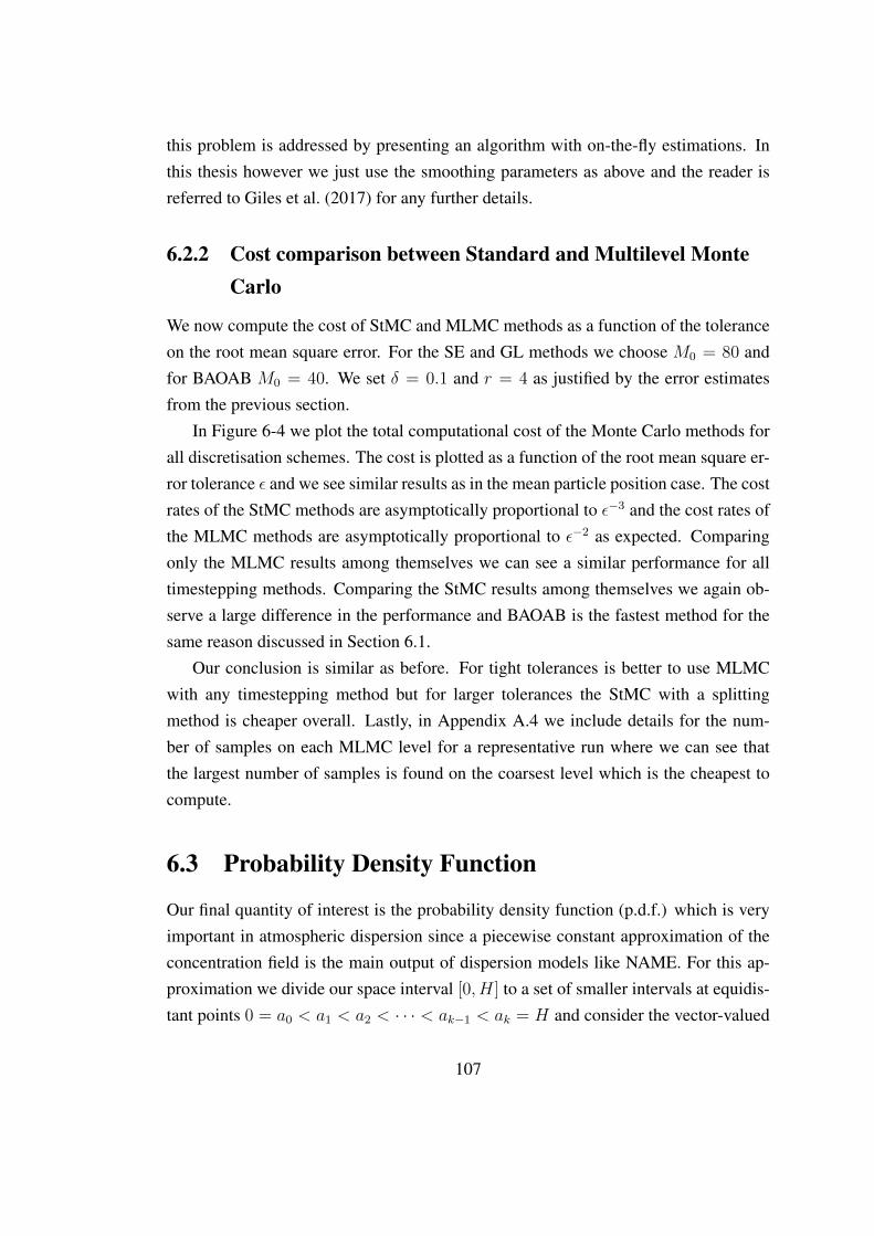
this problem is addressed by presenting an algorithm with on-the-fly estimations. Inthis thesis however we just use the smoothing parameters as above and the reader isreferred to Giles et al. (2017) for any further details.

6.2.2 Cost comparison between Standard and Multilevel MonteCarlo

We now compute the cost of StMC and MLMC methods as a function of the toleranceon the root mean square error. For the SE and GL methods we choose M0 = 80 andfor BAOAB M0 = 40. We set δ = 0.1 and r = 4 as justified by the error estimatesfrom the previous section.

In Figure 6-4 we plot the total computational cost of the Monte Carlo methods forall discretisation schemes. The cost is plotted as a function of the root mean square er-ror tolerance ε and we see similar results as in the mean particle position case. The costrates of the StMC methods are asymptotically proportional to ε−3 and the cost rates ofthe MLMC methods are asymptotically proportional to ε−2 as expected. Comparingonly the MLMC results among themselves we can see a similar performance for alltimestepping methods. Comparing the StMC results among themselves we again ob-serve a large difference in the performance and BAOAB is the fastest method for thesame reason discussed in Section 6.1.

Our conclusion is similar as before. For tight tolerances is better to use MLMCwith any timestepping method but for larger tolerances the StMC with a splittingmethod is cheaper overall. Lastly, in Appendix A.4 we include details for the num-ber of samples on each MLMC level for a representative run where we can see thatthe largest number of samples is found on the coarsest level which is the cheapest tocompute.

6.3 Probability Density Function

Our final quantity of interest is the probability density function (p.d.f.) which is veryimportant in atmospheric dispersion since a piecewise constant approximation of theconcentration field is the main output of dispersion models like NAME. For this ap-proximation we divide our space interval [0, H] to a set of smaller intervals at equidis-tant points 0 = a0 < a1 < a2 < · · · < ak−1 < ak = H and consider the vector-valued

107

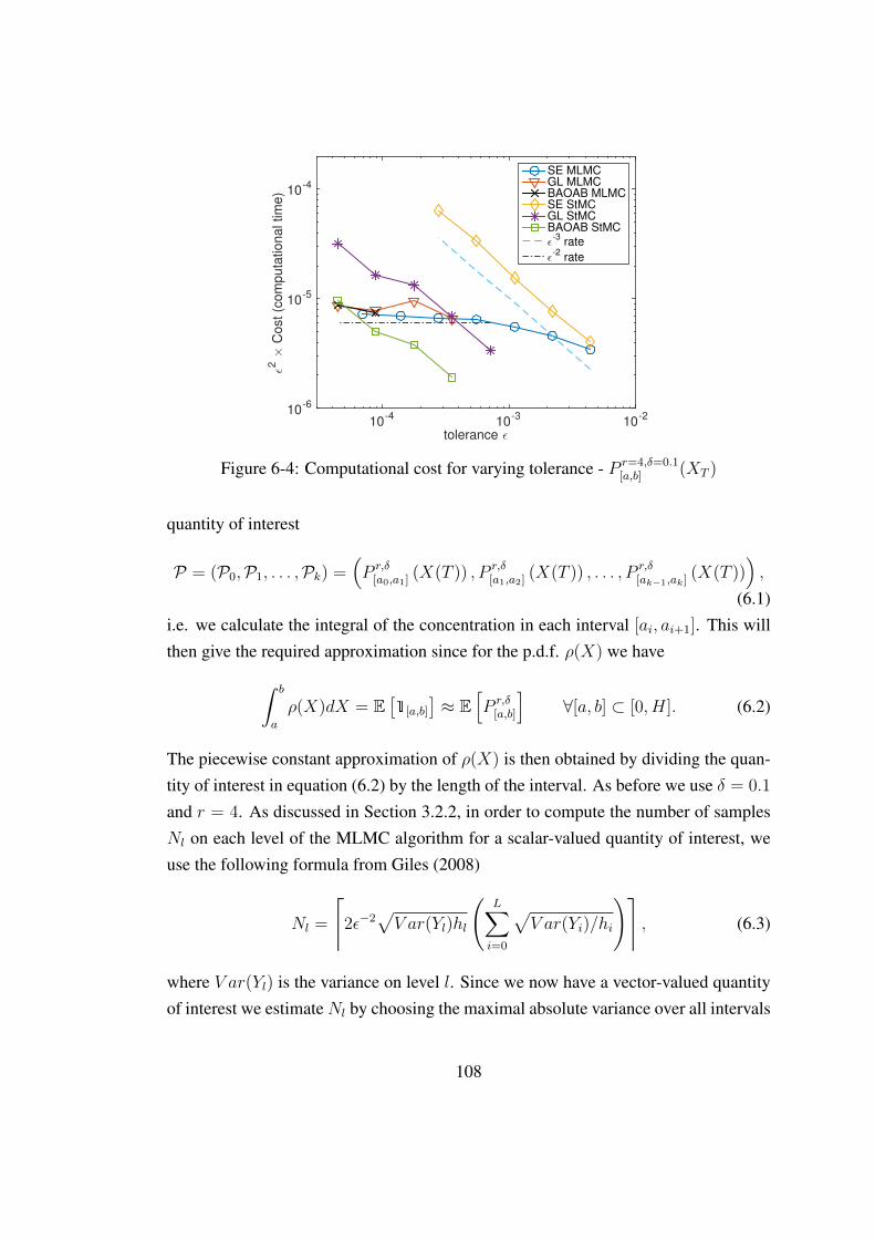
tolerance ǫ10

-410

-310

-2

ǫ2 ×

Cost

(com

puta

tio

nal tim

e)

10-6

10-5

10-4

SE MLMCGL MLMCBAOAB MLMCSE StMCGL StMCBAOAB StMC

ǫ-3

rate

ǫ-2

rate

Figure 6-4: Computational cost for varying tolerance - P r=4,δ=0.1[a,b] (XT )

quantity of interest

P = (P0,P1, . . . ,Pk) =(P r,δ

[a0,a1] (X(T )) , P r,δ[a1,a2] (X(T )) , . . . , P r,δ

[ak−1,ak] (X(T ))),

(6.1)i.e. we calculate the integral of the concentration in each interval [ai, ai+1]. This willthen give the required approximation since for the p.d.f. ρ(X) we have∫ b

a

ρ(X)dX = E[1[a,b]

]≈ E

[P r,δ

[a,b]

]∀[a, b] ⊂ [0, H]. (6.2)

The piecewise constant approximation of ρ(X) is then obtained by dividing the quan-tity of interest in equation (6.2) by the length of the interval. As before we use δ = 0.1

and r = 4. As discussed in Section 3.2.2, in order to compute the number of samplesNl on each level of the MLMC algorithm for a scalar-valued quantity of interest, weuse the following formula from Giles (2008)

Nl =

⌈2ε−2

√V ar(Yl)hl

(L∑i=0

√V ar(Yi)/hi

)⌉, (6.3)

where V ar(Yl) is the variance on level l. Since we now have a vector-valued quantityof interest we estimateNl by choosing the maximal absolute variance over all intervals

108

Position(X)0 0.1 0.2 0.3 0.4 0.5

Pro

babili

ty d

ensity

0

0.5

1

1.5

2

2.5

3

3.5

4

4.5

Position(X)0 0.1 0.2 0.3 0.4 0.5

Pro

babili

ty d

ensity

0

0.5

1

1.5

2

2.5

3

3.5

4

4.5

Position(X)0 0.1 0.2 0.3 0.4 0.5

Pro

babili

ty d

ensity

0

0.5

1

1.5

2

2.5

3

3.5

4

4.5

Figure 6-5: Piecewise constant approximation of probability density function for re-lease height 0.05 (top left), 0.10 (top right) and 0.20 (bottom).

(which guarantees that the error is below the tolerance in all intervals). In particular,we let Pl,i = P r,δ

[ai,ai+1](XT,l) and Y0,i = P0,i, Yl,i = Pl,i − Pl−1,i, for l = 1, . . . , L andi = 0, . . . , k − 1. Then, we use max

i=0,...,k−1|V ar(Yl,i)| in place of V ar(Yl) in equation

6.3 (Katsiolides et al., 2018).With the p.d.f. setting as above we can now construct density function plots. In

Figure 6-5 we plot piecewise constant approximations of the p.d.f. of X(T ) usingSymplectic Euler and MLMC with intervals of size 0.05. The plot on the top leftuses X(0) = 0.05 that corresponds to a release height of 50m above ground, whichis the same initial condition used to obtain all results in Sections 6.1 and 6.2. We alsoinclude results for X(0) = 0.1 and X(0) = 0.2 since we found that the computationalcost is very sensitive to the release height. These heights correspond to 100m and200m above ground, respectively. For all release heights the initial velocity is givenby U(0) = 0.1.

In Table 6.3 we present the computational cost in CPU times necessary to compute

109

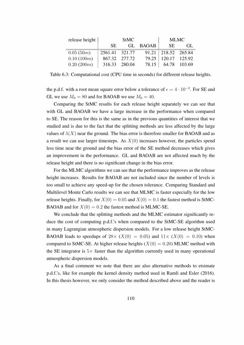
release height StMC MLMCSE GL BAOAB SE GL

0.05 (50m) 2561.41 321.77 91.21 218.52 265.840.10 (100m) 867.32 277.72 79.25 120.17 125.920.20 (200m) 316.33 280.04 78.15 64.78 103.69

Table 6.3: Computational cost (CPU time in seconds) for different release heights.

the p.d.f. with a root mean square error below a tolerance of ε = 4 · 10−3. For SE andGL we use M0 = 80 and for BAOAB we use M0 = 40.

Comparing the StMC results for each release height separately we can see thatwith GL and BAOAB we have a large increase in the performance when comparedto SE. The reason for this is the same as in the previous quantities of interest that westudied and is due to the fact that the splitting methods are less affected by the largevalues of λ(X) near the ground. The bias error is therefore smaller for BAOAB and asa result we can use larger timesteps. As X(0) increases however, the particles spendless time near the ground and the bias error of the SE method decreases which givesan improvement in the performance. GL and BAOAB are not affected much by therelease height and there is no significant change in the bias error.

For the MLMC algorithms we can see that the performance improves as the releaseheight increases. Results for BAOAB are not included since the number of levels istoo small to achieve any speed-up for the chosen tolerance. Comparing Standard andMultilevel Monte Carlo results we can see that MLMC is faster especially for the lowrelease heights. Finally, for X(0) = 0.05 and X(0) = 0.1 the fastest method is StMC-BAOAB and for X(0) = 0.2 the fastest method is MLMC-SE.

We conclude that the splitting methods and the MLMC estimator significantly re-duce the cost of computing p.d.f.’s when compared to the StMC-SE algorithm usedin many Lagrangian atmospheric dispersion models. For a low release height StMC-BAOAB leads to speedups of 28× (X(0) = 0.05) and 11× (X(0) = 0.10) whencompared to StMC-SE. At higher release heights (X(0) = 0.20) MLMC method withthe SE integrator is 5× faster than the algorithm currently used in many operationalatmospheric dispersion models.

As a final comment we note that there are also alternative methods to etsimatep.d.f.’s, like for example the kernel density method used in Ramli and Esler (2016).In this thesis however, we only consider the method described above and the reader is

110

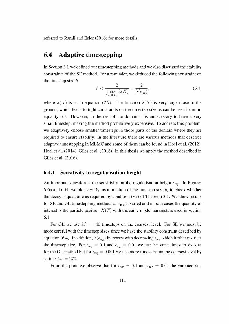
referred to Ramli and Esler (2016) for more details.

6.4 Adaptive timestepping

In Section 3.1 we defined our timestepping methods and we also discussed the stabilityconstraints of the SE method. For a reminder, we deduced the following constraint onthe timestep size h

h <2

maxX∈[0,H]

λ(X)=

2

λ(εreg), (6.4)

where λ(X) is as in equation (2.7). The function λ(X) is very large close to theground, which leads to tight constraints on the timestep size as can be seen from in-equality 6.4. However, in the rest of the domain it is unnecessary to have a verysmall timestep, making the method prohibitively expensive. To address this problem,we adaptively choose smaller timesteps in those parts of the domain where they arerequired to ensure stability. In the literature there are various methods that describeadaptive timestepping in MLMC and some of them can be found in Hoel et al. (2012),Hoel et al. (2014), Giles et al. (2016). In this thesis we apply the method described inGiles et al. (2016).

6.4.1 Sensitivity to regularisation height

An important question is the sensitivity on the regularisation height εreg. In Figures6-6a and 6-6b we plot V ar[Yl] as a function of the timestep size hl to check whetherthe decay is quadratic as required by condition (iii) of Theorem 3.1. We show resultsfor SE and GL timestepping methods as εreg is varied and in both cases the quantity ofinterest is the particle position X(T ) with the same model parameters used in section6.1.

For GL we use M0 = 40 timesteps on the coarsest level. For SE we must bemore careful with the timestep sizes since we have the stability constraint described byequation (6.4). In addition, λ(εreg) increases with decreasing εreg which further restrictsthe timestep size. For εreg = 0.1 and εreg = 0.01 we use the same timestep sizes asfor the GL method but for εreg = 0.001 we use more timesteps on the coarsest level bysetting M0 = 270.

From the plots we observe that for εreg = 0.1 and εreg = 0.01 the variance rate

111

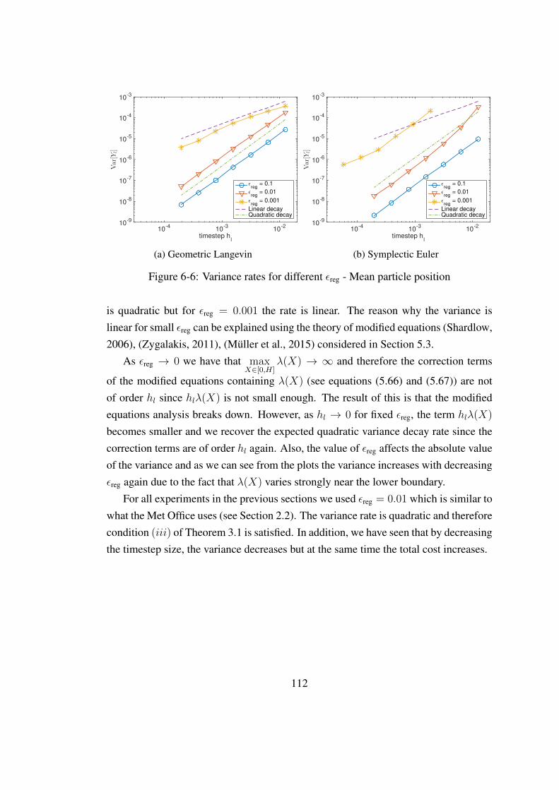
timestep hl

10-4

10-3

10-2

Var[Yl]

10-9

10-8

10-7

10-6

10-5

10-4

10-3

ǫreg

= 0.1

ǫreg

= 0.01

ǫreg

= 0.001

Linear decayQuadratic decay

(a) Geometric Langevin

timestep hl

10-4

10-3

10-2

Var[Yl]

10-9

10-8

10-7

10-6

10-5

10-4

10-3

ǫreg

= 0.1

ǫreg

= 0.01

ǫreg

= 0.001

Linear decayQuadratic decay

(b) Symplectic Euler

Figure 6-6: Variance rates for different εreg - Mean particle position

is quadratic but for εreg = 0.001 the rate is linear. The reason why the variance islinear for small εreg can be explained using the theory of modified equations (Shardlow,2006), (Zygalakis, 2011), (Muller et al., 2015) considered in Section 5.3.

As εreg → 0 we have that maxX∈[0,H]

λ(X) → ∞ and therefore the correction terms

of the modified equations containing λ(X) (see equations (5.66) and (5.67)) are notof order hl since hlλ(X) is not small enough. The result of this is that the modifiedequations analysis breaks down. However, as hl → 0 for fixed εreg, the term hlλ(X)

becomes smaller and we recover the expected quadratic variance decay rate since thecorrection terms are of order hl again. Also, the value of εreg affects the absolute valueof the variance and as we can see from the plots the variance increases with decreasingεreg again due to the fact that λ(X) varies strongly near the lower boundary.

For all experiments in the previous sections we used εreg = 0.01 which is similar towhat the Met Office uses (see Section 2.2). The variance rate is quadratic and thereforecondition (iii) of Theorem 3.1 is satisfied. In addition, we have seen that by decreasingthe timestep size, the variance decreases but at the same time the total cost increases.

112

6.4.2 Adaptive timestepping

Our adaptive MLMC method is as described in Giles et al. (2016) and we adjust thetimestep size at every time tn such that the method is stable. In particular, we use

h(adaptive)n := min

h,λ(Xadapt)

λ(Xn)h

, (6.5)

where Xn is the current particle position and Xadapt is a reference height. With thischoice of adaptive timestep we then have

h(adaptive)n λ(Xn) < λ(Xadapt)h, (6.6)

so if we pick a value for the maximal timestep h andXadapt such that λ(Xadapt)h < 2 wethen guarantee the stability of the SE method (see inequality (6.4)). A very importantobservation about this method of adaptive timestepping is that it is independent of theMLMC level and therefore the telescoping sum in equation (3.22) is not violated whichmeans that it does not introduce any additional bias (Giles et al., 2016).

Now since λ(X) is a decreasing function we only change the timestep size whenthe particles are below the height Xadapt. Note however that although the producth

(adaptive)n λ(Xn) is always bounded such that the SE method is stable, we still need

to regularise λ(X) as in Section 2.2. This is because without regularisation we haveλ → ∞ near the ground which implies that h(adaptive)

n → 0 and therefore it can take aninfinite amount of time to calculate just one trajectory since the number of timestepsmight not be bounded..

As we explain below, when using adaptivity, the fine and coarse steps are not nec-essarily nested as in the uniform timestepping (two fine steps correspond to one coarsestep) and it is possible to have more than two steps on the fine level corresponding toone step on the coarse level. Details of the adaptive MLMC algorithm for the Eulermethod can be found in Giles et al. (2016) and here we only give some details forhow to construct the random increments. In addition, we describe how the boundaryconditions treatment (Section 5.2) can be combined with adaptivity as presented inKatsiolides et al. (2018).

On the coarse level, the interval [0, T ] is partitioned into small sub-intervals throughthe points t(c)i and one step of the numerical method calculates the solution at time t(c)i ,given the solution at time t(c)i−1. Similarly, on the fine level, the interval [0, T ] is divided

113

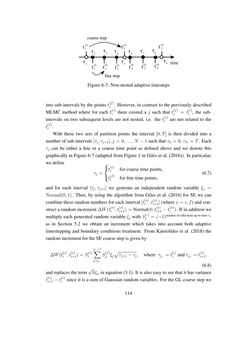
Figure 6-7: Non-nested adaptive timesteps

into sub-intervals by the points t(f)i . However, in contrast to the previously described

MLMC method where for each t(c)i there existed a j such that t(f)j = t

(c)i , the sub-

intervals on two subsequent levels are not nested, i.e. the t(c)i are not related to thet(f)i .

With these two sets of partition points the interval [0, T ] is then divided into anumber of sub-intervals [τj, τj+1], j = 0, . . . , N − 1 such that τ0 = 0, τN = T . Eachτj can be either a fine or a coarse time point as defined above and we denote thisgraphically in Figure 6-7 (adapted from Figure 1 in Giles et al. (2016)). In particular,we define

τj =

t(c)i for coarse time points,

t(f)i for fine time points,

(6.7)

and for each interval [τj, τj+1] we generate an independent random variable ξj ∼Normal(0, 1). Then, by using the algorithm from Giles et al. (2016) for SE we cancombine these random numbers for each interval [t

(x)i , t

(x)i+1] (where x = c, f ) and con-

struct a random increment ∆W (t(x)i , t

(x)i+1) ∼ Normal(0, t(x)

i+1 − t(x)i ). If in addition we

multiply each generated random variable ξj with S(·)j = (−1)number of reflections up to time τj

as in Section 5.2 we obtain an increment which takes into account both adaptivetimestepping and boundary conditions treatment. From Katsiolides et al. (2018) therandom increment for the SE coarse step is given by

∆W (t(c)i , t

(c)i+1) = S

(c)i

j+−1∑j=j−

S(f)j ξj

√τj+1 − τj, where τj− = t

(c)i and τj+ = t

(c)i+1,

(6.8)and replaces the term

√hξn in equation (3.1). It is also easy to see that it has variance

t(c)i+1 − t

(c)i since it is a sum of Gaussian random variables. For the GL coarse step we

114

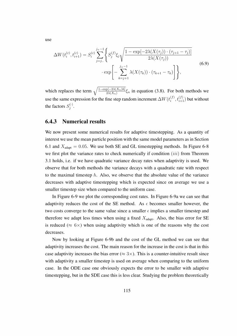
use

∆W (t(c)i , t

(c)i+1) = S

(c)i

j+−1∑j=j−

S

(f)j ξj

√1− exp[−2λ(X(τj)) · (τj+1 − τj)]

2λ(X(τj))

· exp

[−

j+−1∑k=j+1

λ(X(τk)) · (τk+1 − τk)

],

(6.9)

which replaces the term√

1−exp[−2λ(Xn)h]2λ(Xn)

ξn in equation (3.8). For both methods we

use the same expression for the fine step random increment ∆W (t(f)i , t

(f)i+1) but without

the factors S(·)j .

6.4.3 Numerical results

We now present some numerical results for adaptive timestepping. As a quantity ofinterest we use the mean particle position with the same model parameters as in Section6.1 and Xadapt = 0.05. We use both SE and GL timestepping methods. In Figure 6-8we first plot the variance rates to check numerically if condition (iii) from Theorem3.1 holds, i.e. if we have quadratic variance decay rates when adaptivity is used. Weobserve that for both methods the variance decays with a quadratic rate with respectto the maximal timestep h. Also, we observe that the absolute value of the variancedecreases with adaptive timestepping which is expected since on average we use asmaller timestep size when compared to the uniform case.

In Figure 6-9 we plot the corresponding cost rates. In Figure 6-9a we can see thatadaptivity reduces the cost of the SE method. As ε becomes smaller however, thetwo costs converge to the same value since a smaller ε implies a smaller timestep andtherefore we adapt less times when using a fixed Xadapt. Also, the bias error for SEis reduced (≈ 6×) when using adaptivity which is one of the reasons why the costdecreases.

Now by looking at Figure 6-9b and the cost of the GL method we can see thatadaptivity increases the cost. The main reason for the increase in the cost is that in thiscase adaptivity increases the bias error (≈ 3×). This is a counter-intuitive result sincewith adaptivity a smaller timestep is used on average when comparing to the uniformcase. In the ODE case one obviously expects the error to be smaller with adaptivetimestepping, but in the SDE case this is less clear. Studying the problem theoretically

115

max timestep10

-410

-310

-2

Var[Y

l]

10-9

10-8

10-7

10-6

10-5

10-4

10-3

UniformAdaptiveQuadratic decay

(a) Symplectic Euler

max timestep10

-410

-310

-2

Var[Y

l]

10-9

10-8

10-7

10-6

10-5

10-4

10-3

UniformAdaptiveQuadratic decay

(b) Geometric Langevin

Figure 6-8: Variance rates - Uniform and adaptive timesteps

to see what behaviour we should expect is hard for our non-linear SDE and beyond thescope of this thesis. However, to make sure that there are no bugs in the code we madeseveral tests like for example testing the case when σ = 0. For this ODE we confirmedthat GL reduces the bias error. Further investigation of this problem which might belinked to the divergence of λ(X) near the ground, can be a topic for future research.Also, it will be interesting to see results when using the BAOAB method which can beanother direction for future research.

116

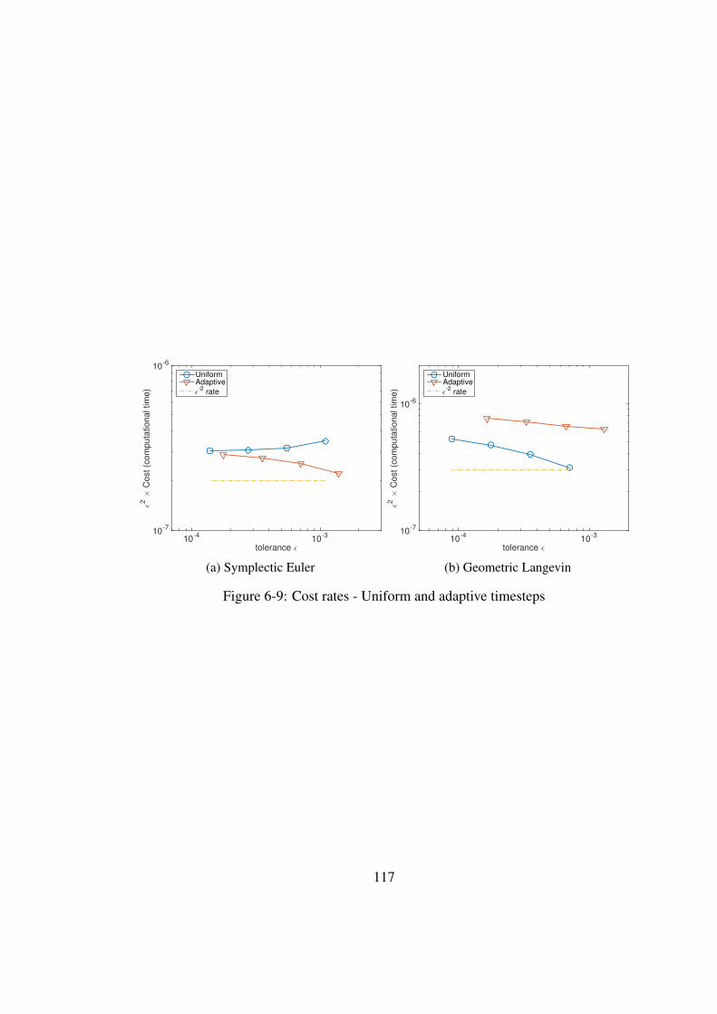
tolerance ǫ10

-410

-3

ǫ2 ×

Co

st

(co

mp

uta

tio

na

l tim

e)

10-7

10-6

UniformAdaptive

ǫ-2

rate

(a) Symplectic Euler

tolerance ǫ10

-410

-3

ǫ2 ×

Co

st

(co

mp

uta

tio

na

l tim

e)

10-7

10-6

UniformAdaptive

ǫ-2

rate

(b) Geometric Langevin

Figure 6-9: Cost rates - Uniform and adaptive timesteps

117

Chapter 7

Higher Dimensional Models

After presenting theoretical and numerical results for the one-dimensional models wenow study higher dimensional models which give a better description of the atmo-spheric conditions since turbulence is not just one-dimensional. In a realistic modelfor the transport and spread of particles in the atmosphere there are two main thingshappening: Firstly, the particles are advected by a background velocity field, which atthe Met Office is obtained from the numerical forecast model. However, this field hasa finite resolution, so can only represent eddies which are larger than some cutoff Λ.Secondly, any processes at scales below this cutoff are modelled by the turbulent com-ponent U(t) of the particles’ velocity. In the model, this is described by the randomterms.

Based on the above two properties, we construct a set of synthetic backgroundvelocity fields and study the transport and spread of particles in those fields. The back-ground velocity field is constructed as a sum of modes with the correct energy spectrumand is such that it is non-divergent in order to avoid the unphysical accumulation ofparticles in some parts of the domain. The non-divergent property was also one of thereasons that we did not consider a background velocity in the one-dimensional casesince this would require a constant vertical quantity in the entire boundary layer whichis not physical. Lastly, the parameters of the turbulence model are adjusted such thatthey correctly represent the unresolved processes at the scales below the cutoff Λ.

Our models have the general form given in the Introduction by equations (1.1)and (1.2) for d = 2 and d = 3. For d = 2 the model will describe horizontal two-dimensional homogeneous turbulence. Since the atmospheric boundary layer is very

118

thin when you consider a global scale, this model can be a good approximation andtherefore we study it first. For d = 3 the model will combine the horizontal structureof the homogeneous two-dimensional model with the vertical structure of the inhomo-geneous one-dimensional model intoduced in Section 2.1. In Sections 7.1 and 7.2 westudy the two- and three-dimensional models respectively and we present some nu-merical results to compare the efficiency of Standard and Multilevel Monte Carlo withthe Symplectic Euler method. Finally, in Section 7.3 we study the effect on the perfor-mance when we change some of the model parameters and we present some numericalresults with the BAOAB method.

All numerical results in this chapter were generated with an updated version ofthe C++ code used in Chapter 6. The code can be downloaded freely under the GPLlicense from https://bitbucket.org/em459/mlmclangevin.

7.1 Two-dimensional model for homogeneousturbulence

Our two-dimensional model describes homogeneous turbulence on the horizontal planeand U(t) = (U1(t), U2(t)), X(t) = (X1(t), X2(t)) denote the two-dimensional veloc-ity and position respectively. The model is given by the following SDEs

dUi(t) = −Ui(t)τ

dt+

√2σ2

U

τdWi(t), (7.1)

dXi(t) = (vi(X(t), t) + Ui(t)) dt, i = 1, 2, (7.2)

which are a special case of the general model given by equations (1.1) and (1.2) withd = 2. W1(t) and W2(t) are independent Brownian motions and we assume that thereare no boundary conditions so that the particles can travel anywhere.

Since the turbulence is homogeneous, τ (velocity decorrelation timescale) and σ2U

(variance at equilibrium) are constants and we also assume that they are isotropic (i.e.the same in all directions). Equation (7.1) can therefore be seen as a higher dimensionalextension of the one-dimensional homogeneous model described by equation (2.13).τ and σU could be different in each direction and also depend on X = (X1, X2) butfor simplicity we do not consider any of these cases. The reader can refer to Websteret al. (2003) for more information on how these functions are chosen for practical

119

applications. We define τ and σU in Section 7.1.2. Also note that in the most generalcase we could have something like

dUi(t) = −d∑j=1

AijUj(t)dt+d∑j=1

BijdWj(t),

for some non-diagonal matrices A and B. However, in our models we assume that thematrices A and B are diagonal and studying this more general model would be out ofthe scope of this thesis.

In contrast to the model in the previous chapter, the background velocity field(v1(X(t), t), v2(X(t), t)) is non-zero and in the higher dimensional cases we studyhow it affects the Monte Carlo results. In Section 7.1.1 we define the backgroundvelocity field as described in Fung and Vassilicos (1998) and Thomson and Devenish(2005).

Finally, we define our initial conditions. In the one-dimensional case we useddeterministic initial conditions but for higher dimensional models we study randominitial conditions. The reason why we choose random initial conditions is due to thefact that the background velocity is non-zero and we assume that the initial velocityadapts to the ambient velocity of the flow when the particles are released. In particular,we use X(0) = (0, 0) and U(0) = (U1(0), U2(0)) with U1(0), U2(0) independent anddistributed as Normal(0, σ2

U).

7.1.1 The background velocity field

Our background velocity field v(X, t) = (v1(X, t), v2(X, t)) describes the wind fieldas a sum of modes, each with a characteristic length scale Li and associated wavenum-ber ki = 2π/Li. The modes have length scales between Λ (the grid size of the weatherforecast model) and L (the largest scale, which is of order of the radius of the Earth)and the kinetic energy carried by each of them should be consistent with the energycarried in the real atmosphere. From Nastrom and Gage (1985) the energy spectrumin the atmosphere is given by

E(k) = E0L(kL)−p with 1 ≤ p ≤ 3, (7.3)

120

for some constant E0, which means that the energy carried by modes in the range[ka, . . . , kb] is given by ∫ kb

ka

E(k)dk. (7.4)

In addition, the background velocity field should be divergence free.These lead to the following function from Fung and Vassilicos (1998) and Thom-

son and Devenish (2005)

v(X, t) =N∑n=1

[An cos(kn ·X + ωnt) + Bn sin(kn ·X + ωnt)] , (7.5)

which can also be written in complex form as

v(X, t) =N∑n=1

[An Re(gn) + Bn Im(gn)] , (7.6)

where gn = cos(kn ·X + ωnt) + i sin(kn ·X + ωnt). Here, N is the number of modesand for each n we compute a random unit vector n and set kn = knn where

kn = kLan−1 with a =

(L

Λ

) 1N−1

. (7.7)

The vector kn is the wavenumber vector of the nth mode, kL = 2πL

, L is the size ofthe largest eddy and Λ is the size of the smallest eddy which can be represented by thenumerical weather forecast model, i.e. the grid resolution.

The vectors An and Bn are the mode amplitudes and since we require that thebackground velocity is incompressible, i.e. ∇·v = 0, it is sufficient to have kn ·An =

kn ·Bn = 0. Therefore, An and Bn are chosen to be random but perpendicular to kn.Their length is given by

|An|2 = |Bn|2 = 2E(kn)∆kn, (7.8)

121

where E(k) is a kinetic energy spectrum and ∆kn is defined by

∆kn =

k2−k1

2for n = 1,

kn+1−kn−1

2for 2 ≤ n ≤ N − 1,

kN−kN−1

2for n = N.

(7.9)

Lastly, as in Fung and Vassilicos (1998) we set ωn (the frequency of the nth mode)to be proportional to the inverse eddy turnover time and use

ωn = C√k3nE(kn), (7.10)

where C is a dimensionless constant of proportionality. Equation (7.10) was used forexperiments in Fung and Vassilicos (1998) and Thomson and Devenish (2005). InFung and Vassilicos (1998) they also study the case when ωn = Ukn with a constantvelocity U and in Thomson and Devenish (2005) they also consider a stationary fieldwith ωn = 0. In this thesis we only consider equation (7.10).

7.1.2 σU and τ

We now define σU and τ which are the last two components to complete our model.The constant σU is chosen such that the total kinetic energy carried by the turbulentmodes (which are represented by the random part of the SDE) is equal to the kineticenergy of the unresolved modes whose wavenumber vector modulus is greater than 2π

Λ.

It is then given by

σ2U =

∫ ∞2πΛ

E(k)dk, (7.11)

where E(k) is the kinetic energy spectrum given by equation (7.3). This integral eval-uates to

σ2U = E0

∫ ∞2πL/Λ

(kL)−pd(kL) = E0z1−p

p− 1

∣∣∣∞2πL/Λ

=(2π)1−p

p− 1E0

(Λ

L

)p−1

. (7.12)

The constant τ is chosen to be proportional to the eddy turnover time at the N th modekN = 2π

Λand is given by

τ =1

C√k3NE(kN)

. (7.13)

122

7.1.3 Model scales

Before presenting any numerical results we first analyse the scales of the model vari-ables as we did in Section 2.1.2 for the one-dimensional model. For a physical quantityα we consider a reference scale αref and write

α = αrefα, (7.14)

where α is the corresponding dimensionless parameter. In particular, we consider areference length Lref, a reference time T ref and a reference speed U ref. These threequantities are related by (see Section 2.1.2)

Lref = U refT ref. (7.15)

For the physical values X,U, L,Λ and t we then have

X = LrefX, U = U refU, L = LrefL, Λ = LrefΛ, t = T reft, (7.16)

where X, U, L, Λ and t are the dimensionless parameters.We set Lref = 1km = 1000m and we determine U ref by considering E0 in equation

(7.3). Since the energy E(k)dk of a unit particle has the dimension of a squaredvelocity we have that E0 has the same dimension which implies that

E0 = (U ref)2E0. (7.17)

Using this equation, we fix U ref such that E0 = 1 which gives

E0 = (U ref)2. (7.18)

If we now find the physical value of E0 we can then compute U ref. In order to find thisvalue we use Figure 4 from Nastrom and Gage (1985) where we obtainE(10−5m−1) ≈106m3s−2. Later, in our numerical results we use L = 1000km = 106m and p = 5

3so

using equation (7.3) givesE0 ≈ 10

53m2s−2. (7.19)

123

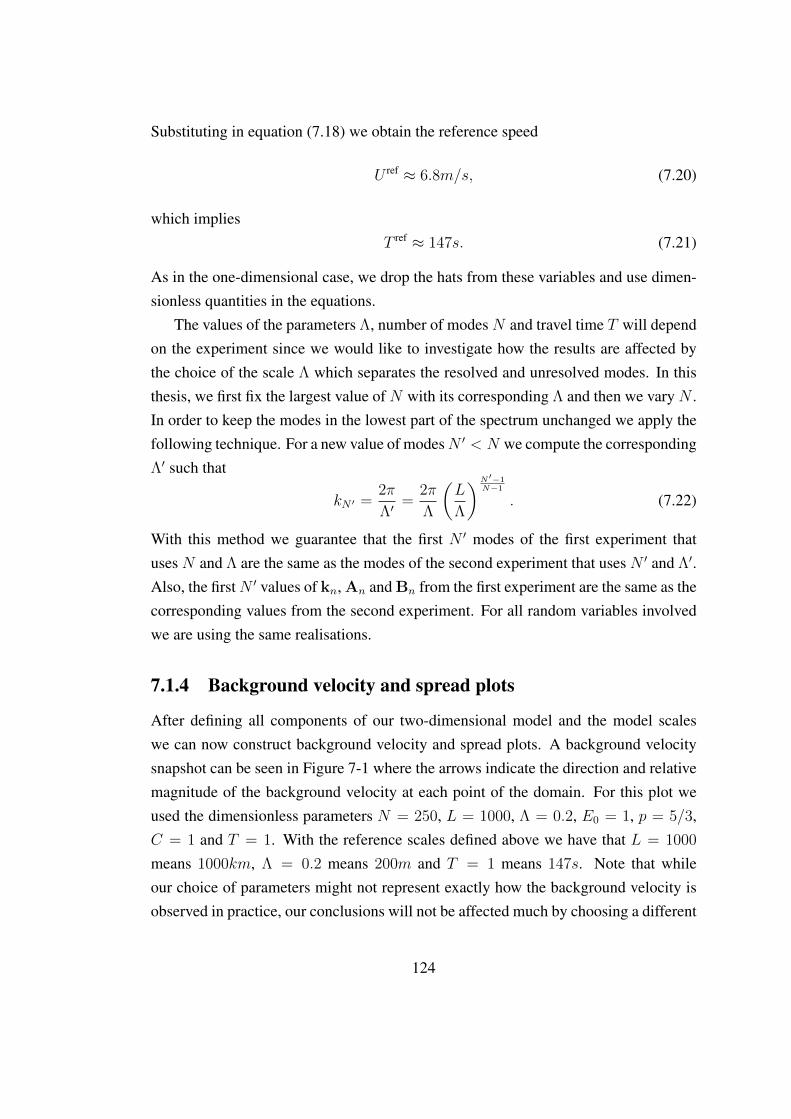
Substituting in equation (7.18) we obtain the reference speed

U ref ≈ 6.8m/s, (7.20)

which impliesT ref ≈ 147s. (7.21)

As in the one-dimensional case, we drop the hats from these variables and use dimen-sionless quantities in the equations.

The values of the parameters Λ, number of modes N and travel time T will dependon the experiment since we would like to investigate how the results are affected bythe choice of the scale Λ which separates the resolved and unresolved modes. In thisthesis, we first fix the largest value of N with its corresponding Λ and then we vary N .In order to keep the modes in the lowest part of the spectrum unchanged we apply thefollowing technique. For a new value of modesN ′ < N we compute the correspondingΛ′ such that

kN ′ =2π

Λ′=

2π

Λ

(L

Λ

)N′−1N−1

. (7.22)

With this method we guarantee that the first N ′ modes of the first experiment thatuses N and Λ are the same as the modes of the second experiment that uses N ′ and Λ′.Also, the firstN ′ values of kn, An and Bn from the first experiment are the same as thecorresponding values from the second experiment. For all random variables involvedwe are using the same realisations.

7.1.4 Background velocity and spread plots

After defining all components of our two-dimensional model and the model scaleswe can now construct background velocity and spread plots. A background velocitysnapshot can be seen in Figure 7-1 where the arrows indicate the direction and relativemagnitude of the background velocity at each point of the domain. For this plot weused the dimensionless parameters N = 250, L = 1000, Λ = 0.2, E0 = 1, p = 5/3,C = 1 and T = 1. With the reference scales defined above we have that L = 1000

means 1000km, Λ = 0.2 means 200m and T = 1 means 147s. Note that whileour choice of parameters might not represent exactly how the background velocity isobserved in practice, our conclusions will not be affected much by choosing a different

124

X1

-20 -10 0 10 20

X2

-25

-20

-15

-10

-5

0

5

10

15

20

25

Figure 7-1: A background velocity field snapshot for two-dimensional turbulence.

set of parameters.Next, we study the spread of the plume with respect to the travel time T . With a

non-zero background velocity field we expect the particles to be spread by two pro-cesses: (a) turbulence described by the stochastic part of the SDEs and (b) particlesgetting caught up in different eddies of the background velocity field. Since the parti-cles are initially close together, we expect the effect of (a) to dominate for small timesand the effect of (b) to dominate for large times. Our aim for the rest of this sectionis to determine at what times these different processes dominate, in order to study theperformance of MLMC in those very different regimes.

Mathematically the spread is described by the standard deviation of the particle’sposition, which is estimated using

s =

√√√√ 1

NL − 1

NL∑j=1

[(X1

(j)ML− µ1

)2

+(X2

(j)ML− µ2

)2], (7.23)

where

µi =1

NL

NL∑j=1

Xi(j)ML, i = 1, 2, (7.24)

is an estimate for the mean particle position. The value Xi(j)ML

is an approximation ofthe jth independent sample path of Xi(T ) using some timestepping method with ML

125

timesteps.For the one-dimensional homogeneous model with zero background velocity stud-

ied in Section 2.1.1 (equations (2.13) and (2.8)) it is possible to derive an exact expres-sion for the spread s. Details of the derivation can be found in Appendix A.2.2 fromwhich we obtain

s ∼

t for t τ,√t for t τ,

for stochastic U(0) ∼ Normal(0, σ2U) and

s ∼

t32 for t τ,√t for t τ,

for constant U(0). The same behaviour can also be obtained theoretically for a two-dimensional homogeneous model with zero background velocity (i.e. v = 0 in equa-tions (7.1) and (7.2)). The result for stochastic U(0) agrees with the analysis fromTaylor (1921) and the short time behaviour for constant U(0) agrees with Richard-son’s t3 law for s2.

For the two-dimensional model described by equations (7.1) and (7.2) with non-zero background velocity it is difficult to obtain a theoretical expression for the spreadso we just approximate it numerically. However, for small travel times we expect asimilar behaviour as in the case of a zero background velocity (since the particles havenot been separated in different eddies yet) and for large travel times we expect a furtherincrease in the particle spread.

In Figure 7-2 we plot the spread with respect to time T for random and constantU(0) using the Symplectic Euler method. The plots contain data for three differentvalues of N (and also different Λ as discussed at the end of Section 7.1.3) and thesolid vertical lines indicate the value of τ that corresponds to each value of N . Thehorizontal dotted lines represent the value of 2Λ since we are interested to see at whattimes the spread becomes larger than 2Λ where Λ is the radius of the smallest eddycorresponding to each number of modes N .

For random U(0) the rate is initially linear and for constant U(0) it is initiallyproportional to t

32 . Therefore, the short time behaviour agrees with the theoretical

results of the simpler problem considered in Appendix A.2.2. After approximatelytime τ (which depends on Λ as can be seen from equation (7.13)) the behaviour for

126

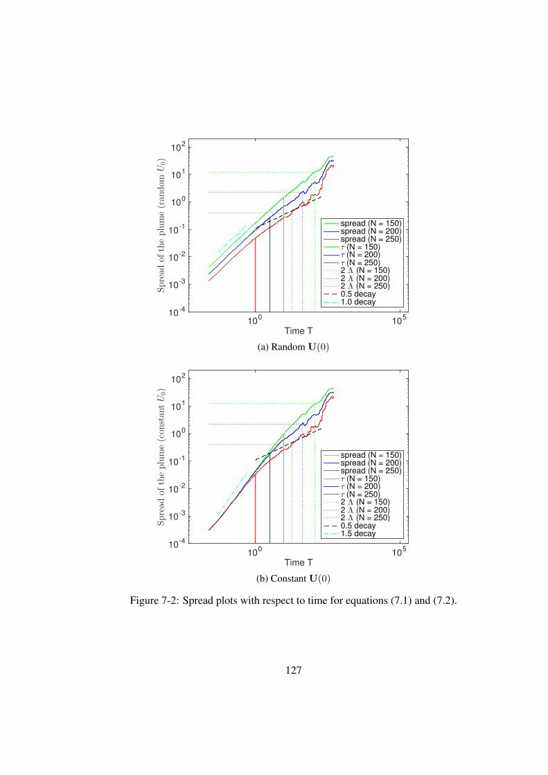
Time T10

010

5

Spread

oftheplume(ran

dom

U0)

10-4

10-3

10-2

10-1

100

101

102

spread (N = 150)spread (N = 200)spread (N = 250)τ (N = 150)τ (N = 200)τ (N = 250)2 Λ (N = 150)2 Λ (N = 200)2 Λ (N = 250)0.5 decay1.0 decay

(a) Random U(0)

Time T10

010

5

Spread

oftheplume(con

stan

tU0)

10-4

10-3

10-2

10-1

100

101

102

spread (N = 150)spread (N = 200)spread (N = 250)τ (N = 150)τ (N = 200)τ (N = 250)2 Λ (N = 150)2 Λ (N = 200)2 Λ (N = 250)0.5 decay1.5 decay

(b) Constant U(0)

Figure 7-2: Spread plots with respect to time for equations (7.1) and (7.2).

127

both initial conditions is similar. We observe that for N = 250 and N = 200 the ratebecomes proportional to the square root of t.

For very large values of T the rate becomes linear again and it is also noisy as it canbe seen from the plot. The reason that it becomes linear is due to the fact that for largetimes T the particles are separated in different eddies of the background velocity fieldwhich causes an increase in the rate. This separation is expected to happen at timeswhen the spread exceeds the value 2Λ (since Λ is the radius of the smallest eddy)which is also the case (approximately) for our model as it can be seen from the plot.For N = 150 the rate only becomes linear after time τ .

7.1.5 Numerical results

In this section we present some Monte Carlo results in a similar way as in Chapter 6for the one-dimensional model. We approximate the solution of the two-dimensionalmodel given by equations (7.1) and (7.2) with τ , σU and v(X, t) as in equations (7.13),(7.11) and (7.5) respectively. The model parameters areN = 250, L = 1000, Λ = 0.2,E0 = 1, p = 5/3 and C = 1. For initial conditions we use X(0) = (0, 0) and U(0) =

(U1(0), U2(0)) with U1(0), U2(0) independent and distributed as Normal(0, σ2U).

Since our model is homogeneous the profiles of σU and τ (see Section 7.1.2) re-main constant and they do not become large as in the one-dimensional inhomogeneousmodel considered in Chapter 6. As a result, we do not expect any large improve-ments in the Monte Carlo performance when using Geometric Langevin or BAOABmethods. Therefore, we only consider the Symplectic Euler method which is currentlyused by the Met Office and concentrate on investigating the gains of MLMC comparedto StMC.

In order to choose suitable travel times we use the spread plot given in Figure 7-2a.We consider two travel times, T1 ≈ τ+TΛ

2and T2 ≈ 3

2TΛ where TΛ is defined as the

time when the spread becomes larger than 2Λ. We choose the first time T1 in orderto compare results when the spread is linear and the particles are not yet separatedinto different eddies which means that we are in the regime where the spread is dueto turbulence. The second time T2 > TΛ is chosen in order to study how the MonteCarlo methods are affected when the particles are separated in different eddies (sinceΛ is the radius of the smallest eddy). In particular, when the travel time is larger thanTΛ it might be harder to couple the random variables in the MLMC coarse step since

128

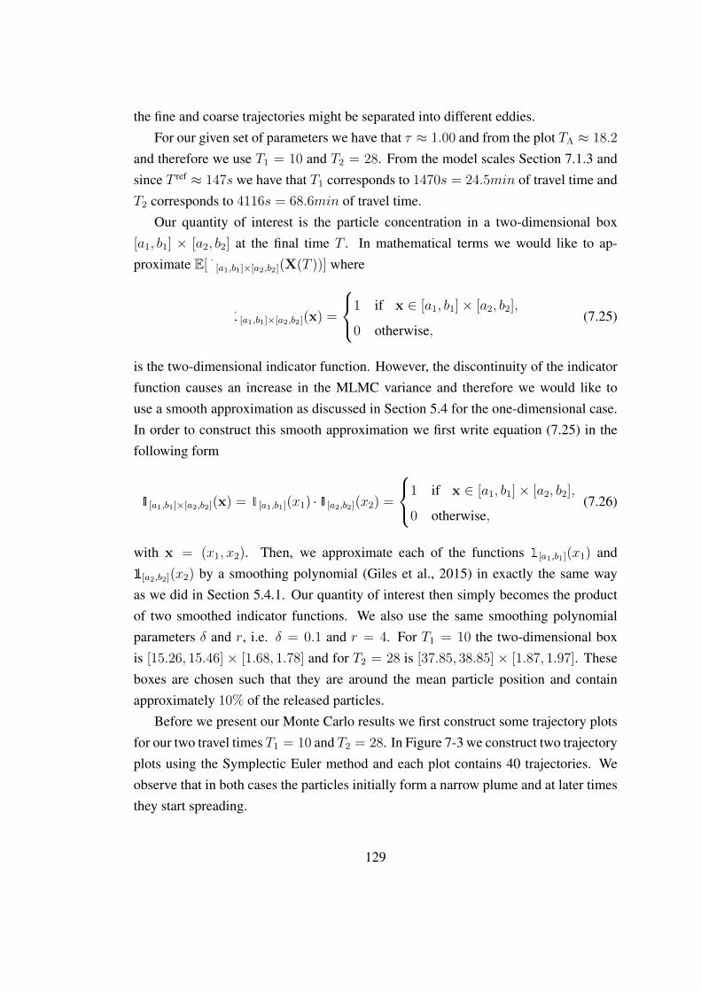
the fine and coarse trajectories might be separated into different eddies.For our given set of parameters we have that τ ≈ 1.00 and from the plot TΛ ≈ 18.2

and therefore we use T1 = 10 and T2 = 28. From the model scales Section 7.1.3 andsince T ref ≈ 147s we have that T1 corresponds to 1470s = 24.5min of travel time andT2 corresponds to 4116s = 68.6min of travel time.

Our quantity of interest is the particle concentration in a two-dimensional box[a1, b1] × [a2, b2] at the final time T . In mathematical terms we would like to ap-proximate E[1[a1,b1]×[a2,b2](X(T ))] where

1[a1,b1]×[a2,b2](x) =

1 if x ∈ [a1, b1]× [a2, b2],

0 otherwise,(7.25)

is the two-dimensional indicator function. However, the discontinuity of the indicatorfunction causes an increase in the MLMC variance and therefore we would like touse a smooth approximation as discussed in Section 5.4 for the one-dimensional case.In order to construct this smooth approximation we first write equation (7.25) in thefollowing form

1[a1,b1]×[a2,b2](x) = 1[a1,b1](x1) ·1[a2,b2](x2) =

1 if x ∈ [a1, b1]× [a2, b2],

0 otherwise,(7.26)

with x = (x1, x2). Then, we approximate each of the functions 1[a1,b1](x1) and1[a2,b2](x2) by a smoothing polynomial (Giles et al., 2015) in exactly the same wayas we did in Section 5.4.1. Our quantity of interest then simply becomes the productof two smoothed indicator functions. We also use the same smoothing polynomialparameters δ and r, i.e. δ = 0.1 and r = 4. For T1 = 10 the two-dimensional boxis [15.26, 15.46] × [1.68, 1.78] and for T2 = 28 is [37.85, 38.85] × [1.87, 1.97]. Theseboxes are chosen such that they are around the mean particle position and containapproximately 10% of the released particles.

Before we present our Monte Carlo results we first construct some trajectory plotsfor our two travel times T1 = 10 and T2 = 28. In Figure 7-3 we construct two trajectoryplots using the Symplectic Euler method and each plot contains 40 trajectories. Weobserve that in both cases the particles initially form a narrow plume and at later timesthey start spreading.

129

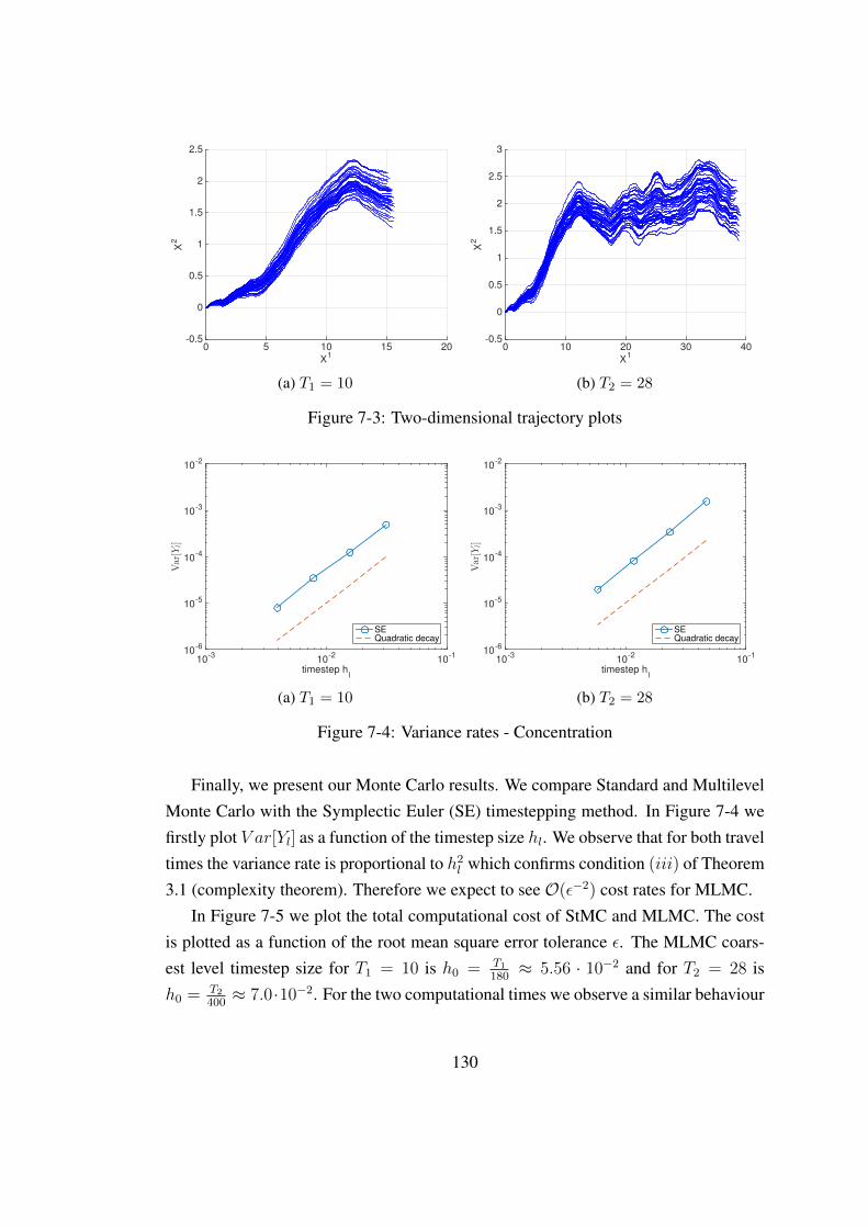
X1

0 5 10 15 20

X2

-0.5

0

0.5

1

1.5

2

2.5

(a) T1 = 10

X1

0 10 20 30 40

X2

-0.5

0

0.5

1

1.5

2

2.5

3

(b) T2 = 28

Figure 7-3: Two-dimensional trajectory plots

timestep hl

10-3

10-2

10-1

Var[Y

l]

10-6

10-5

10-4

10-3

10-2

SEQuadratic decay

(a) T1 = 10

timestep hl

10-3

10-2

10-1

Var[Y

l]

10-6

10-5

10-4

10-3

10-2

SEQuadratic decay

(b) T2 = 28

Figure 7-4: Variance rates - Concentration

Finally, we present our Monte Carlo results. We compare Standard and MultilevelMonte Carlo with the Symplectic Euler (SE) timestepping method. In Figure 7-4 wefirstly plot V ar[Yl] as a function of the timestep size hl. We observe that for both traveltimes the variance rate is proportional to h2

l which confirms condition (iii) of Theorem3.1 (complexity theorem). Therefore we expect to see O(ε−2) cost rates for MLMC.

In Figure 7-5 we plot the total computational cost of StMC and MLMC. The costis plotted as a function of the root mean square error tolerance ε. The MLMC coars-est level timestep size for T1 = 10 is h0 = T1

180≈ 5.56 · 10−2 and for T2 = 28 is

h0 = T2

400≈ 7.0·10−2. For the two computational times we observe a similar behaviour

130

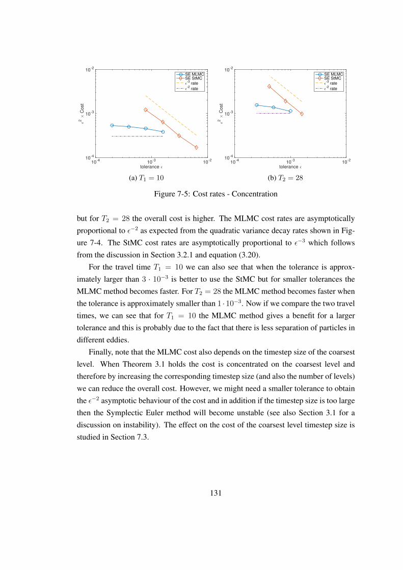
tolerance ǫ

10-4

10-3

10-2

ǫ2 ×

Co

st

10-4

10-3

10-2

SE MLMC

SE StMC

ǫ-3

rate

ǫ-2

rate

(a) T1 = 10

tolerance ǫ

10-4

10-3

10-2

ǫ2 ×

Co

st

10-4

10-3

10-2

SE MLMC

SE StMC

ǫ-3

rate

ǫ-2

rate

(b) T2 = 28

Figure 7-5: Cost rates - Concentration

but for T2 = 28 the overall cost is higher. The MLMC cost rates are asymptoticallyproportional to ε−2 as expected from the quadratic variance decay rates shown in Fig-ure 7-4. The StMC cost rates are asymptotically proportional to ε−3 which followsfrom the discussion in Section 3.2.1 and equation (3.20).

For the travel time T1 = 10 we can also see that when the tolerance is approx-imately larger than 3 · 10−3 is better to use the StMC but for smaller tolerances theMLMC method becomes faster. For T2 = 28 the MLMC method becomes faster whenthe tolerance is approximately smaller than 1 ·10−3. Now if we compare the two traveltimes, we can see that for T1 = 10 the MLMC method gives a benefit for a largertolerance and this is probably due to the fact that there is less separation of particles indifferent eddies.

Finally, note that the MLMC cost also depends on the timestep size of the coarsestlevel. When Theorem 3.1 holds the cost is concentrated on the coarsest level andtherefore by increasing the corresponding timestep size (and also the number of levels)we can reduce the overall cost. However, we might need a smaller tolerance to obtainthe ε−2 asymptotic behaviour of the cost and in addition if the timestep size is too largethen the Symplectic Euler method will become unstable (see also Section 3.1 for adiscussion on instability). The effect on the cost of the coarsest level timestep size isstudied in Section 7.3.

131

7.2 The three-dimensional model

Next, we study a three-dimensional model. For the horizontal direction we assume thatthe motion is described by the two-dimensional model of the previous section with theaddition of vertical wind-shear and for the vertical direction we assume that the motionis described by the model from Chapter 6. In particular, we assume that σU and τ varystrongly with height. In this section we denote by U(t) = (U1(t), U2(t), U3(t)) andX(t) = (X1(t), X2(t), X3(t)) the three-dimensional velocity and position respectively.The first two components denote the horizontal motion and third component denotesthe vertical motion. The model is given by the following SDEs

dUi(t) = −Ui(t)τho

dt+

√2σ2

U,ho

τhodWi(t), (7.27)

dXi(t) = (vi(X(t), t) + Ui(t)) dt, i = 1, 2, (7.28)

dU3(t) = −λ(X3(t))U3(t)dt− ∂V

∂X3

(X3(t), U3(t))dt+ σ(X3(t))dW3(t), (7.29)

dX3(t) = U3(t)dt, (7.30)

where

λ(X) =1

τve(X), σ(X) =

√2σ2

U,ve(X)

τve(X), (7.31)

∂V

∂X(X,U) = −1

2

[1 +

(U

σU,ve(X)

)2]∂σ2

U,ve

∂X(X), (7.32)

and W(t) = (W1(t),W2(t),W3(t)) is a three-dimensional Brownian motion. Thenotation ”ho” is used to denote the horizontal profiles and the notation ”ve” is used todenote the vertical profiles.

Equations (7.27) and (7.28) are as in the two-dimensional model considered inSection 7.1 and we use the same profiles for τho and σU,ho. In particular we use

σ2U,ho =

(2π)1−p

p− 1E0

(Λ

L

)p−1

, τho =1

C√k3NE(kN)

, (7.33)

where E(k) = E0L(kL)−p and Λ, L, E0, p, C and kN are constants. The backgroundvelocity field (v1(X(t), t), v2(X(t), t)) will be slightly different than the one used be-

132

fore and it is defined in Section 7.2.1. Also, it is applied only on the horizontal planesince in reality the vertical background velocities are much smaller than the horizontalvelocities and can be neglected.

For the vertical profiles σU,ve and τve we use the same functions as in Section 2.2which are given by

σU,ve(X) = κσu∗(

1− X

H

) 34

, τve(X) = κτX

σU,ve(X), X ∈ (0, H), (7.34)

where κσ, κτ , u∗ and H are constants. The Met Office’s regularisation given by equa-tions (2.24) and (2.25) is also applied in this case. Note that for the horizontal profileswe could use similar functions as in (7.34) (Webster et al., 2003) but for simplicity weassume the same profiles as in the two-dimensional case.

Next, we define the boundary conditions. On the horizontal plane we assume thatthere are no boundary conditions and that the particles can travel anywhere as in Sec-tion 7.1. On the vertical motion however, we assume reflective boundary conditions asin the one-dimensional inhomogeneous model. When a particle hits the lower bound-ary (X3 = 0) or the upper boundary (X3 = H) it is reflected elastically as describedby equations (2.26) and (2.27).

Finally, we define the initial conditions. As in the two-dimensional case we useX(0) = (0, 0, X3(0)) and U(0) = (U1(0), U2(0), U3(0)) with U1(0), U2(0), U3(0) in-dependent and normally distributed. U1(0), U2(0) and distributed asNormal(0, σ2

U,ho)

and U3(0) is distributed as Normal(0, σ2U,ve(X3(0))). The value of X3(0) will be con-

stant.

7.2.1 The background velocity field

For the background velocity field of the three-dimensional model we use the sameequations as in the two-dimensional case but with some changes in order to add de-pendence on the height. For this, we apply the analysis presented in Holton (2004).Writing all the details is beyond the scope of this thesis so we just mention some ofthe key results and assumptions.

The author of Holton (2004) begins from the Navier-Stokes equations and takesinto account two forces that act on a parcel of air in the boundary layer, the viscousshear force and the Coriolis force. Then, they make a series of assumptions like for

133

example assuming a horizontally homogeneous turbulence (as in our case) and mak-ing the Boussinesq approximation. With the Boussinesq approximation the density isassumed to be constant everywhere, except for the terms where it appears multipliedby the gravity’s acceleration constant (the buoyancy terms). They also assume the no-slip boundary condition at the bottom of the boundary layer, i.e. that the backgroundvelocity is zero at that point. Then, they assume the existence of a horizontal back-ground velocity field (v1,g(X1, X2, t), v2,g(X1, X2, t)), called the geostrophic velocityof the free atmosphere, that depends only on the horizontal variables. In our case thisfield can be the one that we have already used for the two-dimensional model which isgiven by equation (7.5).

With the above assumptions, they then derive the following equations of what iscalled the Ekman layer

Km∂2v1

∂x23

(x1, x2, x3, t) + c(v2(x1, x2, x3, t)− v2,g(x1, x2, t)) = 0, (7.35)

Km∂2v2

∂x23

(x1, x2, x3, t)− c(v1(x1, x2, x3, t)− v1,g(x1, x2, t)) = 0, (7.36)

where Km (eddy viscosity) and c (Coriolis parameter) are constants. The solutionv(X, t) = (v1(X, t), v2(X, t)) of equations (7.35) and (7.36) will then be the back-ground velocity field that we use in the model equation (7.28).

With the no-slip assumption at the bottom of the boundary layer the followingholds

v1(x1, x2, x3, t) = v2(x1, x2, x3, t) = 0 when x3 = 0. (7.37)

Also, in Holton (2004) they assume that (v1(X, t), v2(X, t)) approaches (v1,g, v2,g)

when you are far from the ground which gives the following conditions

v1(x1, x2, x3, t)→ v1,g(x1, x2, t), as x3 →∞

v2(x1, x2, x3, t)→ v2,g(x1, x2, t), as x3 →∞(7.38)

The system of ODEs (7.35) and (7.36) with the boundary conditions (7.37) and(7.38) can now be solved (Holton, 2004) to give

v1 = v1,g(1− e−γx3 cos(γx3))− v2,ge−γx3 sin(γx3), (7.39)

v2 = v2,g(1− e−γx3 cos(γx3))− v1,ge−γx3 sin(γx3), (7.40)

134

where γ =√

c2Km

. Equations (7.39) and (7.40) are called the Ekman spiral and theylead to wind-shear, i.e. a variation of the horizontal velocity with height. The physicalvalue of Km is 5m2s−1, c is given by 10−4s−1 and γ by 3 · 10−3m−1. With (v1,g, v2,g)

as in (7.5) we now have our background velocity field.The model scales for the three-dimensional model are the same as the ones used

for the two-dimensional model in the previous section.

7.2.2 Numerical results

Finally, we present some numerical results. As in the two-dimensional case we con-sider the Standard and Multilevel Monte Carlo methods with Symplectic Euler (SE).Our model parameters are N = 250, L = 1000, Λ = 0.2, E0 = 1, p = 5/3 and C = 1

for the horizontal motion and κσ = 1.3, κτ = 0.5, u∗ = 0.2, H = 1 and εreg = 0.01

for the vertical motion. These are the same parameters used for the numerical re-sults in Sections 7.1 and 6.1 respectively. For the background velocity field equations(7.39) and (7.40) we use γ = 3. Our initial conditions are X(0) = (0, 0, 0.05) andU(0) = (U1(0), U2(0), U3(0)) with U1(0), U2(0), U3(0) independent and normally dis-tributed. U1(0), U2(0) and distributed as Normal(0, σ2

U,ho) and U3(0) is distributed asNormal(0, σ2

U,ve(0.05)). Our travel times are T1 = 1 and T2 = 8 which correspond toapproximately 147s = 2.45min and 8 · 147s = 19.6min respectively.

Our quantity of interest is the particle concentration in a three-dimensional box[a1, b1]× [a2, b2]× [a3, b3] which mathematically means that we approximateE[1[a1,b1]×[a2,b2]×[a3,b3](X(T ))] where

1[a1,b1]×[a2,b2]×[a3,b3](x) =

1 if x ∈ [a1, b1]× [a2, b2]× [a3, b3],

0 otherwise.(7.41)

As before, we approximate the three dimensional indicator function (7.41) by smooth-ing polynomials with parameters δ = 0.1 and r = 4. For T1 = 1 the three-dimensionalbox is [0.15, 0.25]× [0.15, 0.25]× [0.04, 0.07] and for T2 = 8 is [2.6, 3.2]× [2.1, 2.7]×[0.06, 0.22]. These boxes are chosen with the same approach as before, i.e. they arearound the mean particle position and contain approximately 10% of the released par-ticles.

In Figure 7-6 we firstly plot the variance V ar[Yl] as a function of the timestep sizehl. We observe that in both cases the variance decays with a quadratic rate which

135

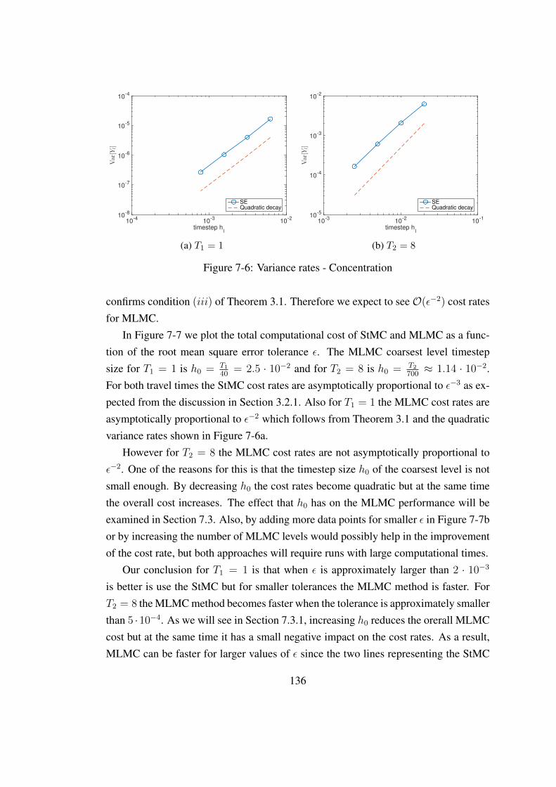
timestep hl

10-4

10-3

10-2

Var[Yl]

10-8

10-7

10-6

10-5

10-4

SEQuadratic decay

(a) T1 = 1

timestep hl

10-3

10-2

10-1

Var[Yl]

10-5

10-4

10-3

10-2

SEQuadratic decay

(b) T2 = 8

Figure 7-6: Variance rates - Concentration

confirms condition (iii) of Theorem 3.1. Therefore we expect to seeO(ε−2) cost ratesfor MLMC.

In Figure 7-7 we plot the total computational cost of StMC and MLMC as a func-tion of the root mean square error tolerance ε. The MLMC coarsest level timestepsize for T1 = 1 is h0 = T1

40= 2.5 · 10−2 and for T2 = 8 is h0 = T2

700≈ 1.14 · 10−2.

For both travel times the StMC cost rates are asymptotically proportional to ε−3 as ex-pected from the discussion in Section 3.2.1. Also for T1 = 1 the MLMC cost rates areasymptotically proportional to ε−2 which follows from Theorem 3.1 and the quadraticvariance rates shown in Figure 7-6a.

However for T2 = 8 the MLMC cost rates are not asymptotically proportional toε−2. One of the reasons for this is that the timestep size h0 of the coarsest level is notsmall enough. By decreasing h0 the cost rates become quadratic but at the same timethe overall cost increases. The effect that h0 has on the MLMC performance will beexamined in Section 7.3. Also, by adding more data points for smaller ε in Figure 7-7bor by increasing the number of MLMC levels would possibly help in the improvementof the cost rate, but both approaches will require runs with large computational times.

Our conclusion for T1 = 1 is that when ε is approximately larger than 2 · 10−3

is better is use the StMC but for smaller tolerances the MLMC method is faster. ForT2 = 8 the MLMC method becomes faster when the tolerance is approximately smallerthan 5 ·10−4. As we will see in Section 7.3.1, increasing h0 reduces the orerall MLMCcost but at the same time it has a small negative impact on the cost rates. As a result,MLMC can be faster for larger values of ε since the two lines representing the StMC

136

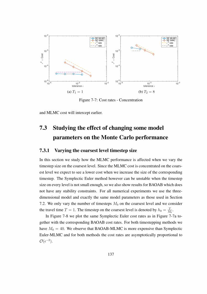
tolerance ǫ

10-4

10-3

10-2

ǫ2 ×

Co

st

10-5

10-4

10-3

10-2

SE MLMC

SE StMC

ǫ-3

rate

ǫ-2

rate

(a) T1 = 1

tolerance ǫ

10-4

10-3

10-2

ǫ2 ×

Co

st

10-5

10-4

10-3

10-2

SE MLMC

SE StMC

ǫ-3

rate

ǫ-2

rate

(b) T2 = 8

Figure 7-7: Cost rates - Concentration

and MLMC cost will intercept earlier.

7.3 Studying the effect of changing some modelparameters on the Monte Carlo performance

7.3.1 Varying the coarsest level timestep size

In this section we study how the MLMC performance is affected when we vary thetimestep size on the coarsest level. Since the MLMC cost is concentrated on the coars-est level we expect to see a lower cost when we increase the size of the correspondingtimestep. The Symplectic Euler method however can be unstable when the timestepsize on every level is not small enough, so we also show results for BAOAB which doesnot have any stability constraints. For all numerical experiments we use the three-dimensional model and exactly the same model parameters as those used in Section7.2. We only vary the number of timesteps M0 on the coarsest level and we considerthe travel time T = 1. The timestep on the coarsest level is denoted by h0 = T

M0.

In Figure 7-8 we plot the same Symplectic Euler cost rates as in Figure 7-7a to-gether with the corresponding BAOAB cost rates. For both timestepping methods wehave M0 = 40. We observe that BAOAB-MLMC is more expensive than SymplecticEuler-MLMC and for both methods the cost rates are asymptotically proportional toO(ε−2).

137

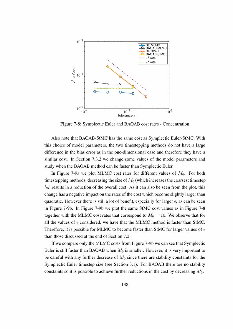
tolerance ǫ

10-4

10-3

10-2

ǫ2 ×

Cost

10-5

10-4

10-3

SE MLMC

BAOAB MLMC

SE StMC

BAOAB StMC

ǫ-3

rate

ǫ-2

rate

Figure 7-8: Symplectic Euler and BAOAB cost rates - Concentration

Also note that BAOAB-StMC has the same cost as Symplectic Euler-StMC. Withthis choice of model parameters, the two timestepping methods do not have a largedifference in the bias error as in the one-dimensional case and therefore they have asimilar cost. In Section 7.3.2 we change some values of the model parameters andstudy when the BAOAB method can be faster than Symplectic Euler.

In Figure 7-9a we plot MLMC cost rates for different values of M0. For bothtimestepping methods, decreasing the size ofM0 (which increases the coarsest timesteph0) results in a reduction of the overall cost. As it can also be seen from the plot, thischange has a negative impact on the rates of the cost which become slightly larger thanquadratic. However there is still a lot of benefit, especially for larger ε, as can be seenin Figure 7-9b. In Figure 7-9b we plot the same StMC cost values as in Figure 7-8together with the MLMC cost rates that correspond to M0 = 10. We observe that forall the values of ε considered, we have that the MLMC method is faster than StMC.Therefore, it is possible for MLMC to become faster than StMC for larger values of εthan those discussed at the end of Section 7.2.

If we compare only the MLMC costs from Figure 7-9b we can see that SymplecticEuler is still faster than BAOAB when M0 is smaller. However, it is very important tobe careful with any further decrease of M0 since there are stability constaints for theSymplectic Euler timestep size (see Section 3.1). For BAOAB there are no stabilityconstaints so it is possible to achieve further reductions in the cost by decreasing M0.

138

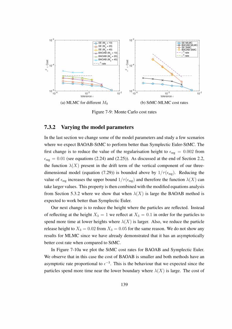
tolerance ǫ10

-410

-310

-2

ǫ2 ×

Co

st

10-5

10-4

10-3

SE (M0 = 10)

SE (M0 = 20)

SE (M0 = 40)

BAOAB (M0 = 10)

BAOAB (M0 = 20)

BAOAB (M0 = 40)

ǫ-3

rate

(a) MLMC for different M0

tolerance ǫ

10-4

10-3

10-2

ǫ2 ×

Co

st

10-5

10-4

10-3

SE MLMC

BAOAB MLMC

SE StMC

BAOAB StMC

ǫ-3

rate

ǫ-2

rate

(b) StMC-MLMC cost rates

Figure 7-9: Monte Carlo cost rates

7.3.2 Varying the model parameters

In the last section we change some of the model parameters and study a few scenarioswhere we expect BAOAB-StMC to perform better than Symplectic Euler-StMC. Thefirst change is to reduce the value of the regularisation height to εreg = 0.002 fromεreg = 0.01 (see equations (2.24) and (2.25)). As discussed at the end of Section 2.2,the function λ(X) present in the drift term of the vertical component of our three-dimensional model (equation (7.29)) is bounded above by 1/τ(εreg). Reducing thevalue of εreg increases the upper bound 1/τ(εreg) and therefore the function λ(X) cantake larger values. This property is then combined with the modified equations analysisfrom Section 5.3.2 where we show that when λ(X) is large the BAOAB method isexpected to work better than Symplectic Euler.

Our next change is to reduce the height where the particles are reflected. Insteadof reflecting at the height X3 = 1 we reflect at X3 = 0.1 in order for the particles tospend more time at lower heights where λ(X) is larger. Also, we reduce the particlerelease height to X3 = 0.02 from X3 = 0.05 for the same reason. We do not show anyresults for MLMC since we have already demonstrated that it has an asymptoticallybetter cost rate when compared to StMC.

In Figure 7-10a we plot the StMC cost rates for BAOAB and Symplectic Euler.We observe that in this case the cost of BAOAB is smaller and both methods have anasymptotic rate proportional to ε−3. This is the behaviour that we expected since theparticles spend more time near the lower boundary where λ(X) is large. The cost of

139

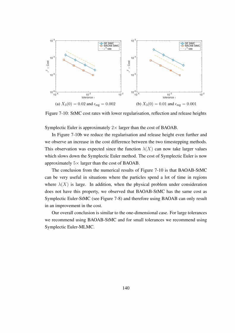
tolerance ǫ

10-4

10-3

10-2

ǫ2 ×

Co

st

10-6

10-5

10-4

10-3

SE StMC

BAOAB StMC

ǫ-3

rate

(a) X3(0) = 0.02 and εreg = 0.002

tolerance ǫ

10-4

10-3

10-2

ǫ2 ×

Co

st

10-6

10-5

10-4

10-3

SE StMC

BAOAB StMC

ǫ-3

rate

(b) X3(0) = 0.01 and εreg = 0.001

Figure 7-10: StMC cost rates with lower regularisation, reflection and release heights

Symplectic Euler is approximately 2× larger than the cost of BAOAB.In Figure 7-10b we reduce the regularisation and release height even further and

we observe an increase in the cost difference between the two timestepping methods.This observation was expected since the function λ(X) can now take larger valueswhich slows down the Symplectic Euler method. The cost of Symplectic Euler is nowapproximately 5× larger than the cost of BAOAB.

The conclusion from the numerical results of Figure 7-10 is that BAOAB-StMCcan be very useful in situations where the particles spend a lot of time in regionswhere λ(X) is large. In addition, when the physical problem under considerationdoes not have this property, we observed that BAOAB-StMC has the same cost asSymplectic Euler-StMC (see Figure 7-8) and therefore using BAOAB can only resultin an improvement in the cost.

Our overall conclusion is similar to the one-dimensional case. For large toleranceswe recommend using BAOAB-StMC and for small tolerances we recommend usingSymplectic Euler-MLMC.

140

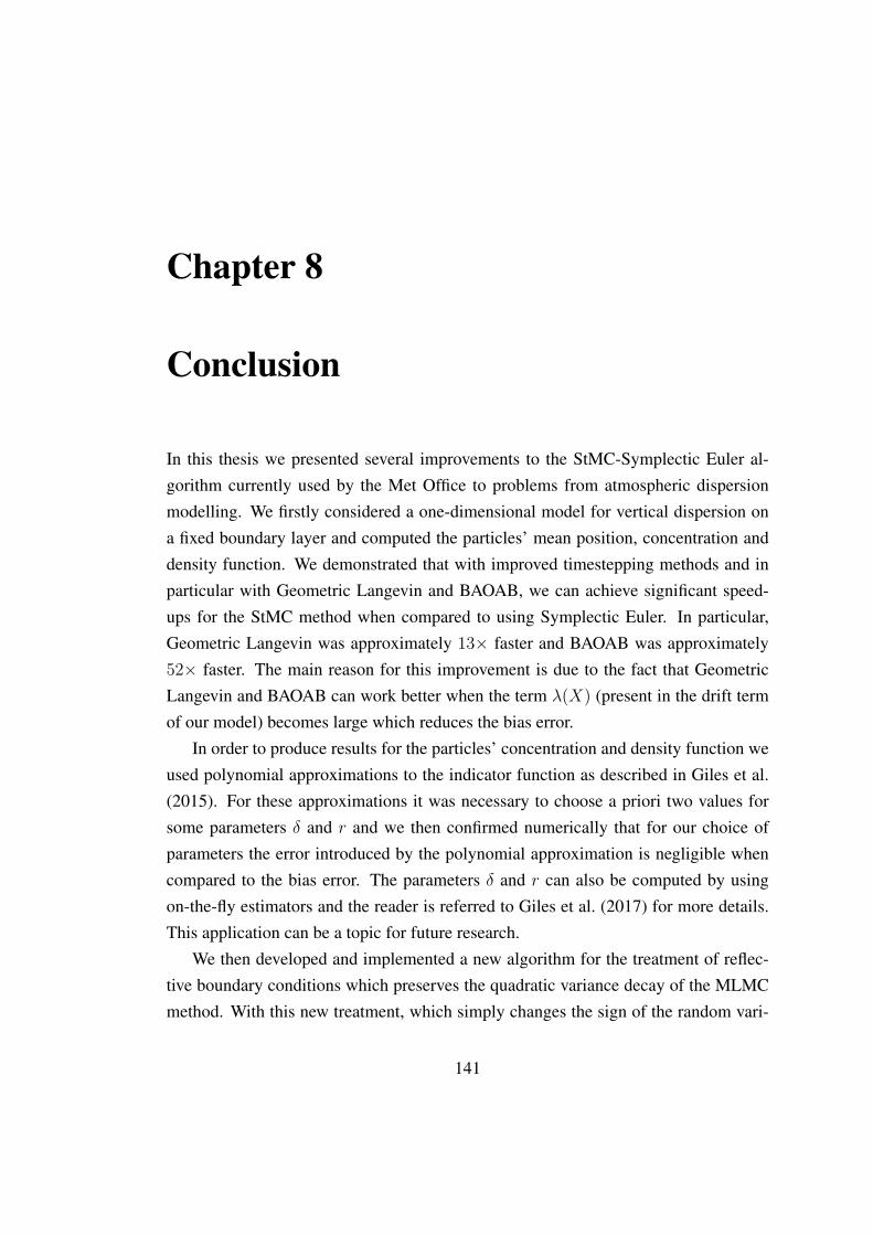
Chapter 8

Conclusion

In this thesis we presented several improvements to the StMC-Symplectic Euler al-gorithm currently used by the Met Office to problems from atmospheric dispersionmodelling. We firstly considered a one-dimensional model for vertical dispersion ona fixed boundary layer and computed the particles’ mean position, concentration anddensity function. We demonstrated that with improved timestepping methods and inparticular with Geometric Langevin and BAOAB, we can achieve significant speed-ups for the StMC method when compared to using Symplectic Euler. In particular,Geometric Langevin was approximately 13× faster and BAOAB was approximately52× faster. The main reason for this improvement is due to the fact that GeometricLangevin and BAOAB can work better when the term λ(X) (present in the drift termof our model) becomes large which reduces the bias error.

In order to produce results for the particles’ concentration and density function weused polynomial approximations to the indicator function as described in Giles et al.(2015). For these approximations it was necessary to choose a priori two values forsome parameters δ and r and we then confirmed numerically that for our choice ofparameters the error introduced by the polynomial approximation is negligible whencompared to the bias error. The parameters δ and r can also be computed by usingon-the-fly estimators and the reader is referred to Giles et al. (2017) for more details.This application can be a topic for future research.

We then developed and implemented a new algorithm for the treatment of reflec-tive boundary conditions which preserves the quadratic variance decay of the MLMCmethod. With this new treatment, which simply changes the sign of the random vari-

141

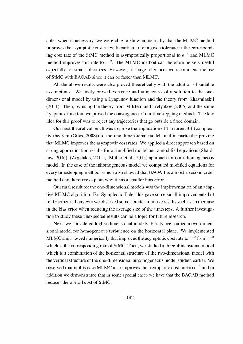
ables when is necessary, we were able to show numerically that the MLMC methodimproves the asymptotic cost rates. In particular for a given tolerance ε the correspond-ing cost rate of the StMC method is asymptotically proportional to ε−3 and MLMCmethod improves this rate to ε−2. The MLMC method can therefore be very usefulespecially for small tolerances. However, for large tolerances we recommend the useof StMC with BAOAB since it can be faster than MLMC.

All the above results were also proved theoretically with the addition of suitableassumptions. We firstly proved existence and uniqueness of a solution to the one-dimensional model by using a Lyapunov function and the theory from Khasminskii(2011). Then, by using the theory from Milstein and Tretyakov (2005) and the sameLyapunov function, we proved the convergence of our timestepping methods. The keyidea for this proof was to reject any trajectories that go outside a fixed domain.

Our next theoretical result was to prove the application of Threorem 3.1 (complex-ity theorem (Giles, 2008)) to the one-dimensional models and in particular provingthat MLMC improves the asymptotic cost rates. We applied a direct approach based onstrong approximation results for a simplified model and a modified equations (Shard-low, 2006), (Zygalakis, 2011), (Muller et al., 2015) approach for our inhomogeneousmodel. In the case of the inhomogeneous model we computed modified equations forevery timestepping method, which also showed that BAOAB is almost a second ordermethod and therefore explain why it has a smaller bias error.

Our final result for the one-dimensional models was the implementation of an adap-tive MLMC algorithm. For Symplectic Euler this gave some small improvements butfor Geometric Langevin we observed some counter-intuitive results such as an increasein the bias error when reducing the average size of the timesteps. A further investiga-tion to study these unexpected results can be a topic for future research.

Next, we considered higher dimensional models. Firstly, we studied a two-dimen-sional model for homogeneous turbulence on the horizontal plane. We implementedMLMC and showed numerically that improves the asymptotic cost rate to ε−2 from ε−3

which is the corresponding rate of StMC. Then, we studied a three-dimensional modelwhich is a combination of the horizontal structure of the two-dimensional model withthe vertical structure of the one-dimensional inhomogeneous model studied earlier. Weobserved that in this case MLMC also improves the asymptotic cost rate to ε−2 and inaddition we demonstrated that in some special cases we have that the BAOAB methodreduces the overall cost of StMC.

142

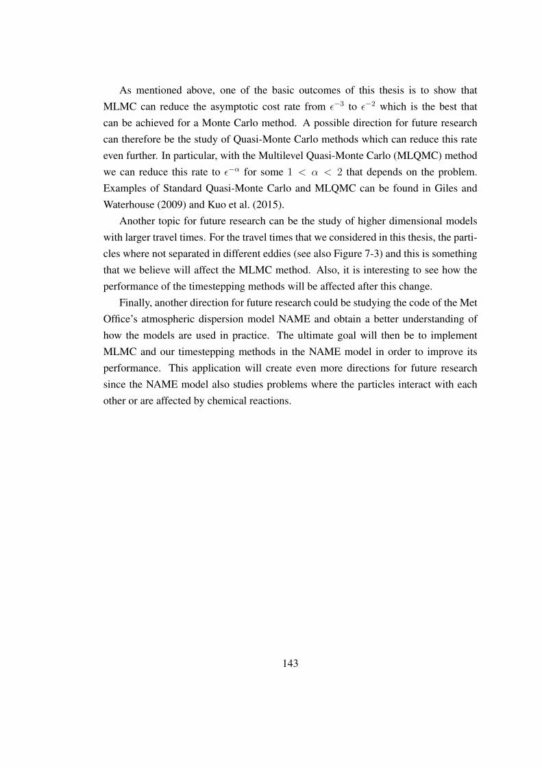
As mentioned above, one of the basic outcomes of this thesis is to show thatMLMC can reduce the asymptotic cost rate from ε−3 to ε−2 which is the best thatcan be achieved for a Monte Carlo method. A possible direction for future researchcan therefore be the study of Quasi-Monte Carlo methods which can reduce this rateeven further. In particular, with the Multilevel Quasi-Monte Carlo (MLQMC) methodwe can reduce this rate to ε−α for some 1 < α < 2 that depends on the problem.Examples of Standard Quasi-Monte Carlo and MLQMC can be found in Giles andWaterhouse (2009) and Kuo et al. (2015).

Another topic for future research can be the study of higher dimensional modelswith larger travel times. For the travel times that we considered in this thesis, the parti-cles where not separated in different eddies (see also Figure 7-3) and this is somethingthat we believe will affect the MLMC method. Also, it is interesting to see how theperformance of the timestepping methods will be affected after this change.

Finally, another direction for future research could be studying the code of the MetOffice’s atmospheric dispersion model NAME and obtain a better understanding ofhow the models are used in practice. The ultimate goal will then be to implementMLMC and our timestepping methods in the NAME model in order to improve itsperformance. This application will create even more directions for future researchsince the NAME model also studies problems where the particles interact with eachother or are affected by chemical reactions.

143

Bibliography

Bernardo, M., Budd, C., Champneys, A. R., and Kowalczyk, P. (2008). Piecewise-

smooth Dynamical Systems: Theory and Applications, volume 163. Springer Sci-ence & Business Media.

Bou-Rabee, N. and Owhadi, H. (2010). Long-run accuracy of variational integratorsin the stochastic context. SIAM Journal on Numerical Analysis, 48(1):278–297.

Cliffe, K., Giles, M. B., Scheichl, R., and Teckentrup, A. L. (2011). Multilevel MonteCarlo methods and applications to elliptic PDEs with random coefficients. Comput-

ing and Visualization in Science, 14(1):3–15.

Cook, S. (2013). Multi Level Monte Carlo Methods for Atmospheric Dispersion Mod-elling. MPhil, University of Bath.

Dacre, H. F., Grant, A. L., Hogan, R. J., Belcher, S. E., Thomson, D., Devenish, B.,Marenco, F., Hort, M., Haywood, J. M., Ansmann, A., Mattis, I., and Clarisse, L.(2011). Evaluating the structure and magnitude of the ash plume during the ini-tial phase of the 2010 Eyjafjallajokull eruption using lidar observations and NAMEsimulations. Journal of Geophysical Research: Atmospheres, 116(D20).

Fung, J. C. H. and Vassilicos, J. C. (1998). Two-particle dispersion in turbulentlikeflows. Physical Review E, 57(2):1677.

George, W. K. (2009). Lectures in Turbulence for the 21st Century. Chalmers Univer-

sity of Technology.

Giles, M. and Szpruch, L. (2012). Multilevel Monte Carlo methods for applications infinance. arXiv preprint arXiv:1212.1377.

144

Giles, M. B. (2008). Multilevel Monte Carlo Path Simulation. OPERATIONS RE-

SEARCH, 56(3):607–617.

Giles, M. B., Lester, C., and Whittle, J. (2016). Non-nested adaptive timesteps in mul-tilevel monte carlo computations. In Monte Carlo and Quasi-Monte Carlo Methods,pages 303–314. Springer.

Giles, M. B., Nagapetyan, T., and Ritter, K. (2015). Multilevel Monte Carlo Approxi-mation of Distribution Functions and Densities. SIAM/ASA Journal on Uncertainty

Quantification, 3(1):267–295.

Giles, M. B., Nagapetyan, T., and Ritter, K. (2017). Adaptive multilevel monte carloapproximation of distribution functions. arXiv preprint arXiv:1706.06869.

Giles, M. B. and Waterhouse, B. J. (2009). Multilevel quasi-Monte Carlo path simula-tion. Advanced Financial Modelling, Radon Series on Computational and Applied

Mathematics, pages 165–181.

Glasserman, P. (2003). Monte Carlo Methods in Financial Engineering, volume 53.Springer Science & Business Media.

Graham, I. G., Scheichl, R., and Ullmann, E. (2015). Mixed Finite Element Analysisof Lognormal Diffusion and Multilevel Monte Carlo Methods. Stochastic Partial

Differential Equations: Analysis and Computations, pages 1–35.

Hairer, E., Lubich, C., and Wanner, G. (2006). Geometric numerical integration:

structure-preserving algorithms for ordinary differential equations, volume 31.Springer Science & Business Media.

Heinrich, S. (2001). Multilevel Monte Carlo Methods. In Margenov, S., Wasniewski,J., and Yalamov, P., editors, Large-Scale Scientific Computing, volume 2179 of Lec-

ture Notes in Computer Science, pages 58–67. Springer Berlin Heidelberg.

Higham, D. J., Mao, X., and Stuart, A. M. (2002). Strong convergence of euler-typemethods for nonlinear stochastic differential equations. SIAM Journal on Numerical

Analysis, 40(3):1041–1063.

145

Hoel, H., Schwerin, E., Szepessy, A., and Tempone, R. (2012). Numerical Analysis of

Multiscale Computations: Proceedings of a Winter Workshop at the Banff Interna-

tional Research Station 2009, chapter Adaptive Multilevel Monte Carlo Simulation,pages 217–234. Springer Berlin Heidelberg.

Hoel, H., Von Schwerin, E., Szepessy, A., and Tempone, R. (2014). Implementationand analysis of an adaptive multilevel monte carlo algorithm. Monte Carlo Methods

and Applications, 20(1):1–41.

Holton, J. (2004). An introduction to dynamic meteorology. Elsevier Academic Press.

Jones, A. (2004). Atmospheric dispersion modelling at the Met Office. Weather,59:311–316.

Jones, A., Thomson, D., Hort, M., and Devenish, B. (2007). The U.K. Met Office’sNext-Generation Atmospheric Dispersion Model, NAME III. Air Pollution Model-

ing and Its Application XVII, pages 580–589.

Karatzas, I. and Shreve, S. (2012). Brownian Motion and Stochastic Calculus, volume113. Springer Science & Business Media.

Katsiolides, G., Mller, E. H., Scheichl, R., Shardlow, T., Giles, M. B., and Thomson,D. J. (2018). Multilevel monte carlo and improved timestepping methods in atmo-spheric dispersion modelling. Journal of Computational Physics, 354(SupplementC):320 – 343.

Khasminskii, R. (2011). Stochastic Stability of Differential Equations, volume 66.Springer Science & Business Media.

Kloeden, P. and Platen, E. (2011). Numerical Solution of Stochastic Differential Equa-

tions. Stochastic Modelling and Applied Probability. Springer Berlin Heidelberg.

Kuo, F. Y., Scheichl, R., Schwab, C., Sloan, I. H., and Ullmann, E. (2015). Multi-level quasi-Monte Carlo methods for lognormal diffusion problems. arXiv preprint

arXiv:1507.01090.

Leadbetter, S. J., Hort, M. C., Jones, A. R., Webster, H. N., and Draxler, R. R. (2015).Sensitivity of the modelled deposition of Caesium-137 from the Fukushima Dai-ichi nuclear power plant to the wet deposition parameterisation in NAME. Journal

of environmental radioactivity, 139:200–211.

146

Leimkuhler, B. and Matthews, C. (2015). Molecular Dynamics: with deterministic

and stochastic numerical methods, volume 39. Springer.

Leimkuhler, B. and Reich, S. (2004). Simulating hamiltonian dynamics, volume 14.Cambridge university press.

Lemieux, C. (2009). Monte Carlo and Quasi-Monte Carlo Sampling. Springer Science& Business Media.

Lord, G. J., Powell, C. E., and Shardlow, T. (2014). An introduction to computational

stochastic PDEs. Number 50. Cambridge University Press.

Metropolis, N. and Ulam, S. (1949). The Monte Carlo Method. Journal of the Ameri-

can Statistical Association, 44(247):335–341.

Milstein, G. and Tretyakov, M. V. (2005). Numerical integration of stochastic differ-ential equations with nonglobally lipschitz coefficients. SIAM journal on numerical

analysis, 43(3):1139–1154.

Mueller, E. H., Katsiolides, G., and Shardlow, T. (2017). MLMCLangevin code.

Muller, E. H., Scheichl, R., and Shardlow, T. (2015). Improving multilevel MonteCarlo for stochastic differential equations with application to the Langevin equation.Proceedings of the Royal Society A, 471(2176).

Nastrom, G. and Gage, K. S. (1985). A climatology of atmospheric wavenumberspectra of wind and temperature observed by commercial aircraft. Journal of the

atmospheric sciences, 42(9):950–960.

Øksendal, B. (2003). Stochastic Differential Equations: An Introduction with Appli-

cations. Springer Berlin Heidelberg.

Ramli, H. M. and Esler, J. G. (2016). Quantitative evaluation of numerical integrationschemes for lagrangian particle dispersion models. Geoscientific Model Develop-

ment, 9(7):2441–2457.

Rodean, H. C. (1996). Stochastic Lagrangian Models of Turbulent Diffusion. Ameri-can Meteorological Society.

147

Shardlow, T. (2006). Modified equations for stochastic differential equations. BIT

Numerical Mathematics, 46(1):111–125.

Smith, F. and Clark, M. J. (1989). The transport and deposition of airborne debrisfrom the Chernobyl nuclear power plant accident with special emphasis on the con-sequences to the United Kingdom. Technical report, Meteorological Office.

Taylor, G. I. (1921). Diffusion by continuous movements. Proc London Math Soc A,20:l96–2ll.

Thomson, D. and Devenish, B. (2005). Particle pair separation in kinematic simula-tions. Journal of Fluid Mechanics, 526:277–302.

Thomson, D. J. (1987). Criteria for the selection of stochastic models of particletrajectories in turbulent flows. Journal of Fluid Mechanics, 180:529–556.

Wang, F.-Y. and Zhang, X. (2016). Degenerate SDE with Holder-Dini Drift and Non-Lipschitz Noise Coefficient. SIAM Journal on Mathematical Analysis, 48(3):2189–2226.

Watanabe, S. and Ikeda, N. (1981). Stochastic Differential Equations and Diffusion

Processes, volume 24. Elsevier.

Webster, H., Thomson, D., Johnson, B., Heard, I., Turnbull, K., Marenco, F., Kris-tiansen, N., Dorsey, J., Minikin, A., Weinzierl, B., Schumann, U., Sparks, R.,Loughlin, S., Hort, M., Leadbetter, S., Devenish, B., Manning, A., Witham, C.,Haywood, J., and Golding, B. (2012). Operational prediction of ash concentrationsin the distal volcanic cloud from the 2010 Eyjafjallajokull eruption. Journal of Geo-

physical Research: Atmospheres, 117(D20).

Webster, H., Thomson, D., and Morrison, N. (2003). New turbulence profiles forNAME. Met Office Turbulence and Diffusion note 288.

Wilson, J., Yee, E., Ek, N., and d’Amours, R. (2009). Lagrangian simulation of windtransport in the urban environment. Quarterly Journal of the Royal Meteorological

Society, 135(643):1586–1602.

Zygalakis, K. C. (2011). On the existence and the applications of modified equa-tions for stochastic differential equations. SIAM Journal on Scientific Computing,33(1):102–130.

148

Appendix A

A.1 Verifying equation (2.17)

The simplified model is given by

dU(t) = −U(t)

τdt+

√2σ2

U

τdW (t). (A.1)

This is an Ornstein-Uhlenbeck process so in order to find the solution we follow thestandard technique by considering the random variable Y (t) = e

1τtU(t).

Applying Ito’s formula to Y (t) gives

dY (t) =

√2σ2

U

τe

1τtdW (t). (A.2)

Since τ and σU are constants we assume for simplicity that the system is at equilibriumby setting the start time equal to minus infinity. Integrating equation (A.2) gives

Y (t) =

√2σ2

U

τ

∫ t

−∞e

1τsdW (s), (A.3)

which implies

U(t) =

√2σ2

U

τe−

1τt

∫ t

−∞e

1τsdW (s). (A.4)

149

Therefore, U(t) is Gaussian with mean zero and variance

V ar(U(t)) =2σ2

U

τe−

2τtV ar

(∫ t

−∞e

1τsdW (s)

)=

2σ2U

τe−

2τtE(∫ t

−∞e

1τsdW (s)

)2

=2σ2

U

τe−

2τt

∫ t

−∞e

2τsds (Ito isometry)

= σ2U .

Then,

〈U(t)U(t0)〉 =2σ2

U

τe−

1τte−

1τt0〈∫ t

−∞e

1τsdW (s)

∫ t0

−∞e

1τsdW (s)〉

=2σ2

U

τe−

1τte−

1τt0

[〈∫ t0

−∞e

1τsdW (s)

∫ t0

−∞e

1τsdW (s)〉

+ 〈∫ t

t0

e1τsdW (s)

∫ t0

−∞e

1τsdW (s)〉

]=

2σ2U

τe−

1τte−

1τt0

[〈(∫ t0

−∞e

1τsdW (s)

)2

〉

+ 〈∫ t

t0

e1τsdW (s)〉〈

∫ t0

−∞e

1τsdW (s)〉

]by independence

=2σ2

U

τe−

1τte−

1τt0

[E(∫ t0

−∞e

1τsdW (s)

)2]

=2σ2

U

τe−

1τte−

1τt0

(∫ t0

−∞e

2τsds

)= σ2

Ue−(t−t0)/τ .

By definition of R

R(t− t0) =〈U(t)U(t0)〉〈U2(t0)〉

=σ2Ue−(t−t0)/τ

σ2U

= e−(t−t0)/τ ,

150

which is equal to equation (2.17).

A.2 One-dimensional homogeneous model - Exactsolution and particle spread

We now compute the exact solution and an expression of the particle spread for theone-dimensional homogeneous model given by

dU(t) = −λU(t)dt+ σdW (t), (A.5)

dX(t) = U(t)dt, (A.6)

with λ = 1τ

and σ =

√2σ2U

τpositive constants.

A.2.1 Exact solution

For the exact solution we let

Y(t) =

(X(t)

U(t)

), Λ =

(0 1

0 −λ

), Σ =

(0

σ

)(A.7)

so that equations (A.5) and (A.6) can be written as the following Ornstein-Uhlenbeckprocess

dY(t) = ΛY(t)dt+ ΣdW(t). (A.8)

Applying Ito’s formula to Z(t) = e−ΛtY(t) gives

dZ(t) = e−ΛtΣdW(t). (A.9)

Integrating gives

Z(t) = Z(0) +

∫ t

0

e−ΛsΣdW(s), (A.10)

which implies that

Y(t) = eΛtY(0) +

∫ t

0

e−Λ(s−t)ΣdW(s). (A.11)

151

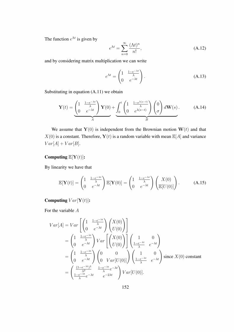
The function eΛt is given by

eΛt =∞∑n=0

(Λt)n

n!, (A.12)

and by considering matrix multiplication we can write

eΛt =

(1 1−e−λt

λ

0 e−λt

). (A.13)

Substituting in equation (A.11) we obtain

Y(t) =

(1 1−e−λt

λ

0 e−λt

)Y(0)︸ ︷︷ ︸

A

+

∫ t

0

(1 1−eλ(s−t)

λ

0 eλ(s−t)

)(0

σ

)dW(s)︸ ︷︷ ︸

B

. (A.14)

We assume that Y(0) is independent from the Brownian motion W(t) and thatX(0) is a constant. Therefore, Y(t) is a random variable with mean E[A] and varianceV ar[A] + V ar[B].

Computing E[Y(t)]:

By linearity we have that

E[Y(t)] =

(1 1−e−λt

λ

0 e−λt

)E[Y(0)] =

(1 1−e−λt

λ

0 e−λt

)(X(0)

E[U(0)]

). (A.15)

Computing V ar[Y(t)]:

For the variable A

V ar[A] = V ar

[(1 1−e−λt

λ

0 e−λt

)(X(0)

U(0)

)]

=

(1 1−e−λt

λ

0 e−λt

)V ar

[(X(0)

U(0)

)](1 0

1−e−λtλ

e−λt

)

=

(1 1−e−λt

λ

0 e−λt

)(0 0

0 V ar[U(0)]

)(1 0

1−e−λtλ

e−λt

)since X(0) constant

=

((1−e−λt)2

λ21−e−λt

λe−λt

1−e−λtλ

e−λt e−2λt

)V ar[U(0)].

152

For the variable B

V ar[B] = V ar

[∫ t

0

(σλ(1− eλ(s−t))

σeλ(s−t)

)dW(s)

]

=

∫ t

0

(σλ(1− eλ(s−t))

σeλ(s−t)

)(σλ(1− eλ(s−t)) σeλ(s−t)

)ds

=

(σ2

2λ3 (2λt− 3 + 4e−λt − e−2λt) σ2

2λ2 (1− 2e−λt + e−2λt)σ2

2λ2 (1− 2e−λt + e−2λt) σ2

2λ(1− e−2λt)

)

By sampling from the distribution of the random variable U(0) and by knowing themean and covariance matrix of the normally distributed random variable B we havethe exact solution of the homogeneous model.

A.2.2 Particle spread

As described in Section 7.1.4 the particle spread is given by the standard deviation ofXt i.e.

√V ar[X(t)]. From Section A.2.1 we have

V ar[X(t)] =(1− e−λt)2

λ2V ar[U(0)] +

σ2

2λ3(2λt− 3 + 4e−λt − e−2λt), (A.16)

and by taking the square root we have an expression for the particle spread with respectto time. Next, we analyse how the short and long time behaviour of the spread isaffected by the choice of U(0) which can be deterministic or random.

Deterministic U(0)

When U(0) is deterministic we have that V ar[U(0)] = 0 which gives

V ar[X(t)] =σ2

2λ3(2λt− 3 + 4e−λt − e−2λt). (A.17)

For the short time behaviour we Taylor expand equation (A.17) to obtain

V ar[X(t)] =σ2

3t3 + higher order terms, (A.18)

153

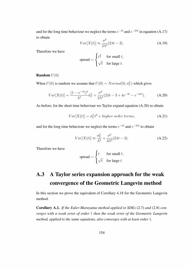
and for the long time behaviour we neglect the terms e−λt and e−2λt in equation (A.17)to obtain

V ar[X(t)] ≈ σ2

2λ3(2λt− 3). (A.19)

Therefore we have

spread ∼

t32 for small t,√t for large t.

Random U(0)

When U(0) is random we assume that U(0) ∼ Normal(0, σ2U) which gives

V ar[X(t)] =(1− e−λt)2

λ2σ2U +

σ2

2λ3(2λt− 3 + 4e−λt − e−2λt). (A.20)

As before, for the short time behaviour we Taylor expand equation (A.20) to obtain

V ar[X(t)] = σ2U t

2 + higher order terms, (A.21)

and for the long time behaviour we neglect the terms e−λt and e−2λt to obtain

V ar[X(t)] ≈ σ2U

λ2+

σ2

2λ3(2λt− 3). (A.22)

Therefore we have

spread ∼

t for small t,√t for large t.

A.3 A Taylor series expansion approach for the weakconvergence of the Geometric Langevin method

In this section we prove the equivalent of Corollary 4.18 for the Geometric Langevinmethod.

Corollary A.1. If the Euler-Maruyama method applied to SDEs (2.7) and (2.8) con-

verges with a weak error of order 1 then the weak error of the Geometric Langevin

method, applied to the same equations, also converges with at least order 1.

154

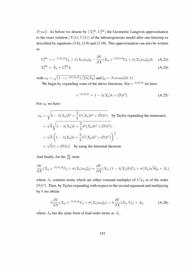
Proof . As before we denote by (XGL1 , UGL

1 ) the Geometric Langevin approximationto the exact solution (X(h), U(h)) of the inhomogeneous model after one timestep asdescribed by equations (3.8), (3.9) and (3.10). This approximation can also be writtenas

UGL1 = e−λ(X0)hU0 + σ(X0)αhξ0 −

∂V

∂X(X0, e

−λ(X0)hU0 + σ(X0)αhξ0)h, (A.23)

XGL1 = X0 + UGL

1 h, (A.24)

with αh =√

(1− e−2λ(X0)h) /2λ(X0) and ξ0 ∼ Normal(0, 1).We begin by expanding some of the above functions. For e−λ(X0)h we have

e−λ(X0)h = 1− λ(X0)h+O(h2). (A.25)

For αh we have

αh =

√h− λ(X0)h2 +

2

3λ2(X0)h3 +O(h4) by Taylor expanding the numerator,

=√h

√1− λ(X0)h+

2

3λ2(X0)h2 +O(h3),

=√h

(1− λ(X0)h+

2

3λ2(X0)h2 +O(h3)

) 12

,

=√h(1 +O(h)) by using the binomial theorem.

And finally, for the ∂V∂X

term

∂V

∂X(X0, e

−λ(X0)hU0 + σ(X0)αhξ0) =∂V

∂X(X0, (1− λ(X0)h)U0 + σ(X0)

√hξ0 + A1),

where A1 contains terms which are either constant multiples of h32 ξ0 or of the order

O(h2). Then, by Taylor expanding with respect to the second argument and multipyingby h we obtain

h∂V

∂X(X0, e

−λ(X0)hU0 + σ(X0)αhξ0) = h∂V

∂X(X0, U0) + A2, (A.26)

where A2 has the same form of lead order terms as A1.

155

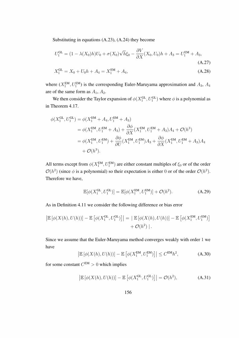
Substituting in equations (A.23), (A.24) they become

UGL1 = (1− λ(X0)h)U0 + σ(X0)

√hξ0 −

∂V

∂X(X0, U0)h+ A3 = UEM

1 + A3,

(A.27)

XGL1 = X0 + U0h+ A4 = XEM

1 + A4, (A.28)

where (XEM1 , UEM

1 ) is the corresponding Euler-Maruyama approximation and A3, A4

are of the same form as A1, A2.We then consider the Taylor expansion of φ(XGL

1 , UGL1 ) where φ is a polynomial as

in Theorem 4.17.

φ(XGL1 , UGL

1 ) = φ(XEM1 + A4, U

EM1 + A3)

= φ(XEM1 , UEM

1 + A3) +∂φ

∂X(XEM

1 , UEM1 + A3)A4 +O(h3)

= φ(XEM1 , UEM

1 ) +∂φ

∂U(XEM

1 , UEM1 )A3 +

∂φ

∂X(XEM

1 , UEM1 + A3)A4

+O(h3).

All terms except from φ(XEM1 , UEM

1 ) are either constant multiples of ξ0 or of the orderO(h2) (since φ is a polynomial) so their expectation is either 0 or of the order O(h2).Therefore we have,

E[φ(XGL1 , UGL

1 )] = E[φ(XEM1 , UEM

1 )] +O(h2). (A.29)

As in Definition 4.11 we consider the following difference or bias error

∣∣E [φ(X(h), U(h))]− E[φ(XGL

1 , UGL1 )]∣∣ = | E [φ(X(h), U(h))]− E

[φ(XEM

1 , UEM1 )]

+O(h2) | .

Since we assume that the Euler-Maruyama method converges weakly with order 1 wehave ∣∣E [φ(X(h), U(h))]− E

[φ(XEM

1 , UEM1 )]∣∣ ≤ CEMh2, (A.30)

for some constant CEM > 0 which implies

∣∣E [φ(X(h), U(h))]− E[φ(XGL

1 , UGL1 )]∣∣ = O(h2), (A.31)

156

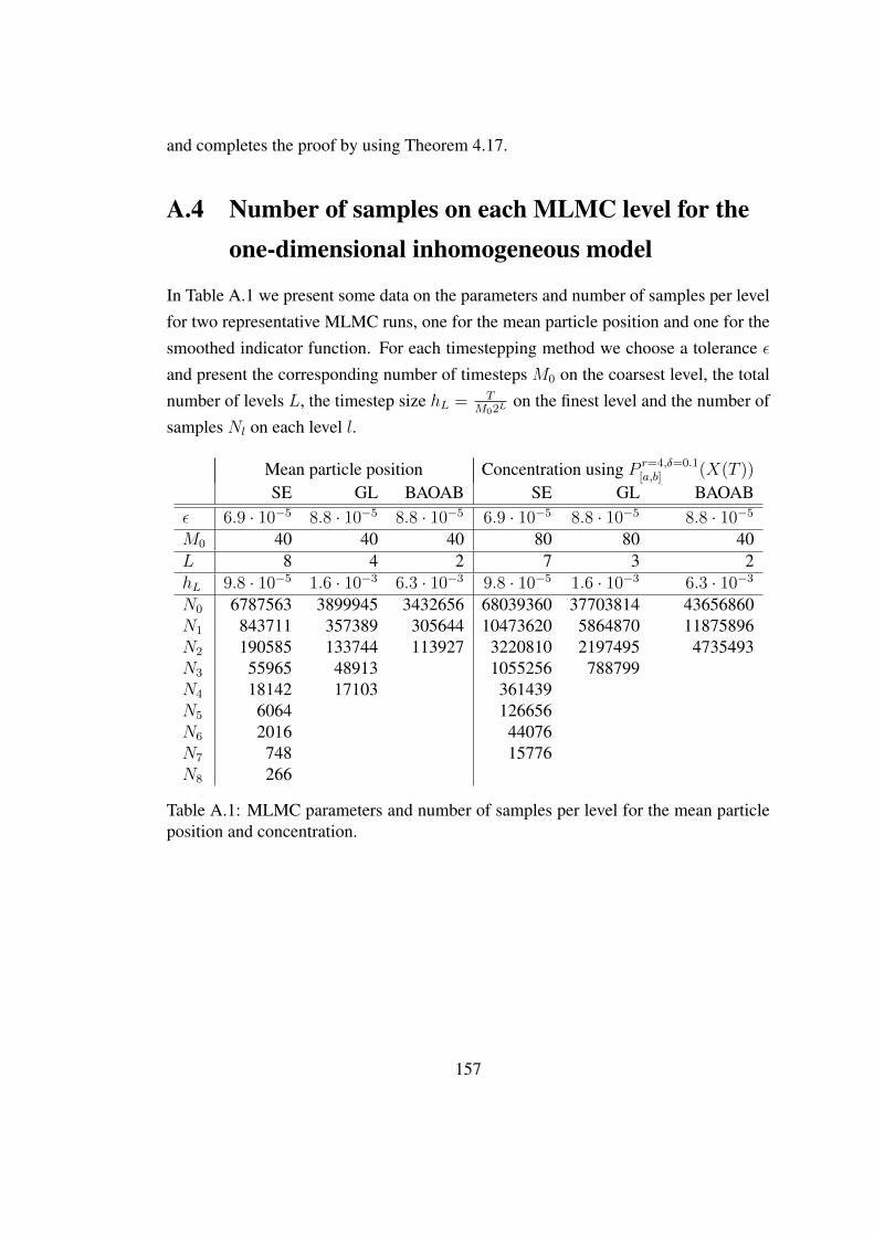
and completes the proof by using Theorem 4.17.

A.4 Number of samples on each MLMC level for theone-dimensional inhomogeneous model

In Table A.1 we present some data on the parameters and number of samples per levelfor two representative MLMC runs, one for the mean particle position and one for thesmoothed indicator function. For each timestepping method we choose a tolerance εand present the corresponding number of timesteps M0 on the coarsest level, the totalnumber of levels L, the timestep size hL = T

M02Lon the finest level and the number of

samples Nl on each level l.

Mean particle position Concentration using P r=4,δ=0.1[a,b] (X(T ))

SE GL BAOAB SE GL BAOABε 6.9 · 10−5 8.8 · 10−5 8.8 · 10−5 6.9 · 10−5 8.8 · 10−5 8.8 · 10−5

M0 40 40 40 80 80 40L 8 4 2 7 3 2hL 9.8 · 10−5 1.6 · 10−3 6.3 · 10−3 9.8 · 10−5 1.6 · 10−3 6.3 · 10−3

N0 6787563 3899945 3432656 68039360 37703814 43656860N1 843711 357389 305644 10473620 5864870 11875896N2 190585 133744 113927 3220810 2197495 4735493N3 55965 48913 1055256 788799N4 18142 17103 361439N5 6064 126656N6 2016 44076N7 748 15776N8 266

Table A.1: MLMC parameters and number of samples per level for the mean particleposition and concentration.

157