MULTILEVEL FAST MULTIPOLE METHODFOR MODELING PERMEABLE STRUCTURES

USING CONFORMAL FINITE ELEMENTS

by

Kubilay Sertel

A dissertation submitted in partial fulfilmentof the requirements for the degree of

Doctor of Philosophy(Electrical Engineering)

in the University of Michigan2003

Doctoral Committee:

Professor John L. Volakis, ChairProfessor Robert KrasnyResearch Scientist Valdis V. LiepaProfessor Thomas B. A. Senior

Copyright c©Kubilay Sertel

All Rights Reserved2003

ABSTRACT

MULTILEVEL FAST MULTIPOLE METHOD FOR MODELING PERMEABLE

STRUCTURES USING CONFORMAL FINITE ELEMENTS

by

Kubilay Sertel

Chair: John L. Volakis

The analysis of penetrable structures has traditionally been carried out using par-

tial differential equation methods due to the large computation time and memory

requirements of integral equation methods. To reduce this computational bottle-

neck, this thesis focuses on fast integral equation methods for modeling penetrable

geometries with both dielectric and magnetic material properties.

Previous works have employed the multilevel fast multipole method for impen-

etrable targets in the context of flat-triangular geometry approximations. In this

thesis, we integrate the multilevel fast multipole method with surface and volume

integral equation techniques to accurately analyze arbitrarily curved inhomogeneous

targets. It is demonstrated that conformal geometry modeling using curvilinear el-

ements achieve higher accuracy at lower sampling rates. Also, the combined use of

curvilinear elements and the multilevel fast multipole method allows for significantly

faster and more efficient numerical methods.

The proposed method reduces the traditional O(N2) computational cost down

to O(N log N) and thus practical size geometries can be analyzed. Several example

calculations are given in the thesis along with comparisons with partial differential

equation methods.

∇× E(r, t) = − ∂

∂tB(r, t),

∇×H(r, t) = − ∂

∂tD(r, t) + J(r, t),

∇ ·B(r, t) = 0,

∇ ·D(r, t) = ρ(r, t).

Dedicated to my parents and my brother.

ii

ACKNOWLEDGMENTS

During my 5.5 years at the University of Michigan, I had the chance to meet a

lot great people. Among many them, I would like to name a few that have helped

me with their personal and professional support. I feel very happy to have met these

great people and value their friendship a lot. Dr. Michael A. Carr, Dr. Dejan S.

Filipovic, Mr. Rick W. Kindt, Mr. Dimitris Psychodakis, and Mr. Eng-Swee Siah, I

would like to thank all of you guys for making the VCC a great experience.

I would like to thank my committee members, Professor Robert Krasny from

Mathematics Department and Professor Thomas B. A. Senior and Professor Valdis V.

Liepa from Electrical Engineering and Computer Science Department, for reviewing

my work and providing their suggestions.

And finally, I am grateful to my advisor Prof. John L. Volakis for providing all the

help and guidance, both professionally and personally, during my Ph.D. study here

at Ann Arbor. I consider myself very lucky to have met him and his lovely family,

and I am looking forward to continuing to work with in the future.

iii

CONTENTS

DEDICATION . . . . . . . . . . . . . . . . . . . . . . . . . . . . . . . . . . . . . . . . . . . . . . ii

ACKNOWLEDGMENTS . . . . . . . . . . . . . . . . . . . . . . . . . . . . . . . . . . . . . . iii

LIST OF FIGURES . . . . . . . . . . . . . . . . . . . . . . . . . . . . . . . . . . . . . . . . . . vi

LIST OF TABLES . . . . . . . . . . . . . . . . . . . . . . . . . . . . . . . . . . . . . . . . . . . xi

LIST OF APPENDICES . . . . . . . . . . . . . . . . . . . . . . . . . . . . . . . . . . . . . . . xii

CHAPTER

1 Introduction . . . . . . . . . . . . . . . . . . . . . . . . . . . . . . . . . . . . . . . . . 1

2 Surface Integral Equations . . . . . . . . . . . . . . . . . . . . . . . . . . . . . . 8

2.1 Surface Integral Equations for PEC Structures . . . . . . . . . . . . . . 8

2.2 Geometry Modelling and Basis Functions . . . . . . . . . . . . . . . . . 10

2.3 MoM Procedure for EFIE . . . . . . . . . . . . . . . . . . . . . . . . . . . . 13

2.4 Examples and Validations . . . . . . . . . . . . . . . . . . . . . . . . . . . . 21

3 Fast Multipole Method and Its Multilevel Implementation . . . . 30

3.1 Fast Multipole Method . . . . . . . . . . . . . . . . . . . . . . . . . . . . . . 32

3.2 Multilevel Fast Multipole Method . . . . . . . . . . . . . . . . . . . . . . . 43

3.3 Multilevel Fast Multipole Method Formulation . . . . . . . . . . . . . . 45

3.4 Examples and Validations . . . . . . . . . . . . . . . . . . . . . . . . . . . . 51

4 Hybrid Finite Element-Boundary Integral Method for Volu-

metric Problems . . . . . . . . . . . . . . . . . . . . . . . . . . . . . . . . . . . . . . 59

4.1 FE-BI Formulation . . . . . . . . . . . . . . . . . . . . . . . . . . . . . . . . . 60

4.2 Geometry Modeling and Basis Functions . . . . . . . . . . . . . . . . . . 64

iv

4.3 MLFMM for FE-BI . . . . . . . . . . . . . . . . . . . . . . . . . . . . . . . . . 69

4.4 FE-BI-MLFMM Validation . . . . . . . . . . . . . . . . . . . . . . . . . . . 71

5 Volume Integral Equations . . . . . . . . . . . . . . . . . . . . . . . . . . . . . . 75

5.1 Volume Integral Equation: General Formulation . . . . . . . . . . . . . 76

5.2 MoM formulation of the VIE for dielectrics . . . . . . . . . . . . . . . . 79

5.2.1 Zeroth-Order Volumetric Basis Functions . . . . . . . . . . . 80

5.2.2 First-Order Volumetric Basis Functions . . . . . . . . . . . . 81

5.2.3 Second-Order Volumetric Basis Functions . . . . . . . . . . 83

5.2.4 Validations for Dielectric Structures . . . . . . . . . . . . . . . 83

5.3 A Comparison of VIE and FE-BI Methods . . . . . . . . . . . . . . . . 86

5.4 MLFMM for Volume Integral Equations . . . . . . . . . . . . . . . . . . 88

5.5 MoM formulation of VIE for Magnetically Permeable Structures . 95

6 Conclusions . . . . . . . . . . . . . . . . . . . . . . . . . . . . . . . . . . . . . . . . . . 102

APPENDICES . . . . . . . . . . . . . . . . . . . . . . . . . . . . . . . . . . . . . . . . . . . . . . 106

BIBLIOGRAPHY . . . . . . . . . . . . . . . . . . . . . . . . . . . . . . . . . . . . . . . . . . . . 129

v

LIST OF FIGURES

Figure

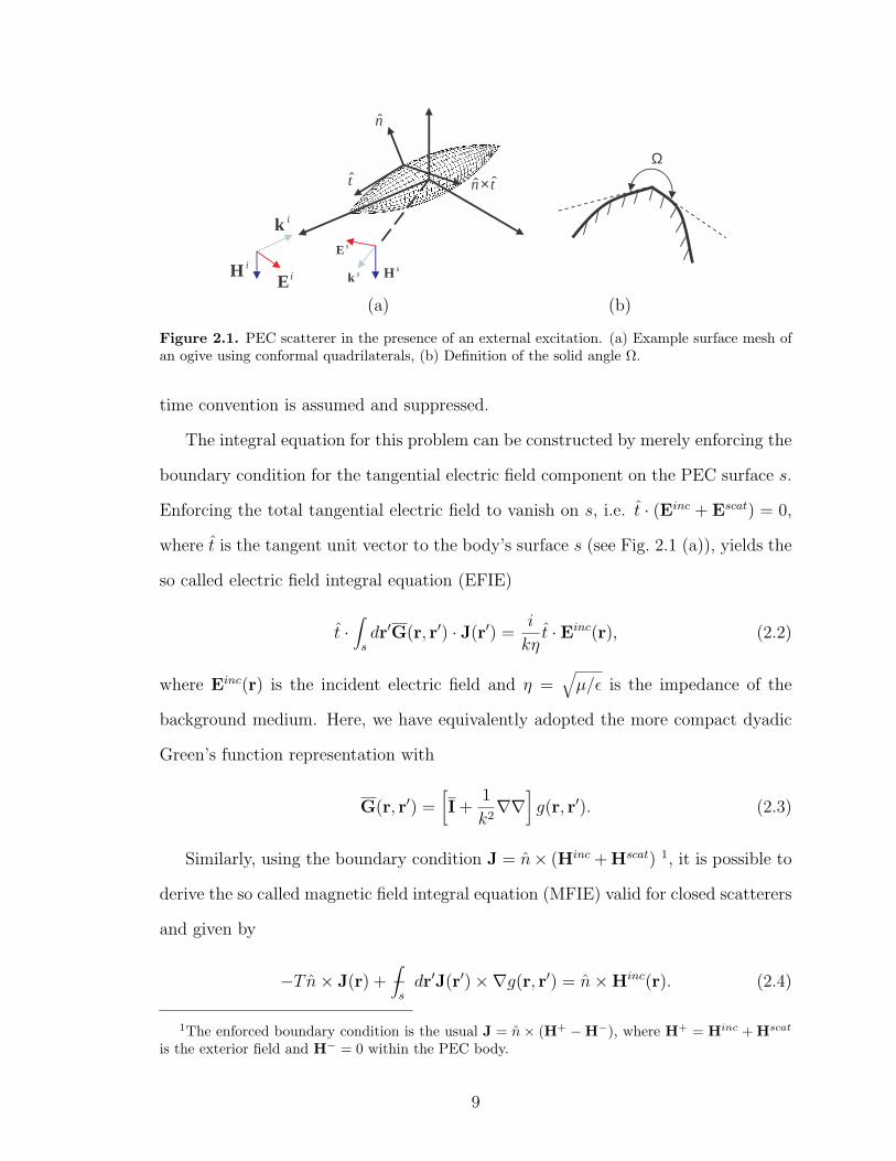
2.1 PEC scatterer in the presence of an external excitation. (a) Example

surface mesh of an ogive using conformal quadrilaterals, (b) Definition

of the solid angle Ω. . . . . . . . . . . . . . . . . . . . . . . . . . . . . . . . . . . . . 9

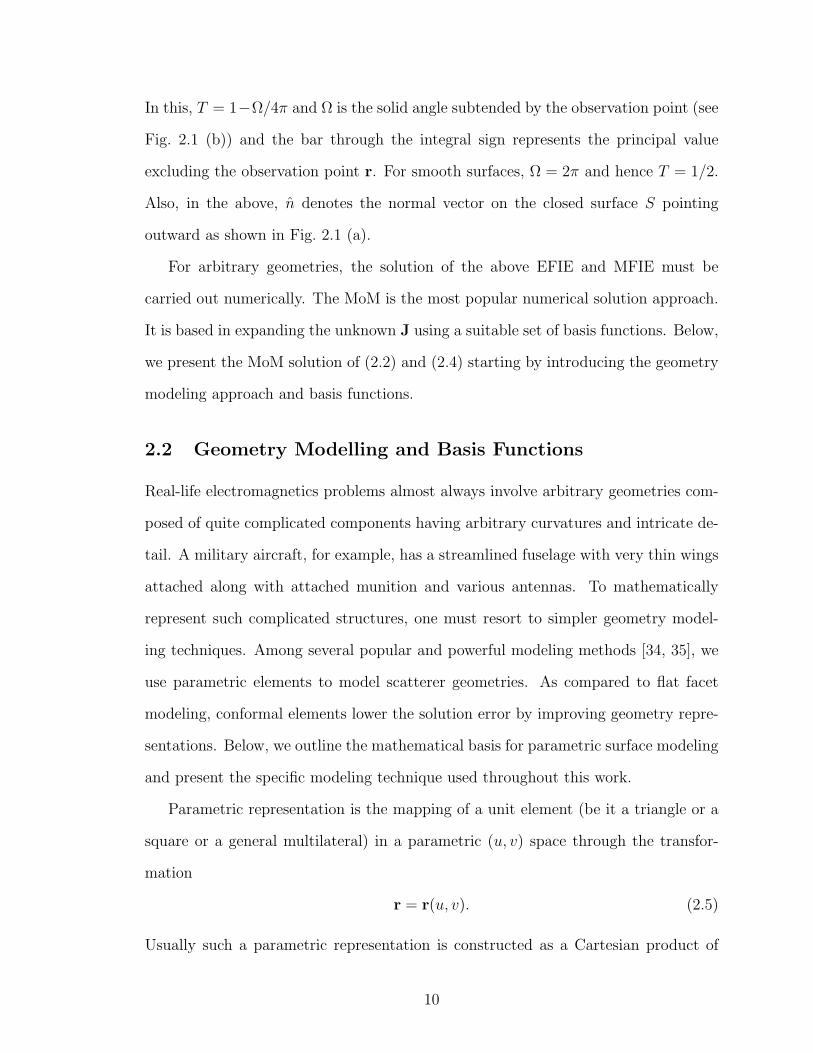
2.2 Examples of parametric mappings. . . . . . . . . . . . . . . . . . . . . . . . . . . 11

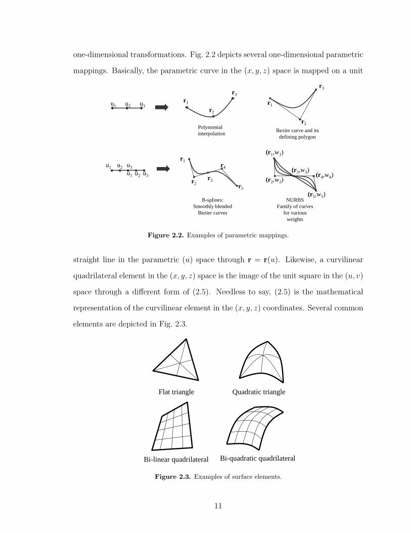
2.3 Examples of surface elements. . . . . . . . . . . . . . . . . . . . . . . . . . . . . . 11

2.4 Curvilinear parametric surface element defined by 9 points. . . . . . . . . 12

2.5 Generic VFY218 aircraft modelled by quadrilateral patches. . . . . . . . . 13

2.6 Constructing basis functions: (a) Two patches forming the support of

basis function associated with the common edge, (b) Quiver plot of

the conformal basis (length of arrows is associated with the amplitude

of the basis function). . . . . . . . . . . . . . . . . . . . . . . . . . . . . . . . . . . . 16

2.7 Illustration for the computation of the element matrices. . . . . . . . . . . 18

2.8 Application of the divergence theorem on the testing function. . . . . . . 19

2.9 Several orders of Gaussian quadrature points for −1 < u < 1 and

−1 < v < 1. . . . . . . . . . . . . . . . . . . . . . . . . . . . . . . . . . . . . . . . . . . 20

2.10 Test geometries: (a) Sphere, (b) Cube, (c) Cylinder, (d) Open-ended

cylinder, (e) Pyramid, (f) Ogive. . . . . . . . . . . . . . . . . . . . . . . . . . . . 21

2.11 Two different meshing methods for a circle: (a) Isoparametric mesh,

(b) Paver mesh. . . . . . . . . . . . . . . . . . . . . . . . . . . . . . . . . . . . . . . . 22

2.12 Bistatic scattering results for the sphere using the EFIE. . . . . . . . . . . 22

2.13 Bistatic scattering results for the sphere using the CFIE with (α = 0.5). 24

vi

2.14 Bistatic scattering results for the sphere using the MFIE . . . . . . . . . . 25

2.15 Bistatic scattering results for the cube using the EFIE and the CFIE

(α = 0.5). . . . . . . . . . . . . . . . . . . . . . . . . . . . . . . . . . . . . . . . . . . . 25

2.16 Bistatic scattering results for the cylinder using the EFIE and the

CFIE (α = 0.5). . . . . . . . . . . . . . . . . . . . . . . . . . . . . . . . . . . . . . . . 26

2.17 Bistatic scattering results for the open cylinder. . . . . . . . . . . . . . . . . 26

2.18 Bistatic scattering results for the pyramid using the EFIE and the

CFIE (α = 0.5). . . . . . . . . . . . . . . . . . . . . . . . . . . . . . . . . . . . . . . . 27

2.19 Bistatic scattering results for the ogive using the EFIE and the CFIE

(α = 0.5). . . . . . . . . . . . . . . . . . . . . . . . . . . . . . . . . . . . . . . . . . . . 28

2.20 Induced surface currents on test targets. . . . . . . . . . . . . . . . . . . . . . . 28

3.1 Groups of basis and testing functions. . . . . . . . . . . . . . . . . . . . . . . . 33

3.2 Vector definitions for Gegenbauer’s addition theorem. . . . . . . . . . . . . 33

3.3 Vector definitions for FMM expansion. . . . . . . . . . . . . . . . . . . . . . . . 34

3.4 Illustration of single level interactions between source and testing clus-

ters in FMM . . . . . . . . . . . . . . . . . . . . . . . . . . . . . . . . . . . . . . . . . 38

3.5 3-levels of k-means clustering example. . . . . . . . . . . . . . . . . . . . . . . . 42

3.6 Illustration of the near-zone threshold in FMM. . . . . . . . . . . . . . . . . 43

3.7 Association of basis functions with points in space (the mid-points of

the edges in the surface mesh). . . . . . . . . . . . . . . . . . . . . . . . . . . . . 44

3.8 Zeroth level cube enclosing the geometry. . . . . . . . . . . . . . . . . . . . . . 44

3.9 First, second, and third level grouping example. . . . . . . . . . . . . . . . . 45

3.10 Two level FMM construct for a general multilevel case. . . . . . . . . . . . 45

3.11 Illustration of interpolation matrices in FMM. . . . . . . . . . . . . . . . . . 47

3.12 Illustration of two level interactions between source and testing groups

in FMM. . . . . . . . . . . . . . . . . . . . . . . . . . . . . . . . . . . . . . . . . . . . . 49

3.13 2-dimensional multilevel clustering example. . . . . . . . . . . . . . . . . . . . 50

vii

3.14 Induced surface currents on the sphere due to the Hertzian dipole. . . . 52

3.15 Radiation patterns (linear-scale) of the Hertzian dipole over the sphere,

solid: Mie solution, dashed: MLFMM. . . . . . . . . . . . . . . . . . . . . . . . 52

3.16 Bistatic RCS of a flat plate using 3-level FMM. . . . . . . . . . . . . . . . . . 54

3.17 Complexities of various levels of the FMM. . . . . . . . . . . . . . . . . . . . . 55

3.18 Bistatic RCS of an 8λ diameter PEC sphere using 7, 500 unknowns. . . 56

3.19 Bistatic RCS of an 8λ diameter PEC sphere using 28, 812 unknowns. . 57

3.20 Bistatic RCS of an 16λ diameter PEC sphere using 28, 812 unknowns. . 57

3.21 Bistatic RCS of an 16λ diameter PEC sphere using 110, 190 unknowns. 58

4.1 FE-BI solution domain. . . . . . . . . . . . . . . . . . . . . . . . . . . . . . . . . . 60

4.2 Real space as a mapping of the parametric space. . . . . . . . . . . . . . . . 64

4.3 Quadratic hexahedral finite element. . . . . . . . . . . . . . . . . . . . . . . . . 67

4.4 Local numbering of the edges of the hexahedral element . . . . . . . . . . 68

4.5 MLFMM procedure for the FE-BI system. . . . . . . . . . . . . . . . . . . . . 70

4.6 Bistatic RCS of a dielectric sphere using the FE-BI method. . . . . . . . 72

4.7 Bistatic RCS of a coated sphere using the FE-BI method. . . . . . . . . . 73

4.8 Bistatic RCS of a coated sphere using the MLFMM accelerated FE-BI. 74

5.1 Geometrical setup for the VIE derivations. . . . . . . . . . . . . . . . . . . . . 76

5.2 Generic illustration of zeroth-order electric field basis functions. . . . . . 81

5.3 Generic illustration of first-order electric field basis functions. . . . . . . . 82

5.4 Generic illustration of second-order electric field basis functions. . . . . . 84

5.5 Bistatic RCS of a 0.2λ0 radius, 0.02λ0 thick spherical shell with εr =

2.2 using three different orders of basis functions. . . . . . . . . . . . . . . . 84

5.6 Bistatic RCS of a 0.4λ0 radius, 0.04λ0 thick spherical shell with εr =

2.2 using three different orders of basis functions. . . . . . . . . . . . . . . . 85

viii

5.7 Bistatic RCS of a 0.5λ0 side length dielectric cube with εr = 2.2 using

three different orders of basis functions. . . . . . . . . . . . . . . . . . . . . . . 85

5.8 Bistatic RCS of a dielectric sphere of radius 0.2λ (εr = 2.592). (a) VIE

Solution, (b) FE-BI Solution. . . . . . . . . . . . . . . . . . . . . . . . . . . . . . 87

5.9 Convergence curves of the FE-BI and VIE solvers with respect to max-

imum edge length. . . . . . . . . . . . . . . . . . . . . . . . . . . . . . . . . . . . . . 88

5.10 Iterative convergence of FE-BI and VIE solvers with respect to system

size. . . . . . . . . . . . . . . . . . . . . . . . . . . . . . . . . . . . . . . . . . . . . . . . 89

5.11 Error in FE-BI and VIE methods with respect to number of unknowns. 89

5.12 Bistatic RCS of a 2λ radius dielectric spherical shell (εr = 2.75 + 0.3i). 93

5.13 Bistatic RCS of a dielectric coated dielectric sphere (ε1 = 1.75 + 0.3i,

ε2 = 1.25 + 1.25i). . . . . . . . . . . . . . . . . . . . . . . . . . . . . . . . . . . . . . 94

5.14 Bistatic RCS of a 2-layer dielectric coated sphere. . . . . . . . . . . . . . . . 95

5.15 CPU and memory performance of volumetric MLFMM. . . . . . . . . . . . 96

5.16 Bistatic RCS of two magnetically permeable scatterers, (a) A cube of

side length 0.5λ and µr = 2.2, (b) A spherical shell of µr = 2.2, 0.2λ

outer radius, and 0.18λ inner radius. . . . . . . . . . . . . . . . . . . . . . . . . 98

5.17 Bistatic radar cross section (RCS) of a homogeneous composite cube

of side length a = 0.2λ, and εr = 1.5, µr = 2.2. . . . . . . . . . . . . . . . . . 99

5.18 Bistatic RCS of a composite spherical shell. The outer shell radius

is ro = 0.2λ, its thickness is d = 0.02λ, and its relative constitutive

parameters are (εr = 1.5, µr = 2.2). . . . . . . . . . . . . . . . . . . . . . . . . . 100

5.19 Bistatic RCS (incidence at zero degrees) for a homogeneous composite

sphere of radius r = 0.15λ. The sphere has the relative constitutive

parameters (εr = 1.5, µr = 2.2). . . . . . . . . . . . . . . . . . . . . . . . . . . . . 101

A.1 Quadratic Lagrange interpolators. . . . . . . . . . . . . . . . . . . . . . . . . . . 107

ix

B.1 (a) Hexahedron in real space, (b) Auxiliary parametric space, (c) In-

tegration space . . . . . . . . . . . . . . . . . . . . . . . . . . . . . . . . . . . . . . . 112

B.2 Auxiliary transformation of the four quadrants in the (u, v) space . . . . 113

B.3 Illustration of the Taylor plane at (u0, v0). . . . . . . . . . . . . . . . . . . . . 114

B.4 Performances of annihilation and extraction methods for three differ-

ent cases. . . . . . . . . . . . . . . . . . . . . . . . . . . . . . . . . . . . . . . . . . . . 116

B.5 Kernels of both methods for the three cases. . . . . . . . . . . . . . . . . . . . 117

C.1 Matrices generated using EFIE, MFIE, and CFIE (0.2). . . . . . . . . . . . 120

C.2 Preconditioners for FMM. . . . . . . . . . . . . . . . . . . . . . . . . . . . . . . . . 120

C.3 Performances of different iterative solvers for the ogive problem using

EFIE, CFIE(0.2), and MFIE. . . . . . . . . . . . . . . . . . . . . . . . . . . . . . 121

C.4 Performance of CGS solver with different preconditioners for EFIE,

CFIE, and MFIE. . . . . . . . . . . . . . . . . . . . . . . . . . . . . . . . . . . . . . 121

C.5 Performance of QMR solver with different preconditioners for EFIE,

CFIE, and MFIE. . . . . . . . . . . . . . . . . . . . . . . . . . . . . . . . . . . . . . 121

C.6 Performance of CGS solver with CFIE(0.2) for dart geometry. . . . . . . 123

D.1 A hypothetical MLFMM clustering tree. . . . . . . . . . . . . . . . . . . . . . . 124

D.2 Performance of parallel MLFMM for a 28,812 unknown sphere, (a) no

compiler optimizations, (b) –O4 compiler optimizations. . . . . . . . . . . 127

x

LIST OF TABLES

Table

2.1 RMS percent error in RCS results for the sphere for different mesh

densities (EFIE solution). . . . . . . . . . . . . . . . . . . . . . . . . . . . . . . . . 23

2.2 RMS percent error in RCS results for the sphere for different mesh

densities (CFIE solution). . . . . . . . . . . . . . . . . . . . . . . . . . . . . . . . . 24

3.1 Computational requirements for a fixed number of unknowns (N =

11, 164) at increasing frequencies. . . . . . . . . . . . . . . . . . . . . . . . . . . . 53

3.2 Computational requirements when a fixed λ/10 sampling is used for

increasing simulation frequencies. . . . . . . . . . . . . . . . . . . . . . . . . . . . 53

5.1 Performances of VIE and FE-BI formulations for the sphere. . . . . . . . . 88

5.2 Surface mesh for a sphere. . . . . . . . . . . . . . . . . . . . . . . . . . . . . . . . . 90

5.3 Volumetric mesh for a sphere. . . . . . . . . . . . . . . . . . . . . . . . . . . . . . 90

C.1 Performance of ILU for a large-scale complex target with sharp edges

and tips on an 8-processor SGI Origin 2000. . . . . . . . . . . . . . . . . . . . 123

xi

LIST OF APPENDICES

Appendix

A Lagrange Interpolation Coefficients . . . . . . . . . . . . . . . . . . . . . . . . . . 107

B Singularity Annihilation Methods for Surfaces and Volumes . . . . . . . . 109

C Incomplete LU Preconditioner for FMM implementation . . . . . . . . . . . 118

D MLFMM on Distributed Memory Parallel Computers . . . . . . . . . . . . . 124

xii

CHAPTER 1

Introduction

Evaluation of the electromagnetic properties of complex real-life targets consti-

tutes one of the most demanding computational tasks in mathematics and engineer-

ing. Realistic computations using general purpose numerical algorithms quickly lead

to millions of degrees of freedom (DOFs). Moreover, the vector nature of the prob-

lem, the critical need to treat penetrable complex materials (possibly anisotropic or

even non-linear), and the necessity for variable and adaptable gridding coupled with

requirements for accuracy to within less than a dB over a large dynamic range serve

to exacerbate the situation. As a result, the generated numerical systems are highly

heterogeneous and very large. Thus, fast algorithms and highly convergent methods

are required for the solution of realistic problems. The need to maintain accuracy

down to a fraction of a dB over a large dynamic range of 70 to 100 dB leads to even

further challenges.

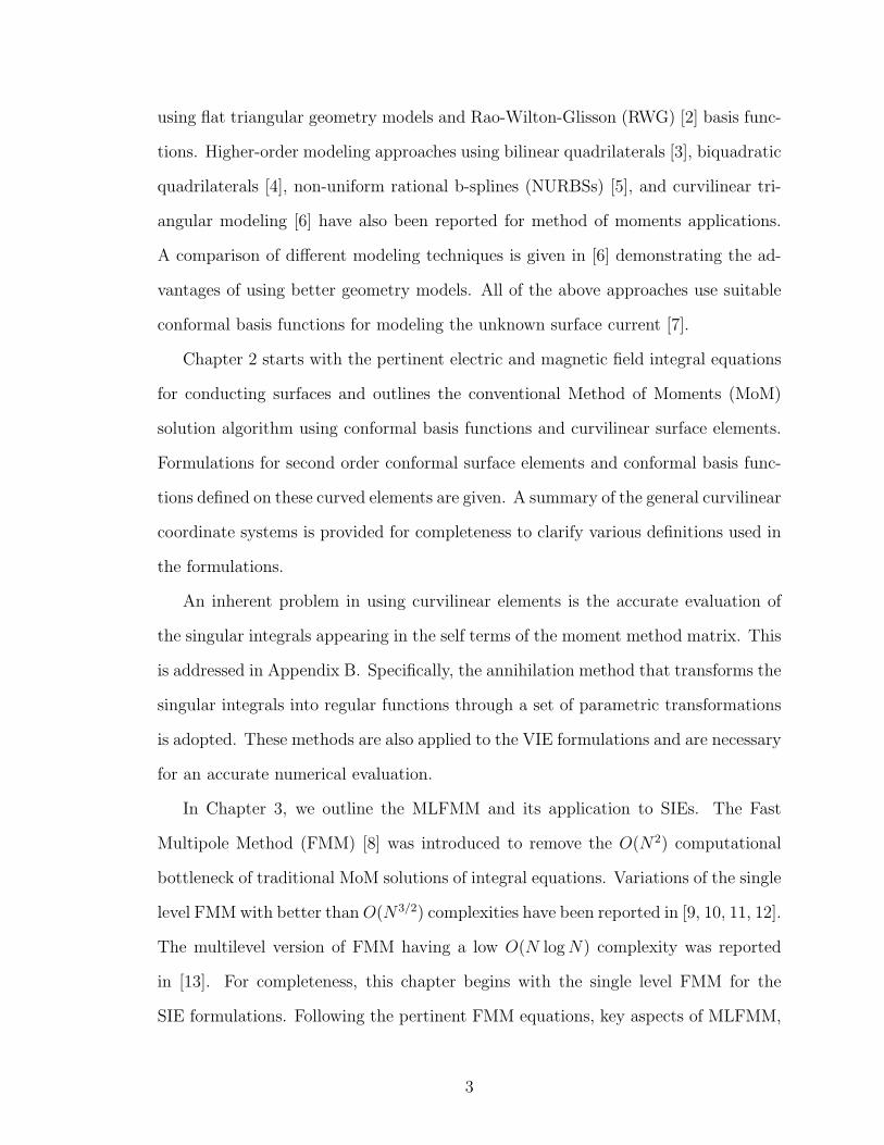
This thesis is aimed at developing fast algorithms based on the multilevel fast

multipole method (MLFMM) for composite structures. Previous developments and

applications of MLFMM dealt primarily with surface integral equations (SIEs). The

work presented in this thesis is the first to focus on the development and application

of MLFMM to volumetric composite structures. The key aspects of the thesis are:

1. Accurate geometry modeling. Accuracy is of most importance in large-

scale modeling due to numerical error accumulation as the matrix system size in-

creases. Also, geometry modeling accuracy is crucial as is the characterization of

1

material properties. This thesis is the first to develop fast solution algorithms for

large scale structures utilizing curvilinear surface and volume elements using integral

and hybrid integro-differential equation solvers.

2. Volumetric formulations. In the past, volume integral equations were not

attractive due to their excessive computational demands. In this thesis, we develop

fast algorithms for volumetric composite structures for the first time and demon-

strate that such algorithms are very attractive as compared to partial differential

equation (PDE) formulations. The use of curvilinear elements is a crucial aspect of

the formulation and is rather important when dealing with high contrast dielectric

coatings. As reported previously [1], these high contrast dielectrics require precise

geometry representation to maintain acceptable levels of accuracy. Also, different

approaches to solving volumetric integral equations (VIEs) are considered in terms of

efficiency and accuracy. These VIEs are implemented using a single vector unknown

within the volume and the MLFMM is applied for a numerically efficient solution

of such systems. A substantial contribution of the thesis is concerned with the spe-

cific volume formulations and how these lend themselves to accurate, efficient and

parallelizable algorithms.

As an alternative to VIE methods, we also implement a finite element-boundary

integral (FE-BI) solution using curvilinear elements. For the first time, the MLFMM

is implemented for carrying out the matrix-vector products in the boundary integral

portion of the matrix system. Thus, the resulting CPU requirements are O(N log N),

where N represents the size of the resulting matrix equation. Our study concludes

with a preliminary comparison of the hybrid FE-BI and VIE methods in terms of

solution accuracy and utilization of computer resources.

In Chapter 2, surface integral equations (SIEs) for conducting targets are reviewed

with particular emphasis on curvilinear elements for surface modeling. Traditionally,

solutions of SIEs for arbitrarily shaped conducting targets have mostly been studied

2

using flat triangular geometry models and Rao-Wilton-Glisson (RWG) [2] basis func-

tions. Higher-order modeling approaches using bilinear quadrilaterals [3], biquadratic

quadrilaterals [4], non-uniform rational b-splines (NURBSs) [5], and curvilinear tri-

angular modeling [6] have also been reported for method of moments applications.

A comparison of different modeling techniques is given in [6] demonstrating the ad-

vantages of using better geometry models. All of the above approaches use suitable

conformal basis functions for modeling the unknown surface current [7].

Chapter 2 starts with the pertinent electric and magnetic field integral equations

for conducting surfaces and outlines the conventional Method of Moments (MoM)

solution algorithm using conformal basis functions and curvilinear surface elements.

Formulations for second order conformal surface elements and conformal basis func-

tions defined on these curved elements are given. A summary of the general curvilinear

coordinate systems is provided for completeness to clarify various definitions used in

the formulations.

An inherent problem in using curvilinear elements is the accurate evaluation of

the singular integrals appearing in the self terms of the moment method matrix. This

is addressed in Appendix B. Specifically, the annihilation method that transforms the

singular integrals into regular functions through a set of parametric transformations

is adopted. These methods are also applied to the VIE formulations and are necessary

for an accurate numerical evaluation.

In Chapter 3, we outline the MLFMM and its application to SIEs. The Fast

Multipole Method (FMM) [8] was introduced to remove the O(N2) computational

bottleneck of traditional MoM solutions of integral equations. Variations of the single

level FMM with better than O(N3/2) complexities have been reported in [9, 10, 11, 12].

The multilevel version of FMM having a low O(N log N) complexity was reported

in [13]. For completeness, this chapter begins with the single level FMM for the

SIE formulations. Following the pertinent FMM equations, key aspects of MLFMM,

3

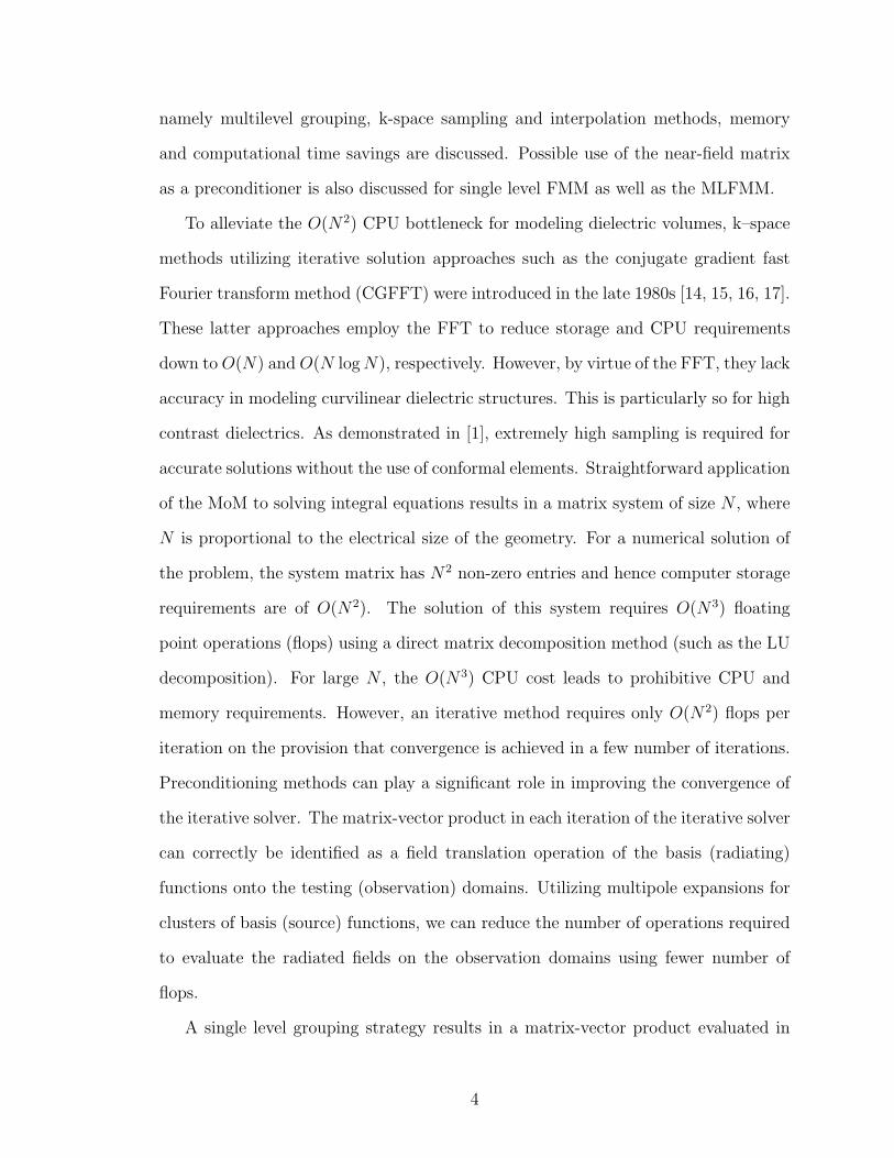
namely multilevel grouping, k-space sampling and interpolation methods, memory

and computational time savings are discussed. Possible use of the near-field matrix

as a preconditioner is also discussed for single level FMM as well as the MLFMM.

To alleviate the O(N2) CPU bottleneck for modeling dielectric volumes, k–space

methods utilizing iterative solution approaches such as the conjugate gradient fast

Fourier transform method (CGFFT) were introduced in the late 1980s [14, 15, 16, 17].

These latter approaches employ the FFT to reduce storage and CPU requirements

down to O(N) and O(N log N), respectively. However, by virtue of the FFT, they lack

accuracy in modeling curvilinear dielectric structures. This is particularly so for high

contrast dielectrics. As demonstrated in [1], extremely high sampling is required for

accurate solutions without the use of conformal elements. Straightforward application

of the MoM to solving integral equations results in a matrix system of size N , where

N is proportional to the electrical size of the geometry. For a numerical solution of

the problem, the system matrix has N2 non-zero entries and hence computer storage

requirements are of O(N2). The solution of this system requires O(N3) floating

point operations (flops) using a direct matrix decomposition method (such as the LU

decomposition). For large N , the O(N3) CPU cost leads to prohibitive CPU and

memory requirements. However, an iterative method requires only O(N2) flops per

iteration on the provision that convergence is achieved in a few number of iterations.

Preconditioning methods can play a significant role in improving the convergence of

the iterative solver. The matrix-vector product in each iteration of the iterative solver

can correctly be identified as a field translation operation of the basis (radiating)

functions onto the testing (observation) domains. Utilizing multipole expansions for

clusters of basis (source) functions, we can reduce the number of operations required

to evaluate the radiated fields on the observation domains using fewer number of

flops.

A single level grouping strategy results in a matrix-vector product evaluated in

4

O(N3/2) flops. This is the so called Fast Multipole Method (FMM). When the mul-

tipole expansions are utilized in a multilevel scheme (MLFMM), the resulting com-

plexity of the method can be reduced down to a remarkable O(N log N). Moreover,

since the whole MoM matrix need not be computed explicitly, the storage cost is

also reduced down to O(N3/2) for the single level FMM and down to O(N log N)

for the MLFMM. Similar to the FFT, the MLFMM is a fast and numerically exact

way of carrying out the matrix-vector product operation (which is essentially a field

translation operation) very efficiently.

We also examine the implementation of the MLFMM on distributed memory

parallel computers. Inter-processor communication issues are discussed for a general

purpose parallel implementation. With such parallel implementations, it is possible

to solve very large scale electromagnetics problems on low cost personal computer

clusters. This is only achievable with careful utilization of accurate higher-order

geometry models and adaptation of fast solvers such as the MLFMM.

In the third chapter of the thesis, we present the application of MLFMM to

hybrid FE-BI formulations for inhomogeneous problems. In this chapter, the FE-

BI method [18] using curvilinear volume and surface modeling [19] is outlined. In

addition to conformal surface elements, conformal volume elements are introduced.

These volume elements form the basis for the discretization of the VIEs that will be

outlined in the subsequent chapter. The extension of MLFMM to FE-BI systems

is presented as a totally new contribution. Strategies to reduce computer time and

memory as well as matrix conditioning issues for various choices of surface testing

functions are discussed.

Several methods have been used to formulate scattering and radiation problems

involving penetrable materials. The finite element method (FEM) [18] along with

various mesh truncation schemes is one of the most commonly used approaches.

Among these FEM methods, the FE-BI method [18, 19, 20, 21] provides an exact

5

means of truncating the FEM mesh, hence keeping the FEM domain small. This is

crucial in numerical simulations since the FEM method is prone to error propagation.

The necessity of using suitable geometry modeling schemes and basis functions in the

FE-BI formulation are also demonstrated, both in terms of solution accuracy and

convergence. As an alternative to partial differential equation methods, for problems

involving only homogeneous material regions, a surface integral equation formulation

can be used [22]. However, for regions with varying material properties a VIE must

be employed [23, 24]. In [23], cubic elements were used in this context and tetrahedral

elements were used in [24]. For curved geometries, tetrahedral elements [25, 26] are

more suitable than cubic elements due to their geometrical adaptability. Curved

hexahedral elements [19] are capable of modeling arbitrary geometries better than

tetrahedra. When dealing with thin layers, curved hexahedral elements are especially

more suitable since they avoid elongated tetrahedra which can lead to ill-conditioned

matrix systems.

So far, the FE-BI approach has not been exploited due to the excessive CPU and

memory requirements for large scale computations. Nevertheless, the MLFMM can

readily be incorporated to reduce the computational burden. Also, MLFMM may

allow for practical implementations of VIEs.

The last part of this thesis develops VIEs for composite targets. The modeling of

inhomogeneous structures has traditionally [27, 28] been carried out using equivalent

volume currents. Initial numerical implementations were done by Richmond [29] for

two-dimensional scatterers and later by Livesay and Chen [23] and Schaubert et.

al. [24] for three dimensions (see also Peterson [30] and Graglia et. al. [31]). Direct

use of equivalent currents to formulate integral equations is known to lead to 6 scalar

unknowns per location when both the permittivity and permeability are different

from those of free-space. As a result, volumetric structures over a wavelength per

linear dimension lead to very large numerical systems. Further, excessive sampling

6

requirements [1] for high contrast materials add to the computational burden. Thus,

numerical simulations have so far been focused on purely dielectric bodies (µr = 1).

To reduce the number of unknowns per volume location, two approaches can be

followed. One is to combine the equivalent electric and magnetic currents into a

single equivalent electric (or magnetic) current density Jeq (or Meq) [32]. Another is

to reduce the volume integral equation (VIE) into a volume-surface integral equation

(VSIE) as done in [1, 32] by invoking several integral identities and the divergence

theorem. The resulting integral equation involves differentiation of the permeability

within the inhomogeneous region. This differentiation may compromise the accuracy

of the formulation for high contrast dielectrics, and is further undesirable for piecewise

constant volumes.

The VIE development begins with a rigorous derivation of the appropriate integral

equation for efficient modeling of volume regions. In particular, we propose a VIE

which employs a single vector field unknown (instead of two vector unknowns as in the

past). The application of the MLFMM to this VIE is another important contribution

of this thesis. We present validation of the VIE and compare the solutions for various

composite targets using various higher-order volumetric basis functions. The perfor-

mance of the MLFMM solution is also demonstrated for electrically large dielectric

targets. Further, the VIE and FE-BI methods are compared both in terms of solution

accuracy and computational resources. The low computational cost and superior er-

ror performance of the VIE-MLFMM solutions as compared to the FE-BI-MLFMM

solutions are demonstrated.

The thesis concludes with a summary of major contributions and solution methods

for arbitrarily shaped inhomogeneous geometries.

7

CHAPTER 2

Surface Integral Equations

In this chapter, we outline the governing surface integral equations (SIEs) used to

formulate scattering by perfectly electrically conducting (PEC) bodies. The existence

and derivation of such integral equations starting with Maxwell’s equations will not

be discussed here, as they are quite standard in electromagnetic theory. The reader is

referred to referenced classical textbooks on advanced electromagnetic theory [27, 33].

Next, we first proceed with a description of the method of moments (MoM) employed

to solve the given integral equations. In doing so, we describe our geometry modeling

approach and specific basis functions for the discretization of the unknown induced

surface current density in the integral equations.

2.1 Surface Integral Equations for PEC Structures

In the presence of an external excitation, such as an incident electromagnetic field

due to an impressed source, the scattered field due to a PEC body (see Fig. 2.1) can

be calculated by replacing the object’s surface by an induced current source radiating

a scattered field in free-space, viz.

Escat(r) = iωµ0

∫

sdr′

[J(r′) +

1

k2∇′ · J(r′)∇

]g(r, r′) (2.1)

where Escat denotes the scattered field, ω is the frequency of operation, µ0 is the

free-space permeability, J(r) is the induced surface current on the PEC surface,

g(r, r′) = exp(ik|r − r′|)/4π|r − r′| is the free-space scalar Green’s function with

k being the wavenumber in the background medium. Throughout this thesis, an eiωt

8

iEiH

iksE

sHsk

n

ˆn t×t

Ω

(a) (b)

Figure 2.1. PEC scatterer in the presence of an external excitation. (a) Example surface mesh ofan ogive using conformal quadrilaterals, (b) Definition of the solid angle Ω.

time convention is assumed and suppressed.

The integral equation for this problem can be constructed by merely enforcing the

boundary condition for the tangential electric field component on the PEC surface s.

Enforcing the total tangential electric field to vanish on s, i.e. t · (Einc + Escat) = 0,

where t is the tangent unit vector to the body’s surface s (see Fig. 2.1 (a)), yields the

so called electric field integral equation (EFIE)

t ·∫

sdr′G(r, r′) · J(r′) =

i

kηt · Einc(r), (2.2)

where Einc(r) is the incident electric field and η =√

µ/ε is the impedance of the

background medium. Here, we have equivalently adopted the more compact dyadic

Green’s function representation with

G(r, r′) =[I +

1

k2∇∇

]g(r, r′). (2.3)

Similarly, using the boundary condition J = n× (Hinc + Hscat) 1, it is possible to

derive the so called magnetic field integral equation (MFIE) valid for closed scatterers

and given by

−T n× J(r) +∫

s− dr′J(r′)×∇g(r, r′) = n×Hinc(r). (2.4)

1The enforced boundary condition is the usual J = n× (H+ −H−), where H+ = Hinc + Hscat

is the exterior field and H− = 0 within the PEC body.

9

In this, T = 1−Ω/4π and Ω is the solid angle subtended by the observation point (see

Fig. 2.1 (b)) and the bar through the integral sign represents the principal value

excluding the observation point r. For smooth surfaces, Ω = 2π and hence T = 1/2.

Also, in the above, n denotes the normal vector on the closed surface S pointing

outward as shown in Fig. 2.1 (a).

For arbitrary geometries, the solution of the above EFIE and MFIE must be

carried out numerically. The MoM is the most popular numerical solution approach.

It is based in expanding the unknown J using a suitable set of basis functions. Below,

we present the MoM solution of (2.2) and (2.4) starting by introducing the geometry

modeling approach and basis functions.

2.2 Geometry Modelling and Basis Functions

Real-life electromagnetics problems almost always involve arbitrary geometries com-

posed of quite complicated components having arbitrary curvatures and intricate de-

tail. A military aircraft, for example, has a streamlined fuselage with very thin wings

attached along with attached munition and various antennas. To mathematically

represent such complicated structures, one must resort to simpler geometry model-

ing techniques. Among several popular and powerful modeling methods [34, 35], we

use parametric elements to model scatterer geometries. As compared to flat facet

modeling, conformal elements lower the solution error by improving geometry repre-

sentations. Below, we outline the mathematical basis for parametric surface modeling

and present the specific modeling technique used throughout this work.

Parametric representation is the mapping of a unit element (be it a triangle or a

square or a general multilateral) in a parametric (u, v) space through the transfor-

mation

r = r(u, v). (2.5)

Usually such a parametric representation is constructed as a Cartesian product of

10

one-dimensional transformations. Fig. 2.2 depicts several one-dimensional parametric

mappings. Basically, the parametric curve in the (x, y, z) space is mapped on a unit

Polynomial interpolation

Bezier curve and its defining polygon

B-splines:Smoothly blended

Bezier curves

NURBSFamily of curves

for various weights

r1

r2

r3

r1

r2

r3

r1

r2r3

r4

r5

(r1,w1)

(r2,w2)

(r3,w3) (r4,w4)

(r5,w5)

u1 u2 u3

u1 u2 u3

u1 u2 u3

Figure 2.2. Examples of parametric mappings.

straight line in the parametric (u) space through r = r(u). Likewise, a curvilinear

quadrilateral element in the (x, y, z) space is the image of the unit square in the (u, v)

space through a different form of (2.5). Needless to say, (2.5) is the mathematical

representation of the curvilinear element in the (x, y, z) coordinates. Several common

elements are depicted in Fig. 2.3.

Flat triangle Quadratic triangle

Bi-linear quadrilateral Bi-quadratic quadrilateral

Figure 2.3. Examples of surface elements.

11

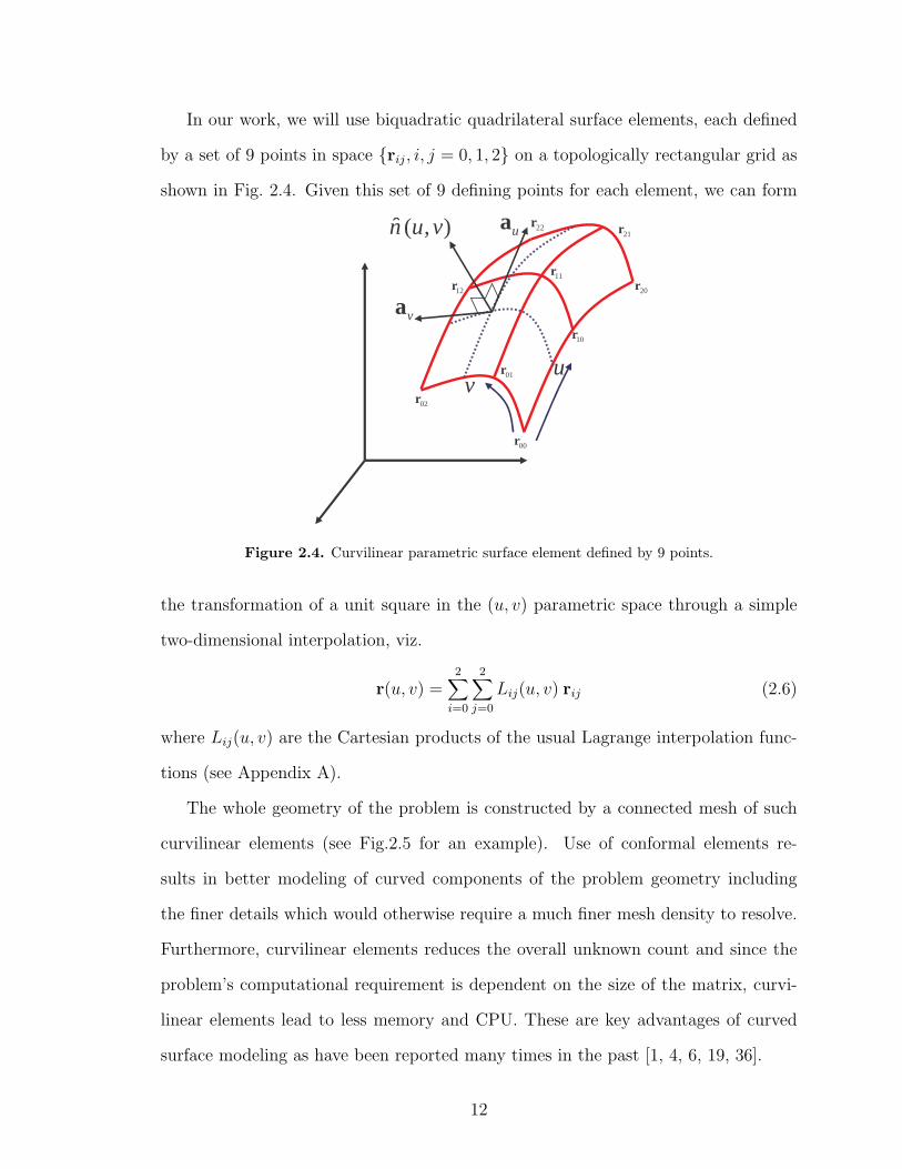
In our work, we will use biquadratic quadrilateral surface elements, each defined

by a set of 9 points in space rij, i, j = 0, 1, 2 on a topologically rectangular grid as

shown in Fig. 2.4. Given this set of 9 defining points for each element, we can form

10r

20r11r

21r

12r

22r

00r

01r

02r

uv

ua

va

),(ˆ vun

Figure 2.4. Curvilinear parametric surface element defined by 9 points.

the transformation of a unit square in the (u, v) parametric space through a simple

two-dimensional interpolation, viz.

r(u, v) =2∑

i=0

2∑

j=0

Lij(u, v) rij (2.6)

where Lij(u, v) are the Cartesian products of the usual Lagrange interpolation func-

tions (see Appendix A).

The whole geometry of the problem is constructed by a connected mesh of such

curvilinear elements (see Fig.2.5 for an example). Use of conformal elements re-

sults in better modeling of curved components of the problem geometry including

the finer details which would otherwise require a much finer mesh density to resolve.

Furthermore, curvilinear elements reduces the overall unknown count and since the

problem’s computational requirement is dependent on the size of the matrix, curvi-

linear elements lead to less memory and CPU. These are key advantages of curved

surface modeling as have been reported many times in the past [1, 4, 6, 19, 36].

12

Figure 2.5. Generic VFY218 aircraft modelled by quadrilateral patches.

Once the geometry is mathematically represented with a mesh of connected el-

ements, the next step is to define basis functions conformal to these elements for

representing the unknown induced surface current density. This allows us to convert

the SIE into a matrix system through the MoM procedure. The intricate relation-

ships between the mesh density, problem size, and solution time will be discussed in

detail later in the context of fast solution algorithms.

2.3 MoM Procedure for EFIE

To discretize and solve (2.2) for the unknown surface current, we introduce a linear

representation of the unknown J in terms of known basis functions with unknown

coefficients. Mathematically, this corresponds to projecting the vector function J

onto a finite dimensional sub-space spanned by the set of basis j1, j2, ..., jN. We

will not repeat the details of the general MoM procedure here. Instead, we will only

outline the specific MoM solution for the governing integral equation.

The basis functions for the induced surface electric currents are constructed as

a generalization of rooftop basis functions defined on a pair of flat rectangular do-

13

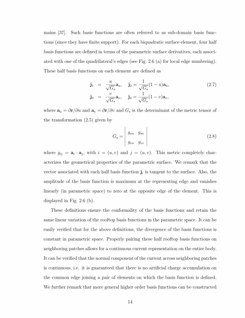
mains [37]. Such basis functions are often referred to as sub-domain basis func-

tions (since they have finite support). For each biquadratic surface element, four half

basis functions are defined in terms of the parametric surface derivatives, each associ-

ated with one of the quadrilateral’s edges (see Fig. 2.6 (a) for local edge numbering).

These half basis functions on each element are defined as

j1 =u√Gs

au, j2 =1√Gs

(1− u)au, (2.7)

j3 =v√Gs

av, j4 =1√Gs

(1− v)av,

where au = ∂r/∂u and av = ∂r/∂v and Gs is the determinant of the metric tensor of

the transformation (2.5) given by

Gs =

∣∣∣∣∣∣∣∣

guu guv

gvu gvv

∣∣∣∣∣∣∣∣(2.8)

where gij = ai · aj, with i = (u, v) and j = (u, v). This metric completely char-

acterizes the geometrical properties of the parametric surface. We remark that the

vector associated with each half basis function ji is tangent to the surface. Also, the

amplitude of the basis function is maximum at the representing edge and vanishes

linearly (in parametric space) to zero at the opposite edge of the element. This is

displayed in Fig. 2.6 (b).

These definitions ensure the conformality of the basis functions and retain the

same linear variation of the rooftop basis functions in the parametric space. It can be

easily verified that for the above definitions, the divergence of the basis functions is

constant in parametric space. Properly pairing these half rooftop basis functions on

neighboring patches allows for a continuous current representation on the entire body.

It can be verified that the normal component of the current across neighboring patches

is continuous, i.e. it is guaranteed that there is no artificial charge accumulation on

the common edge joining a pair of elements on which the basis function is defined.

We further remark that more general higher order basis functions can be constructed

14

if the linear variations in (2.7) are replaced by appropriate functions. However, the

accuracy of such a representation should be correlated to the accuracy of the actual

geometry modeling. That is, one should not pursue a higher-order representation of

the current density aiming to improve solution accuracy if the surface representation is

not equally accurate. Nevertheless, with accurate geometry representations, higher-

order basis functions have been reported to generate smaller MoM systems hence

require less computational resources [38].

For completeness, we note here the basic differential operations associated with

parametric surfaces. The surface gradient of a scalar function φ(u, v) is given by

∇sφ(u, v) = guu ∂φ

∂uau + guv ∂φ

∂uav + gvu ∂φ

∂vau + gvv ∂φ

∂vav (2.9)

where gij, i = (u, v) and j = (u, v) are the elements of the inverse metric tensor. Also,

the surface divergence of a vector function f(u, v) = fuau + fvav is given by

∇s · f(u, v) = guu ∂f

∂u· au + guv ∂f

∂u· av + gvu ∂f

∂v· au + gvv ∂f

∂v· av (2.10)

=1√Gs

(∂(fu

√Gs)

∂u+

∂(fv

√Gs)

∂v

).

Figure 2.6 depicts two quadrilaterals, each arbitrarily oriented, sharing a common

edge. As mentioned, each basis function is defined on a pair of adjoining elements, and

the definition (2.7) ensures the continuity of the normal current density component

across the common edge. For the depicted situation, the half basis function defined

on element 1 will be j(1)2 = − 1√

Gs(1− u)au where the superscript denotes the element

number and the subscript refers to the local edge number. Similarly, the half basis

function on element 2 is j(2)3 = − v√

Gsav, where the minus signs are introduced to

correct for the direction of current flow. The normal component of j(1)2 across the

common edge can be found using the tangential and normal unit vectors to that

edge, i.e.

t‖ =1√gvv

av, t⊥ = t‖ × n =1√

Gsgvv

[gvvau − guvav] . (2.11)

15

Element 1

Element 2

u v

u

vn

n

1

2

3

4

1

23

4

(1)2j

(2)3j

t

t⊥

−1

0

1

2

3

−2

−1

0

1

2−2

−1.5

−1

−0.5

0

0.5

1

1.5

2

(a) (b)

Figure 2.6. Constructing basis functions: (a) Two patches forming the support of basis func-tion associated with the common edge, (b) Quiver plot of the conformal basis (length of arrows isassociated with the amplitude of the basis function).

Using (2.11), the normal component of j(1)2 and j

(2)3 are given by

t⊥ · j(1)2 =

1√gvv(u = 1, v)

(2.12)

t⊥ · j(2)3 =

1√guu(u, v = 0)

. (2.13)

Since both values only depend on the differential length over the common edge, the

normal components of both halves of the basis function will be equal, indicating

continuity of that component. We can also verify that the surface divergence on both

halves are ∇s ·j(1)2 = 1/

√Gs and ∇s ·j(2)

3 = −1/√

Gs, implying constant surface charge

σ = ∇s · j in the parametric space (i.e. σds/dudv = ±1)2.

To proceed with the MoM implementation, we assume that the unknown function

J is a linear combination of the defined basis functions as J(r) =∑N

i=1 xiji(r), where

xi are the unknown coefficients of the expansion. When this expansion is substituted

in (2.2), we get

t ·∫

sdr′G(r, r′) ·

N∑

i=1

xiji(r′) =

i

kηt · Einc(r) (2.14)

2ds =√

Gsdudv

16

or equivalently,N∑

i=1

xit ·∫

sdr′G(r, r′) · ji(r′) =

i

kηt · Einc(r). (2.15)

To find the unknown coefficients xi, we employ Galerkin’s testing (for Galerkin’s

testing tj = bj) to obtain

N∑

i=1

xi

∫

sdrtj(r) ·

∫

sdr′G(r, r′) · ji(r′) =

i

kη

∫

sdrtj(r) · Einc(r). (2.16)

For j = 1, ..., N , this leads to N linear equations for the solution of the N unknowns.

Equation (2.16) can thus be cast into a matrix system as [Z]x = b, where

Zji =∫

sdrtj(r) ·

∫

sdr′G(r, r′) · ji(r′) (2.17)

and

bj =i

kη

∫

sdrtj(r) · Einc(r) (2.18)

being the excitation vector due to the incident wave Einc(r). Solution of this system

provides the unknown coefficients of the expansion J(r) =∑N

i=1 xiji(r) for the induced

surface current density.

The double surface integrals in the matrix element in (2.17) need to be numerically

evaluated using a suitable quadrature rule. Since each basis and testing function is

defined on pairs of elements it is advantageous to compute the contributions to the

matrix entries from pairs of basis and testing domains (i.e. compute element sub-

matrices). Subsequently, these contributions are added into the actual matrix using

the connectivity of the mesh, much like it is done in standard finite element method.

That is, the 4 × 4 element matrix Zkl between the lth source element and the kth

testing element (see Fig. 2.7) is computed in the parametric (u, v) and (u′, v′) unit

squares as

Zkl =∫ 1

0

∫ 1

0drt′j(r) ·

∫ 1

0

∫ 1

0dr′G(r, r′) · j′i(r′) (2.19)

where t′j denotes each of the 4 half-testing functions on element k and j′i denotes each

of the 4 half-basis functions on element l. Using dr =√

Gsdudv and dr′ =√

G′sdu′dv′,

17

Source patch Testing patch

u v u

v

n n

1

2

3

41

23

4

11Z

42Z

33Z

34Z

11 12 13 14

21 22 23 24

31 32 33 34

41 42 43 44

el

Z Z Z Z

Z Z Z ZZ

Z Z Z Z

Z Z Z Z

=

Figure 2.7. Illustration for the computation of the element matrices.

we can rewrite (2.19) as

Zkl =∫

sk

√Gsdudvt′j(r) ·

∫

sl

√G′

sdu′dv′G(r, r′) · j′i(r′). (2.20)

Recalling the definitions of basis functions in (2.7), we realize that the normalization

factor 1/√

Gs need never actually be computed since it is cancelled by the Jaco-

bian (i.e. the differential area factor) in (2.20). The hyper-singularity in (2.20) can

be relaxed through the use of the divergence theorem. When we explicitly state the

dyadic Green’s function in (2.17), we obtain

Zji =∫

sdrtj(r) ·

[∫

sdr′g(r, r′)ji(r′) +

1

k2

∫

sdr′∇∇g(r, r′) · ji(r′)

](2.21)

or equivalently,

Zji =∫

sdrtj(r) ·

[∫

sdr′g(r, r′)ji(r′)− 1

k2∇

∫

sdr′∇′g(r, r′) · ji(r′)

]. (2.22)

We can transfer the ∇′ operator to the basis function using the vector identity ∇′ ·(gji) = ∇′g · ji + g∇′ · ji and the divergence theorem. These manipulations result in

Zji =∫

sdrtj(r) ·

[∫

sdr′g(r, r′)ji(r′) (2.23)

− 1

k2∇

∫

sdr′ ∇′ · [g(r, r′)ji(r′)]− g(r, r′)∇′ · ji(r′)

]

=∫

sdrtj(r) ·

[∫

sdr′g(r, r′)ji(r′) +

1

k2∇

∫

sdr′g(r, r′)∇′ · ji(r′)

]

−∫

sdrtj(r) ·

[1

k2∇

∮

cdr′ · g(r, r′)ji(r′)

]

18

where dr′ of the closed line integral is the normal differential vector to the boundary

c of the basis domain s (see Fig. 2.8). Since dr′ is always perpendicular to the basis

function ji(r′), this integral vanishes, hence

Zji =∫

sdrtj(r) ·

[∫

sdr′g(r, r′)ji(r′) +

1

k2∇

∫

sdr′g(r, r′)∇′ · ji(r′)

]. (2.24)

We can again use the divergence theorem ∇ · (φA) = ∇φ ·A + φ∇ ·A on the second

term in the above integral with A = tj(r) and φ =∫s dr′g(r, r′)∇′ · ji(r′) and rewrite

(2.24) as

Zji =∫

sdrtj(r) ·

∫

sdr′g(r, r′)ji(r′) (2.25)

+1

k2

∮

cdr ·

[tj(r)

∫

sdr′g(r, r′)∇′ · ji(r′)

]

− 1

k2

∫

sdr∇ · tj(r)

∫

sdr′g(r, r′)∇′ · ji(r′)

where dr is the normal differential vector to the boundary c of the testing domain

s (as depicted in Fig. 2.8). Since dr and tj(r) are always perpendicular to each other

Differential element on the boundary c of the surface s

n

c s= ∂s

dr

dr

dr

dr

Figure 2.8. Application of the divergence theorem on the testing function.

on the outer boundary c, the line integral in (2.25) is identically zero, yielding the

desired equation

Zji =∫

sdrtj(r) ·

∫

sdr′g(r, r′)ji(r′)− 1

k2

∫

sdr∇ · tj(r)

∫

sdr′g(r, r′)∇′ · ji(r′). (2.26)

After this manipulation, both of the integrals in (2.25) have a first order singularity

when the source and testing domains overlap. This is an integrable singularity, nev-

ertheless care must be taken in numerically evaluating the singular kernels. We have

19

used an annihilation technique for integrating the singularity in the source integral for

the self term (i.e. when testing and basis domains overlap). This technique is outlined

in the Appendix B. In the numerical computation of (2.26), we have used Gaussian

quadrature. Several orders of Gaussian quadrature points on the unit square in the

(u, v) parametric space are depicted in Fig. 2.9.

−1 −0.5 0 0.5 1−1

−0.5

0

0.5

1

−1 −0.5 0 0.5 1−1

−0.5

0

0.5

1

−1 −0.5 0 0.5 1−1

−0.5

0

0.5

1

Figure 2.9. Several orders of Gaussian quadrature points for −1 < u < 1 and −1 < v < 1.

Once the elements of the matrix equation are accurately computed, the matrix

system must be solved to get the unknown coefficients xi for i = 1, ..., N. To do so,

one can use a direct solution method, such as Gaussian elimination (or LU decompo-

sition), which however is associated with O(N3) computational cost. Alternatively,

an iterative solution method [39] with O(N2) complexity per iteration can be used.

For the latter case, the hope is to achieve convergence in a few iterations. Several

preconditioning methods can also be utilized to achieve quick convergence [40]. In

the next section, we present examples and validations of the outlined methodology.

Since the MoM is a well-established method for solving integral as well as partial

differential equations [41], and since an error analysis for the above procedure is well

beyond the scope of this work (and is probably impossible for an arbitrary geometry),

here we only demonstrate the convergence of the numerical results as the mesh den-

sity is increased. However, as a rule of thumb, a λ/10 element size will be adopted.

This rule aims at accurately resolving variations in the induced surface current using

rooftop (linear) basis functions. This is demonstrated below as the results are accu-

20

rate to within less than 1 % for λ/10 discretization sizes for all test geometries. We

also demonstrate below the superior geometry modeling capability of the outlined

curvilinear elements.

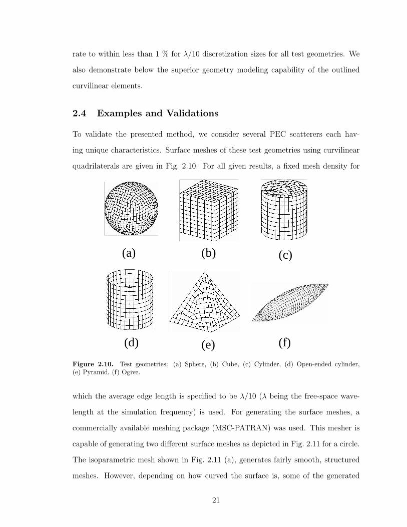
2.4 Examples and Validations

To validate the presented method, we consider several PEC scatterers each hav-

ing unique characteristics. Surface meshes of these test geometries using curvilinear

quadrilaterals are given in Fig. 2.10. For all given results, a fixed mesh density for

(a) (b) (c)

(d) (e) (f)

Figure 2.10. Test geometries: (a) Sphere, (b) Cube, (c) Cylinder, (d) Open-ended cylinder,(e) Pyramid, (f) Ogive.

which the average edge length is specified to be λ/10 (λ being the free-space wave-

length at the simulation frequency) is used. For generating the surface meshes, a

commercially available meshing package (MSC-PATRAN) was used. This mesher is

capable of generating two different surface meshes as depicted in Fig. 2.11 for a circle.

The isoparametric mesh shown in Fig. 2.11 (a), generates fairly smooth, structured

meshes. However, depending on how curved the surface is, some of the generated

21

elements may be severely distorted, making the mesh unsuitable for numerical so-

lutions due to matrix ill-conditioning. On the other hand, the paver mesh (shown

in Fig. 2.11 (b)) generates an unstructured mesh and is rid of the limitations of the

isoparametric mesh. Below, we provide some numerical solutions using both kinds

of meshes for the same geometry, and demonstrate that both meshes provide compa-

rable accuracy. The first test geometry is a PEC sphere of radius 1 m, as depicted

(a) (b)

Figure 2.11. Two different meshing methods for a circle: (a) Isoparametric mesh, (b) Paver mesh.

in Fig. 2.10 (a). This is a unique 3-dimensional geometry for which an analytical

solution (Mie series) exists. Hence, it provides a reference solution to be used for

evaluating the numerical solution error. The frequency of the incident electromag-

netic field is 300 MHz. The bistatic RCS results for both polarizations of the incident

0 45 95 135 180−15

−10

−5

0

5

10

15

20

25

30

Observation angle θ (degrees)

Bis

tatic

RC

S (

dB/λ

2 )

EFIE Solution for Paver Mesh

MieMoM

0 45 95 135 180−15

−10

−5

0

5

10

15

20

25

30

Observation angle θ (degrees)

Bis

tatic

RC

S (

dB/λ

2 )

EFIE Solution for Isoparametric Mesh

MieMoM

Figure 2.12. Bistatic scattering results for the sphere using the EFIE.

field using the paver and isoparametric meshes are shown in Fig. 2.12. Owing to the

22

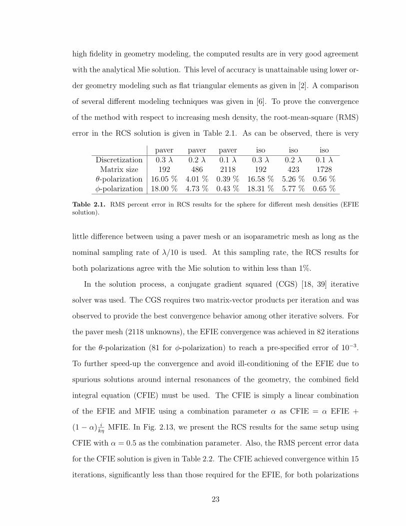
high fidelity in geometry modeling, the computed results are in very good agreement

with the analytical Mie solution. This level of accuracy is unattainable using lower or-

der geometry modeling such as flat triangular elements as given in [2]. A comparison

of several different modeling techniques was given in [6]. To prove the convergence

of the method with respect to increasing mesh density, the root-mean-square (RMS)

error in the RCS solution is given in Table 2.1. As can be observed, there is very

paver paver paver iso iso isoDiscretization 0.3 λ 0.2 λ 0.1 λ 0.3 λ 0.2 λ 0.1 λMatrix size 192 486 2118 192 423 1728

θ-polarization 16.05 % 4.01 % 0.39 % 16.58 % 5.26 % 0.56 %φ-polarization 18.00 % 4.73 % 0.43 % 18.31 % 5.77 % 0.65 %

Table 2.1. RMS percent error in RCS results for the sphere for different mesh densities (EFIEsolution).

little difference between using a paver mesh or an isoparametric mesh as long as the

nominal sampling rate of λ/10 is used. At this sampling rate, the RCS results for

both polarizations agree with the Mie solution to within less than 1%.

In the solution process, a conjugate gradient squared (CGS) [18, 39] iterative

solver was used. The CGS requires two matrix-vector products per iteration and was

observed to provide the best convergence behavior among other iterative solvers. For

the paver mesh (2118 unknowns), the EFIE convergence was achieved in 82 iterations

for the θ-polarization (81 for φ-polarization) to reach a pre-specified error of 10−3.

To further speed-up the convergence and avoid ill-conditioning of the EFIE due to

spurious solutions around internal resonances of the geometry, the combined field

integral equation (CFIE) must be used. The CFIE is simply a linear combination

of the EFIE and MFIE using a combination parameter α as CFIE = α EFIE +

(1 − α) ikη

MFIE. In Fig. 2.13, we present the RCS results for the same setup using

CFIE with α = 0.5 as the combination parameter. Also, the RMS percent error data

for the CFIE solution is given in Table 2.2. The CFIE achieved convergence within 15

iterations, significantly less than those required for the EFIE, for both polarizations

23

0 45 95 135 180−15

−10

−5

0

5

10

15

20

25

30

Observation angle θ (degrees)

Bis

tatic

RC

S (

dB/λ

2 )

CFIE(α=0.5) Solution for Paver Mesh

MieMoM

0 45 95 135 180−15

−10

−5

0

5

10

15

20

25

30

Observation angle θ (degrees)

Bis

tatic

RC

S (

dB/λ

2 )

CFIE(α=0.5) Solution for Isoparametric Mesh

MieMoM

Figure 2.13. Bistatic scattering results for the sphere using the CFIE with (α = 0.5).

paver paver paver iso iso isoDiscretization 0.3 λ 0.2 λ 0.1 λ 0.3 λ 0.2 λ 0.1 λMatrix size 192 486 2118 192 423 1728

θ-polarization 16.04 % 5.08 % 0.82 % 16.01 % 5.70 % 1.00 %φ-polarization 16.26 % 4.23 % 0.67 % 16.46 % 5.05 % 0.82 %

Table 2.2. RMS percent error in RCS results for the sphere for different mesh densities (CFIEsolution).

and for an error of less than 10−3. In Fig. 2.14, we depict the RCS results using

the MFIE. The MFIE is also prone to spurious solutions and unlike the EFIE, the

MFIE fails even to generate correct far-field results. The results given in Fig. 2.14

are provided for completeness and the MFIE will not further be considered for the

other test geometries.

The next test geometry is a cube of side length 1 m. For the cube, there is

no advantage in using curvilinear elements. Nevertheless, since flat facets can be

modeled equally well using curvilinear elements, they will be used for the cube as

well. This geometry was chosen as a test case for representing targets with sharp

edges. The bistatic RCS of the cube for both incident field polarizations using the

EFIE and the CFIE are given in Fig. 2.15. Since these is no analytical solution for

this problem, we depict two solutions for two different sampling rates. The agreement

for both integral equations is excellent and the RMS error between the two solutions

24

0 45 95 135 180−15

−10

−5

0

5

10

15

20

25

30

Observation angle θ (degrees)

Bis

tatic

RC

S (

dB/λ

2 )

MFIE Solution for Paver Mesh

MieMoM

0 45 95 135 180−15

−10

−5

0

5

10

15

20

25

30

Observation angle θ (degrees)

Bis

tatic

RC

S (

dB/λ

2 )

MFIE Solution for Isoparametric Mesh

MieMoM

Figure 2.14. Bistatic scattering results for the sphere using the MFIE

are 0.38%− 0.37% for the EFIE and 0.48%− 0.53% for the CFIE. Nominal sampling

0 45 95 135 180−30

−20

−10

0

10

20

Observation angle θ (degrees)

Bis

tatic

RC

S (

dB/λ

2 )

EFIE Solution with Different Discretizations

0.075 λ0.100 λ

0 45 95 135 180−30

−20

−10

0

10

20

Observation angle θ (degrees)

Bis

tatic

RC

S (

dB/λ

2 )

CFIE(α=0.5) Solution with Different Discretizations

0.075 λ0.100 λ

Figure 2.15. Bistatic scattering results for the cube using the EFIE and the CFIE (α = 0.5).

resulted in 1200 unknowns and convergence was achieved within 137− 102 iterations

for the EFIE and 13 iterations for the CFIE. The over-sampled mesh (at 0.075λ)

generated 2028 unknowns and the EFIE converged in 116 iterations as compared to

14 CFIE iterations.

The cylinder is the third test geometry to be considered here. This geometry

requires both flat and curved elements for modeling. The RCS results for the cylinder

are given in Fig. 2.16. Again, the convergence of the RCS curves with increasing

mesh density is excellent. The difference between the two solutions with a paver

mesh are 0.31% − 0.34% and 0.47% − 0.50% for the EFIE and CFIE, respectively.

25

0 45 95 135 180−20

−10

0

10

20

Observation angle θ (degrees)

Bis

tatic

RC

S (

dB/λ

2 )

EFIE Solution with Different Discretizations

0.075 λ0.100 λ

0 45 95 135 180−20

−10

0

10

20

Observation angle θ (degrees)

Bis

tatic

RC

S (

dB/λ

2 )

CFIE(α=0.5) Solution with Different Discretizations

0.075 λ0.100 λ

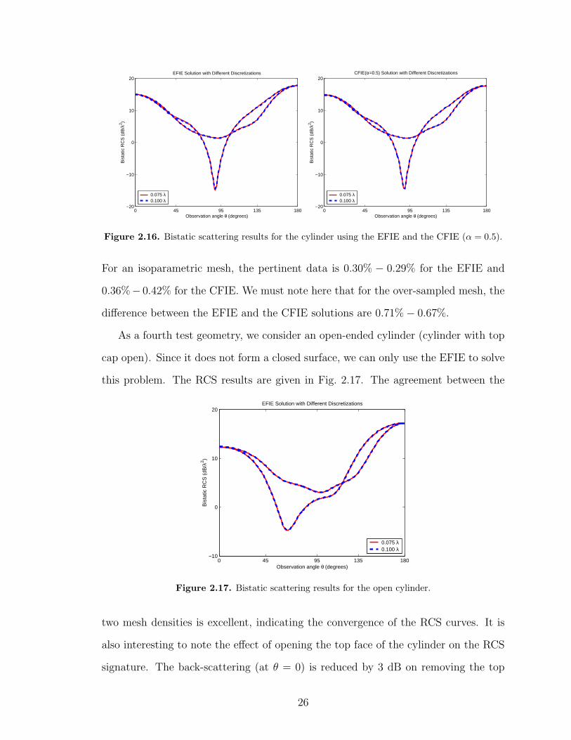
Figure 2.16. Bistatic scattering results for the cylinder using the EFIE and the CFIE (α = 0.5).

For an isoparametric mesh, the pertinent data is 0.30% − 0.29% for the EFIE and

0.36%− 0.42% for the CFIE. We must note here that for the over-sampled mesh, the

difference between the EFIE and the CFIE solutions are 0.71%− 0.67%.

As a fourth test geometry, we consider an open-ended cylinder (cylinder with top

cap open). Since it does not form a closed surface, we can only use the EFIE to solve

this problem. The RCS results are given in Fig. 2.17. The agreement between the

0 45 95 135 180−10

0

10

20

Observation angle θ (degrees)

Bis

tatic

RC

S (

dB/λ

2 )

EFIE Solution with Different Discretizations

0.075 λ0.100 λ

Figure 2.17. Bistatic scattering results for the open cylinder.

two mesh densities is excellent, indicating the convergence of the RCS curves. It is

also interesting to note the effect of opening the top face of the cylinder on the RCS

signature. The back-scattering (at θ = 0) is reduced by 3 dB on removing the top

26

cover of the cylinder.

Fig. 2.18 depicts the bistatic RCS of the pyramid shown in Fig. 2.10 (e), our fifth

geometry. Two different results are given to ensure mesh convergence. As compared

0 45 95 135 180−20

−10

0

10

20

Observation angle θ (degrees)

Bis

tatic

RC

S (

dB/λ

2 )

EFIE Solution with Different Discretizations

0.075 λ0.100 λ

0 45 95 135 180−20

−10

0

10

20

Observation angle θ (degrees)

Bis

tatic

RC

S (

dB/λ

2 )

CFIE(α=0.5) Solution with Different Discretizations

0.075 λ0.100 λ

Figure 2.18. Bistatic scattering results for the pyramid using the EFIE and the CFIE (α = 0.5).

to the closed cylinder, there is more than 10 dB reduction in the back-scatter return.

The paver and isoparametric meshes resulted in 704 and 960 unknowns at λ/10

sampling and 1222 and 1766 unknowns at λ/10 sampling, respectively. The EFIE

converged in 69 CGS iterations and the CFIE converged in 15 CGS iterations for the

704 unknown problem. For the over-sampled case (1766 unknowns), 145− 142 EFIE

iterations were executed as compared to 24 CFIE iterations.

Our sixth and final test geometry is from the Electromagnetic Code Consor-

tium (EMCC). The ogive geometry has a curved elongated body and two sharp tips.

The sharp tips present a modeling challenge and consequently the geometry is well-

suited for validating electromagnetic computer codes being developed by research

centers and government agencies using different solution approaches. The computed

bistatic RCS results are shown in Fig. 2.19. The dynamic RCS range of the curves

is about 50 dB and the back-scattering return is clearly very low. In spite of this

large dynamic range, the predicted results for both polarizations agree very well for

the two mesh densities. The EFIE convergence was achieved in 313− 363 iterations

27

0 45 95 135 180−40

−30

−20

−10

0

10

20

Observation angle θ (degrees)

Bis

tatic

RC

S (

dB/λ

2 )

EFIE Solution with Different Discretizations

0.075 λ0.100 λ

0 45 95 135 180−40

−30

−20

−10

0

10

20

Observation angle θ (degrees)

Bis

tatic

RC

S (

dB/λ

2 )

CFIE(α=0.5) Solution with Different Discretizations

0.075 λ0.100 λ

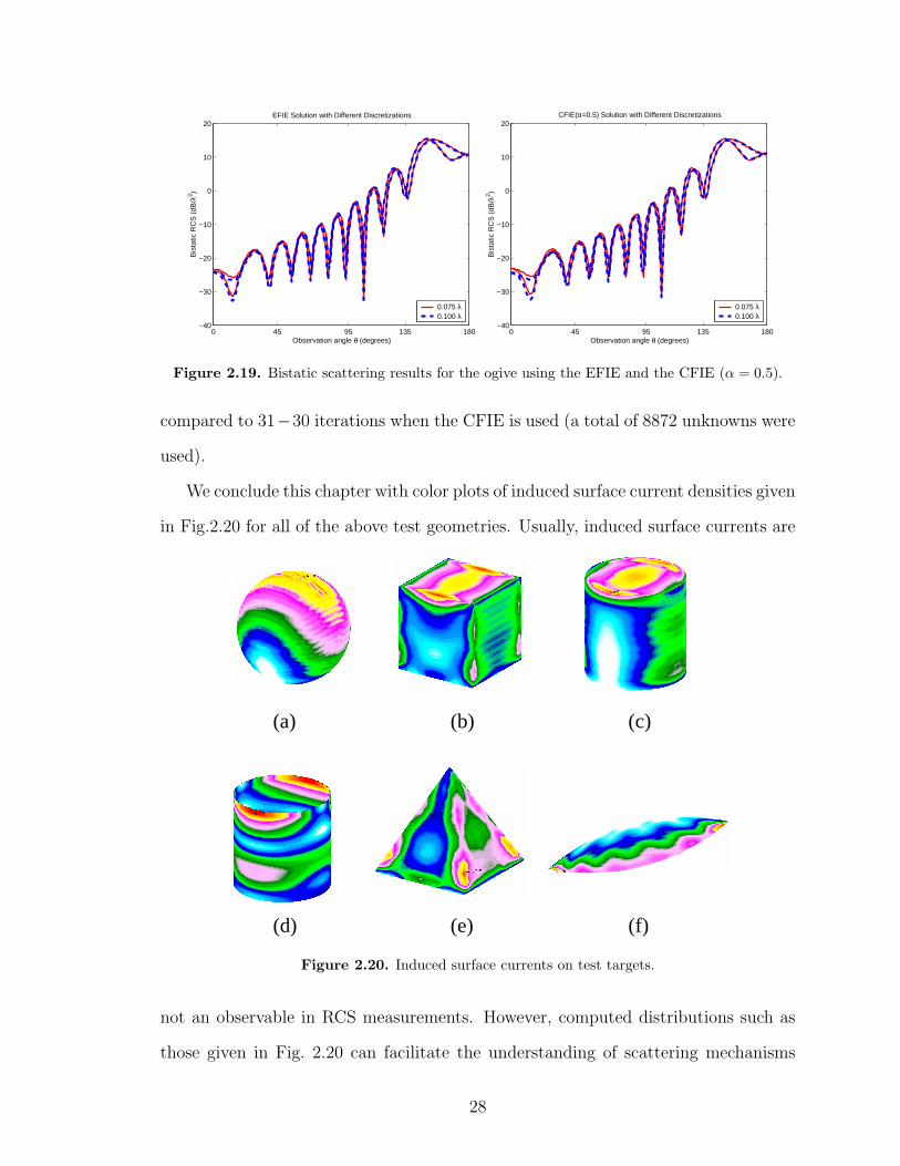
Figure 2.19. Bistatic scattering results for the ogive using the EFIE and the CFIE (α = 0.5).

compared to 31−30 iterations when the CFIE is used (a total of 8872 unknowns were

used).

We conclude this chapter with color plots of induced surface current densities given

in Fig.2.20 for all of the above test geometries. Usually, induced surface currents are

(a) (b) (c)

(d) (e) (f)

Figure 2.20. Induced surface currents on test targets.

not an observable in RCS measurements. However, computed distributions such as

those given in Fig. 2.20 can facilitate the understanding of scattering mechanisms

28

and is necessary in designing low RCS targets.

For realistic structures with sharp edges and tips as well as curved surfaces, the

problem size quickly reaches the limits of a given computing platform. As an example,

the EFIE ogive system required 630 MBytes of computer memory and 45 minutes

on a Pentium III processor. To remove the O(N2) memory and CPU bottlenecks of

the conventional MoM procedure for electrically large problems, we outline the fast

multipole and its multilevel implementation in the next chapter.

29

CHAPTER 3

Fast Multipole Method and Its Multilevel

Implementation

As noted in the previous Chapter, standard MoM implementation quickly reaches

its limits in terms of computer time and memory requirements for modern comput-

ing platforms. Even though better geometry modeling methods enables the solution

of the same problem using less computer resources, fast and low memory solution

methods must be employed in connection with iterative solvers to tackle electrically

large real-life problems. The most time consuming step in any iterative algorithm,

such as the conjugate gradient (CG), biconjugate gradient (BiCG), quasi-minimal

residual (QMR), and generalized minimal residual (GMRES) routines [39], is the

matrix-vector product and this is where the fast methods are focused on. Fast meth-

ods are often referred to as matrix compression algorithms, and k-space methods [15]

were among the first such approaches to be employed with iterative solvers. Al-

though k-space methods lead to O(N log N) memory and computational complexity,

their application is restricted to systems/geometries which can be approximated with

circulant matrices. Originally, this requirement could only be fulfilled using uniform

discretizations of the integral equation. However, recently introduced fast integral

methods such as the fast multipole method (FMM) [8, 13, 42, 43, 44, 45] and the

adaptive integral method (AIM) [21, 46, 47, 48] are rid of restrictions for uniform

discretization of the original geometries. These methods have been shown to deliver

memory and CPU reduction down to O(N3/2) or better. Windowed FMM [10], ray

propagation fast multipole algorithm [9], fast far-field approximation [11], and mul-

30

tilevel FMM [13] can reduce the CPU time down to O(N4/3) or even O(N log N).

Early electromagnetic applications of FMM concentrated on pure integral equation

approaches, but uses of FMM in the context of hybrid FE-BI formulations have also

been reported [43, 45]. We will address the application of FMM within the context

of FE-BI method using curvilinear volumetric elements in the next chapter.

AIM can be considered as the natural extension of the k–space methods and

was introduced for arbitrary surface and volumetric scattering problems [46] and

is especially the method of choice for planar BI surfaces. In this case, only two-

dimensional FFT algorithms need to be employed and the method results in a low

O(N log N) complexity. Thus, the speed-up of AIM is considerably better than that

of FMM or multilevel FMM for planar boundaries, even for relatively small numbers

of unknowns. However, for arbitrary three-dimensional geometries, AIM requires a

three-dimensional grid and a consequent three-dimensional FFT using all the grid

points. For surface geometries, most of the grid points are not used since they lie far

from the actual surface. This redundancy is a severe limiting factor in the range of

AIM applications. The remedy is to utilize FMM which is applicable to planar and

non-planar surfaces as well as volumetric integral equations.

For an accurate numerical solution of the governing integral equations, the ge-

ometrical model of the problem must be meshed at around 10 basis functions per

wavelength. The resulting square matrix system has a dimension N which is equal

to the number of internal edges in the mesh, where the latter is proportional to the

number of elements in the mesh.

As mentioned in the previous chapter, the storage of this matrix system requires

O(N2) computer memory. A direct solution would then require O(N3) flops, as

compared to an iterative solution which requires O(N2) flops per iteration. The

cost of the iterative solution process comes from the matrix-vector multiplications in

each iteration step. A closer examination of the matrix elements leads to faster and

31

more efficient algorithms that evaluate the matrix-vector product indirectly. In this

chapter, we outline the fast multipole method (FMM) and its multilevel version in

the context of curvilinear elements and conformal basis functions.

3.1 Fast Multipole Method

When the MoM matrix system is being solved iteratively, a search vector is generated

at each iteration of the specific solver using the error from the previous iteration.

Given a search vector representing the magnitudes of each basis function (i.e. a

current distribution over the scatterer geometry), the product of that search vector

with each row of the matrix is equivalent to computing the reaction between the field

generated by that specific current distribution and each testing function. Each entry

of the MoM matrix defined by the inner product Zji = 〈tj,L(ji)〉 (where L represents

either of the linear EFIE or MFIE operators) corresponds to the reaction between

the field generated by the basis function ji and the testing function tj.

The FMM relies on a mathematical manipulation of the free-space Green’s func-

tion so that the reaction between the collective field of a group of basis functions

and a group of testing functions can be evaluated at a lower computational cost

by reusing the information already computed. Let’s assume that the basis functions

ji, ji+1, ..., ji+M are in the near vicinity of each other and similarly the testing functions

tj, tj+1, ..., tj+M are in the near vicinity of each other (see Fig. 3.1). Furthermore,

let’s assume that these two groups are separated by a distance larger than the phys-

ical sizes of both groups. Computation of all the testing coordinates 〈tj,L(ji)〉 of

the radiated fields due to all basis function in the source group requires as many op-

erations as the number of possible connections between each basis and testing pair,

i.e. O(M2) flops. By introducing the spherical multipole expansion to represent the

fields radiated by the basis group over the testing group, it is possible to reduce this

operation count.

32

ij

1i+j

i M+j

jt

1j+t

j M+t

source group

testing group

Figure 3.1. Groups of basis and testing functions.

The spherical multipole expansion is based on Gegenbauer’s addition theorem [49]

r

dr+d

Dmax

Figure 3.2. Vector definitions for Gegenbauer’s addition theorem.

eik|r+d|

|r + d| = ik∞∑

l=0

(−1)l(2l + 1)jl(kd)h(1)l (kr)Pl(d · r) (3.1)

in which jl is the spherical Bessel function of order l, h(1)l is the spherical Hankel

function of the first kind and of order l, Pl is the Legendre polynomial of order l (see

Fig. 3.2). This expansion is the backbone of the FMM algorithm. Using (3.1) and

the plane wave expansion of the product

4πiljl(kd)Pl(d · r) =∫

d2keik·dPl(k · r), (3.2)

it can be shown that

eik|r+d|

|r + d| ≈ik

4π

∫d2keik·dTL(kr, k · r), (3.3)

33

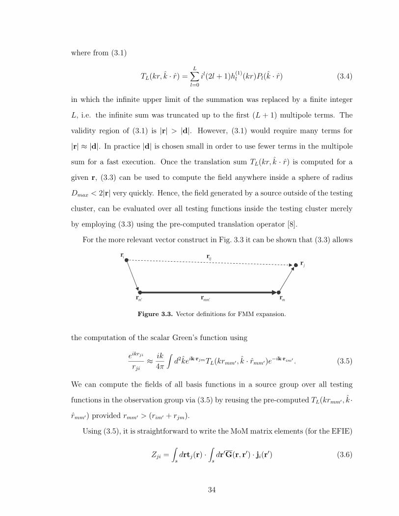
where from (3.1)

TL(kr, k · r) =L∑

l=0

il(2l + 1)h(1)l (kr)Pl(k · r) (3.4)

in which the infinite upper limit of the summation was replaced by a finite integer

L, i.e. the infinite sum was truncated up to the first (L + 1) multipole terms. The

validity region of (3.1) is |r| > |d|. However, (3.1) would require many terms for

|r| ≈ |d|. In practice |d| is chosen small in order to use fewer terms in the multipole

sum for a fast execution. Once the translation sum TL(kr, k · r) is computed for a

given r, (3.3) can be used to compute the field anywhere inside a sphere of radius

Dmax < 2|r| very quickly. Hence, the field generated by a source outside of the testing

cluster, can be evaluated over all testing functions inside the testing cluster merely

by employing (3.3) using the pre-computed translation operator [8].

For the more relevant vector construct in Fig. 3.3 it can be shown that (3.3) allows

mm′rm′r mr

jrir

ijr

Figure 3.3. Vector definitions for FMM expansion.

the computation of the scalar Green’s function using

eikrji

rji

≈ ik

4π

∫d2keik·rjmTL(krmm′ , k · rmm′)e−ik·rim′ . (3.5)

We can compute the fields of all basis functions in a source group over all testing

functions in the observation group via (3.5) by reusing the pre-computed TL(krmm′ , k ·rmm′) provided rmm′ > (rim′ + rjm).

Using (3.5), it is straightforward to write the MoM matrix elements (for the EFIE)

Zji =∫

sdrtj(r) ·

∫

sdr′G(r, r′) · ji(r′) (3.6)

34

as follows:

Zji ≈ ik

4π

∫d2kVjm(k) · TL(krmm′ , k · rmm′)V∗

im′(k), (3.7)

where

Vim′(k) =∫

Sdr′eik·rim′

[I− kk

]· ji(ri),

Vjm(k) =∫

Sdreik·rjm

[I− kk

]· tj(rj) (3.8)

and

TL(krmm′ , k · rmm′) =L∑

l=0

il(2l + 1)h(1)l (krmm′)Pl(k · ˆrmm′) . (3.9)

We remark that in FMM implementation, Zji are computed using (3.6) for nearby

testing and source basis and (3.7) is used otherwise. The fast implementation of (3.7)

between far groups of source and testing basis functions is the crux of the FMM.

In (3.7) we used the fact that[I− kk

]·[I− kk

]=

[I− kk

]to get a symmetric

equation. The terms in (3.8) are known in FMM nomenclature as the signature

functions. These are pre-computed and symmetry provides for storage savings since

we only need to compute (3.8) for the basis functions (since in Galerkin’s method,

the testing functions are chosen to be equal to the testing functions). However, this is

only true for the symmetric EFIE operator. When the MFIE operator is considered,

then

Zji = −∫

sdrtj ·

[1

2ji(r) +

∫

s−dr′n′ × ji(r

′)×∇g(r, r′)]

(3.10)

and the signatures for the basis and testing functions take the forms

Vim′(k) =∫

sdr′eik·rim′

k × [n′ × bi(ri)]

,

Vjm(k) =∫

sdreik·rjm

[I− kk

]· tj(rj). (3.11)

Here, the identity[I− kk

]·[k × a

]= k × a was used so that we can use the same

EFIE signatures of the testing functions.

The translation operator, being only dependent on the pre-chosen vector rmm′

between the points m and m′, is key to reducing the O(N2) complexity of the MoM

35

matrix-vector product in the iterative solver. By grouping the basis functions into

a pre-specified number of clusters and by reusing the translation operator to com-

pute the interactions of the basis and testing functions, the O(N2) complexity can

be reduced down to O(Nγ) where γ < 1.5. For the conventional FMM algorithm [8]

γ = 1.5, but γ can be reduced further and is close to unity for the multilevel version

of FMM. As an example, Song et al. [13] applied a nested grouping strategy along

with a flat triangular discretization and Rao-Wilton-Glisson (RWG) [2] basis func-

tions and introduced a multilevel FMM algorithm with O(N log N) computational

complexity and O(N) memory requirement. This low complexity has been achieved

by forming a multilevel grouping of the basis functions (by grouping smaller groups

in larger groups) and reusing the translation operators computed between groups at

each level, as will be outlined in the next section. We note here that there is no

restriction in the FMM algorithm on the type of surface elements and sub-sectional

basis functions used. Curvilinear surface elements and conformal basis functions as

defined in Chapter 1 are used in our specific FMM implementations. As mentioned

before, this curved surface modeling has the advantage of reducing geometry modeling

error in the solution procedure substantially. This aspect also allows us to investigate

the error performance of the FMM algorithm more accurately since the error in the

final result is dominated by the error introduced by the FMM approximation rather

than geometry modeling error, as is the case in flat triangular meshes and RWG basis

functions. Also, on each element there are 4 basis functions associated with 4 edges,

but only 2 of them are independent since adjacent elements are paired to form a basis

function. That is, curved quadrilateral elements are associated with 2 degrees of free-

dom per element, whereas flat triangles are associated with 1.5 degrees of freedom on

each element (3 basis functions are associated with the 3 edges on a single triangular

element). Quadrilateral elements also allows for better representation of the induced

surface current density on each element.

36

To take advantage of the expansion (3.7), the basis functions are grouped into

M clusters where rmm′ refers to the center-to-center distance between source group

m′ and the testing group m. Due to this a priori grouping, TL(krmm′ , k · rmm′)

is independent of the specific source/testing function pair. It only depends on the

inter-distances between the chosen groups and is pre-computed prior to the iterative

solver execution. Also, when the groups are well-separated we need a few terms in

the translation sum. Consequently, the spectral integral in (3.3) can be numerically

evaluated quickly using small number of integration points.

A most important parameter in the FMM implementation is the number of terms

kept for the evaluation of TL in (3.9). This parameter, commonly denoted as L [8],

is semi-empirically chosen as

L = kDmax + αL ln(kDmax + π) (3.12)

where Dmax is the maximum diameter of the clusters and αL is an accuracy con-

trol parameter. For αL = 5, the resulting value of L is reported to provide single

precision accuracy in evaluating TL; for αL = 10, double precision is obtained in

evaluating TL [8]. Typically, however, it has been reported [13] that setting αL = 1

gives acceptable accuracy for RCS computations. However, for geometries producing

poorly conditioned matrices (e.g. scatterers with sharp corners and/or fine detail),

any computation error in the FMM implementation is amplified by the condition

number of the system and is reflected to the final solution. When using an iterative

solver, keeping αL small will result in faster execution time but may produce large

error in the final solution. For such problems, it is a good practice to keep the FMM

approximation very accurate in order to get a correct solution at the expense of slower

solution time. As discussed in Appendix C, another remedy to this problem is to use

a low-cost preconditioner.

The spectral integral in (3.3) is discretized using L points over the θ angular

sector (Gaussian quadrature) and 2L points in the φ sector (trapezoidal rule). This

37

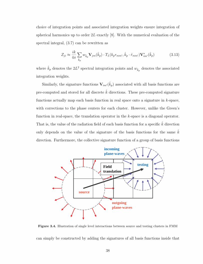
choice of integration points and associated integration weights ensure integration of

spherical harmonics up to order 2L exactly [8]. With the numerical evaluation of the

spectral integral, (3.7) can be rewritten as

Zji ≈ ik

4π

∑

kp

wkpVjm(kp) · TL(kprmm′ , kp · rmm′)V∗

im′(kp) (3.13)

where kp denotes the 2L2 spectral integration points and wkpdenotes the associated

integration weights.

Similarly, the signature functions Vim′(kp) associated with all basis functions are

pre-computed and stored for all discrete k directions. These pre-computed signature

functions actually map each basis function in real space onto a signature in k-space,

with corrections to the phase centers for each cluster. However, unlike the Green’s

function in real-space, the translation operator in the k-space is a diagonal operator.

That is, the value of the radiation field of each basis function for a specific k direction

only depends on the value of the signature of the basis functions for the same k

direction. Furthermore, the collective signature function of a group of basis functions

source

testing

outgoing plane-waves

incomingplane-waves

Fieldtranslation

Figure 3.4. Illustration of single level interactions between source and testing clusters in FMM

can simply be constructed by adding the signatures of all basis functions inside that

38

group. These two observations form the foundation of the FMM and are exploited

to obtain solution speed-up and memory reduction.

The numerical implementation of the indirect matrix-vector product computation

consists of three successive steps:

Step 1. The radiation signatures of all groups are formed by summing the

signatures of all basis functions within each group

Vm′(kp) =∑

ji∈Gm′

V∗im′(kp) (3.14)

where Gm′ denotes the set of all basis functions in the source group m′. This is called

the aggregation step.

Step 2. Provided the testing and basis groups are well seperated, group

signatures of all source groups are then translated over to the testing group via the

operation

Vm(kp) =∑

m′∈Fm′

TL(kprmm′ , kp · rmm′)Vm′(kp) (3.15)

where Fm′ is the set of source groups in the far-zone of the testing group m. Equation

(3.15) basically transforms the outgoing plane wave signatures of the source groups

onto an incoming plane wave signature on the testing group. This plane wave or spec-

tral transformation is evocative of the Fourier transform process done for uniformly

gridded testing and basis functions.

Step 3. The third and final sweep is the disaggregation used to translate the

field signatures over to the testing functions. We must note here that (3.7) is only

valid for far source and testing pairs. Hence, the interactions of basis and testing

functions in close proximity of each other must be done using the original MoM pro-

cedure. With the disaggregation step, the field over all testing functions inside the

testing domain is computed via

∑

i

Zfarji xi ≈ ik

4π

∑

kp

wkpVjm(kp) ·Vm(kp). (3.16)

39

Clearly, the smaller the groups, the less multipole terms would be required. For

example, for a maximum group size of Dmax = λ, using (3.12) with αL = 2 would

result in L+1 = 12 terms (L = kDmax+2 ln(kDmax+π) = 10.77), whereas for Dmax =

λ/2, we only need L + 1 = 8 terms. With these numbers, the spectral integral would

require 2L2 = 242 samples for the larger group size as compared to 98 samples for the

latter. However, to form smaller groups, we need to increase the number of groups and

this increases the computation of the translation operations. If N basis functions are

grouped into M groups, each group will consist of N/M basis functions. The number

of near groups for each source group will be assumed to be constant. Hence, the near-

field matrix will have O(N2/M) non-zero entries representing the near interactions

of the basis and testing functions. At the aggregation and disaggregation sweeps, the

number of flops is proportional to N × 2L2. The translation step requires M2 × 2L2

flops. Assuming that L is proportional to the maximum electrical diameter of the

groups kDmax, and that the number of basis functions in each group is proportional to

N/M , we can conclude that L2 ∝ N/M . Hence, the complexities of the aggregation

and disaggregation steps are proportional to O(N2/M), and that of the translation

step is O(NM).

Hence, the overall complexity of the FMM matrix-vector product is governed by

two competing complexities with the overall complexity given by O(N2/M + NM).

This order can be minimized by choosing M =√

N . The resulting algorithm will

then have O(N3/2) computational complexity. On top of the CPU savings of FMM,

since not all entries of the MoM matrix are needed, we will also have memory savings.

Namely, only O(N2/M) non-zero entries must be computed and stored. However, we

still need to compute and store the signature functions and the translation operator.

The storage requirement of the signature functions is O(2L2N) = O(N2/M) and that

of the translation operator is O(2L2M2) = O(NM). The sum of these requirements is

also minimized for M =√

N and the total storage complexity of the solution method

40

is reduced down to O(N3/2).

The above CPU estimates are asymptotic in the sense that they represent values

which are approached for very large N . The actual efficiency of the implementation

depends on the choices of various parameters. These choices control the constant

in front of the asymptotic behavior of the CPU requirements. However, choices

of the FMM parameters for faster implementation inevitably lead to less accurate

answers. Clearly, keeping L as small as possible reduces the CPU time but not the

order. That is, if the CPU time is given by CN3/2 for the matrix vector product

computation (C = constant), lowering L implies smaller value for the constant.

Lower C values imply that the CPU time crossover point between standard MoM

and FMM implementations occurs for lower values of N .

Another key area that determines FMM efficiency is that of element grouping.

Here, for the single level FMM implementation, we used the k-means algorithm [50]

to form the clusters. This algorithm aims to minimize a defined error function for the

purpose of achieving a fairly uniform set of groups. The specific error function used by

the k-means algorithm minimizes the sum of the distances between the cluster centers

and the centers of the basis functions in each cluster. If the resulting clustering is

not uniform, the FMM implementation will be inefficient due to the presence of very

large or very small clusters. This affects the computation time due to the spectral

integral since the number of terms used in the translation sum will depend on the

size of the largest cluster. Although the k-means algorithm provides a fairly uniform

grouping, it is always unstructured as shown in Fig. 3.5. As will be discussed in

the multilevel implementation of the FMM, a structured grouping, such as one that

consists of cubic groups having translational symmetry, can provide further savings

in the storage of the translation operator since some of the translation operators will

be identical due to translational symmetry.

In the FMM implementation, the approximation (3.7) is only used for computing

41

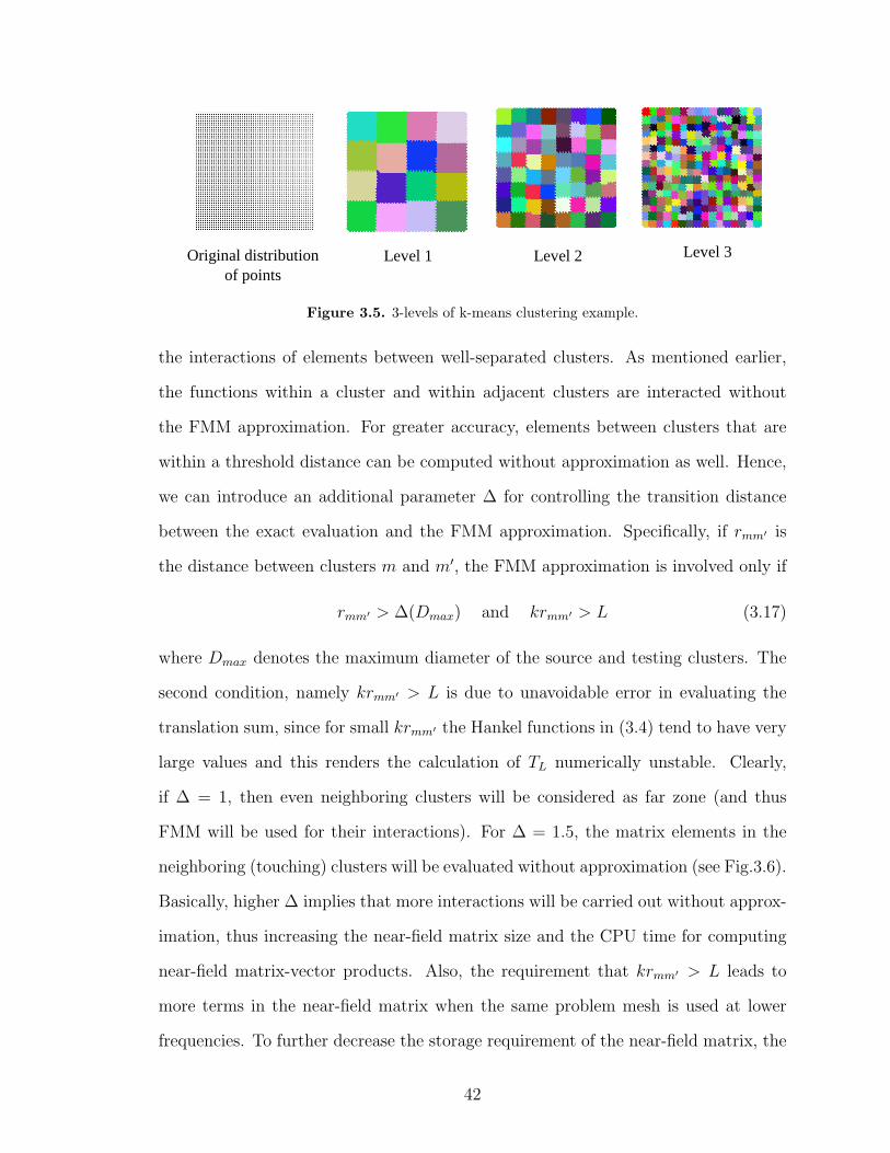
Level 3Level 2Level 1Original distribution of points

Figure 3.5. 3-levels of k-means clustering example.

the interactions of elements between well-separated clusters. As mentioned earlier,

the functions within a cluster and within adjacent clusters are interacted without

the FMM approximation. For greater accuracy, elements between clusters that are

within a threshold distance can be computed without approximation as well. Hence,

we can introduce an additional parameter ∆ for controlling the transition distance

between the exact evaluation and the FMM approximation. Specifically, if rmm′ is

the distance between clusters m and m′, the FMM approximation is involved only if

rmm′ > ∆(Dmax) and krmm′ > L (3.17)

where Dmax denotes the maximum diameter of the source and testing clusters. The

second condition, namely krmm′ > L is due to unavoidable error in evaluating the

translation sum, since for small krmm′ the Hankel functions in (3.4) tend to have very

large values and this renders the calculation of TL numerically unstable. Clearly,

if ∆ = 1, then even neighboring clusters will be considered as far zone (and thus

FMM will be used for their interactions). For ∆ = 1.5, the matrix elements in the

neighboring (touching) clusters will be evaluated without approximation (see Fig.3.6).

Basically, higher ∆ implies that more interactions will be carried out without approx-

imation, thus increasing the near-field matrix size and the CPU time for computing

near-field matrix-vector products. Also, the requirement that krmm′ > L leads to

more terms in the near-field matrix when the same problem mesh is used at lower

frequencies. To further decrease the storage requirement of the near-field matrix, the

42

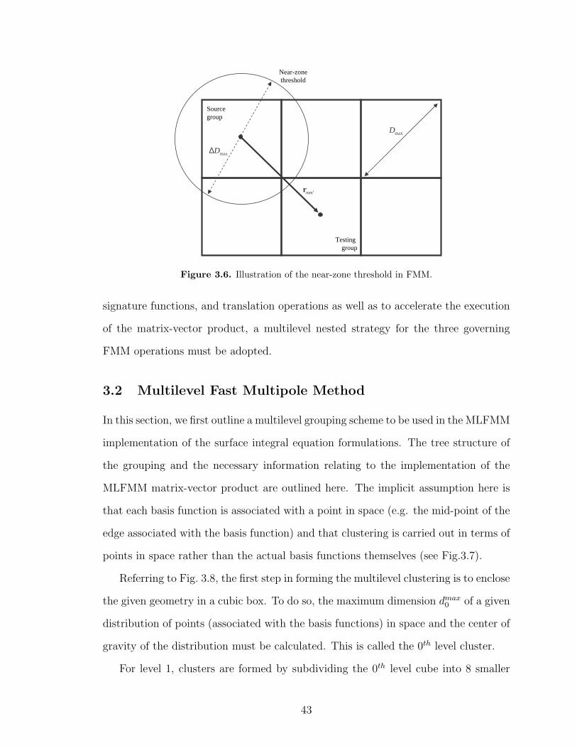
maxD

maxD∆

mm′r

Near-zonethreshold

Source group

Testing group

Figure 3.6. Illustration of the near-zone threshold in FMM.

signature functions, and translation operations as well as to accelerate the execution

of the matrix-vector product, a multilevel nested strategy for the three governing

FMM operations must be adopted.

3.2 Multilevel Fast Multipole Method

In this section, we first outline a multilevel grouping scheme to be used in the MLFMM

implementation of the surface integral equation formulations. The tree structure of

the grouping and the necessary information relating to the implementation of the

MLFMM matrix-vector product are outlined here. The implicit assumption here is

that each basis function is associated with a point in space (e.g. the mid-point of the

edge associated with the basis function) and that clustering is carried out in terms of

points in space rather than the actual basis functions themselves (see Fig.3.7).

Referring to Fig. 3.8, the first step in forming the multilevel clustering is to enclose

the given geometry in a cubic box. To do so, the maximum dimension dmax0 of a given

distribution of points (associated with the basis functions) in space and the center of

gravity of the distribution must be calculated. This is called the 0th level cluster.

For level 1, clusters are formed by subdividing the 0th level cube into 8 smaller

43

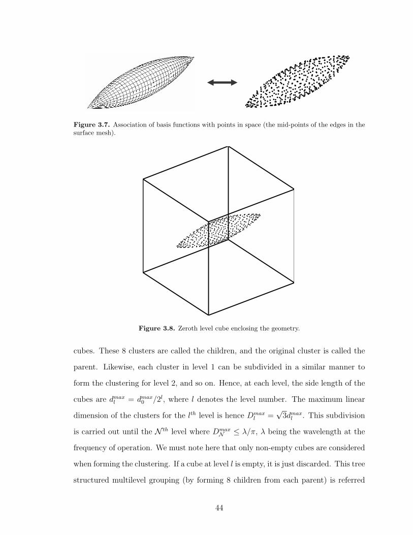
Figure 3.7. Association of basis functions with points in space (the mid-points of the edges in thesurface mesh).

Figure 3.8. Zeroth level cube enclosing the geometry.

cubes. These 8 clusters are called the children, and the original cluster is called the

parent. Likewise, each cluster in level 1 can be subdivided in a similar manner to

form the clustering for level 2, and so on. Hence, at each level, the side length of the

cubes are dmaxl = dmax

0 /2l, where l denotes the level number. The maximum linear

dimension of the clusters for the lth level is hence Dmaxl =

√3dmax

l . This subdivision

is carried out until the N th level where DmaxN ≤ λ/π, λ being the wavelength at the

frequency of operation. We must note here that only non-empty cubes are considered

when forming the clustering. If a cube at level l is empty, it is just discarded. This tree

structured multilevel grouping (by forming 8 children from each parent) is referred

44

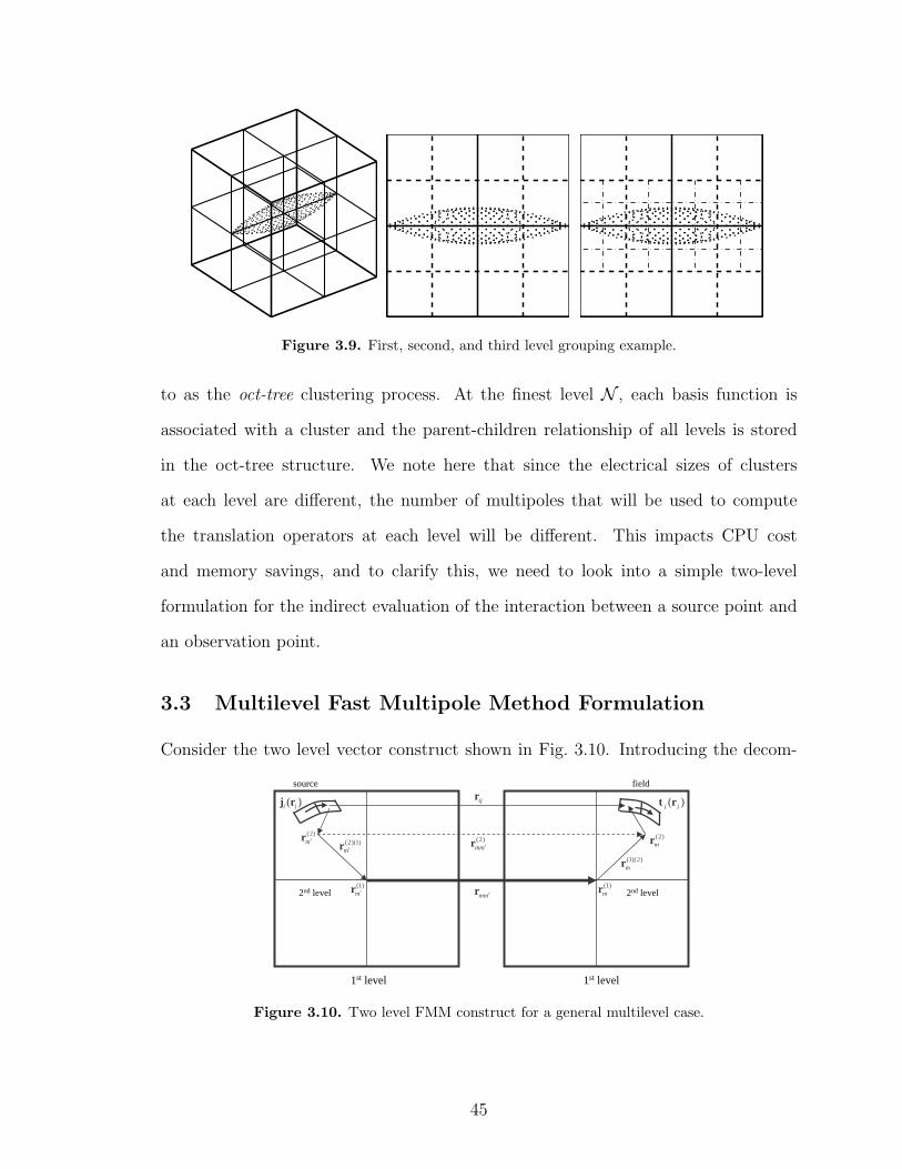
Figure 3.9. First, second, and third level grouping example.

to as the oct-tree clustering process. At the finest level N , each basis function is

associated with a cluster and the parent-children relationship of all levels is stored

in the oct-tree structure. We note here that since the electrical sizes of clusters

at each level are different, the number of multipoles that will be used to compute

the translation operators at each level will be different. This impacts CPU cost

and memory savings, and to clarify this, we need to look into a simple two-level

formulation for the indirect evaluation of the interaction between a source point and

an observation point.

3.3 Multilevel Fast Multipole Method Formulation

Consider the two level vector construct shown in Fig. 3.10. Introducing the decom-

source field

1st level

2nd level 2nd levelmm′r

(2)(1)m′r

(1)(2)mr

(2)mm′r

ijr( )i ij r ( )j jt r

1st level

(1)m′r (1)

mr

(2)m′r (2)

mr

Figure 3.10. Two level FMM construct for a general multilevel case.

45

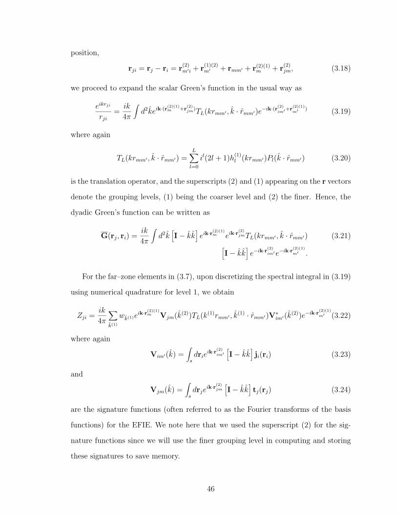
position,

rji = rj − ri = r(2)m′i + r

(1)(2)m′ + rmm′ + r(2)(1)

m + r(2)jm, (3.18)

we proceed to expand the scalar Green’s function in the usual way as

eikrji

rji

=ik

4π

∫d2keik·(r(2)(1)

m +r(2)jm)TL(krmm′ , k · rmm′)e−ik·(r(2)

im′+r(2)(1)

m′ ) (3.19)

where again

TL(krmm′ , k · rmm′) =L∑

l=0

il(2l + 1)h(1)l (krmm′)Pl(k · rmm′) (3.20)

is the translation operator, and the superscripts (2) and (1) appearing on the r vectors

denote the grouping levels, (1) being the coarser level and (2) the finer. Hence, the

dyadic Green’s function can be written as

G(rj, ri) =ik

4π

∫d2k

[I− kk

]eik·r(2)(1)

m eik·r(2)jmTL(krmm′ , k · rmm′) (3.21)

[I− kk

]e−ik·r(2)

im′e−ik·r(2)(1)

m′ .

For the far–zone elements in (3.7), upon discretizing the spectral integral in (3.19)

using numerical quadrature for level 1, we obtain

Zji =ik

4π

∑

k(1)

wk(1)eik·r(2)(1)

m Vjm(k(2))TL(k(1)rmm′ , k(1) · rmm′)V∗im′(k(2))e−ik·r(2)(1)

m′ (3.22)

where again

Vim′(k) =∫

sdrie

ik·r(2)

im′[I− kk

]ji(ri) (3.23)

and

Vjm(k) =∫

sdrje

ik·r(2)jm

[I− kk

]tj(rj) (3.24)

are the signature functions (often referred to as the Fourier transforms of the basis

functions) for the EFIE. We note here that we used the superscript (2) for the sig-

nature functions since we will use the finer grouping level in computing and storing

these signatures to save memory.

46

It is observed in (3.22) that the discrete values of the signature functions Vim′(k(2))

and Vjm(k(2)) are for the k-space discretization at level 2. The computation of (3.22)

requires their k-space values at level 1 since the translation operator is generated for

the sampling at level 1. We can use interpolation to generate the required k-space

samples. Referring to Fig. 3.11 for a smooth function f(θ), given the samples f(θi)

( )f θ

θ

Polynomial fit points

Lagrangeinterpolators

Original samples: θi

Samples to beinterpolated: θk

kθ1W ( )i θ+

W ( )i θ

iθ

Figure 3.11. Illustration of interpolation matrices in FMM.

at θi, i = 1, ..., L(2), we can generate a different sampling at θk, k = 1, ..., L(1) via

interpolation. From the known values of f(θi) we can form an approximation to f(θ)

via

f(θ) =∑

i

Wi(θ)f(θi) (3.25)

where Wi(θ) are the interpolators which are simple quadratics for the example shown

in Fig. 3.11. To generate the new sampling, (3.25) is evaluated at θk, i.e.

f(θk) =∑

i

Wi(θk)f(θi), k = 1, ..., L(2). (3.26)

The above equation can be cast in a matrix form as fk = Wkifi, where fi = f(θi) and

Wki = Wi(θk). For a general case, the interpolation matrix Wki is a full matrix.

However, in this case, the overall performance of the MLFMM is dictated by the high

47

complexity of the interpolation operation. Hence, a sparse interpolation method is

necessary not to exacerbate MLFMM performance. One possible method is to use

a fixed order polynomial interpolation scheme as shown in Fig. 3.11. For this case,

the generated interpolation matrix is sparse since only a few interpolators around the

new sample θk are included in the computation of f(θk).

For the signature functions, same method can be employed on the unit sphere (i.e.

on k space) via

Vim′(k(1)) = WVim′(k(2))

= W(1),(2)Vim′(k(2)) (3.27)

where W(1),(2) refers to the interpolation coefficients between levels 1 and 2. We also

note the property

Vim′(k(2)) = WT(1),(2)Vim′(k(1)) (3.28)

where the superscript T implies matrix transposition. This interpolation strategy

enables the generation of signatures of parent clusters using the collective signatures

of its children. We must note here that the interpolated signatures of the children

must also be phase-corrected through a simple phase-shifting operation as given in

(3.22).

The matrix-vector product for this two-level grouping can be carried out as follows.

The aggregations are done for the source clusters at the finer level 2 for each k(2)

direction. The k-space sampling of the aggregated field signatures of the source

clusters are then interpolated to compute the signatures on the required k-space

samples at level 1 using (3.27). The phase centers of the aggregated field signatures

of the source clusters are then shifted to the center of the parent source clusters

at the coarser level 1 by simply multiplying with e−ik·r(2)(1)

m′ as in (3.22). The same

procedure is applied to all non-empty children corresponding to source clusters at

level 1. After translating the signature onto the field cluster at this coarse level, the

same operations are carried out in reverse order to compute the final matrix-vector

48

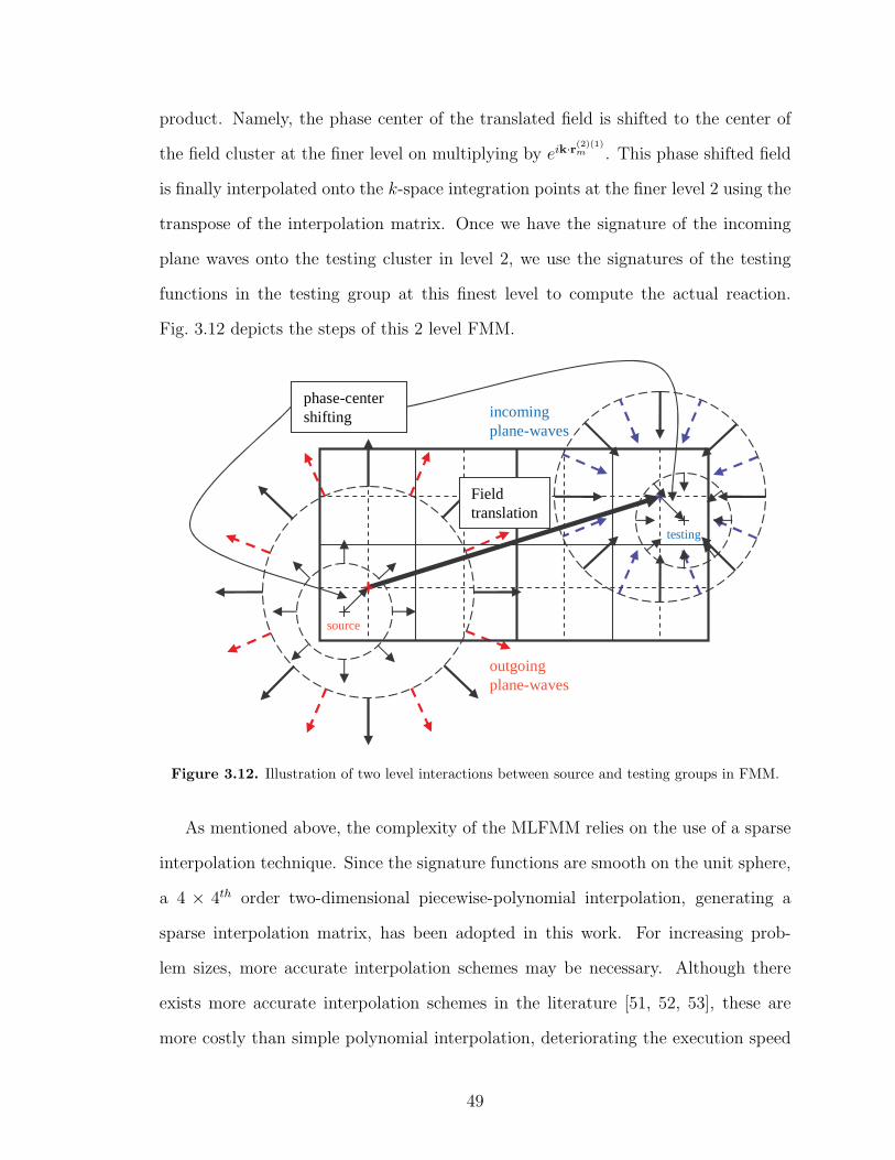
product. Namely, the phase center of the translated field is shifted to the center of

the field cluster at the finer level on multiplying by eik·r(2)(1)m . This phase shifted field

is finally interpolated onto the k-space integration points at the finer level 2 using the

transpose of the interpolation matrix. Once we have the signature of the incoming

plane waves onto the testing cluster in level 2, we use the signatures of the testing

functions in the testing group at this finest level to compute the actual reaction.

Fig. 3.12 depicts the steps of this 2 level FMM.

source

testing

outgoing plane-waves

incoming plane-waves

Fieldtranslation

phase-centershifting

Figure 3.12. Illustration of two level interactions between source and testing groups in FMM.

As mentioned above, the complexity of the MLFMM relies on the use of a sparse

interpolation technique. Since the signature functions are smooth on the unit sphere,

a 4 × 4th order two-dimensional piecewise-polynomial interpolation, generating a

sparse interpolation matrix, has been adopted in this work. For increasing prob-

lem sizes, more accurate interpolation schemes may be necessary. Although there

exists more accurate interpolation schemes in the literature [51, 52, 53], these are

more costly than simple polynomial interpolation, deteriorating the execution speed

49

of the matrix-vector product.

It is necessary that the multilevel grouping algorithm provide the neighborhood

information of all clusters at all levels. When constructing the far-zone clusters for

a cluster i at level (l + 1), the condition is that the parents (at level (l)) of clusters

i and j at level (l + 1) be in the near-zone of each other (see Fig. 3.13). Otherwise,

the interactions of clusters i and j are computed through translations at the coarser

level (l).

Sample cluster

Near clusters

Far clusters

i level clusteringth

(i-1) level clusteringth

Figure 3.13. 2-dimensional multilevel clustering example.

In the most general multilevel form, there are five steps in the MLFMM:

Step 1. All the collective signatures of all source functions in the finest level are

computed using the individual signatures of the basis functions.

Step 2. For all coarser levels, the collective signatures are calculated through inter-

polation and shifting using the signatures of the children.

Step 3. For each level (l) these signatures are translated onto far clusters such that

their parents are in the near-zone of each other at level (l + 1).

Step 4. The translated incoming signatures are shifted and interpolated onto the

children at the finer levels.

Step 5. At the finest level, the interactions are computed using the signatures of the

50

testing functions and the incoming plane wave decompositions.

This multilevel tree-structure provides O(N log N) CPU and memory complexity.

Furthermore, due to the translational symmetry in the grouping, significant memory

saving is achieved in the storage of the translation operator. This low O(N log N)

complexity enables the solution of significantly larger problems on low-cost personal

computer platforms. This is demonstrated in the next section. Nevertheless, as

the target becomes larger, one must resort to supercomputers. The challenges in

implementing the MLFMM on distributed memory computers are addressed in Ap-

pendix D.

3.4 Examples and Validations

Below, we present validations and complexity evaluations of the implemented ML-

FMM solver for electromagnetic scattering and radiation problems involving elec-

trically large arbitrarily shaped targets in free space. For the presented data, the

MLFMM strategy has been implemented using curved biquadratic surface elements

and conformal rooftop basis functions as described above. However, the previous

development of the MLFMM applies to any element shape and basis function.

Our first example is a radiation problem. A Hertzian dipole is placed above a PEC

sphere. This problem has a closed form solution and hence constitutes a benchmark.

The problem was solved at three different frequencies using the same surface mesh of

the sphere. This also serves for the evaluation of using curvilinear elements aiming at

reducing the sampling requirements. Fig. 3.14 depicts the induced surface currents

for the simulation frequencies. The creeping wave effects in the shadow region of

the sphere are clearly resolved in these current amplitude plots. A more important

observable in case of radiation scenarios is the radiation pattern. Fig. 3.15 depicts

the normalized patterns at the corresponding frequencies along with the analytical

Mie series solution [27].

51

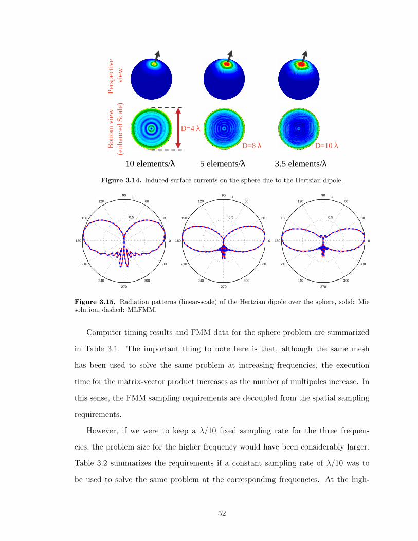
10 elements/λ 5 elements/λ 3.5 elements/λ

D=4 λ

D=8 λ D=10 λBot

tom

vie

w(e

nhan

ced

Sca

le)

Per

spec

tive

vi

ew

Figure 3.14. Induced surface currents on the sphere due to the Hertzian dipole.

0.5

1

30

210

60

240

90

270

120

300

150

330

180 0

0.5

1

30

210

60

240

90

270

120

300

150

330

180 0

0.5

1

30

210

60

240

90

270

120

300

150

330

180 0

Figure 3.15. Radiation patterns (linear-scale) of the Hertzian dipole over the sphere, solid: Miesolution, dashed: MLFMM.

Computer timing results and FMM data for the sphere problem are summarized

in Table 3.1. The important thing to note here is that, although the same mesh

has been used to solve the same problem at increasing frequencies, the execution

time for the matrix-vector product increases as the number of multipoles increase. In

this sense, the FMM sampling requirements are decoupled from the spatial sampling

requirements.

However, if we were to keep a λ/10 fixed sampling rate for the three frequen-

cies, the problem size for the higher frequency would have been considerably larger.

Table 3.2 summarizes the requirements if a constant sampling rate of λ/10 was to

be used to solve the same problem at the corresponding frequencies. At the high-

52

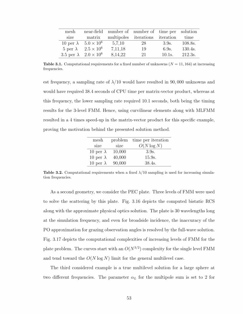
mesh near-field number of number of time per solutionsize matrix multipoles iterations iteration time

10 per λ 5.0× 106 5,7,10 28 3.9s. 108.8s.5 per λ 2.5× 106 7,11,18 19 6.9s. 130.4s.

3.5 per λ 2.0× 106 8,14,22 21 10.1s. 212.3s.

Table 3.1. Computational requirements for a fixed number of unknowns (N = 11, 164) at increasingfrequencies.

est frequency, a sampling rate of λ/10 would have resulted in 90, 000 unknowns and

would have required 38.4 seconds of CPU time per matrix-vector product, whereas at

this frequency, the lower sampling rate required 10.1 seconds, both being the timing

results for the 3-level FMM. Hence, using curvilinear elements along with MLFMM

resulted in a 4 times speed-up in the matrix-vector product for this specific example,

proving the motivation behind the presented solution method.

mesh problem time per iterationsize size O(N log N)

10 per λ 10,000 3.9s.10 per λ 40,000 15.9s.10 per λ 90,000 38.4s.

Table 3.2. Computational requirements when a fixed λ/10 sampling is used for increasing simula-tion frequencies.

As a second geometry, we consider the PEC plate. Three levels of FMM were used

to solve the scattering by this plate. Fig. 3.16 depicts the computed bistatic RCS

along with the approximate physical optics solution. The plate is 30 wavelengths long

at the simulation frequency, and even for broadside incidence, the inaccuracy of the

PO approximation for grazing observation angles is resolved by the full-wave solution.

Fig. 3.17 depicts the computational complexities of increasing levels of FMM for the

plate problem. The curves start with an O(N3/2) complexity for the single level FMM

and tend toward the O(N log N) limit for the general multilevel case.

The third considered example is a true multilevel solution for a large sphere at

two different frequencies. The parameter αL for the multipole sum is set to 2 for

53

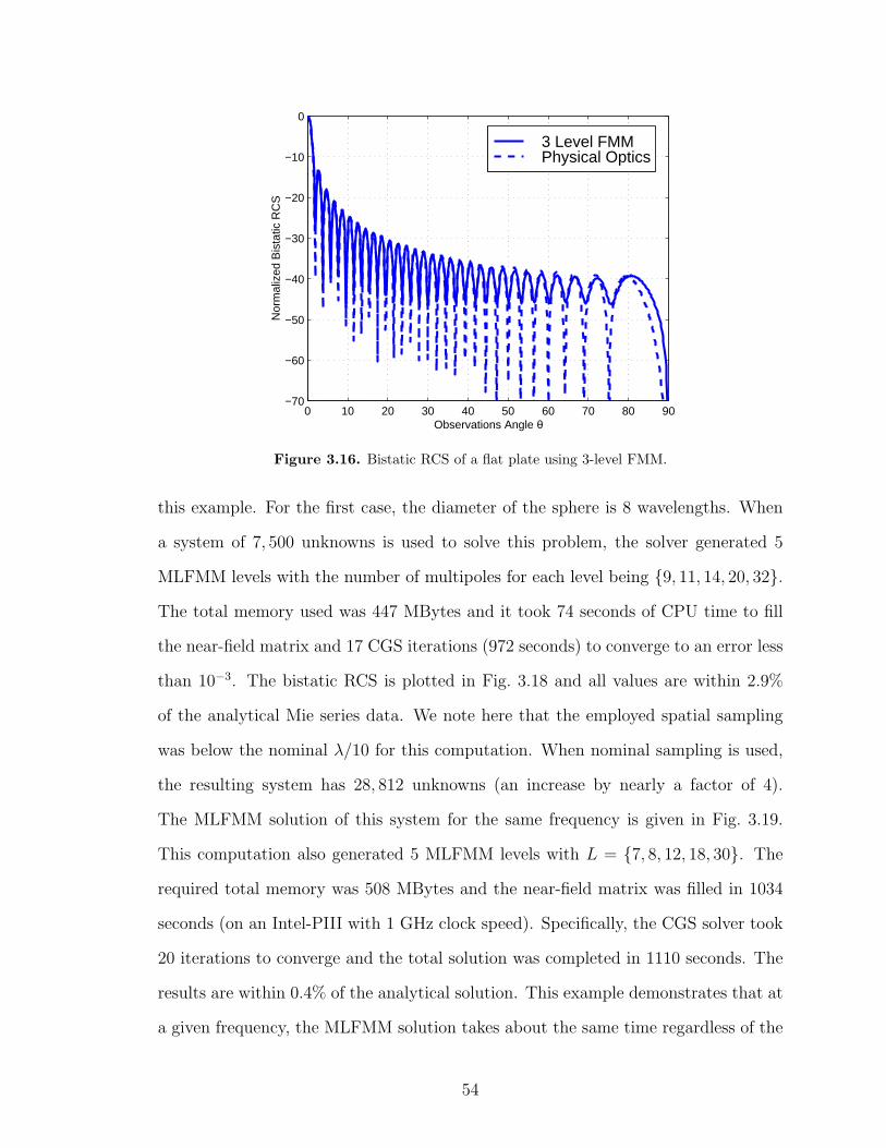
0 10 20 30 40 50 60 70 80 90−70

−60

−50

−40

−30

−20

−10

0

Observations Angle θ

Nor

mal

ized

Bis

tatic

RC

S

3 Level FMMPhysical Optics

Figure 3.16. Bistatic RCS of a flat plate using 3-level FMM.

this example. For the first case, the diameter of the sphere is 8 wavelengths. When

a system of 7, 500 unknowns is used to solve this problem, the solver generated 5

MLFMM levels with the number of multipoles for each level being 9, 11, 14, 20, 32.The total memory used was 447 MBytes and it took 74 seconds of CPU time to fill

the near-field matrix and 17 CGS iterations (972 seconds) to converge to an error less

than 10−3. The bistatic RCS is plotted in Fig. 3.18 and all values are within 2.9%

of the analytical Mie series data. We note here that the employed spatial sampling

was below the nominal λ/10 for this computation. When nominal sampling is used,

the resulting system has 28, 812 unknowns (an increase by nearly a factor of 4).

The MLFMM solution of this system for the same frequency is given in Fig. 3.19.

This computation also generated 5 MLFMM levels with L = 7, 8, 12, 18, 30. The

required total memory was 508 MBytes and the near-field matrix was filled in 1034

seconds (on an Intel-PIII with 1 GHz clock speed). Specifically, the CGS solver took

20 iterations to converge and the total solution was completed in 1110 seconds. The

results are within 0.4% of the analytical solution. This example demonstrates that at

a given frequency, the MLFMM solution takes about the same time regardless of the

54

102

103

104

105

106

10−3

10−2

10−1

100

101

102

103

104

105

Number of Unknowns

CP

U ti

me

per

itera

tion

MoMFMM−1FMM−2FMM−3Measured

Figure 3.17. Complexities of various levels of the FMM.

spatial sampling, and this is due to the frequency domain nature of the formulation.

As will be discussed later, this property proves to be very useful in solving VIEs

involving high contrast material parameters where the sampling rate is determined

by the wavelength inside the inhomogeneity and is therefore much higher as compared

to that on PEC surfaces. However, since the k-space sampling is based on the Green’s

function, the number of samples is independent of the specific material parameters

present in the problem.

When the 28, 812 unknown mesh is used to solve the problem at twice the fre-

quency, i.e. for a 16λ diameter sphere, the solver generated 6 MLFMM levels with

L = 9, 11, 14, 20, 32, 55. The solution required 1.1 GBytes of memory and the near-

field matrix was filled in 933 seconds. The CGS solver converged in 18 iterations

taking a total time of 4185 seconds. The actual RCS is shown in Fig. 3.20 and is

within 2.6% of the reference Mie series solution. When we used a nominally dis-

cretized mesh, 110, 190 unknowns are needed and the corresponding solution is given

in Fig. 3.21. The computed bistatic RCS is now within 0.6% of the reference solution

for this case. Were we to use traditional MoM solution procedures (with Gaussian

55

0 45 95 135 1800

10

20

30

40

50

60

Observation angle θ (degrees)

Bis

tatic

RC

S (

dB/λ

2 )

CFIE(α=0.5) Solution for Isoparametric Mesh

MieMoM

Figure 3.18. Bistatic RCS of an 8λ diameter PEC sphere using 7, 500 unknowns.

elimination or LU decomposition) 97.1 GBytes would have been required and this is

well beyond the storage capacity even for supercomputing facilities.

Nevertheless, even with the MLFMM, when the storage exceeds 4 Gbytes, we

must then resort to using multiprocessor supercomputing resources. Porting of the

MLFMM algorithm on distributed memory supercomputers requires a carefully bal-

anced distribution of the problem among the individual processors and minimization

of inter-processor communication. A brief discussion on the challenges of distributed

memory implementation of the MLFMM using the Message Passing Interface (MPI)

programming paradigm is given in Appendix D.

56

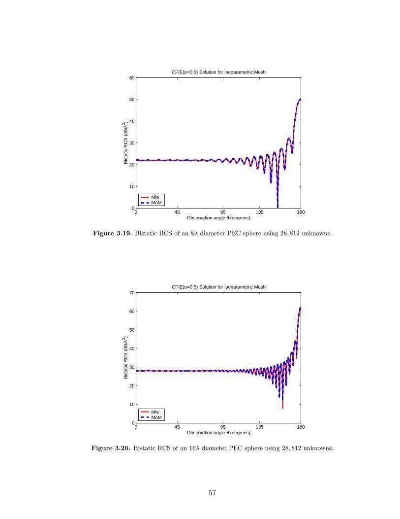
0 45 95 135 1800

10

20

30

40

50

60

Observation angle θ (degrees)

Bis

tatic

RC

S (

dB/λ

2 )

CFIE(α=0.5) Solution for Isoparametric Mesh

MieMoM

Figure 3.19. Bistatic RCS of an 8λ diameter PEC sphere using 28, 812 unknowns.

0 45 95 135 1800

10

20

30

40

50

60

70

Observation angle θ (degrees)

Bis

tatic

RC

S (

dB/λ

2 )

CFIE(α=0.5) Solution for Isoparametric Mesh

MieMoM

Figure 3.20. Bistatic RCS of an 16λ diameter PEC sphere using 28, 812 unknowns.

57

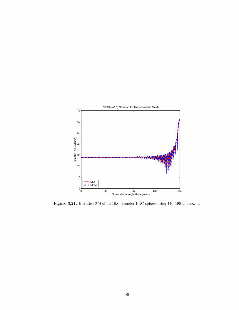
0 45 95 135 1800

10

20

30

40

50

60

70

Observation angle θ (degrees)

Bis

tatic

RC

S (

dB/λ

2 )

CFIE(α=0.5) Solution for Isoparametric Mesh

MieMoM

Figure 3.21. Bistatic RCS of an 16λ diameter PEC sphere using 110, 190 unknowns.

58

CHAPTER 4

Hybrid Finite Element-Boundary Integral Method

for Volumetric Problems

Electromagnetic scattering by inhomogeneous structures is of great interest in

evaluating the overall scattering by modern composite vehicles. The same mathe-

matical formulations are also suited for antennas, high frequency microwave circuits,

electromagnetic coupling and interference, and inverse scattering applications. Thus,

much interest exists in developing efficient formulations and numerical solutions in

modeling electrically large volumetric problems having arbitrary permittivity (ε) and

permeability (µ).

During the 1990s, treatment of inhomogeneous scatterers focused on finite ele-

ment (FE) methods [18] and their hybrid finite element-boundary integral (FE-BI)

counterparts [18, 19, 54, 55]. The FE methods with approximate mesh termina-

tion schemes, such as absorbing boundary conditions, artificial absorbers, or per-

fectly matched layers, were found attractive because of their geometrical and mate-

rial adaptability coupled with their low memory requirements. The introduction of

fast integral methods [44, 56] prompted renewed interest in the solution of FE-BI

formulations for large-scale simulations.

In this chapter, we consider the hybrid FE-BI formulations for scattering by pene-

trable structures. Again using curvilinear elements as in [19], we present the MLFMM

implementation for electrically large inhomogeneous problems. For completeness,

here we describe the geometry modeling by curvilinear hexahedral elements and con-

formal electric field basis functions as well as the mathematical tools used to develop

59

the formulations in parametric coordinates. This information will also be used in the

next chapter when we consider the alternative VIE methods.

4.1 FE-BI Formulation

FE [18, 55, 57] and FE-BI methods have been among the workhorse techniques for

frequency domain simulations over the past ten years. Here, we present the FE-BI

from a general viewpoint as applied to non-planar structures [19]. However, our main

contribution is the introduction of the MLFMM within the FE-BI context.

In formulating the FE-BI, we begin with the functional for the electric field in the

solution domain v (see Fig. 4.1) given by

F (E) =1

2

∫

vdr

[(∇× E) · µ−1

r · (∇× E)− k20E · εr · E

]− ik0η0

∫

sdrn ·(E×H) (4.1)

where µr and εr are the tensor constitutive parameters of the inhomogeneous medium,

k0 and η0 are the wavenumber and characteristic impedance in free-space, and the

boundary s encloses the volume v with n pointing outward from v as shown in Fig. 4.1.

For a unique solution, it is necessary to relate E and H on the bounding surface s to

ε (r), µ (r)0 0

vε(r), µ(r)

s=∂v

v0 s =∂v0 0

xy

z

E (r)inc

k(r)H (r)inc

n

Figure 4.1. FE-BI solution domain.

obtain an equation in terms of E only. This is done by introducing the Stratton-Chu

60

integral equations [22]. The electric field integral equation (EFIE) is given by

η0Θn×H − ΩE× n = Einc, (4.2)

whereas the magnetic field integral equation (MFIE) has the form

η0Ωn×H+ ΘE× n = η0Hinc, (4.3)

in which the integral operators Θ· and Ω· are defined as

Θ(X) = −ik0

∫

sdr′G(r, r′) ·X(r′)

= −ik0

[∫

sdr′g(r, r′)X(r′) +

1

k20

∫

sdr′∇g(r, r′)∇′ ·X(r′)

](4.4)

Ω(X) = TY(r) +∫

s−dr′X(r′)×∇g(r, r′)

with T = 1− β/4π (β = 2π for a smooth surface), n denoting the unit normal to the

bounding surface, and the relation X = n×Y. Typically, a combination of the two,

referred to as the CFIE, is employed to avoid internal resonance difficulties and poor

conditioning.

The electric field is solved from (4.1) by setting ∂F (E)/∂E = 0. Discretizing

the resulting equations using the appropriate expansion [19] (assuming no internal

excitations inside v) results in the system

Evv Evs 0

Esv Ess B

0 P Q

Ev

Es

Hs

=

0

0

b

(4.5)

where the bold symbols Evv, Evs, Esv, Ess, B, P, and Q represent sub-matrices.

61

Specifically, the elements of the sub-matrices in (4.5) are given as

Eji =∫

vdr∇× ej · µ−1

r · ∇ × ei +∫

vdrej · εr · ei

Bji = ik0η0

∫

sdrej · (n× hsi)

Pji =∫

sdr(n× hsj) · [−αΩei × n+ (1− α)Θei × n]

Qji = η0

∫

sdr(n× hsj) · [αΘn× hsi+ (1− α)Ωn× hsi]

bj = α∫

sdr(n× hsj) · Einc + (1− α)η0

∫

sdr(n× hsj) ·Hinc (4.6)

where ei and ej denote the basis and testing functions for the volume electric field

intensities, respectively. Also, the surface magnetic field intensity is expanded using

the basis functions hs and α is the CFIE scale factor chosen from zero to unity.

However, we can use the definitions J = n×H and M = E× n and define expansions

of these surface quantities in the integral operators. With J =∑

i hsiji and M =

∑i esimi, the matrix entries for the integral operators in (4.6) can be rewritten in a

more compact form (for CFIE) as

Pji =∫

sdrjj · [−αΩmi+ (1− α)Θmi]

Qji = η0

∫

sdrjj · [αΘji+ (1− α)Ωji]

bj = α∫

sdrjj · Einc + (1− α)η0

∫

sdrjj ·Hinc. (4.7)

We note here that the basis functions used in expanding the surface unknowns are

identical to those presented in Chapter 2. Specifically, for mi this is a direct con-

sequence of the definition mi = ei × n. The electric current unknowns which are

independent in the formulation are defined using the same conformal basis functions.

For a general inhomogeneous structure consisting of material and conducting com-

ponents, the resulting system in (4.5) is highly heterogeneous, consisting of a sparse

FE part ([E] and [B] sub-matrices) and a full integral equation part ([P ] and [Q] sub-

matrices). This highly heterogeneous FE-BI system may result in a poorly convergent

iterative solution, especially for large scale systems. To obtain an improved matrix

62

condition for (4.5), we can test the MFIE of (4.3) with n × jj [45, 58], rather than

simply testing it with jj as done in (4.7). The aim is to generate a strong diagonal

contribution in [Q] and a weak diagonal contribution in [P ]. Doing so, the resulting

matrix entries take the form

Pji = −α∫

sdrjj · Ωmi+ (1− α)

∫

sdr(n× jj) ·Θmi

Qji = αη0

∫

sdrjj ·Θji+ (1− α)

∫

sdr(n× jj) · Ωji

bj = α∫

sdrjj · Einc + (1− α)η0

∫

sdr(n× jj) ·Hinc, (4.8)

and this should be compared to (4.7).

Since the application of fast methods (such as the MLFMM) implies use of it-

erative solvers, a poor convergence behavior implies serious difficulties in terms of

total solution time, especially for multi-spectral simulations. Preconditioning meth-

ods may therefore be necessary for certain problems to achieve convergence. Clearly,

it is important to use preconditioners which can be implemented in favorable CPU

times. Among them, the block-diagonal [39] and the ILU [40] preconditioners have

been found quite effective. In modeling layered geometries, substantial improvement

in matrix condition can be achieved by choosing hexahedral elements rather than

tetrahedra. Curvilinear elements also allow for geometrical modeling fidelity and have

been shown effective for antenna arrays [59] as well as scattering applications [19, 31].

When dealing with large antenna arrays, certain advantages associated with the re-

peatability of each array element can be exploited. Details of such a decomposition

method can be found in [59].

We outlined the MLFMM in Chapter 3 for perfectly conducting targets. However,

since the integral operators in (4.8) are identical to those used in Chapter 2, the

outlined MLFMM implementation can be extended to the FE-BI method and to VIE

formulations by merely incorporating the signature functions into their respective

algorithms. Specifically, for the FE-BI method, since the same basis functions are

63

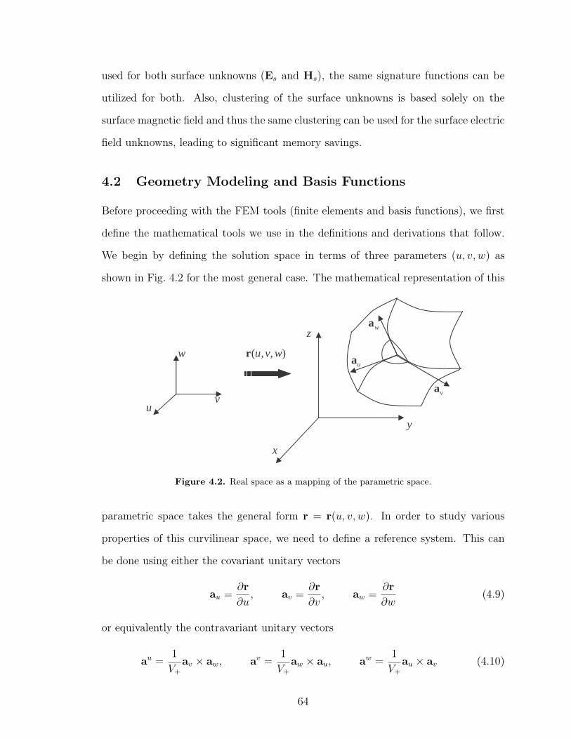
used for both surface unknowns (Es and Hs), the same signature functions can be

utilized for both. Also, clustering of the surface unknowns is based solely on the

surface magnetic field and thus the same clustering can be used for the surface electric

field unknowns, leading to significant memory savings.

4.2 Geometry Modeling and Basis Functions

Before proceeding with the FEM tools (finite elements and basis functions), we first

define the mathematical tools we use in the definitions and derivations that follow.

We begin by defining the solution space in terms of three parameters (u, v, w) as

shown in Fig. 4.2 for the most general case. The mathematical representation of this

uv

w

x

y

z

ua

va

wa

( , , )u v wr

Figure 4.2. Real space as a mapping of the parametric space.

parametric space takes the general form r = r(u, v, w). In order to study various

properties of this curvilinear space, we need to define a reference system. This can

be done using either the covariant unitary vectors

au =∂r

∂u, av =

∂r

∂v, aw =

∂r

∂w(4.9)

or equivalently the contravariant unitary vectors

au =1

V+

av × aw, av =1

V+

aw × au, aw =1

V+

au × av (4.10)

64

where V+ = au · (av × aw) is used for normalization. We must note the property that

ai · aj = δij (i, j = u, v, w) where δij is the Kronecker delta function.

The Jacobian of the parametric transformation r(u, v, w) is given by

[J ] =

∂x∂u

∂y∂u

∂z∂u

∂x∂v

∂y∂v

∂z∂v

∂x∂w

∂y∂w

∂z∂w

(4.11)

and the metric tensor is

[G] =

guu guv guw

gvu gvv gvw

gwu gwv gww

(4.12)

with gij = ai · aj. This metric completely characterizes the geometrical properties of

the solution space.

The differential volume and the differential area for a constant w-surface are given

by dv =√|G|dudvdw and ds = (guugvv − guvgvu)dudv, respectively. Here, |G| is the

determinant of the metric tensor. An arbitrary vector F can be represented in either

the covariant projection form (au, av, and aw are the covariant vectors)

F = (F · au)au + (F · av)a

v + (F · aw)aw, (4.13)

or the contravariant projection form (au, av, and aw are the contravariant vectors)

F = (F · au)au + (F · av)av + (F · aw)aw. (4.14)

The basic vector operations in the curvilinear coordinate system can be summarized

as

Gradient:

∇φ =∂φ

∂uau +

∂φ

∂vav +

∂φ

∂waw (4.15)

for a scalar function φ(u, v).

65

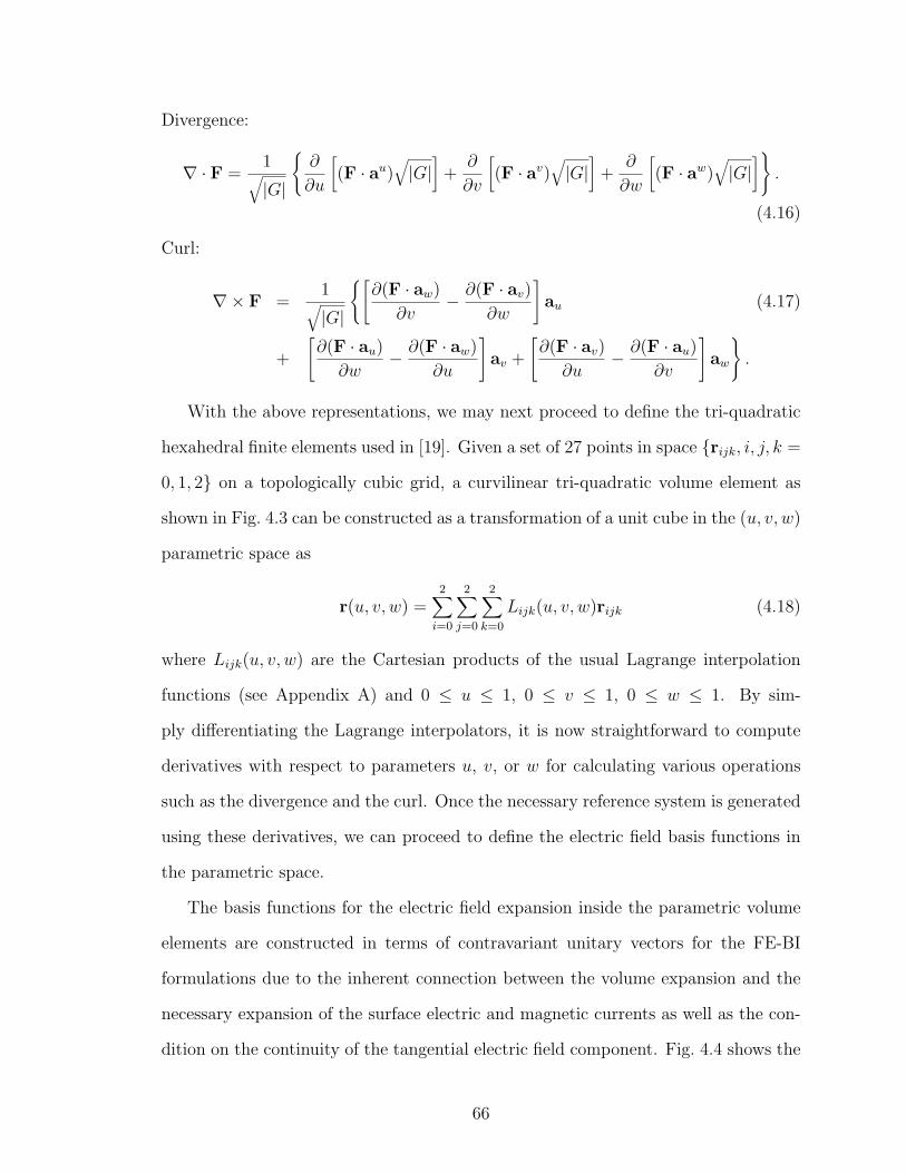
Divergence:

∇ · F =1√|G|

∂

∂u

[(F · au)

√|G|

]+

∂

∂v

[(F · av)

√|G|

]+

∂

∂w

[(F · aw)

√|G|

].

(4.16)

Curl:

∇× F =1√|G|

[∂(F · aw)

∂v− ∂(F · av)

∂w

]au (4.17)

+

[∂(F · au)

∂w− ∂(F · aw)

∂u

]av +

[∂(F · av)

∂u− ∂(F · au)

∂v

]aw

.

With the above representations, we may next proceed to define the tri-quadratic

hexahedral finite elements used in [19]. Given a set of 27 points in space rijk, i, j, k =

0, 1, 2 on a topologically cubic grid, a curvilinear tri-quadratic volume element as

shown in Fig. 4.3 can be constructed as a transformation of a unit cube in the (u, v, w)

parametric space as

r(u, v, w) =2∑

i=0

2∑

j=0

2∑

k=0

Lijk(u, v, w)rijk (4.18)

where Lijk(u, v, w) are the Cartesian products of the usual Lagrange interpolation

functions (see Appendix A) and 0 ≤ u ≤ 1, 0 ≤ v ≤ 1, 0 ≤ w ≤ 1. By sim-

ply differentiating the Lagrange interpolators, it is now straightforward to compute

derivatives with respect to parameters u, v, or w for calculating various operations

such as the divergence and the curl. Once the necessary reference system is generated

using these derivatives, we can proceed to define the electric field basis functions in

the parametric space.

The basis functions for the electric field expansion inside the parametric volume

elements are constructed in terms of contravariant unitary vectors for the FE-BI

formulations due to the inherent connection between the volume expansion and the

necessary expansion of the surface electric and magnetic currents as well as the con-

dition on the continuity of the tangential electric field component. Fig. 4.4 shows the

66

u

v

w

r000 r

100 r200

r001

r002

r210

r220

r211

r212

r221

Figure 4.3. Quadratic hexahedral finite element.

convention used to associate basis functions with the edges of the elements. For each

volume element, the 12 basis functions associated with the 12 edges of the element

are given by the covariant projection form

e1 = (v)(w)au, e2 = (1− v)(w)au, (4.19)

e3 = (v)(1− w)au, e4 = (1− v)(1− w)au,

e5 = (u)(w)av, e6 = (1− u)(w)av,

e7 = (u)(1− w)av, e8 = (1− u)(1− w)av,

e9 = (u)(v)aw, e10 = (1− u)(v)aw,

e11 = (u)(1− v)aw, e12 = (1− u)(1− v)aw.

These definitions ensure that the basis functions have the same tangential compo-

nents across the element faces, since each basis function is constructed over a set of

hexahedra sharing a common edge. Properly pairing the basis functions on neigh-

boring elements, as is done for the surface elements in Chapter 2, we construct the

volumetric basis function for the electric field expansion. A detailed discussion on

67

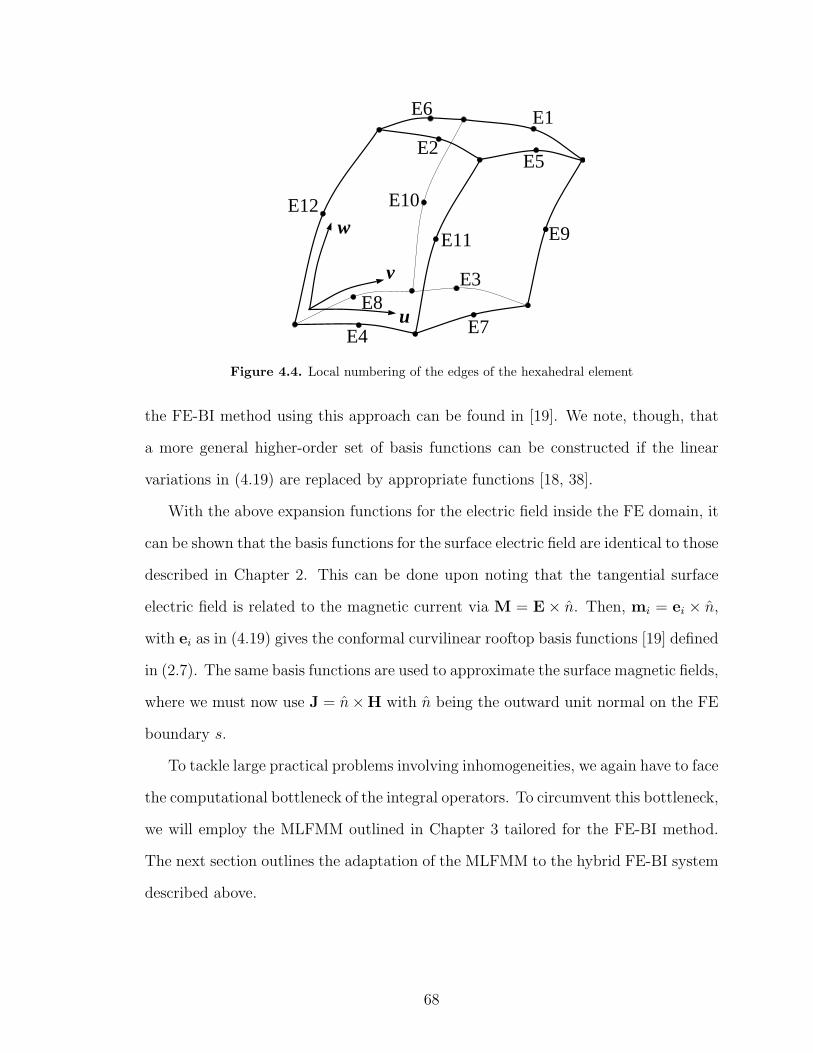
u

v

w

E1

E2

E3

E4

E5

E6

E7E8

E9

E10

E11

E12

Figure 4.4. Local numbering of the edges of the hexahedral element

the FE-BI method using this approach can be found in [19]. We note, though, that

a more general higher-order set of basis functions can be constructed if the linear

variations in (4.19) are replaced by appropriate functions [18, 38].

With the above expansion functions for the electric field inside the FE domain, it

can be shown that the basis functions for the surface electric field are identical to those

described in Chapter 2. This can be done upon noting that the tangential surface

electric field is related to the magnetic current via M = E × n. Then, mi = ei × n,

with ei as in (4.19) gives the conformal curvilinear rooftop basis functions [19] defined

in (2.7). The same basis functions are used to approximate the surface magnetic fields,

where we must now use J = n×H with n being the outward unit normal on the FE

boundary s.

To tackle large practical problems involving inhomogeneities, we again have to face

the computational bottleneck of the integral operators. To circumvent this bottleneck,

we will employ the MLFMM outlined in Chapter 3 tailored for the FE-BI method.

The next section outlines the adaptation of the MLFMM to the hybrid FE-BI system

described above.

68

4.3 MLFMM for FE-BI

If we assume that the outer boundary s of the solution domain v does not have a

perfectly magnetically conducting (PMC) boundary (which is the case for realistic

structures), we can make use of the fact that the tangential magnetic field being non-

zero over the entire surface s and tangential electric field being zero over the PEC

portions of s along with the fact that the same surface basis functions being used for

both tangential fields, to devise an efficient MLFMM approach.

For the general FE-BI formulation, two surface unknowns are needed for the

solution. These surface unknowns occupy the same physical location and thus a

single FMM clustering can be used to reduce CPU time and memory. Specifically,

we can use the clustering information for the surface magnetic field, i.e. n ×H for

the matrix [Q] and use the information in the matrix-vector product with the [P ]

matrix. Furthermore, since the same basis functions are used for both n × H and

E×n, only the signature functions for the tangential magnetic field basis functions (i.e.

electric currents) need to be computed. These two facts provide considerable memory

savings since the same translation operators and signature functions are reused for

both surface unknowns. Following the same approach as outlined in Chapter 3, we

decompose the far-field portions of the [P ] and [Q] matrices in the spectral domain

as

Pji ≈ ik

4π

∫d2kV

(P )jm (k) · TL(krmm′ , k · rmm′)V∗

im′(k), (4.20)

and

Qji ≈ ik

4π

∫d2kV

(Q)jm (k) · TL(krmm′ , k · rmm′)V∗

im′(k), (4.21)

with

V(P )jm (k) = −αV

(2)jm(k) + (1− α)V

(4)jm(k),

V(Q)jm (k) = αη0V

(1)jm(k) + (1− α)η0V

(3)jm(k), (4.22)

69

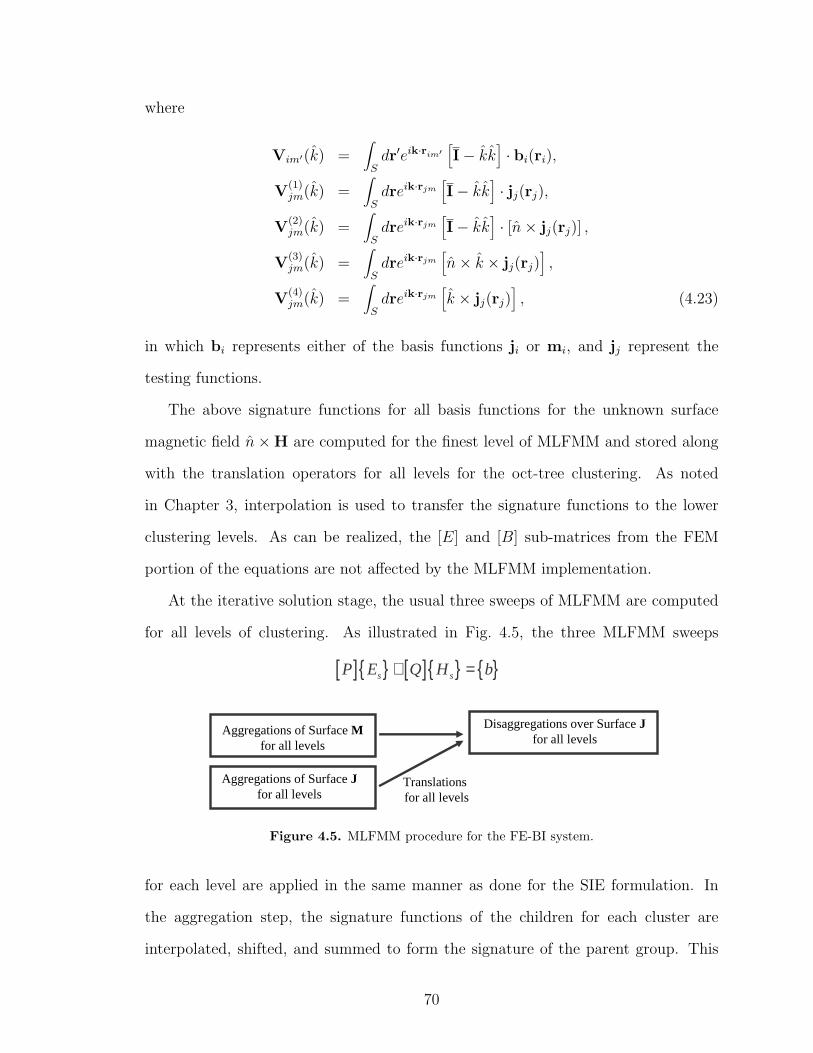
where

Vim′(k) =∫

Sdr′eik·rim′

[I− kk

]· bi(ri),

V(1)jm(k) =

∫

Sdreik·rjm

[I− kk

]· jj(rj),

V(2)jm(k) =

∫

Sdreik·rjm

[I− kk

]· [n× jj(rj)] ,

V(3)jm(k) =

∫

Sdreik·rjm

[n× k × jj(rj)

],

V(4)jm(k) =

∫

Sdreik·rjm

[k × jj(rj)

], (4.23)

in which bi represents either of the basis functions ji or mi, and jj represent the

testing functions.

The above signature functions for all basis functions for the unknown surface

magnetic field n×H are computed for the finest level of MLFMM and stored along

with the translation operators for all levels for the oct-tree clustering. As noted

in Chapter 3, interpolation is used to transfer the signature functions to the lower

clustering levels. As can be realized, the [E] and [B] sub-matrices from the FEM

portion of the equations are not affected by the MLFMM implementation.

At the iterative solution stage, the usual three sweeps of MLFMM are computed

for all levels of clustering. As illustrated in Fig. 4.5, the three MLFMM sweeps

Aggregations of Surface Mfor all levels

Aggregations of Surface Jfor all levels

Disaggregations over Surface Jfor all levels

Translations for all levels

[ ] [ ] s sP E Q H b+ =

Figure 4.5. MLFMM procedure for the FE-BI system.

for each level are applied in the same manner as done for the SIE formulation. In

the aggregation step, the signature functions of the children for each cluster are

interpolated, shifted, and summed to form the signature of the parent group. This

70

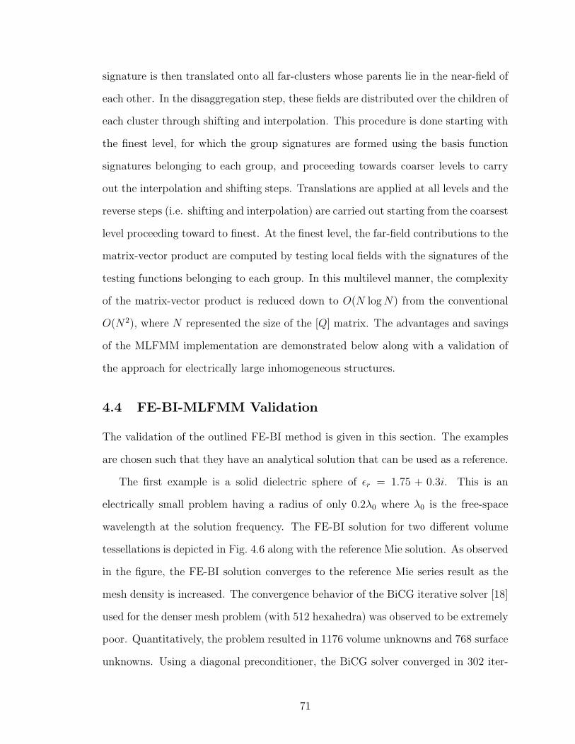
signature is then translated onto all far-clusters whose parents lie in the near-field of

each other. In the disaggregation step, these fields are distributed over the children of

each cluster through shifting and interpolation. This procedure is done starting with

the finest level, for which the group signatures are formed using the basis function

signatures belonging to each group, and proceeding towards coarser levels to carry

out the interpolation and shifting steps. Translations are applied at all levels and the

reverse steps (i.e. shifting and interpolation) are carried out starting from the coarsest

level proceeding toward to finest. At the finest level, the far-field contributions to the

matrix-vector product are computed by testing local fields with the signatures of the

testing functions belonging to each group. In this multilevel manner, the complexity

of the matrix-vector product is reduced down to O(N log N) from the conventional

O(N2), where N represented the size of the [Q] matrix. The advantages and savings

of the MLFMM implementation are demonstrated below along with a validation of

the approach for electrically large inhomogeneous structures.

4.4 FE-BI-MLFMM Validation

The validation of the outlined FE-BI method is given in this section. The examples

are chosen such that they have an analytical solution that can be used as a reference.

The first example is a solid dielectric sphere of εr = 1.75 + 0.3i. This is an

electrically small problem having a radius of only 0.2λ0 where λ0 is the free-space

wavelength at the solution frequency. The FE-BI solution for two different volume

tessellations is depicted in Fig. 4.6 along with the reference Mie solution. As observed

in the figure, the FE-BI solution converges to the reference Mie series result as the

mesh density is increased. The convergence behavior of the BiCG iterative solver [18]

used for the denser mesh problem (with 512 hexahedra) was observed to be extremely

poor. Quantitatively, the problem resulted in 1176 volume unknowns and 768 surface

unknowns. Using a diagonal preconditioner, the BiCG solver converged in 302 iter-

71

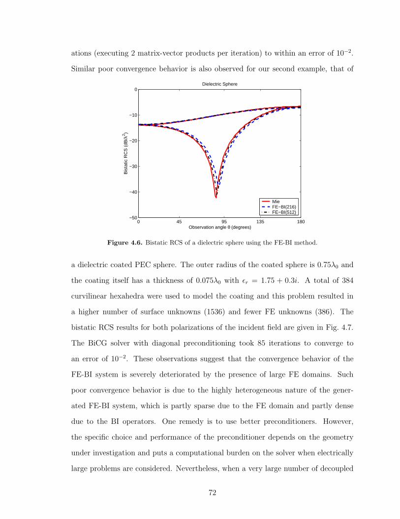
ations (executing 2 matrix-vector products per iteration) to within an error of 10−2.

Similar poor convergence behavior is also observed for our second example, that of

0 45 95 135 180−50

−40

−30

−20

−10

0

Observation angle θ (degrees)

Bis

tatic

RC

S (

dB/λ

2 )

Dielectric Sphere

MieFE−BI(216)FE−BI(512)

Figure 4.6. Bistatic RCS of a dielectric sphere using the FE-BI method.

a dielectric coated PEC sphere. The outer radius of the coated sphere is 0.75λ0 and

the coating itself has a thickness of 0.075λ0 with εr = 1.75 + 0.3i. A total of 384

curvilinear hexahedra were used to model the coating and this problem resulted in

a higher number of surface unknowns (1536) and fewer FE unknowns (386). The

bistatic RCS results for both polarizations of the incident field are given in Fig. 4.7.

The BiCG solver with diagonal preconditioning took 85 iterations to converge to

an error of 10−2. These observations suggest that the convergence behavior of the

FE-BI system is severely deteriorated by the presence of large FE domains. Such

poor convergence behavior is due to the highly heterogeneous nature of the gener-

ated FE-BI system, which is partly sparse due to the FE domain and partly dense

due to the BI operators. One remedy is to use better preconditioners. However,

the specific choice and performance of the preconditioner depends on the geometry

under investigation and puts a computational burden on the solver when electrically

large problems are considered. Nevertheless, when a very large number of decoupled

72

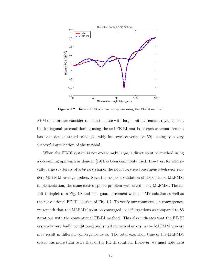
0 45 95 135 180−15

−10

−5

0

5

10

15

20

25

Observation angle θ (degrees)

Bis

tatic

RC

S (

dB/λ

2 )

Dielectric Coated PEC Sphere

MieFE−BI

Figure 4.7. Bistatic RCS of a coated sphere using the FE-BI method.

FEM domains are considered, as in the case with large finite antenna arrays, efficient

block diagonal preconditioning using the self FE-BI matrix of each antenna element

has been demonstrated to considerably improve convergence [59] leading to a very

successful application of the method.

When the FE-BI system is not exceedingly large, a direct solution method using

a decoupling approach as done in [19] has been commonly used. However, for electri-

cally large scatterers of arbitrary shape, the poor iterative convergence behavior ren-

ders MLFMM savings useless. Nevertheless, as a validation of the outlined MLFMM

implementation, the same coated sphere problem was solved using MLFMM. The re-

sult is depicted in Fig. 4.8 and is in good agreement with the Mie solution as well as

the conventional FE-BI solution of Fig. 4.7. To verify our comments on convergence,

we remark that the MLFMM solution converged in 112 iterations as compared to 85

iterations with the conventional FE-BI method. This also indicates that the FE-BI

system is very badly conditioned and small numerical errors in the MLFMM process

may result in different convergence rates. The total execution time of the MLFMM

solver was more than twice that of the FE-BI solution. However, we must note here

73

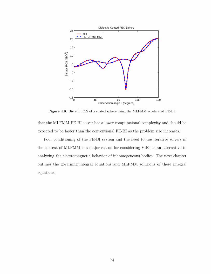
0 45 95 135 180−15

−10

−5

0

5

10

15

20

25

Observation angle θ (degrees)

Bis

tatic

RC

S (

dB/λ

2 )

Dielectric Coated PEC Sphere

MieFE−BI−MLFMM

Figure 4.8. Bistatic RCS of a coated sphere using the MLFMM accelerated FE-BI.

that the MLFMM-FE-BI solver has a lower computational complexity and should be

expected to be faster than the conventional FE-BI as the problem size increases.

Poor conditioning of the FE-BI system and the need to use iterative solvers in

the context of MLFMM is a major reason for considering VIEs as an alternative to

analyzing the electromagnetic behavior of inhomogeneous bodies. The next chapter

outlines the governing integral equations and MLFMM solutions of these integral

equations.

74

CHAPTER 5

Volume Integral Equations

Scattering by dielectric and composite volumes is of significant interest for radar

cross section (RCS) and electromagnetic compatibility/electromagnetic interference

(EMI/EMC) evaluation of modern composite vehicles and structures. Over the past

three decades several authors considered the scattering by dielectric volumes using

the MoM [30]. However, because the number of unknowns needed to formulate the

moment method for volumetric dielectrics quickly grows to many thousands, even

for a structure as small as 1λ3 in volume, the method is difficult to use for practical

applications. An alternative is to use a surface integral formulation for dielectrics [60],

but this is only applicable to piecewise–homogeneous structures. To alleviate the

O(N3) CPU bottleneck for modeling dielectric volumes, k-space methods utilizing

iterative solution approaches were introduced. However, by virtue of the FFT, these

often lack geometrical conformality.

With the recent success of fast methods, such as the MLFMM [8, 44], it is im-

portant to re-examine VIEs as an alternative to modeling inhomogeneous volumetric

structures (see [61] for an application of VIEs to indoor radio wave propagation). In

this chapter, we develop a VIE solution method using curvilinear hexahedral elements

for conformal modeling of penetrable structures and introduce a MLFMM solution of

the pertinent VIEs. It is demonstrated that even piecewise constant basis functions

provide excellent accuracy at a nominal sampling rates when conformal elements are

used. Results are given to show the accuracy of the method as well as the CPU and

75

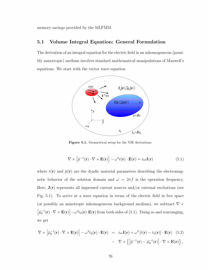
memory savings provided by the MLFMM.

5.1 Volume Integral Equation: General Formulation

The derivation of an integral equation for the electric field in an inhomogeneous (possi-

bly anisotropic) medium involves standard mathematical manipulations of Maxwell’s

equations. We start with the vector wave equation

ε (r), µ (r)0 0

vε(r), µ(r)

s=∂v

v0 s =∂v0 0

xy

z

(J r)

vs

E (r)inc

Figure 5.1. Geometrical setup for the VIE derivations.

∇×[µ−1(r) · ∇ × E(r)

]− ω2ε(r) · E(r) = iωJ(r) (5.1)

where ε(r) and µ(r) are the dyadic material parameters describing the electromag-

netic behavior of the solution domain and ω = 2πf is the operation frequency.

Here, J(r) represents all impressed current sources and/or external excitations (see

Fig. 5.1). To arrive at a wave equation in terms of the electric field in free space

(or possibly an anisotropic inhomogeneous background medium), we subtract ∇ ×[µ−1

0 (r) · ∇ × E(r)]−ω2ε0(r)·E(r) from both sides of (5.1). Doing so and rearranging,

we get

∇×[µ−1

0 (r) · ∇ × E(r)]− ω2ε0(r) · E(r) = iωJ(r) + ω2 [ε(r)− ε0(r)] · E(r) (5.2)

− ∇×[

µ−1(r)− µ−10 (r)

]· ∇ × E(r)

,

76

in which ε0(r) = ε0I and µ0(r) = µ0I refer to the permittivity and permeability of

the background medium, chosen as free-space here, and I is the identity dyad. The

right hand side of (5.2) can now be identified as a source term and accounts for the

presence of the inhomogeneous medium. The solution for E(r) can now be carried

out using the dyadic Green’s function satisfying

∇×[µ−1

0 (r) · ∇ ×G(r, r′)]− ω2ε0(r) ·G(r, r′) = µ−1

0 (r)δ(r− r′). (5.3)

The Green’s function takes the well-known form

G(r, r′) =

(I +

1

k20

∇∇)

g(r, r′), g(r, r′) =eik0|r−r′|

|r− r′| , (5.4)

where k0 = ω√

ε0µ0. Using the right hand side of (5.2) as the source, we readily

obtain [62]

E(r) = iωµ0

∫

v+v0

dr′G(r, r′) · J(r′) (5.5)

+ k20

∫

v+v0

dr′G(r, r′) · (εr(r′)− I) · E(r′)

−∫

v+v0

dr′G(r, r′) · ∇′ ×[(

µ−1r (r′)− I

)· ∇′ × E(r′)

]

where εr = ε/ε0 and µr = µ/µ0. The first term in the above is identified as the

excitation field generated by the main J(r), viz.

Einc(r) = iωµ0

∫

vs

dr′G(r, r′) · J(r′) (5.6)

where the integration domain (v + v0) is conveniently replaced by vs since this repre-

sents the only volume over which J(r) is non-zero. The other two terms vanish when

ε(r) = ε0I, µ(r) = µ0I and consequently represent the scattering due to v.

To relax the differentiability requirement on(µ−1

r (r)− I)·∇′×E(r′) in the third

term in (5.5), we can make use of the divergence theorem (n is outward from v)

∫

vdr∇ ·

[G× y

]=

∮

sdrn ·

[G× y

]=

∮

sdrG · (n× y) (5.7)

77

and the dyadic identity

∇ ·[G× y

]= G · ∇ × y −∇×G · y (5.8)

where y is an arbitrary vector chosen here to be y =(µ−1

r (r)− I)· ∇′ ×E(r′). This

manipulation leads to

E(r) = Einc(r) + k20

∫

v+v0

dr′G(r, r′) · (εr(r′)− I) · E(r′) (5.9)

−∫

v+v0

dr′∇′ ×G(r, r′) ·[(

µ−1r (r′)− I

)· ∇′ × E(r′)

]

+∮

s0

dr′G(r, r′) · n′ ×[(

µ−1r (r′)− I

)· ∇′ × E(r′)

].

In comparison to (5.5), this does not include any differentiation on(µ−1

r (r′)− I)·∇′×

E(r′). However, a surface integral is introduced for enclosing v + v0. As s0 →∞, the

radiation condition implies that the surface integral vanishes, giving

E(r) = Einc(r) + k20

∫

v+v0

dr′G(r, r′) · (εr(r′)− I) · E(r′) (5.10)

−∫

v+v0

dr′∇′ ×G(r, r′) ·[(

µ−1r (r′)− I

)· ∇′ × E(r′)

].

An alternative way to derive (5.10) is through the standard use of equivalent

electric and magnetic currents. In accordance with [27], we could introduce the

volumetric electric and magnetic current density sources

Jeq(r) = −iωε0

[εr(r)− I

]· E(r), Meq(r) = −

[µr(r)− I

]·H(r) (5.11)

to represent the scattering by the dielectric volume. These sources radiate (in free

space) and are responsible for the scattered fields

Escat(r) = iωµ0

∫

vdr′

[G(r, r′) · Jeq(r

′) +∇′ ×G(r, r′) ·Meq(r′)

](5.12)

and

E(r) = Einc(r) + Escat(r) (5.13)

with the dual expressions valid for Hscat(r). Equation (5.13) and its dual yield a

pair of integral equations for the solution of the unknown volume equivalent currents

Jeq(r) and Meq(r) (or H(r) and E(r), respectively).

78

The above formulation involving equivalent volume currents was used by Rich-

mond [29] for two dimensional applications, and results in six scalar unknowns per

volume location for problems involving having non-trivial permittivity and perme-

ability. In contrast, (5.10) involves only a single vector field unknown (three scalar

unknowns) per volume location. However, (5.10) requires differentiation (curl) of the

unknown field E(r) in much the same way done in the finite element method [18].

One could actually choose to remove the differentiation from E(r) but would then

obtain an integrand which involves differentiation of the permeability across the vol-

ume. This was done in [32] and although the final expression avoids the curl of the

unknown E(r), the need to differentiate µr(r) is undesirable for numerical implemen-

tation when µr(r) is not available in analytic form. Clearly, among the representations

(5.10), (5.12), and Equation (28) of [32], the one given by (5.10) is most attractive

for numerical implementation.

5.2 MoM formulation of the VIE for dielectrics

For the specific case when we are dealing only with a dielectric inhomogeneity (µr =

1), (5.10) simplifies to

E(r) = Einc(r) + k20

∫

vdr′G(r, r′) · (εr(r

′)− I) · E(r′). (5.14)

We proceed with the standard MoM expansion of the unknown electric field intensity

E as

E(r) =N∑

i=1

xiei(r) (5.15)

and Galerkin’s testing to arrive at a matrix equation [Z]x = b where,

Zji = 〈ej(r), ei(r)〉 − k20〈ej(r),

∫

vdr′G(r, r′) ·

(εr − I

)· ei(r

′)〉. (5.16)

The right hand side of the matrix system in the parametric space takes the form bj =

〈ej(r),Einc(r)〉. Similar to the SIE implementation, the hyper-singularity in (5.16) is

79

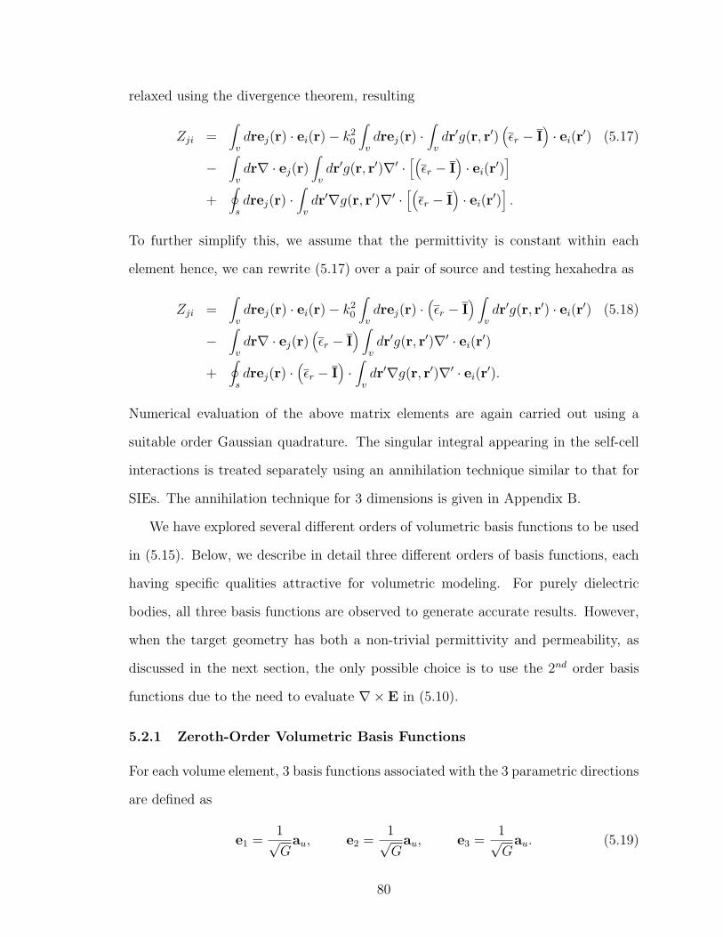
relaxed using the divergence theorem, resulting

Zji =∫

vdrej(r) · ei(r)− k2

0

∫

vdrej(r) ·

∫

vdr′g(r, r′)

(εr − I

)· ei(r

′) (5.17)

−∫

vdr∇ · ej(r)

∫

vdr′g(r, r′)∇′ ·

[(εr − I

)· ei(r

′)]

+∮

sdrej(r) ·

∫

vdr′∇g(r, r′)∇′ ·

[(εr − I

)· ei(r

′)].

To further simplify this, we assume that the permittivity is constant within each

element hence, we can rewrite (5.17) over a pair of source and testing hexahedra as

Zji =∫

vdrej(r) · ei(r)− k2

0

∫

vdrej(r) ·

(εr − I

) ∫

vdr′g(r, r′) · ei(r

′) (5.18)

−∫

vdr∇ · ej(r)

(εr − I

) ∫

vdr′g(r, r′)∇′ · ei(r

′)

+∮

sdrej(r) ·

(εr − I

)·∫

vdr′∇g(r, r′)∇′ · ei(r

′).

Numerical evaluation of the above matrix elements are again carried out using a

suitable order Gaussian quadrature. The singular integral appearing in the self-cell

interactions is treated separately using an annihilation technique similar to that for

SIEs. The annihilation technique for 3 dimensions is given in Appendix B.

We have explored several different orders of volumetric basis functions to be used

in (5.15). Below, we describe in detail three different orders of basis functions, each

having specific qualities attractive for volumetric modeling. For purely dielectric

bodies, all three basis functions are observed to generate accurate results. However,

when the target geometry has both a non-trivial permittivity and permeability, as

discussed in the next section, the only possible choice is to use the 2nd order basis

functions due to the need to evaluate ∇× E in (5.10).

5.2.1 Zeroth-Order Volumetric Basis Functions

For each volume element, 3 basis functions associated with the 3 parametric directions

are defined as

e1 =1√G

au, e2 =1√G

au, e3 =1√G

au. (5.19)

80

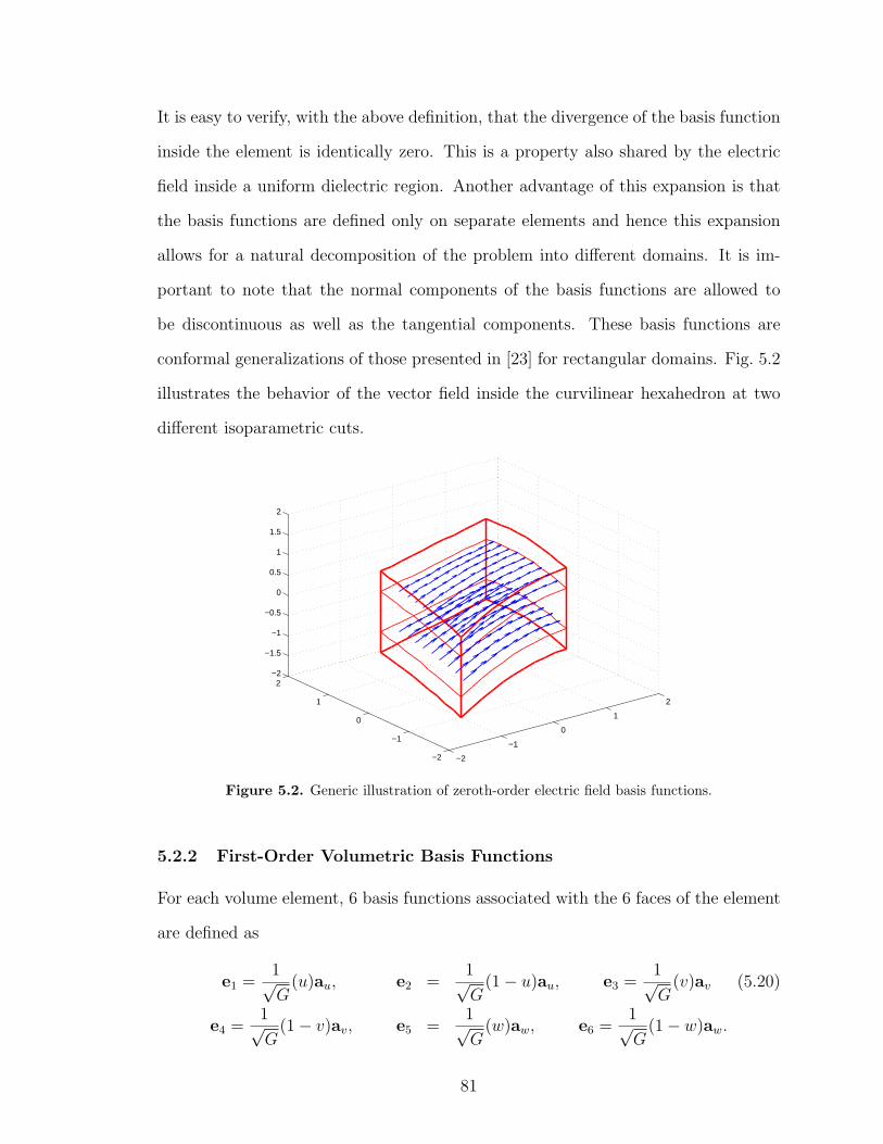
It is easy to verify, with the above definition, that the divergence of the basis function

inside the element is identically zero. This is a property also shared by the electric

field inside a uniform dielectric region. Another advantage of this expansion is that

the basis functions are defined only on separate elements and hence this expansion

allows for a natural decomposition of the problem into different domains. It is im-

portant to note that the normal components of the basis functions are allowed to

be discontinuous as well as the tangential components. These basis functions are

conformal generalizations of those presented in [23] for rectangular domains. Fig. 5.2

illustrates the behavior of the vector field inside the curvilinear hexahedron at two

different isoparametric cuts.

−2

−1

0

1

2

−2

−1

0

1

2−2

−1.5

−1

−0.5

0

0.5

1

1.5

2

Figure 5.2. Generic illustration of zeroth-order electric field basis functions.

5.2.2 First-Order Volumetric Basis Functions

For each volume element, 6 basis functions associated with the 6 faces of the element

are defined as

e1 =1√G

(u)au, e2 =1√G

(1− u)au, e3 =1√G

(v)av (5.20)

e4 =1√G

(1− v)av, e5 =1√G

(w)aw, e6 =1√G

(1− w)aw.

81

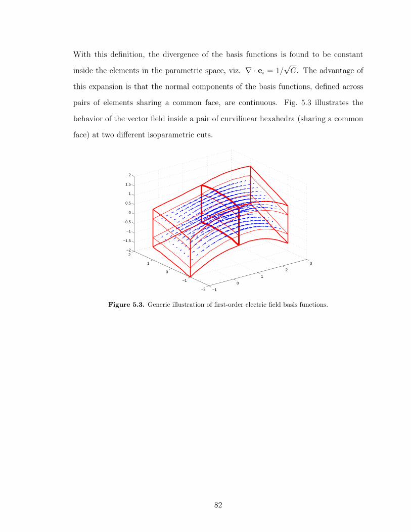
With this definition, the divergence of the basis functions is found to be constant

inside the elements in the parametric space, viz. ∇ · ei = 1/√

G. The advantage of

this expansion is that the normal components of the basis functions, defined across

pairs of elements sharing a common face, are continuous. Fig. 5.3 illustrates the

behavior of the vector field inside a pair of curvilinear hexahedra (sharing a common

face) at two different isoparametric cuts.

−1

0

1

2

3

−2

−1

0

1

2−2

−1.5

−1

−0.5

0

0.5

1

1.5

2

Figure 5.3. Generic illustration of first-order electric field basis functions.

82

5.2.3 Second-Order Volumetric Basis Functions

For each volume element, 12 basis functions associated with the 12 edges of the

element are defined as

e1 =1√G

(v)(w)au, e2 =1√G

(1− v)(w)au, (5.21)

e3 =1√G

(v)(1− w)au, e4 =1√G

(1− v)(1− w)au,

e5 =1√G

(u)(w)av, e6 =1√G

(1− u)(w)av,

e7 =1√G

(u)(1− w)av, e8 =1√G

(1− u)(1− w)av,

e9 =1√G

(u)(v)aw, e10 =1√G

(1− u)(v)aw,

e11 =1√G

(u)(1− v)aw, e12 =1√G

(1− u)(1− v)aw.

Switching to a covariant unitary vector expansion for the VIE formulation as opposed

to a contravariant form as in FE-BI basis functions has the advantage of providing

zero divergence inside the element and is the main reason for choosing it. As in the

case with zeroth-order basis functions, this property conforms with that of the electric

field. As opposed to a contravariant expansion (i.e. a covariant projection form), this

expansion does not have continuous tangential components across the common faces

of the elements that share a common edge. Fig. 5.4 illustrates the behavior of the

vector field inside a pair of curvilinear hexahedra (sharing a common edge) at two

different isoparametric cuts.

5.2.4 Validations for Dielectric Structures

Here, we show that all three different orders of volumetric basis functions defined

above produce accurate results. As a test geometry, a dielectric spherical shell is

considered. Fig. 5.5 depicts the computed RCS values for a dielectric shell of outer

radius 0.2λ0 and of thickness 0.02λ0. All three results agree well with the analytical

solution. However, we must note here that, although the same volume mesh is used

83

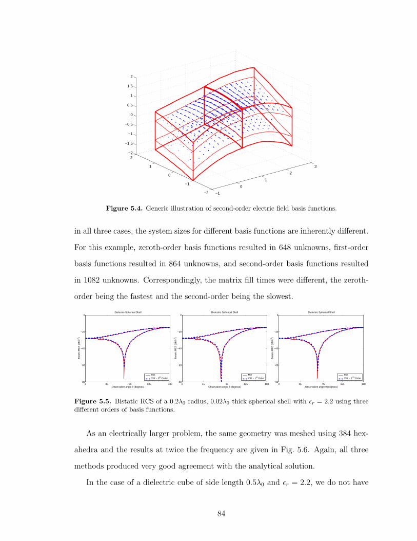
−1

0

1

2

3

−2

−1

0

1

2−2

−1.5

−1

−0.5

0

0.5

1

1.5

2

Figure 5.4. Generic illustration of second-order electric field basis functions.

in all three cases, the system sizes for different basis functions are inherently different.

For this example, zeroth-order basis functions resulted in 648 unknowns, first-order

basis functions resulted in 864 unknowns, and second-order basis functions resulted

in 1082 unknowns. Correspondingly, the matrix fill times were different, the zeroth-

order being the fastest and the second-order being the slowest.

0 45 95 135 180−80

−60

−40

−20

0

Observation angle θ (degrees)

Bis

tatic

RC

S (

dB/λ

2 )

Dielectric Spherical Shell

MieVIE − 0th Order

0 45 95 135 180−80

−60

−40

−20

0

Observation angle θ (degrees)

Bis

tatic

RC

S (

dB/λ

2 )

Dielectric Spherical Shell

MieVIE − 1st Order

0 45 95 135 180−80

−60

−40

−20

0

Observation angle θ (degrees)

Bis

tatic

RC

S (

dB/λ

2 )

Dielectric Spherical Shell

MieVIE − 2nd Order

Figure 5.5. Bistatic RCS of a 0.2λ0 radius, 0.02λ0 thick spherical shell with εr = 2.2 using threedifferent orders of basis functions.

As an electrically larger problem, the same geometry was meshed using 384 hex-

ahedra and the results at twice the frequency are given in Fig. 5.6. Again, all three

methods produced very good agreement with the analytical solution.

In the case of a dielectric cube of side length 0.5λ0 and εr = 2.2, we do not have

84

0 45 95 135 180−40

−30

−20

−10

0

10

Observation angle θ (degrees)

Bis

tatic

RC

S (

dB/λ

2 )

Dielectric Spherical Shell

MieVIE − 0th Order

0 45 95 135 180−40

−30

−20

−10

0

10

Observation angle θ (degrees)

Bis

tatic

RC

S (

dB/λ

2 )

Dielectric Spherical Shell

MieVIE − 1st Order

0 45 95 135 180−40

−30

−20

−10

0

10

Observation angle θ (degrees)

Bis

tatic

RC

S (

dB/λ

2 )

Dielectric Spherical Shell

MieVIE − 2nd Order

Figure 5.6. Bistatic RCS of a 0.4λ0 radius, 0.04λ0 thick spherical shell with εr = 2.2 using threedifferent orders of basis functions.

a closed form reference solution. However, the bistatic RCS of the dielectric cube

using three different orders of basis functions is plotted in Fig. 5.7 and all results are

observed to be in good to fair agreement.

0 45 95 135 180−50

−40

−30

−20

−10

0

Observation angle θ (degrees)

Bis

tatic

RC

S (

dB/λ

2 )

Dielectric Cube

0th Order1st Order2nd Order

Figure 5.7. Bistatic RCS of a 0.5λ0 side length dielectric cube with εr = 2.2 using three differentorders of basis functions.

The three examples given above demonstrate that for dielectric scatterers the

present integral equation solutions produce accurate RCS results regardless of the

expansion order for the unknown electric field intensity. Based on this conclusion, we

will adopt the lowest order basis function in the MLFMM implementation for volu-

metric dielectric bodies. This also allows for a physical domain decomposition since

85

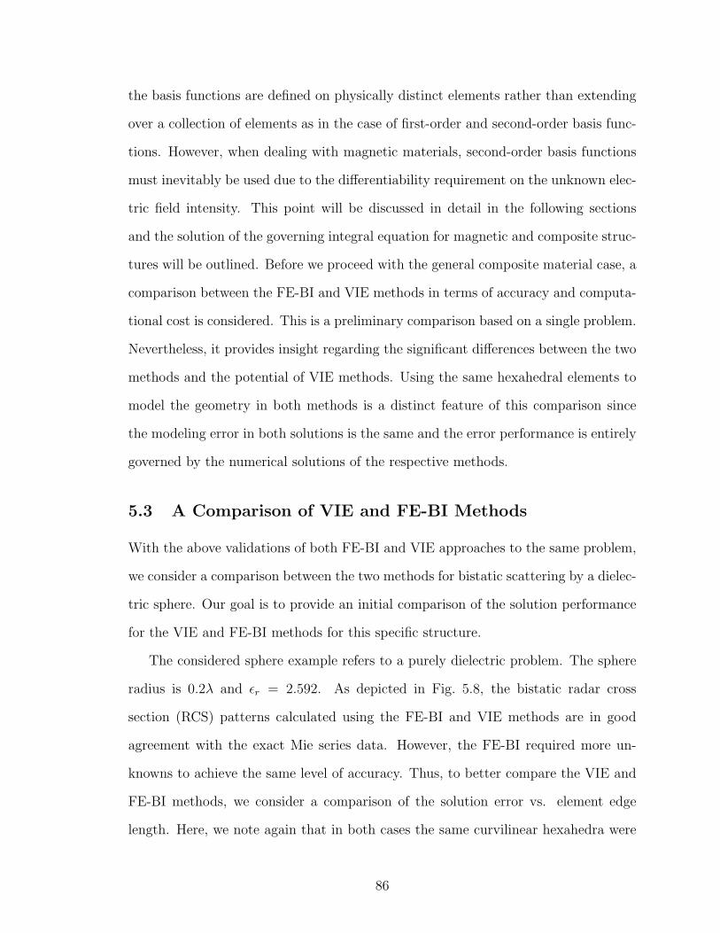
the basis functions are defined on physically distinct elements rather than extending

over a collection of elements as in the case of first-order and second-order basis func-

tions. However, when dealing with magnetic materials, second-order basis functions

must inevitably be used due to the differentiability requirement on the unknown elec-

tric field intensity. This point will be discussed in detail in the following sections

and the solution of the governing integral equation for magnetic and composite struc-

tures will be outlined. Before we proceed with the general composite material case, a

comparison between the FE-BI and VIE methods in terms of accuracy and computa-

tional cost is considered. This is a preliminary comparison based on a single problem.

Nevertheless, it provides insight regarding the significant differences between the two

methods and the potential of VIE methods. Using the same hexahedral elements to

model the geometry in both methods is a distinct feature of this comparison since

the modeling error in both solutions is the same and the error performance is entirely

governed by the numerical solutions of the respective methods.

5.3 A Comparison of VIE and FE-BI Methods

With the above validations of both FE-BI and VIE approaches to the same problem,

we consider a comparison between the two methods for bistatic scattering by a dielec-

tric sphere. Our goal is to provide an initial comparison of the solution performance

for the VIE and FE-BI methods for this specific structure.

The considered sphere example refers to a purely dielectric problem. The sphere

radius is 0.2λ and εr = 2.592. As depicted in Fig. 5.8, the bistatic radar cross

section (RCS) patterns calculated using the FE-BI and VIE methods are in good

agreement with the exact Mie series data. However, the FE-BI required more un-

knowns to achieve the same level of accuracy. Thus, to better compare the VIE and

FE-BI methods, we consider a comparison of the solution error vs. element edge

length. Here, we note again that in both cases the same curvilinear hexahedra were

86

used. This comparison was done for the sphere example and resulted in the curves

given in Fig. 5.9. They depict that the error is proportional to the square of the

element’s edge length for both methods. However, the VIE can afford larger elements

for the same error (∆V IE ≈√

2∆FE−BI). Also, as shown in Tab. 5.1, the VIE system

converges much faster but the matrix fill time is significantly higher. The latter is

a clear disadvantage of the VIE method, but the rapid convergence of its associated

matrix system provides incentives for further examination of the method. It should

be noted from Fig. 5.10 that the convergence behavior of FE-BI as a function of sys-

tem size scales linearly, whereas for this problem the VIE convergence is much faster

and almost independent of the rank of the matrix. This can be attributed to the

fact that the FE-BI system is highly heterogeneous and thus the generated matrix

is ill-conditioned, whereas the VIE is a second kind integral equation producing a

well-conditioned matrix.

0 45 95 135 180−40

−30

−20

−10

0

Observation Angle θ (Degrees.)

Bis

tatic

RC

S (

dB/λ

2 )

Dielectric Sphere

MieVIE (300)VIE (882)

0 45 95 135 180−40

−30

−20

−10

0

Observation Angle θ (Degrees.)

Bis

tatic

RC

S (

dB/λ

2 )

Dielectric Sphere

MieFE−BI (N = 492)FE−BI (N = 1314)

(a) (b)

Figure 5.8. Bistatic RCS of a dielectric sphere of radius 0.2λ (εr = 2.592). (a) VIE Solution,(b) FE-BI Solution.

Fig. 5.11 depicts the percent error in the RCS solution for the same sphere as a

function of the resulting systems for both methods. The VIE is again observed to

have a better performance for a fixed system size.

On the basis of the above example, we can remark that the FE-BI method will

87

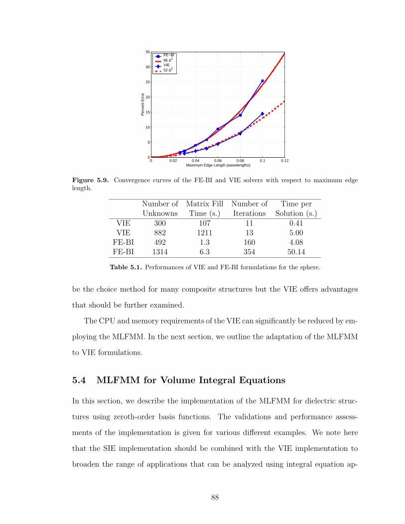
0 0.02 0.04 0.06 0.08 0.1 0.120

5

10

15

20

25

30

35

Maximum Edge Length (wavelengths)

Per

cent

Err

or

FE−BI96 ∆2

VIE52 ∆2

Figure 5.9. Convergence curves of the FE-BI and VIE solvers with respect to maximum edgelength.

Number of Matrix Fill Number of Time perUnknowns Time (s.) Iterations Solution (s.)

VIE 300 107 11 0.41VIE 882 1211 13 5.00

FE-BI 492 1.3 160 4.08FE-BI 1314 6.3 354 50.14

Table 5.1. Performances of VIE and FE-BI formulations for the sphere.

be the choice method for many composite structures but the VIE offers advantages

that should be further examined.

The CPU and memory requirements of the VIE can significantly be reduced by em-

ploying the MLFMM. In the next section, we outline the adaptation of the MLFMM

to VIE formulations.

5.4 MLFMM for Volume Integral Equations

In this section, we describe the implementation of the MLFMM for dielectric struc-

tures using zeroth-order basis functions. The validations and performance assess-

ments of the implementation is given for various different examples. We note here

that the SIE implementation should be combined with the VIE implementation to

broaden the range of applications that can be analyzed using integral equation ap-

88

0 500 1000 1500 2000 2500 3000 3500 40000

100

200

300

400

500

600

700

800

900

1000

Number of Unknowns

Num

ber

of It

erat

ions

FE−BIVIE

Figure 5.10. Iterative convergence of FE-BI and VIE solvers with respect to system size.

0 500 1000 1500 2000 2500 3000 3500 40000

5

10

15

20

25

30

Number of Unknowns

Per

cent

Err

or

FE−BIVIE

Figure 5.11. Error in FE-BI and VIE methods with respect to number of unknowns.

proaches.

So far, the MLFMM has been applied in the context of SIE formulations both

for impenetrable (PEC) target geometries [13] and FE–BI formulations of inhomoge-

neous penetrable targets [43]. Here, we apply the MLFMM to the VIE formulations

outlined above. To point out the potential of MLFMM as applied to VIEs, let us

consider a sphere of unit radius. In proceeding with the numerical SIE solution, a

meshing package, such as the MSC-PATRANr finite element mesher, is first used to pro-

duce a surface mesh consisting of, e.g., quadrilateral elements or triangular elements.

The size of the surface elements is determined by the wavelength of interest (the rule

89

of thumb is 10 elements per linear wavelength) and the resulting numerical system

dimension is proportional to the number of elements in the mesh. As a function of

element size ∆, the data in Table 5.2 were produced from the MSC-PATRANr’s mesher.

When the same gridding package is used to generate a volumetric mesh, the number

∆ Quadrilaterals Triangles0.250 150 3000.200 216 4320.150 384 7680.100 864 17280.075 1536 30720.050 3750 75000.040 5766 11532

Table 5.2. Surface mesh for a sphere.

of resulting finite elements are given in Table 5.3 as a function of the specified maxi-

mum edge length. Two observations can be made between Tables 5.2 and 5.3. First,

the number of tetrahedra needed for the same discretization rate is much larger (five

times larger) and thus tetrahedral meshing leads to many more unknowns. Second, in

comparing Tables 5.2 and 5.3, the number of unknowns grow dramatically for volume

formulations. Specifically, for volume formulations, the number of unknowns is pro-

portional to 1/∆3 as compared to 1/∆2 for surface formulations. For high contrast

dielectrics, ∆ ≈ λ/10√

εr must necessarily be smaller and this further exacerbates the

situation. Therefore, for VIE formulations, the problem size quickly grows to many

∆ Hexahedra Tetrahedra0.250 125 6250.200 216 10800.150 512 25600.100 1728 86400.075 4096 204800.050 15625 781250.040 29791 148955

Table 5.3. Volumetric mesh for a sphere.

90

thousands, even for a physically small geometry. To overcome the high computational

demands of VIEs, one must resort to more efficient strategies, like the MLFMM for

solving the MoM matrix.

Core equations of the MLFMM algorithm were presented in Chapter 3. Sum-

marizing, far-zone elements in (5.18), upon discretizing the spectral integral using

numerical quadrature (see [8]) are

Zji = − ik

4π

∑

k

wkVjm(k) TL(krmm′ , k · rmm′)V∗im′(k) (5.22)

where

Vjm(k) =∫

vdv′eik·rjm

[I− kk

]ej(rjm) (5.23)

and

Vim′(k) =∫

vdv′eik·rim′

[I− kk

]ei(rim′) (5.24)

are the signature functions. As seen, the only difference between the SIE-MLFMM

signature functions and the VIE-MLFMM signature functions is the domains of the

integration. By merely incorporating these signatures in the MLFMM algorithm as

outlined for SIEs, we can adapt the MLFMM to VIEs.

Once the signature functions for each basis function are computed and stored, the

rest of the MLFMM algorithm is identical to that of a surface formulation discussed

in Chapter 3. However, the MLFMM parameters must be re-adjusted for optimal

performance since the unknowns are distributed in a volume, rather than on a sur-

face. Consequently, the cost of the MLFMM part in the matrix-vector product for the

near-field section of the matrix will differ from that of the SIE-MLFMM solver. A fine

tuning of the implementation is also necessary if different clustering approaches must

be employed, since the MLFMM performance relies heavily on the clustering setup.

For example, the MLFMM parameters (i.e. the number of multipoles and the band-

width of the near–field matrix) are predetermined using the size and neighborhood

information of the clusters. Furthermore, clustering information must be utilized for

91

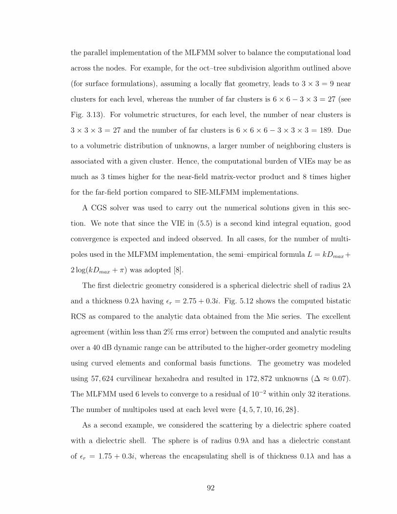
the parallel implementation of the MLFMM solver to balance the computational load

across the nodes. For example, for the oct–tree subdivision algorithm outlined above

(for surface formulations), assuming a locally flat geometry, leads to 3 × 3 = 9 near

clusters for each level, whereas the number of far clusters is 6 × 6 − 3 × 3 = 27 (see

Fig. 3.13). For volumetric structures, for each level, the number of near clusters is

3 × 3 × 3 = 27 and the number of far clusters is 6 × 6 × 6 − 3 × 3 × 3 = 189. Due

to a volumetric distribution of unknowns, a larger number of neighboring clusters is

associated with a given cluster. Hence, the computational burden of VIEs may be as

much as 3 times higher for the near-field matrix-vector product and 8 times higher

for the far-field portion compared to SIE-MLFMM implementations.

A CGS solver was used to carry out the numerical solutions given in this sec-

tion. We note that since the VIE in (5.5) is a second kind integral equation, good

convergence is expected and indeed observed. In all cases, for the number of multi-

poles used in the MLFMM implementation, the semi–empirical formula L = kDmax+

2 log(kDmax + π) was adopted [8].

The first dielectric geometry considered is a spherical dielectric shell of radius 2λ

and a thickness 0.2λ having εr = 2.75 + 0.3i. Fig. 5.12 shows the computed bistatic

RCS as compared to the analytic data obtained from the Mie series. The excellent

agreement (within less than 2% rms error) between the computed and analytic results

over a 40 dB dynamic range can be attributed to the higher-order geometry modeling

using curved elements and conformal basis functions. The geometry was modeled

using 57, 624 curvilinear hexahedra and resulted in 172, 872 unknowns (∆ ≈ 0.07).

The MLFMM used 6 levels to converge to a residual of 10−2 within only 32 iterations.

The number of multipoles used at each level were 4, 5, 7, 10, 16, 28.As a second example, we considered the scattering by a dielectric sphere coated

with a dielectric shell. The sphere is of radius 0.9λ and has a dielectric constant

of εr = 1.75 + 0.3i, whereas the encapsulating shell is of thickness 0.1λ and has a

92

0 45 95 135 180−10

0

10

20

30

40

50

Observation Angle (Degrees)

Bis

tatic

RC

S (

dB/λ

2 )

Dielectric Spherical Shell

MieVIE

r1r2

1ε

Figure 5.12. Bistatic RCS of a 2λ radius dielectric spherical shell (εr = 2.75 + 0.3i).

dielectric constant of εr = 1.25 + 1.25i. This geometry was modeled using 23, 125

elements (69, 375 unknowns), and the simulation was done using 5 MLFMM levels.

The CGS solver converged in 231 iterations and the number of multipoles used for

this example were 4, 5, 7, 10, 16. Again, we observe the remarkably fast convergence

rate, and accuracy (within less than 2.5% rms error) using nominal sampling (see

Fig. 5.13).

Our final example demonstrates the accuracy of the method for high contrast

dielectric materials. The geometry is a two-layer material coated sphere with the

permittivity of the sphere’s core being εr1 = 1.25 up to a radius of 0.18λ0, λ0 being

the free-space wavelength. For the first layer coating, the thickness is 0.02λ0 and

εr2 = 15.0 representing a contrast of 12 to 1 at the boundary between the layer and the

sphere’s core. The outermost layer also has a thickness of 0.02λ0 and a permittivity

εr3. Considering the wavelength in the high permittivity shell (εr2 = 15.0), the

volumetric mesh for this region is constructed by specifying the maximum edge length

to be around (λ0/10)/√

εr2 ≈ 0.0258λ0. The rest of the volume mesh is necessarily

93

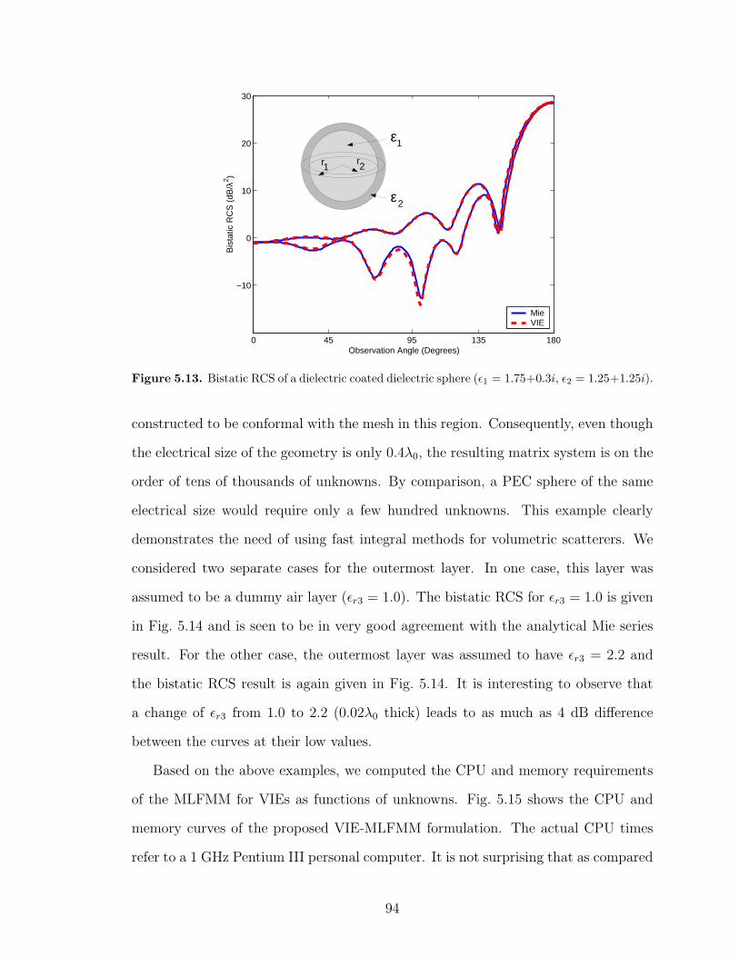
0 45 95 135 180

−10

0

10

20

30

Observation Angle (Degrees)

Bis

tatic

RC

S (

dB/λ

2 )

MieVIE

r1r2

1ε

2ε

Figure 5.13. Bistatic RCS of a dielectric coated dielectric sphere (ε1 = 1.75+0.3i, ε2 = 1.25+1.25i).

constructed to be conformal with the mesh in this region. Consequently, even though

the electrical size of the geometry is only 0.4λ0, the resulting matrix system is on the

order of tens of thousands of unknowns. By comparison, a PEC sphere of the same

electrical size would require only a few hundred unknowns. This example clearly

demonstrates the need of using fast integral methods for volumetric scatterers. We

considered two separate cases for the outermost layer. In one case, this layer was

assumed to be a dummy air layer (εr3 = 1.0). The bistatic RCS for εr3 = 1.0 is given

in Fig. 5.14 and is seen to be in very good agreement with the analytical Mie series

result. For the other case, the outermost layer was assumed to have εr3 = 2.2 and

the bistatic RCS result is again given in Fig. 5.14. It is interesting to observe that

a change of εr3 from 1.0 to 2.2 (0.02λ0 thick) leads to as much as 4 dB difference

between the curves at their low values.

Based on the above examples, we computed the CPU and memory requirements

of the MLFMM for VIEs as functions of unknowns. Fig. 5.15 shows the CPU and

memory curves of the proposed VIE-MLFMM formulation. The actual CPU times

refer to a 1 GHz Pentium III personal computer. It is not surprising that as compared

94

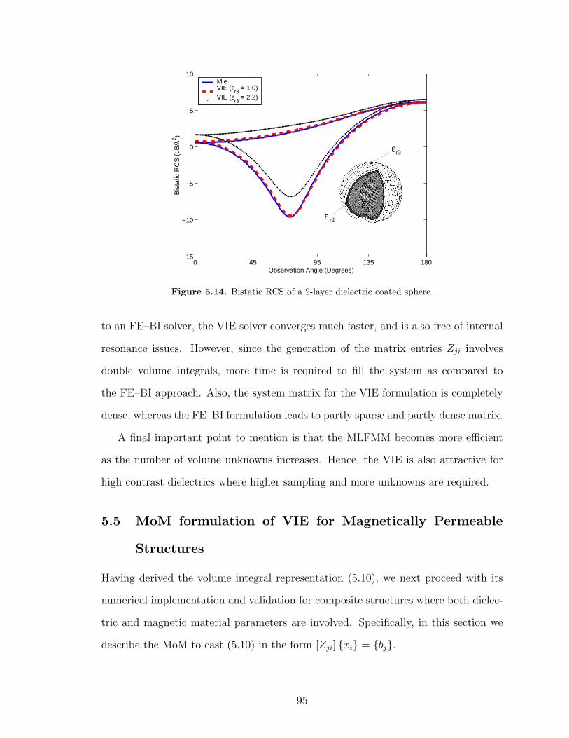
0 45 95 135 180−15

−10

−5

0

5

10

Observation Angle (Degrees)

Bis

tatic

RC

S (

dB/λ

2 )

MieVIE (ε

r3 = 1.0)

VIE (εr3

= 2.2)

r2ε

r3ε

εr1

Figure 5.14. Bistatic RCS of a 2-layer dielectric coated sphere.

to an FE–BI solver, the VIE solver converges much faster, and is also free of internal

resonance issues. However, since the generation of the matrix entries Zji involves

double volume integrals, more time is required to fill the system as compared to

the FE–BI approach. Also, the system matrix for the VIE formulation is completely

dense, whereas the FE–BI formulation leads to partly sparse and partly dense matrix.

A final important point to mention is that the MLFMM becomes more efficient

as the number of volume unknowns increases. Hence, the VIE is also attractive for

high contrast dielectrics where higher sampling and more unknowns are required.

5.5 MoM formulation of VIE for Magnetically Permeable

Structures

Having derived the volume integral representation (5.10), we next proceed with its

numerical implementation and validation for composite structures where both dielec-

tric and magnetic material parameters are involved. Specifically, in this section we

describe the MoM to cast (5.10) in the form [Zji] xi = bj.

95

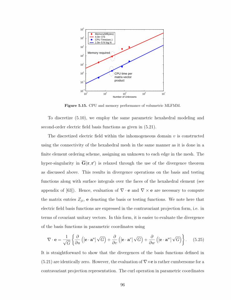
103

104

105

106

107

10−2

10−1

100

101

102

103

104

105

Number of Unknowns

Memory(MBytes)4.0e−3 NCPU Time(sec.)1.0e−5 N log N

Memory required

CPU time permatrix-vectorproduct

Figure 5.15. CPU and memory performance of volumetric MLFMM.

To discretize (5.10), we employ the same parametric hexahedral modeling and

second-order electric field basis functions as given in (5.21).

The discretized electric field within the inhomogeneous domain v is constructed

using the connectivity of the hexahedral mesh in the same manner as it is done in a

finite element ordering scheme, assigning an unknown to each edge in the mesh. The

hyper-singularity in G(r, r′) is relaxed through the use of the divergence theorem

as discussed above. This results in divergence operations on the basis and testing

functions along with surface integrals over the faces of the hexahedral element (see

appendix of [63]). Hence, evaluation of ∇ · e and ∇ × e are necessary to compute

the matrix entries Zji, e denoting the basis or testing functions. We note here that

electric field basis functions are expressed in the contravariant projection form, i.e. in

terms of covariant unitary vectors. In this form, it is easier to evaluate the divergence

of the basis functions in parametric coordinates using

∇ · e =1√G

∂

∂u

([e · au]

√G

)+

∂

∂v

([e · av]

√G

)+

∂

∂w

([e · aw]

√G

). (5.25)

It is straightforward to show that the divergences of the basis functions defined in

(5.21) are identically zero. However, the evaluation of∇×e is rather cumbersome for a

contravariant projection representation. The curl operation in parametric coordinates

96

requires the covariant components of the basis functions, i.e.

∇× e =1√G

[∂ (e · aw)

∂v− ∂ (e · av)

∂w

]au (5.26)

+

[∂ (e · au)

∂w− ∂ (e · aw)

∂u

]av +

[∂ (e · av)

∂u− ∂ (e · au)

∂v

]aw

in which the covariant components must be evaluated using the metric of the para-

metric transformation that forms the curvilinear element as

e · au

e · av

e · aw

=

(au · au) (au · av) (au · aw)

(av · au) (av · av) (av · aw)

(aw · au) (aw · av) (aw · aw)

e · au

e · av

e · aw

. (5.27)

With this substitution, evaluation of (5.26) is rather cumbersome, requiring paramet-

ric derivatives of√

G. As an example, the computation of ∂(e·aw)∂v

for the specific case

when e = 1√G(1− v)(1− w)au gives

∂ (e · aw)

∂v=

∂

∂v[(aw · au)(e · au) + (aw · av)(e · av) + (aw · aw)(e · aw)] (5.28)

=∂

∂v

[(∂r

∂w· ∂r

∂u

) (1√G

(1− v)(1− w)

)]

=

[∂

∂v

(∂r

∂w· ∂r

∂u

)] (1√G

(1− v)(1− w)

)

+

(∂r

∂w· ∂r

∂u

) [∂

∂v

1√G

](1− v)(1− w)− 1√

G

(∂r

∂w· ∂r

∂u

)

Nevertheless, once implemented, the same singularity annihilation method as in [63]

(also see Appendix B) can be used to calculate the resulting matrix elements for the

self-cell terms given by

Zji = 〈ej(r), ei(r)〉 − k20〈ej(r),

∫

vdr′G(r, r′) ·

(εr − I

)· ei(r

′)〉 (5.29)

+ 〈ej(r),∫

vdr′∇′ ×G(r, r′) ·

(µ−1

r − I)· ∇′ × ei(r

′)〉.

The right hand side of the matrix system in the parametric space takes the form

bj = 〈ej(r),Einc(r)〉.

97

Having presented the implementation of the integral equation (5.10) for the vol-

ume fields E, we next proceed to validate this implementation. First, we consider

calculations for purely magnetic materials. Consider the scattering by a permeable

cube (plane wave incidence is normal to the cube’s face). The specific cube has a

side length of 0.5λ0 and µr = 2.2. As seen, the VIE and FE-BI data are in good

agreement and demonstrate the validity of (5.10). Also shown in Fig. 5.16 (b) is the

radar scattering by a spherical shell having an outer radius of 0.2λ0, an inner radius

of 0.18λ0, and a relative permeability of µr = 2.2. Again, the agreement between the

FE-BI and VIE data is excellent.

0 45 95 135 180−30

−25

−20

−15

−10

−5

0

Observation Angle (Degrees)

Bis

tatic

RC

S (

dB/λ

2 )

VIEFEBI

0 45 95 135 180−80

−70

−60

−50

−40

−30

−20

−10

Observation Angle (Degrees)

Bis

tatic

RC

S (

dB/λ

2 )

VIEFEBI

(a) (b)

Figure 5.16. Bistatic RCS of two magnetically permeable scatterers, (a) A cube of side length 0.5λand µr = 2.2, (b) A spherical shell of µr = 2.2, 0.2λ outer radius, and 0.18λ inner radius.

For the validation of the VIE for composite structures, we present scattering

computations from three different configurations. The solution of (5.10) will be com-

pared with corresponding results based on the FE-BI method. Our first example is a

composite cube of side length 0.2λ0. The incident plane wave is propagating in the

negative z direction and the bistatic RCS of the cube is plotted in Fig. 5.17. For

this special case, the covariant and contravariant components of the basis functions

are just scaled versions of each other,√

G is constant, and hence the curl operation

is fairly straightforward to calculate. As seen, the agreement between the VIE and

98

FE-BI solution is very good for both polarizations.

0 45 95 135 180−60

−50

−40

−30

−20

−10

Observation Angle (Degrees)

Bis

tatic

RC

S (

dB/λ

2 )

VIEFEBI

Figure 5.17. Bistatic radar cross section (RCS) of a homogeneous composite cube of side lengtha = 0.2λ, and εr = 1.5, µr = 2.2.

As a second example, we consider a thin spherical shell of outer radius of 0.2λ0,

thickness 0.02λ0 and of the same material parameters (εr = 1.5, µr = 2.2) as in the

previous example. For modelling, the mesh is constructed entirely as a thin layer of

distorted (non-rectangular) curvilinear elements, and both VIE and FE-BI solution

used the same mesh. The bistatic RCS is shown in Fig. 5.18 and it is clear that the

solutions are again in full agreement.

Finally, as our third example, we evaluate the RCS of a solid sphere of radius

0.15λ0. The permittivity and permeability of the sphere are again εr = 1.5 and

µr = 2.2, respectively. We again used the same volumetric mesh as shown in Fig. 5.19

for both methods. Again, excellent agreement is seen between the VIE and FE-BI

solutions.

We note here that, since the same volumetric mesh is used for both the VIE and

FE-BI solutions, and since both the FE-BI volume basis functions and the VIE basis

are functions associated with the edges of the mesh, the resulting number of volumet-

99

0 45 95 135 180−80

−70

−60

−50

−40

−30

−20

−10

Observation Angle (Degrees)

Bis

tatic

RC

S (

dB)

VIEFEBI

Figure 5.18. Bistatic RCS of a composite spherical shell. The outer shell radius is ro = 0.2λ, itsthickness is d = 0.02λ, and its relative constitutive parameters are (εr = 1.5, µr = 2.2).

ric unknowns in both methods are the same. However, the FE-BI method requires

an additional set of surface unknowns since both E and H are solved on the surface s

bounding of the volume v. Hence, the resulting FE-BI system is of higher rank than

the VIE system. Nevertheless, the FE-BI system is partly full and mostly sparse. In

contrast, the VIE system is fully populated and thus requires substantial computation

time for its generation. However, since the VIE is a second kind integral equation,

its iterative solution converges quickly. As an example, for a system of 1082 (second

example) VIE unknowns, the conjugate gradient squared (CGS) solver converged in

5 iterations for a relative error of 10−2 and the solution was completed in only 0.7

seconds using a 1 GHz PIII processor. For the third example (880 VIE unknowns),

the iterative CGS solver converged in 13 iterations and took 1.1 seconds. To our

knowledge, this is the first published implementation of the VIE for inhomogeneous

volumes having both dielectric and magnetic properties.

100

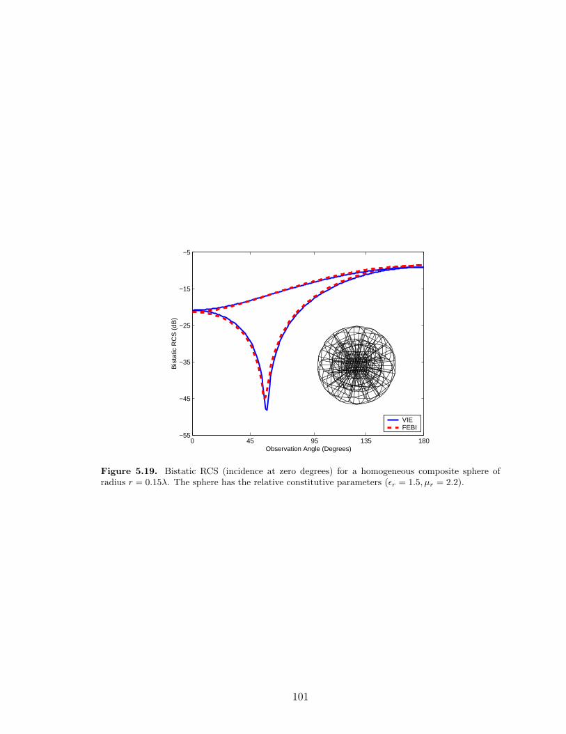
0 45 95 135 180−55

−45

−35

−25

−15

−5

Observation Angle (Degrees)

Bis

tatic

RC

S (

dB)

VIEFEBI

Figure 5.19. Bistatic RCS (incidence at zero degrees) for a homogeneous composite sphere ofradius r = 0.15λ. The sphere has the relative constitutive parameters (εr = 1.5, µr = 2.2).

101

CHAPTER 6

Conclusions

Owing to their lower numerical error and stability, integral equation solution meth-

ods have increasingly become popular over the last five years. Although more costly

than partial differential equation methods, their superior error performance has pro-

vided accurate solutions to electromagnetics problems. Key to the increased utiliza-

tion of integral methods has been the introduction of fast solution procedures such

as the MLFMM.

The fidelity of the mathematical model is also a critical factor in attaining highly

accurate numerical solutions that reflect the actual problem. The contribution of this

thesis has primarily been on the introduction of curvilinear elements for high fidelity

geometry modeling in conjunction with the MLFMM. Also, for the first time, integral

methods were developed and applied to penetrable volumetric structures of arbitrary

composition.

Most methods developed till now dealt with low-order geometry modeling, using

flat-facets or low-order tetrahedra. This approximation introduces numerical error

in the solution process. Also, fine details and large surface curvatures result in very

fine tessellations increasing the computational cost of the solution process. Better

geometry modeling schemes are thus necessary to minimize geometry modeling error.

In the thesis we presented the application of the MLFMM to efficiently solve

surface and volume integral equation using curvilinear geometry modeling. Particular

contributions of the thesis are

102

• MLFMM solution for PEC scattering problems using curvilinear biquadratic

surface modeling.

• MLFMM solutions of hybrid FE-BI systems using curvilinear hexahedral vol-

ume elements.

• Development and numerical solutions of VIEs for modeling inhomogeneous ge-

ometries involving both dielectric and magnetic material parameters.

Also, accuracy and computational savings of the MLFMM were presented and con-

trasted to other solution methods.

To summarize, Chapter 2 outlined a framework for conformal geometry represen-

tation using curvilinear elements for surface modeling. This framework provided a

generalization of flat-facet modeling using low-order elements and forms a basis to

extend various formulations and definitions to higher-order geometry modeling and

higher-order field expansions. We also showed that the size of the resulting system

can be reduced by using curvilinear elements. Hence larger problems can be solved

on the same computing platform.

In addition to using better geometry models to reduce the solution error, we pre-

sented the MLFMM in Chapter 3 for the rapid solution of SIEs and hybrid FE-BI

systems as well as VIEs. This removed the O(N2) computational bottleneck of the

conventional MoM. The accuracy and efficiency of the methods were demonstrated

and ILU preconditioning was employed for better convergence. This is especially

important for the evaluation of multiple incidence angles (e.g. monostatic RCS pre-

dictions) where the same system must be solved many times.

In Chapter 4, we outlined the FE-BI procedure described in [19] and appended it

with the MLFMM. We also gave an extensive presentation of the curvilinear geometry

descriptions for volumetric elements.

As an alternative to the FE-BI method for inhomogeneous targets, a VIE formu-

lation was presented in Chapter 5. Derivation of a new integral equation was given

103

and its implementation using curvilinear volumetric elements and conformal basis

functions of various orders was presented. The numerical solution of such a VIE

for magnetically permeable materials using a reduced number of unknowns and con-

formal geometry modeling is a major contribution of this work. Second-order basis

functions defined in Chapter 5 enabled the solution of the proposed VIE in terms of

only the electric field unknown. Furthermore, the MLFMM was applied to the so-

lution of VIEs for possibly lossy dielectric targets using zeroth-order (parametrically

constant) basis functions that allow for a physical domain decomposition. The accu-

racy and the numerical efficiency of VIE-MLFMM were demonstrated by comparing

the generated results with reference solutions. Implementation issues for MLFMM

on distributed memory computing platforms was presented in Appendix D. Another

appendix presented the important details of the evaluation of the singular kernels

in the VIE. Specifically, an annihilation method that involved a series of parametric

transformations to remove the singularity was presented. Performance and advan-

tages of the annihilation method over the conventional singularity extraction method

were demonstrated for SIE implementations.

Much progress has indeed been achieved in this work for modeling high contrast

penetrable materials. However, greater efficiencies can be achieved by considering

higher-order basis functions with conformal geometrical features. This remains a

future extension of the work. Combination of different elements is also advantageous

in modeling geometry details.

For a multi-spectral analysis, the methods presented in this thesis must be em-

ployed repeatedly for each frequency. Depending on the electrical size of the problem,

each solution may require considerable amount of CPU time and memory. However,

significant speed-ups can be achieved by using the previous frequency solution in-

formation. Similarly, for a single frequency, the matrix system needs to be solved

repeatedly for different excitations. In this case, block solvers may be utilized to

104

concurrently solve for multiple right hand sides.

Although the complexity of the MLFMM is low, the implementation will have an

upper limit on the size of the largest problem to be analyzed. To solve even larger

problems, one has to resort to using high-frequency approximations such as the PO or

the geometrical theory of diffraction. Hybridization of MLFMM with high-frequency

methods is an area that deserves serious investigation and a significant investment.

Although the thesis did not focus on applications, the presented methods have

a wide range of applicability. RCS and antenna analysis are certainly the most

direct applications. However, the developed algorithms have great applicability to

bio-medical imaging, indoor propagation in wireless systems, EMI/EMC for aircraft

and radio frequency (RF) circuits. Moreover, the speed-up offered opens for the first

time possibilities for designing RF devices and possibly complete RF systems.

105

APPENDICES

106

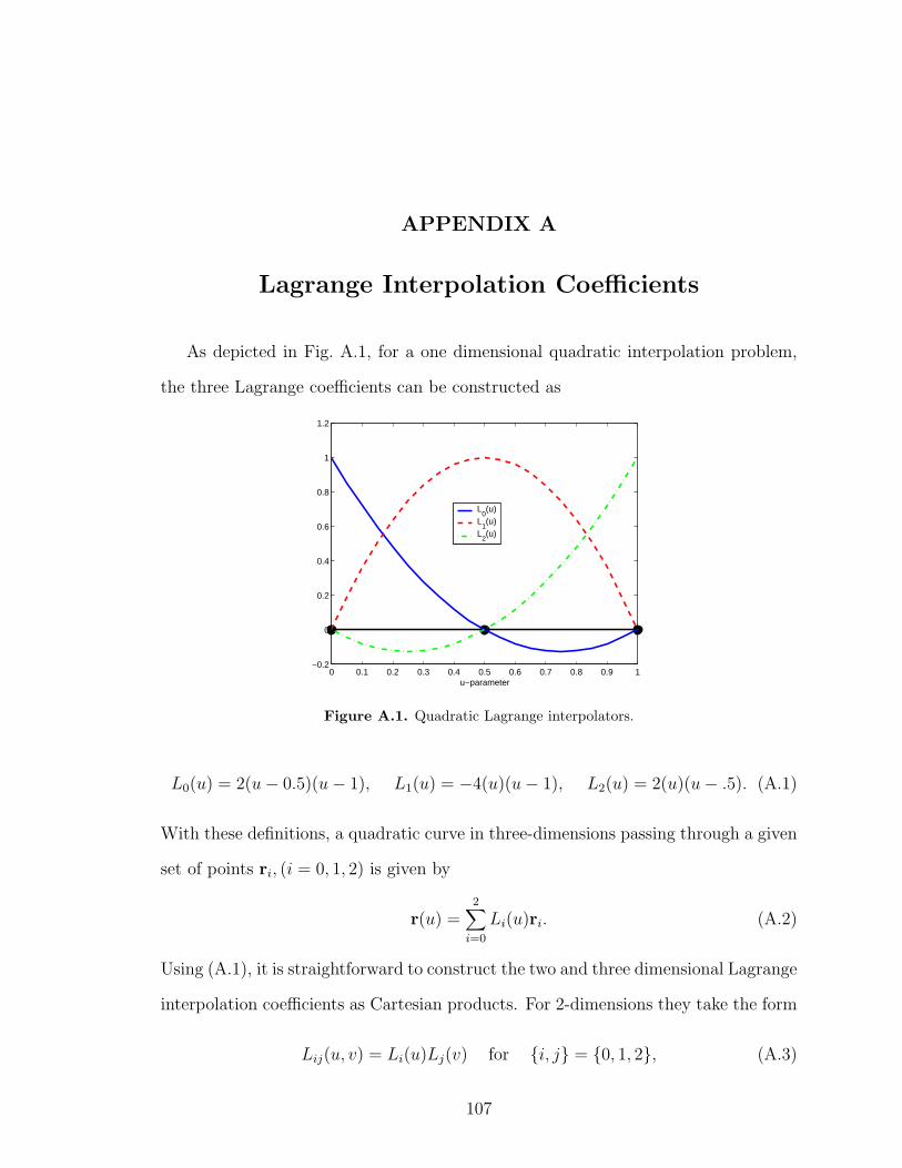
APPENDIX A

Lagrange Interpolation Coefficients

As depicted in Fig. A.1, for a one dimensional quadratic interpolation problem,

the three Lagrange coefficients can be constructed as

0 0.1 0.2 0.3 0.4 0.5 0.6 0.7 0.8 0.9 1−0.2

0

0.2

0.4

0.6

0.8

1

1.2

u−parameter

L0(u)

L1(u)

L2(u)

Figure A.1. Quadratic Lagrange interpolators.

L0(u) = 2(u− 0.5)(u− 1), L1(u) = −4(u)(u− 1), L2(u) = 2(u)(u− .5). (A.1)

With these definitions, a quadratic curve in three-dimensions passing through a given

set of points ri, (i = 0, 1, 2) is given by

r(u) =2∑

i=0

Li(u)ri. (A.2)

Using (A.1), it is straightforward to construct the two and three dimensional Lagrange

interpolation coefficients as Cartesian products. For 2-dimensions they take the form

Lij(u, v) = Li(u)Lj(v) for i, j = 0, 1, 2, (A.3)

107

and a biquadratic surface patch defined by 9 points in space (rij, i, j = 0, 1, 2)on a topologically rectangular grid is given by

r(u, v) =2∑

i=0

2∑

j=0

Lij(u, v)rij. (A.4)

Similarly, for 3-dimensions the Lagrange interpolators are constructed as

Lijk(u, v, w) = Li(u)Lj(v)Lk(w) for i, j, k = 0, 1, 2, (A.5)

and for the tri-quadratic hexahedral element

r(u, v, w) =2∑

i=0

2∑

j=0

2∑

k=0

Lijk(u, v, w)rijk (A.6)

where rijk, i, j, k = 0, 1, 2 are the 27 defining points.

108

APPENDIX B

Singularity Annihilation Methods for Surfaces and

Volumes

The matrix elements in (5.29) can be rewritten as

Zji = 〈ej(r), ei(r)〉 − 〈ej(r), I1(r)〉 − 1

k20

〈ej(r), I2(r)〉, (B.1)

where

I1(r) =∫

vdv′g(r, r′)(k2(r′)− k2

0)ei(r′) (B.2)

and

I2(r) = ∇∫

vdv′∇g(r, r′) · (k2(r′)− k2

0)ei(r′). (B.3)

To deal with the 1/ |r− r′|3 singularity in I2(r) we proceed as usual by transferring

the ∇ operator onto the testing function. We have,

∫

vdvej(r) · I2(r) =

∫

vdvej(r) · ∇

∫

vdv′∇g(r, r′) · (k2(r′)− k2

0)ei(r′)

=∫

vdv∇ ·

[ej(r)

∫

vdv′∇g(r, r′) · (k2(r′)− k2

0)ei(r′)

]

−∫

vdv [∇ · ej(r)]

∫

vdv′∇g(r, r′) · (k2(r′)− k2

0)ei(r′)

=∮

sds ·

[ej(r)

∫

vdv′∇g(r, r′) · (k2(r′)− k2

0)ei(r′)

]

−∫

vdv∇ · ej(r)

∫

vdv′∇g(r, r′) · (k2(r′)− k2

0)ei(r′), (B.4)

109

where s denotes the surface enclosing v. The source (primed) integral in (B.4) can

further be rewritten as

∫

vdv′∇g(r, r′) · (k2(r′)− k2

0)ei(r′) = −

∫

vdv′∇′g(r, r′) · (k2(r′)− k2

0)ei(r′)

= −∫

vdv′∇′ ·

[g(r, r′) · (k2(r′)− k2

0)ei(r′)

]

+∫

vdv′g(r, r′)∇′ ·

[(k2(r′)− k2

0)ei(r′)

]

= −∮

sds′ · g(r, r′)(k2(r′)− k2

0)ei(r′)

+∫

vdv′g(r, r′)∇′ ·

[(k2(r′)− k2

0)ei(r′)

](B.5)

The above integrals are not improper, nevertheless, their numerical integration

must be carefully done due to the first order singularity of the Green’s function. To

evaluate the singular source integrals in (B.5), we herewith employ an annihilation

technique that converts the singular integrands from the original (u, v, w) parametric

space to smooth, non-singular integrands on an auxiliary (α, β, γ) parametric space.

To illustrate this, let us consider the volume integral in (B.5) involving the divergence

of the basis functions. First, we recast it in the (u, v, w) space as

I =∫ 1

0

∫ 1

0

∫ 1

0g(r, r′)∇′ ·

[(k2(r′)− k2

0)ei(r′)

]√Gdudvdw. (B.6)

For further discussion, we conveniently rewrite (B.6) in a more general form as a ratio

of two well behaved functions in the (u, v, w) space

I =∫ 1

0

∫ 1

0

∫ 1

0

f(u0, v0, w0, u, v, w)

g(u0, v0, w0, u, v, w)dudvdw (B.7)

where g(u0, v0, w0, u, v, w) = 0 when (u, v, w) = (u0, v0, w0) and f(u0, v0, w0, u, v, w)

is well behaved at the same point. We note that in (B.7), the original observation

point has been mapped to (u0, v0, w0).

The next step in the annihilation process is to divide the unit cube into eight

quadrants using the three isoparametric planes defined by u = u0, v = v0, and

w = w0 (see Fig. B.1 (a)). When these quadrants are considered separately, the

110

original singularity now appears at a vertex of each of the eight quadrants. For

integration, we next proceed to map each of the eight quadrants to a unit cube in

the (η, ζ, ξ) parametric space as shown in Fig. B.1 (b). We need to again be careful

to choose our transformations so that the singularity for one of the vertices of each

quadrant appears at the origin of the (η, ζ, ξ) space. For example, the transformation

to map the quadrant defined by (u0 < u < 1), (0 < v < v0), (w0 < w < 1) is

u = (1− u0)η + u0

v = v0(1− ζ)

w = (1− w0)ξ + w0. (B.8)

Similar transformations must be used for the other seven quadrants.

Using this eight-quadrant decompositions, the integral (B.7) can be written as

I =8∑

i=1

∫ 1

0

∫ 1

0

∫ 1

0

fi(η, ζ, ξ)

gi(η, ζ, ξ)Ji(η, ζ, ξ)dηdζdξ (B.9)

where Ji(η, ζ, ξ) are the Jacobians of the transformations for each quadrant and fi

and gi are the portions of the original f and g that fall in respective quadrants. We

should remark that fi, gi, and Ji do depend on (u0, v0, w0), but this dependence has

been suppressed. Also, since the transformations used to map (η, ζ, ξ) to (u, v, w)

are simple scaling transformations, the Jacobians Ji(η, ζ, ξ) are constants. For the

example given in (B.8), the Jacobian is simply Ji = (1− u0)(−v0)(1− w0).

A final step for integration is to propose another parametric transformation whose

Jacobian has a zero (of order equal to or higher than that of g) at the origin of the

(η, ζ, ξ) space (Fig. B.1 (c)). One such transformation is

η = α3

ζ = β3

ξ = γ3 (B.10)

111

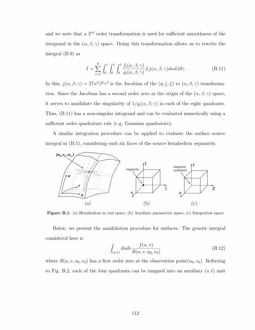
and we note that a 3rd order transformation is used for sufficient smoothness of the

integrand in the (α, β, γ) space. Doing this transformation allows us to rewrite the

integral (B.9) as

I =8∑

i=1

∫ 1

0

∫ 1

0

∫ 1

0

fi(α, β, γ)

gi(α, β, γ)Jij(α, β, γ)dαdβdγ (B.11)

In this, j(α, β, γ) = 27α2β2γ2 is the Jacobian of the (η, ζ, ξ) to (α, β, γ) transforma-

tion. Since the Jacobian has a second order zero at the origin of the (α, β, γ) space,

it serves to annihilate the singularity of 1/gi(α, β, γ) in each of the eight quadrants.

Thus, (B.11) has a non-singular integrand and can be evaluated numerically using a

sufficient order quadrature rule (e.g. Gaussian quadrature).

A similar integration procedure can be applied to evaluate the surface source

integral in (B.5), considering each six faces of the source hexahedron separately.

u

v

w

(u ,v ,w )0 0 0

ηζ

ξsingularity

αβ

γsingularity annihilated

(a) (b) (c)

Figure B.1. (a) Hexahedron in real space, (b) Auxiliary parametric space, (c) Integration space

Below, we present the annihilation procedure for surfaces. The generic integral

considered here is∫

(u,v)dudv

f(u, v)

R(u, v, u0, v0)(B.12)

where R(u, v, u0, v0) has a first order zero at the observation point(u0, v0). Referring

to Fig. B.2, each of the four quadrants can be mapped into an auxiliary (s, t) unit

112

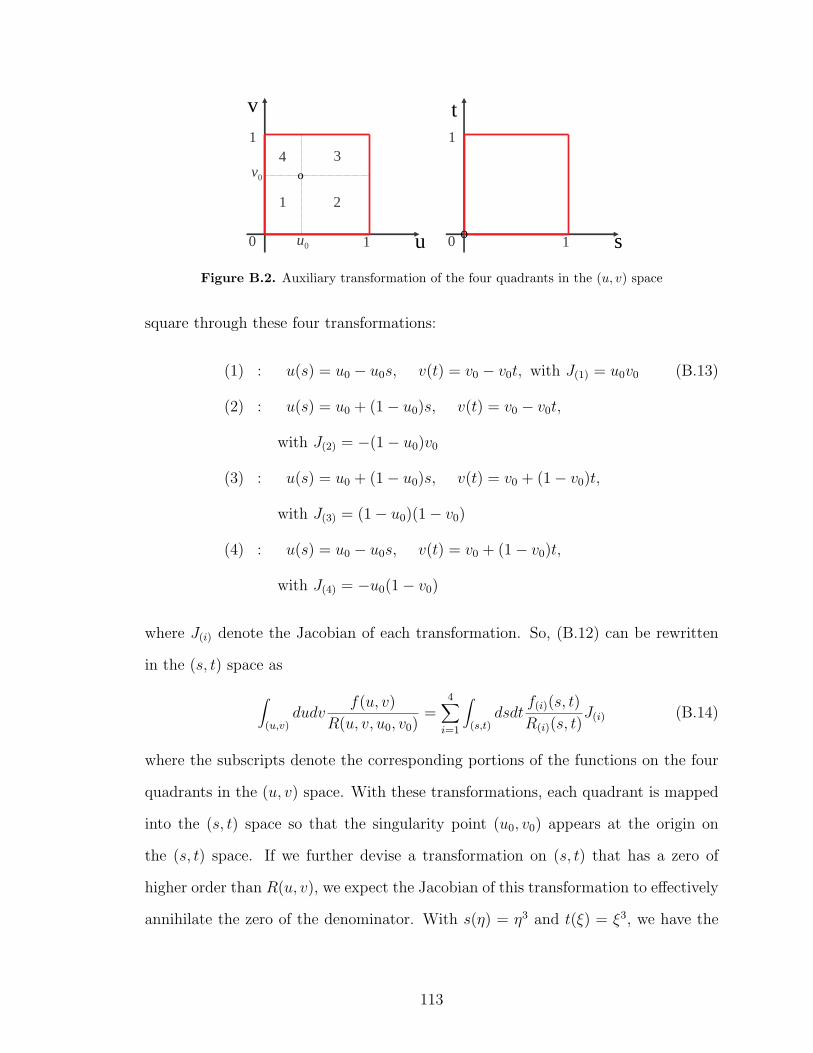
1

1

0 so

t

1

1

0

0v

0u u

1

4 3

2

o

v

Figure B.2. Auxiliary transformation of the four quadrants in the (u, v) space

square through these four transformations:

(1) : u(s) = u0 − u0s, v(t) = v0 − v0t, with J(1) = u0v0 (B.13)

(2) : u(s) = u0 + (1− u0)s, v(t) = v0 − v0t,

with J(2) = −(1− u0)v0

(3) : u(s) = u0 + (1− u0)s, v(t) = v0 + (1− v0)t,

with J(3) = (1− u0)(1− v0)

(4) : u(s) = u0 − u0s, v(t) = v0 + (1− v0)t,

with J(4) = −u0(1− v0)

where J(i) denote the Jacobian of each transformation. So, (B.12) can be rewritten

in the (s, t) space as

∫

(u,v)dudv

f(u, v)

R(u, v, u0, v0)=

4∑

i=1

∫

(s,t)dsdt

f(i)(s, t)

R(i)(s, t)J(i) (B.14)

where the subscripts denote the corresponding portions of the functions on the four

quadrants in the (u, v) space. With these transformations, each quadrant is mapped

into the (s, t) space so that the singularity point (u0, v0) appears at the origin on

the (s, t) space. If we further devise a transformation on (s, t) that has a zero of

higher order than R(u, v), we expect the Jacobian of this transformation to effectively

annihilate the zero of the denominator. With s(η) = η3 and t(ξ) = ξ3, we have the

113

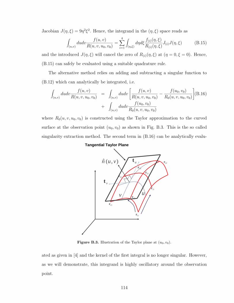
Jacobian J(η, ξ) = 9η2ξ2. Hence, the integrand in the (η, ξ) space reads as

∫

(u,v)dudv

f(u, v)

R(u, v, u0, v0)=

4∑

i=1

∫

(η,ξ)dηdξ

f(i)(η, ξ)

R(i)(η, ξ)J(i)J(η, ξ) (B.15)

and the introduced J(η, ξ) will cancel the zero of R(i)(η, ξ) at (η = 0, ξ = 0). Hence,

(B.15) can safely be evaluated using a suitable quadrature rule.

The alternative method relies on adding and subtracting a singular function to

(B.12) which can analytically be integrated, i.e.

∫

(u,v)dudv

f(u, v)

R(u, v, u0, v0)=

∫

(u,v)dudv

[f(u, v)

R(u, v, u0, v0)− f(u0, v0)

R0(u, v, u0, v0)

](B.16)

+∫

(u,v)dudv

f(u0, v0)

R0(u, v, u0, v0)

where R0(u, v, u0, v0) is constructed using the Taylor approximation to the curved

surface at the observation point (u0, v0) as shown in Fig. B.3. This is the so called

singularity extraction method. The second term in (B.16) can be analytically evalu-

21r

22r

32r

32r

33r

11r

12r

13r

uv

ut

vt

),(ˆ vun

Tangential Taylor Plane

Figure B.3. Illustration of the Taylor plane at (u0, v0).

ated as given in [4] and the kernel of the first integral is no longer singular. However,

as we will demonstrate, this integrand is highly oscillatory around the observation

point.

114

We consider three cases as shown in Fig. B.4 with three different integration

domains having increasing curvatures. The numerical integral of (B.12) using Gaus-

sian quadrature is given in Fig. B.4. The error is evaluated with respect to a 50

point Gaussian quadrature using the annihilation method. As seen in this figure, the

annihilation method provides almost a monotonic convergence as compared to the

extraction method. As the element curvature gets larger, the annihilation method

fails to accurately integrate (B.12). The reason behind this behavior can be found

when we look at the actual integrands of both methods. Shown in Fig. B.5 are the

integrands that are numerically evaluated for the three cases. For the annihilation

method, the integrands are plotted in the (η, ξ) space where there is no singular-

ity. On the other hand, we can obviously observe that an attempt to numerically

evaluate the kernels of the extraction method will be problematic due to high os-

cillations around the observation point. Even though the kernels are not singular,

rapid changes around (u0, v0) will render a numerical integration scheme based on

polynomial approximations of the kernel useless.

115

Case I , Slight curvature

0 5 10 15 20 25 30-8

-7

-6

-5

-4

-3

-2

-1

0

1

Number of Gaussian Integration Points in each Parametric Dimension

Log

of e

rror

Integration of 1/R Singularity on Curved Patches

AnnihilationExtraction

u0 = 0.4, v0 = 0.7

Log of error in the integral

0 5 10 15 20 25 30-7

-6

-5

-4

-3

-2

-1

0

1

Number of Gaussian Integration Points in each Parametric Dimension

Log

of e

rror

Integration of 1/R Singularity on Curved Patches

AnnihilationExtraction

Case II , Medium curvatureu0 = 0.6, v0 = 0.2

0 5 10 15 20 25 30-7

-6

-5

-4

-3

-2

-1

0

Number of Gaussian Integration Points in each Parametric Dimension

Log

of e

rror

Integration of 1/R Singularity on Curved Patches

AnnihilationExtraction

Case III, High curvatureu0 = 0.1, v0 = 0.3

Log of error in the integral

Log of error in the integral

Figure B.4. Performances of annihilation and extraction methods for three different cases.

116

Case I Case II Case III

Annihilation Annihilation Annihilation

Extraction Extraction Extraction

Figure B.5. Kernels of both methods for the three cases.

117

APPENDIX C

Incomplete LU Preconditioner for FMM

implementation

For large scale simulations, possibly with geometrical surface details (e.g. antenna

arrays on aircraft), the density of the surface mesh cannot be expected to be uni-

form. Nevertheless, a nonuniform mesh is well known to produce ill-conditioned MoM

matrix equations. Also, different formulations of the same electromagnetic problem

are associated with different condition numbers. For example, the CFIE formulation

is known to give rise to much better conditioned systems than the EFIE or MFIE.

Further, as noted above, the FMM implementation introduces erroneous minima in

the solution domain. Use of a preconditioner is therefore essential for robust imple-

mentations of iterative solvers.

Although the diagonal preconditioner is simple and leads to significant conver-

gence improvements, it does so for diagonally dominant matrices. Block diagonal

preconditioners are more robust but require renumbering of the grid or matrix rear-

ranging so that the dominant matrix terms are clustered around the diagonal. This

can easily be done for 2D problems, but is quite difficult, if at all possible, in three

dimensions. Alternatively, when the FMM is used to speed up the iterative solution,

we have the natural choice of using the near-field portion of the MoM matrix for pre-

conditioning. These near-field elements are the largest in magnitude and constitute

the un-approximated portion of the system matrix.

One preconditioning approach is to perform a direct LU decomposition on the

un-approximated part of the matrix. However, depending on the sparsity pattern of

118

the near-field matrix, this may require a significant amount of fill-ins. For large scale

simulations, these fill-ins may become a bottleneck in memory utilization. Alterna-

tively, the fill-in requirement of direct LU can be resolved by performing the ILU

factorization. The ILU is the same as a direct LU algorithm but avoids fill-ins of

elements in the decomposed LU matrices. This also results in less CPU utilization.

The ILU algorithm from [39] has been incorporated into the FMM solver. The

pseudo code is repeated below for completeness.

for i = 2,...,n, do:

for k = 1,...,i-1 and for (i,k) in NZ(Z) do:

compute zik = zik/zkk

for j = k+1,...,n and for (i,j) in NZ(Z) do:

compute zij = zij − zikzkj

end do

end do

end do

Here NZ(Z) is the sparsity pattern of the near-field matrix Z, and the conventional

LU decomposition algorithm is only applied to the non-zero entries of the matrix.

Hence, memory utilization is not affected and moreover the sparsity pattern of the

stored ILU matrix is identical to that of the original matrix. Thus, further memory

savings are attained using ILU decomposition.

C.1 ILU Performance

To evaluate the performance of the ILU preconditioner, we considered a perfectly

electrically conducting (PEC) ogive geometry (depicted in Fig. 2.10 (f)). For this

study, the ILU preconditioner was implemented in the matrix systems based on the

119

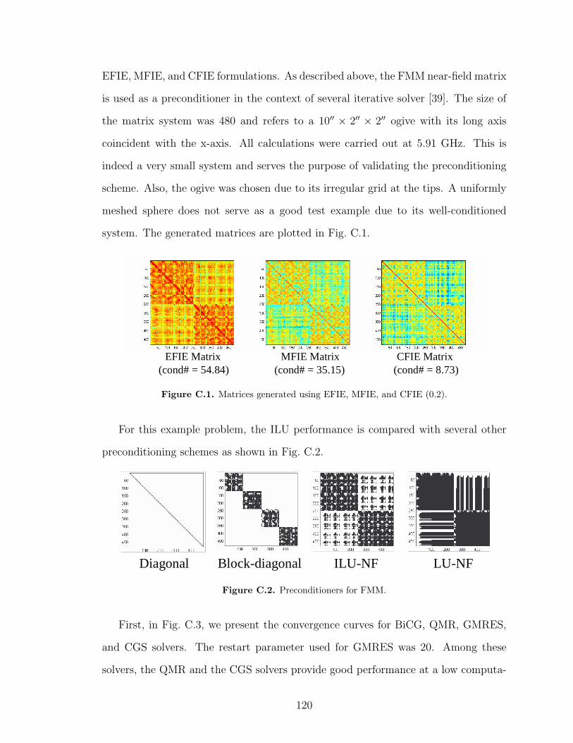
EFIE, MFIE, and CFIE formulations. As described above, the FMM near-field matrix

is used as a preconditioner in the context of several iterative solver [39]. The size of

the matrix system was 480 and refers to a 10′′ × 2′′ × 2′′ ogive with its long axis

coincident with the x-axis. All calculations were carried out at 5.91 GHz. This is

indeed a very small system and serves the purpose of validating the preconditioning

scheme. Also, the ogive was chosen due to its irregular grid at the tips. A uniformly

meshed sphere does not serve as a good test example due to its well-conditioned

system. The generated matrices are plotted in Fig. C.1.

EFIE Matrix MFIE Matrix CFIE Matrix(cond# = 54.84) (cond# = 35.15) (cond# = 8.73)

Figure C.1. Matrices generated using EFIE, MFIE, and CFIE (0.2).

For this example problem, the ILU performance is compared with several other

preconditioning schemes as shown in Fig. C.2.

Diagonal Block-diagonal LU-NFILU-NF

Figure C.2. Preconditioners for FMM.

First, in Fig. C.3, we present the convergence curves for BiCG, QMR, GMRES,

and CGS solvers. The restart parameter used for GMRES was 20. Among these

solvers, the QMR and the CGS solvers provide good performance at a low computa-

120

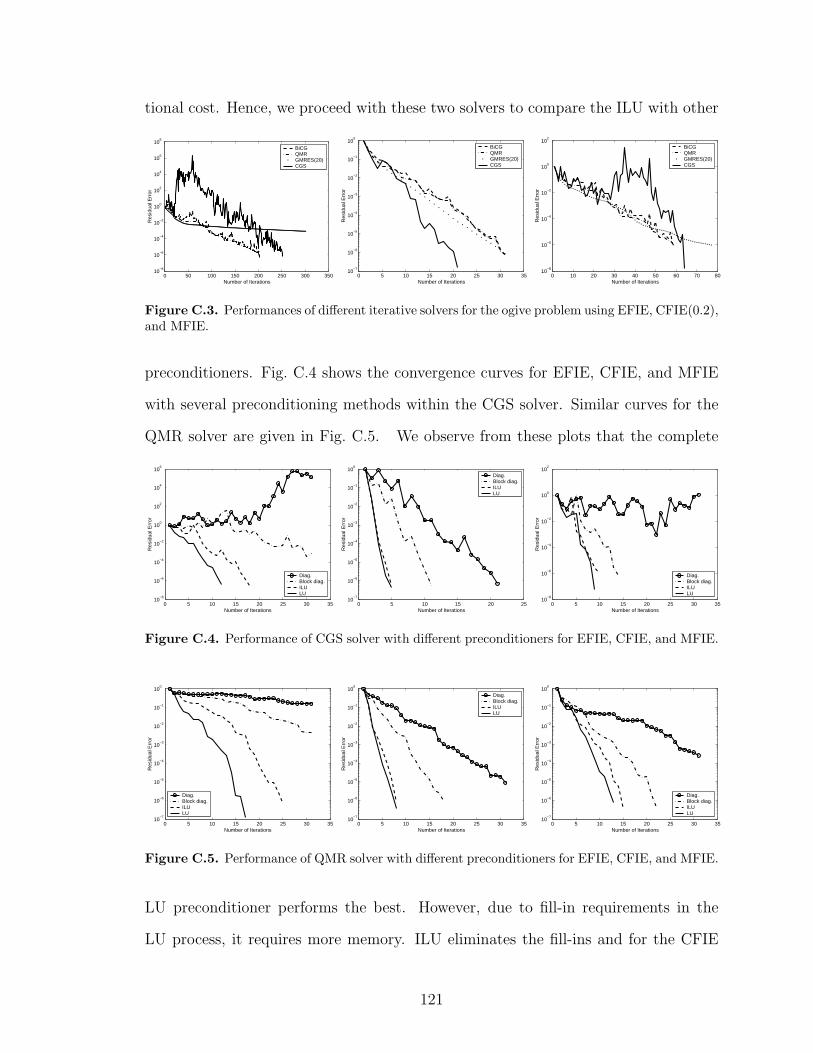
tional cost. Hence, we proceed with these two solvers to compare the ILU with other

0 50 100 150 200 250 300 35010

−8

10−6

10−4

10−2

100

102

104

106

108

Number of Iterations

Res

idua

l Err

orBiCGQMRGMRES(20)CGS

0 5 10 15 20 25 30 3510

−7

10−6

10−5

10−4

10−3

10−2

10−1

100

Number of Iterations

Res

idua

l Err

or

BiCGQMRGMRES(20)CGS

0 10 20 30 40 50 60 70 8010

−8

10−6

10−4

10−2

100

102

Number of Iterations

Res

idua

l Err

or

BiCGQMRGMRES(20)CGS

Figure C.3. Performances of different iterative solvers for the ogive problem using EFIE, CFIE(0.2),and MFIE.

preconditioners. Fig. C.4 shows the convergence curves for EFIE, CFIE, and MFIE

with several preconditioning methods within the CGS solver. Similar curves for the

QMR solver are given in Fig. C.5. We observe from these plots that the complete

0 5 10 15 20 25 30 3510

−8

10−6

10−4

10−2

100

102

104

106

Number of Iterations

Res

idua

l Err

or

Diag.Block diag.ILULU

0 5 10 15 20 2510

−7

10−6

10−5

10−4

10−3

10−2

10−1

100

Number of Iterations

Res

idua

l Err

or

Diag.Block diag.ILULU

0 5 10 15 20 25 30 3510

−8

10−6

10−4

10−2

100

102

Number of Iterations

Res

idua

l Err

or

Diag.Block diag.ILULU

Figure C.4. Performance of CGS solver with different preconditioners for EFIE, CFIE, and MFIE.

0 5 10 15 20 25 30 3510

−7

10−6

10−5

10−4

10−3

10−2

10−1

100

Number of Iterations

Res

idua

l Err

or

Diag.Block diag.ILULU

0 5 10 15 20 25 30 3510

−7

10−6

10−5

10−4

10−3

10−2

10−1

100

Number of Iterations

Res

idua

l Err

or

Diag.Block diag.ILULU

0 5 10 15 20 25 30 3510

−7

10−6

10−5

10−4

10−3

10−2

10−1

100

Number of Iterations

Res

idua

l Err

or

Diag.Block diag.ILULU

Figure C.5. Performance of QMR solver with different preconditioners for EFIE, CFIE, and MFIE.

LU preconditioner performs the best. However, due to fill-in requirements in the

LU process, it requires more memory. ILU eliminates the fill-ins and for the CFIE

121

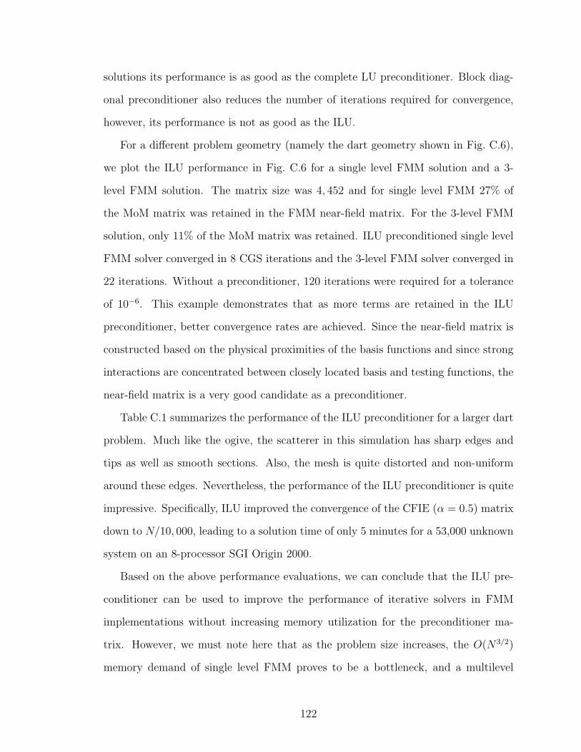
solutions its performance is as good as the complete LU preconditioner. Block diag-

onal preconditioner also reduces the number of iterations required for convergence,

however, its performance is not as good as the ILU.

For a different problem geometry (namely the dart geometry shown in Fig. C.6),

we plot the ILU performance in Fig. C.6 for a single level FMM solution and a 3-

level FMM solution. The matrix size was 4, 452 and for single level FMM 27% of

the MoM matrix was retained in the FMM near-field matrix. For the 3-level FMM

solution, only 11% of the MoM matrix was retained. ILU preconditioned single level

FMM solver converged in 8 CGS iterations and the 3-level FMM solver converged in

22 iterations. Without a preconditioner, 120 iterations were required for a tolerance

of 10−6. This example demonstrates that as more terms are retained in the ILU

preconditioner, better convergence rates are achieved. Since the near-field matrix is

constructed based on the physical proximities of the basis functions and since strong

interactions are concentrated between closely located basis and testing functions, the

near-field matrix is a very good candidate as a preconditioner.

Table C.1 summarizes the performance of the ILU preconditioner for a larger dart

problem. Much like the ogive, the scatterer in this simulation has sharp edges and

tips as well as smooth sections. Also, the mesh is quite distorted and non-uniform

around these edges. Nevertheless, the performance of the ILU preconditioner is quite

impressive. Specifically, ILU improved the convergence of the CFIE (α = 0.5) matrix

down to N/10, 000, leading to a solution time of only 5 minutes for a 53,000 unknown

system on an 8-processor SGI Origin 2000.

Based on the above performance evaluations, we can conclude that the ILU pre-

conditioner can be used to improve the performance of iterative solvers in FMM

implementations without increasing memory utilization for the preconditioner ma-

trix. However, we must note here that as the problem size increases, the O(N3/2)

memory demand of single level FMM proves to be a bottleneck, and a multilevel

122

0 20 40 60 80 100 120 14010

−8

10−6

10−4

10−2

100

102

Convergence of CGS Solver

Residual Error

Num

ber

of It

erat

ions

No PCILU−FMM

1ILU−FMM

3

Figure C.6. Performance of CGS solver with CFIE(0.2) for dart geometry.

FMM implementation becomes necessary. Moreover, for a multilevel implementa-

tion, the size of the near-field matrix decreases, approaching to an almost diagonal

system (with non-zero entries being only of O(N)). Hence, most of the non-zero en-

tries in the near-field matrix of a single level FMM method are lost in the multilevel

implementation. Consequently, this degrades the performance of the ILU precondi-

tioner for the MLFMM case (as predicted by Fig. C.6). Hence, for the MLFMM

implementation, we do not employ any kind of preconditioning.

Number Matrix Precond. Number Residual Timeof Fill LU of Error per

Unknowns Time(min.) Time(min.) Iter. Solution(min.)(8 proc.) (1 proc.) (8 proc.)

53000 77 81 5 0.001 5

Table C.1. Performance of ILU for a large-scale complex target with sharp edges and tips on an8-processor SGI Origin 2000.

123

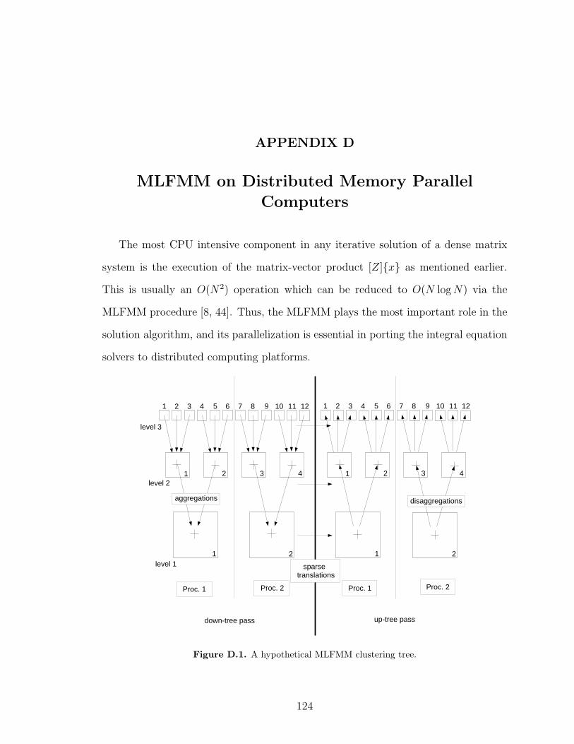
APPENDIX D

MLFMM on Distributed Memory Parallel

Computers

The most CPU intensive component in any iterative solution of a dense matrix

system is the execution of the matrix-vector product [Z]x as mentioned earlier.

This is usually an O(N2) operation which can be reduced to O(N log N) via the

MLFMM procedure [8, 44]. Thus, the MLFMM plays the most important role in the

solution algorithm, and its parallelization is essential in porting the integral equation

solvers to distributed computing platforms.

level 1

level 2

level 3

Proc. 1 Proc. 2 Proc. 1 Proc. 2

disaggregations

sparsetranslations

aggregations

1 2 3 4 1 2 3 4

1 2 3 4 5 6 7 8 9 10 11 12 1 2 3 4 5 6 7 8 9 10 11 12

1 2 1 2

down-tree pass up-tree pass

Figure D.1. A hypothetical MLFMM clustering tree.

124

In considering the parallelization of the matrix-vector products in the MLFMM

algorithm, we must examine the three basic steps within the algorithm. First, the

radiation or signature functions of each group at the (l + 1)th level are aggregated

to form the radiation functions of the parent groups, i.e. groups at the (l)th level.

Secondly, the translation of the radiation functions to cluster centers located in the

far-zone of the source cluster at the (l)th level, provided their parents at the (l− 1)th

level are in the near-zone of each other. The last step is the disaggregation step,

where the children clusters at the (l + 1)th level are disaggregated to compute the

fields within the clusters. These three steps are depicted in Fig. D.1 for a three-level

FMM tree. A successful parallel implementation of these three steps requires

• Careful balancing of the computational load among the processors, and

• Minimal communication between the processors.

Load balancing requires the distribution of the MLFMM tree structure on the nodes

of the parallel process. For the sake of simplicity, let us consider the tree structure

given in Fig. D.1, consisting of 2 main clusters at the coarsest level. If the tree is dis-

tributed on 2 nodes of a parallel process, assuming that each cluster at each level has

the same number of far-zone clusters, we would achieve a perfectly balanced distribu-

tion. For such a case, the aggregation and disaggregation steps can be carried out on

separate processors independently, without inter-processor communication. The only

required communication will take place at the translation step when the source and

target clusters lie on different processors. However, this requires a significant amount

of communication between processors, as will be explained below. With vector pro-

cessing capabilities on computing platforms, the actual work at the translation step

on each processor is quite small and comparable to the time used for communication.

Consequently, communication among processors becomes a bottleneck for the parallel

performance of the MLFMM implementation.

To better explain the situation, let us assume that at the 1st level, clusters 1

125

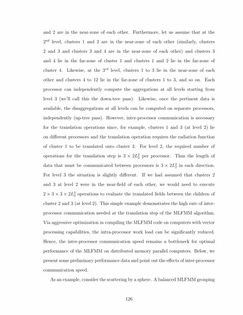
and 2 are in the near-zone of each other. Furthermore, let us assume that at the

2nd level, clusters 1 and 2 are in the near-zone of each other (similarly, clusters

2 and 3 and clusters 3 and 4 are in the near-zone of each other) and clusters 3

and 4 lie in the far-zone of cluster 1 and clusters 1 and 2 lie in the far-zone of

cluster 4. Likewise, at the 3rd level, clusters 1 to 3 lie in the near-zone of each

other and clusters 4 to 12 lie in the far-zone of clusters 1 to 3, and so on. Each

processor can independently compute the aggregations at all levels starting from

level 3 (we’ll call this the down-tree pass). Likewise, once the pertinent data is

available, the disaggregations at all levels can be computed on separate processors,

independently (up-tree pass). However, inter-processor communication is necessary

for the translation operations since, for example, clusters 1 and 3 (at level 2) lie

on different processors and the translation operation requires the radiation function

of cluster 1 to be translated onto cluster 3. For level 2, the required number of

operations for the translation step is 3 × 2L22 per processor. Thus the length of

data that must be communicated between processors is 3 × 2L22 in each direction.

For level 3 the situation is slightly different. If we had assumed that clusters 2

and 3 at level 2 were in the near-field of each other, we would need to execute

2 × 3 × 3 × 2L23 operations to evaluate the translated fields between the children of

cluster 2 and 3 (at level 2). This simple example demonstrates the high rate of inter-

processor communication needed at the translation step of the MLFMM algorithm.

Via aggressive optimization in compiling the MLFMM code on computers with vector

processing capabilities, the intra-processor work load can be significantly reduced.

Hence, the inter-processor communication speed remains a bottleneck for optimal

performance of the MLFMM on distributed memory parallel computers. Below, we

present some preliminary performance data and point out the effects of inter-processor

communication speed.

As an example, consider the scattering by a sphere. A balanced MLFMM grouping

126

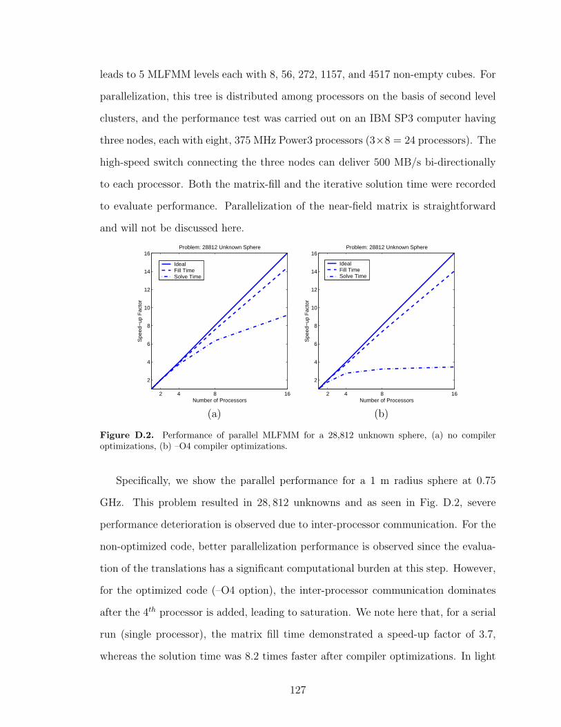
leads to 5 MLFMM levels each with 8, 56, 272, 1157, and 4517 non-empty cubes. For

parallelization, this tree is distributed among processors on the basis of second level

clusters, and the performance test was carried out on an IBM SP3 computer having

three nodes, each with eight, 375 MHz Power3 processors (3×8 = 24 processors). The

high-speed switch connecting the three nodes can deliver 500 MB/s bi-directionally

to each processor. Both the matrix-fill and the iterative solution time were recorded

to evaluate performance. Parallelization of the near-field matrix is straightforward

and will not be discussed here.

2 4 8 16

2

4

6

8

10

12

14

16Problem: 28812 Unknown Sphere

Number of Processors

Spe

ed−

up F

acto

r

IdealFill TimeSolve Time

2 4 8 16

2

4

6

8

10

12

14

16Problem: 28812 Unknown Sphere

Number of Processors

Spe

ed−

up F

acto

r

IdealFill TimeSolve Time

(a) (b)

Figure D.2. Performance of parallel MLFMM for a 28,812 unknown sphere, (a) no compileroptimizations, (b) –O4 compiler optimizations.

Specifically, we show the parallel performance for a 1 m radius sphere at 0.75

GHz. This problem resulted in 28, 812 unknowns and as seen in Fig. D.2, severe

performance deterioration is observed due to inter-processor communication. For the

non-optimized code, better parallelization performance is observed since the evalua-

tion of the translations has a significant computational burden at this step. However,

for the optimized code (–O4 option), the inter-processor communication dominates

after the 4th processor is added, leading to saturation. We note here that, for a serial

run (single processor), the matrix fill time demonstrated a speed-up factor of 3.7,

whereas the solution time was 8.2 times faster after compiler optimizations. In light

127

of the above observations, we conclude that even for a very well balanced problem,

inter-processor communication remains the bottleneck for the parallel performance

of MLFMM on distributed memory computers. Consequently, future efforts must fo-

cus on significant re-organization of the MLFMM algorithm for massively distributed

platforms. One alternative is to distribute the k-space samples among the proces-

sors rather than distributing the basis functions themselves. Since the translation

operation is a diagonal operation, meaning every outgoing plane-wave amplitude is

translated over the testing domain to form the incoming plane-wave amplitude in-

dependent of the rest of the plane-wave directions. This will eliminate any commu-

nication between processors at the translation stage, however, a new interpolation

scheme is necessary since not all of the plane-wave directions will be available on

each processor at a given level.

128

BIBLIOGRAPHY

129

BIBLIOGRAPHY

[1] J.-M. Jin, J. L. Volakis, and V. V. Liepa, “A moment method solution of a

volume-surface integral equation using isoparametric elements and point match-

ing (TE scattering)”, IEEE Trans. Microwave Theory Tech., vol. 37, no. 10, pp.

1641–1645, Oct. 1989.

[2] S. M. Rao, D. R. Wilton, and A. W. Glisson, “Electromagnetic scattering by

surfaces of arbitrary shape”, IEEE Trans. Antennas Propagat., vol. 30, no. 3,

pp. 409–418, May 1982.

[3] B. M. Kolundzija and B. D. Popovic, “Entire-domain Galerkin method for

analysis of metallic antennas and scatterers”, IEE Proc.-H, vol. 140, no. 1, pp.

1–10, 1993.

[4] J. M. Song and W. C. Chew, “Moment method solutions using parametric

geometry”, Journal of Electromagnetic Waves and Applications, vol. 9, no. 1/2,

pp. 71–83, 1995.

[5] L. Valle, F. Rivas, M. F. Catedra, “Combining the moment method with geo-

metrical modeling by nurbs surfaces and bezier patches”, IEEE Trans. Antennas

Propagat., vol. 42, no. 3, pp. 373–381, March 1994.

[6] K. Sertel and L. Gurel, “A comparison of surface modeling techniques”, IEEE

AP-S Conference Digest, vol. 3, pp. 1834–1837, 1997.

[7] S. Wandzura, “Electric current basis functions for curved surfaces”, Electromag-

netics, vol. 12, no. 1, pp. 77–91, Feb./March 1992.

[8] R. Coifman, V. Rokhlin, and S. Wandzura, “The fast multipole method for the

wave equation: A pedestrian prescription”, IEEE Antennas and Propagat. Mag.,

130

vol. 35, no. 3, pp. 7–12, June 1993.

[9] R. L. Wagner and C. W. Chew, “A ray-propagation fast multipole algorithm”,

Microwave Opt. Tech. Lett., vol. 7, no. 10, pp. 435–438, July 1994.

[10] R. J. Burkholder and D. H. Kwon, “High frequency asymptotic acceleration

of the fast multipole method”, Radio Sci., vol. 31, no. 5, pp. 1199–1206,

Sep./Oct. 1996.

[11] C. C. Lu and W. C. Chew, “Fast far-field approximation for calculating the

rcs of large objects”, Microwave Opt. Tech. Lett., vol. 8, no. 5, pp. 238–241,

April 1995.

[12] L. Rossi, P. J. Cullen, and C. Brennan, “Implementation of a multilevel fast

far-field algorithm for solving electric-field integral equations”, IEE Proc. Mi-

crowaves, Antennas and Propagation, vol. 147, no. 1, pp. 19–24, Feb. 2000.

[13] J. M. Song, C. C. Lu, and W. C. Chew, “Multilevel fast multipole algorithm for

electromagnetic scattering by large complex objects”, IEEE Trans. Antennas

Propagat., vol. 45, no. 10, pp. 1488–1493, Oct. 1997.

[14] T. J. Peters and J. L. Volakis, “Application of the conjugate gradient FFT

method to scattering from thin planar material plates”, IEEE Trans. Antennas

Propagat., vol. 36, no. 4, pp. 518–526, April 1988.

[15] N. N. Bojarski, “k–space formulation of the electromagnetic scattering problem”,

Technical Report AFAL–TR–71–5, U. S. Air Force, March 1971.

[16] A. P. M. Zwanborn and P. M. van den Berg, “A weak form of the conjugate

gradient fft method for plate problems”, IEEE Trans. Antennas Propagat., vol.

39, no. 2, pp. 224–228, Feb. 1991.

[17] C. Y. Shen, K. J. Glover, M. I. Sancer, and A. D. Varvatsis, “The discrete

fourier transform method of solving differential–integral equations in scattering

theory”, IEEE Trans. Antennas Propagat., vol. 37, no. 8, pp. 1032–1041, Aug.

1989.

131

[18] J. L. Volakis, A. Chatterjee and L. Kempel, Finite Element Methods for Elec-

tromagnetics, New York: IEEE Press, 1998.

[19] G. E. Antilla and N. G. Alexopoulos, “Scattering from complex 3D geometries

by a curvilinear hybrid finite element-integral equation approach”, J. Opt. Soc.

Am. A., vol. 11, no. 4, pp. 1445–1457, 1994.

[20] T. Ozdemir, and J. L. Volakis, “Triangular prisms for edge-based vector finite

elements analysis of conformal antennas”, IEEE Trans. Antennas Propagat., vol.

45, no. 5, pp. 788–797, May 1997.

[21] T. F. Eibert, J. L. Volakis, D. R. Wilton, and D. R. Jackson, “Hybrid FE/BI

modeling of 3D doubly periodic structures utilizing triangular prismatic elements

and a MPIE formulation accelerated by the Ewald transformation”, IEEE

Trans. Antennas Propagat., vol. 47, no. 5, pp. 843–850, Mar. 1999.

[22] A. J. Poggio, Integral Equation Solutions of Three Dimensional Scattering Prob-

lems in Computer Techniques for Electromagnetics, Oxford, U.K.: Permagon,

1973.

[23] D. E. Livesay and K. Chen, “Electromagnetic fields induced inside arbitrarily

shaped biological bodies”, IEEE Trans. Microwave Theory Tech., vol. 22, no.

12, pp. 1273–1280, Dec. 1974.

[24] D. H. Schaubert, D. R. Wilton, and A. W. Glisson, “A tetrahedral modeling

method for electromagnetic scattering by arbitrarily shaped inhomogeneous di-

electric bodies”, IEEE Trans. Antennas Propagat., vol. 32, no. 1, pp. 77–85,

Jan. 1984.

[25] X. Yuan, “Three-dimensional electromagnetic scattering from inhomogeneous

objects by the hybrid moment and finite element method”, IEEE Trans. Mi-

crowave Theory Tech., vol. 38, no. 8, pp. 1053–1058, Aug. 1990.

[26] T. Eibert and V. Hansen, “Calculation of unbounded field problems in free space

by a 3-D FEM/BEM-hybrid approach”, Journal of Electromagnetic Waves and

132

Applications, vol. 10, no. 1, pp. 61–78, 1996.

[27] R. F. Harrington, Time-Harmonic Electromagnetic Fields, New York: McGraw-

Hill, 1961.

[28] C. T. Tai, “A note on the integral equations for the scattering of a plane wave

by an electromagnetically permeable body”, Electromagnetics, vol. 5, no. 1, pp.

79–88, 1985.

[29] J. H. Richmond, “Scattering by a dielectric cylinder of arbitrary cross section

shape”, IEEE Trans. Antennas Propagat., vol. 13, no. 3, pp. 334–341, May 1965.

[30] A. F. Peterson, “Analysis of heterogeneous electromagnetic scatterers: research

progress of the past decade”, Proc. IEEE, vol. 79, no. 10, pp. 1431–1441,

Oct. 1991.

[31] R. D. Graglia, P. L. E. Uslenghi, and R. S. Zich, “Moment method with isopara-

metric elements for three-dimensional anisotropic scatterers”, Proc. IEEE, vol.

77, no. 5, pp. 750–760, May 1989.

[32] J. L. Volakis, “Alternative field representations and integral equations for mod-

eling inhomogeneous dielectrics”, IEEE Trans. Microwave Theory Tech., vol. 40,

no. 3, pp. 604–608, March 1992.

[33] A. F. Peterson and D. R. Wilton, Finite Element Software in Microwave Engi-

neering, Ch. 5, Edited by Itoh, Pelosi, and Silvester, New York: Wiley, 1996.

[34] D. F. Rogers and J. A. Adams, Mathematical Elements for Computer Graphics,

New York: McGraw Hill, 1990.

[35] G. Farin, Curves and Surfaces for Computer Aided Geometric Design, San

Diego: Academic Press, 1997.

[36] R. D. Graglia, D. R. Wilton, and A. F. Peterson, “Higher order interpolatory

vector bases for computational electromagnetics”, IEEE Trans. Antennas Prop-

agat., vol. 45, no. 3, pp. 329–342, March 1997.

[37] A. W. Glisson and D. R. Wilton, “Simple and efficient numerical methods

133

for problems of electromagnetic radiation and scattering from surfaces”, IEEE

Trans. Antennas Propagat., vol. 28, no. 5, pp. 593–603, Sep. 1980.

[38] E. Jorgensen, J. L. Volakis, P. Meincke, and O. Breinbjerg, “Higher-order hi-

erarchical Legendre basis functions for iterative integral equation solvers with

curvilinear surface modeling”, IEEE International Symposium on Antennas and

Propagation, San Antonio, TX., Digest, pp. 618–621, 2002.

[39] Y. Saad, Iterative Methods for Sparse Linear Systems, Boston: PWS Pub. Co.,

1996.

[40] K. Sertel and J. L. Volakis, “Incomplete LU preconditioner for FMM imple-

mentation”, Microwave Opt. Tech. Lett., vol. 26, no. 4, pp. 265–267, when 2000.

[41] R. F. Harrington, Field Computation by Moment Methods, New York: Macmil-

lan, 1968.

[42] S. S. Bindiganavale and J. L. Volakis, “Comparison of three FMM techniques

for solving hybrid FE/BI systems”, IEEE Antennas and Propagat. Mag., vol.

39, no. 4, pp. 47–60, August 1997.

[43] N. Lu and J.–M. Jin, “Application of fast multipole method to finite–element

boundary–integral solution of scattering problems”, IEEE Trans. Antennas

Propagat., vol. 44, no. 6, pp. 781–786, June 1996.

[44] W. C. Chew, J. Jin, C. Lu, E. Michielssen, and J. M. Song, “Fast solution

methods in electromagnetics”, IEEE Trans. Antennas Propagat., vol. 45, no. 3,

pp. 533–543, Mar. 1997.

[45] X. Q. Sheng, J.-M. Jin, J. M. Song, C. C. Lu, and W. C. Chew, “On the formula-

tion of hybrid finite-element and boundary-integral methods for 3-D scattering”,

IEEE Trans. Antennas Propagat., vol. 46, no. 3, pp. 303–311, Mar. 1998.

[46] E. Bleszynski, M. Bleszynski, and T. Jaroszewicz, “AIM: Adaptive integral

method for solving large-scale electromagnetic scattering and radiation prob-

lems”, Radio Sci., vol. 31, no. 5, pp. 1225–1251, Sep./Oct. 1996.

134

[47] H. T. Anastassiu, M. Smelyanskiy, S. Bindiganavale, and J. L. Volakis, “Scat-

tering from relatively flat surfaces using the adaptive integral method”, Radio

Sci., vol. 33, no. 1, pp. 7–16, Jan./Feb. 1998.

[48] S. S. Bindiganavale and J. L. Volakis, “Scattering and radiation from planar

structures containing small features using the adaptive integral method (AIM)”,

IEEE Trans. Antennas Propagat., vol. 46, no. 12, pp. 1867–1878, Dec. 1998.

[49] M. Abramowitz and I. A. Stegun, Handbook of Mathematical Functions, National

Bureau of Standards, 1972.

[50] P. Griffits and I. D. Hill, Ed., Applied Statistics Algorithms, Chichester: Ellis

Horwood, 1985.

[51] R. J.-Chien and B. K. Alpert, “A fast spherical filter with uniform resolution”,

J. Comp. Phys., vol. 136, pp. 580–584, 1997.

[52] N. Yarvin and V. Rokhlin, “A generalized one-dimensional fast multipole method

with application to filtering of spherical harmonics”, J. Comp. Phys., vol. 147,

pp. 594–609, 1998.

[53] E. Darve, “The fast multipole method: numerical implementation”, J. Comp.

Phys., vol. 160, no. 1, pp. 195–240, May 2000.

[54] J.-M. Jin, J. L. Volakis, and J. D. Collins, “A finite-element-boundary-integral

method for scattering and radiation by two- and three-dimensional structures”,

IEEE Antennas and Propagat. Mag., vol. 33, no. 3, pp. 22–32, June 1991.

[55] J. L. Volakis, T. Ozdemir, and J. Gong, “Hybrid finite-element methodologies

for antennas and scattering”, IEEE Trans. Antennas Propagat., vol. 45, no. 3,

pp. 493–507, March 1997.

[56] W. C. Chew, J.-M. Jin, E. Michielssen, and J. Song, ed., Fast and Efficient

Algorithms in Computational Electromagnetics, Boston: Artech House, 2001.

[57] J. L. Volakis, T. F. Eibert, and K. Sertel, “Fast integral methods for conformal

antenna and array modeling in conjunction with hybrid finite element formula-

135

tions”, Radio Sci., vol. 35, no. 2, pp. 537–546, March/April 2000.

[58] X. Q. Sheng, J.-M. Jin, J. M. Song, W. C. Chew, and C. C. Lu, “Solution

of combined-field integral equation using multilevel fast multipole algorithm for

scattering by homogeneous bodies”, IEEE Trans. Antennas Propagat., vol. 46,

no. 11, pp. 1718–1726, Nov. 1998.

[59] R. W. Kindt, K. Sertel, E. Topsakal, and J. L. Volakis, “Array decomposition

method for the accurate analysis of finite arrays”, To appear in IEEE Trans.

Antennas Propagat., 2003.

[60] E. Arvas, A. Rahhal–Arabi, A. Sadigh, and S. M. Rao, “Scattering from mul-

tiple conducting and dielectric bodies of arbitrary shape”, IEEE Antennas and

Propagat. Mag., vol. 33, no. 2, pp. 29–36, April 1991.

[61] C. C. Lu, “Indoor radio wave propagation modeling using multilevel fast mul-

tipole algorithm”, Microwave Opt. Tech. Lett., vol. 29, no. 3, pp. 168–175,

May 2001.

[62] W. C. Chew, Waves and Fields in Inhomogeneous Media, New York: Piscataway,

IEEE Press, 1995.

[63] K. Sertel and J. L. Volakis, “Method of moments solution of volume integral

equations using parametric geometry”, Radio Sci., vol. 37, no. 1, pp. 1–7, 2002.

136