J Sci ComputDOI 10.1007/s10915-013-9684-1

Multigrid Methods for the Stokes Equations usingDistributive Gauss–Seidel Relaxations based on the LeastSquares Commutator

Ming Wang · Long Chen

Received: 25 April 2012 / Revised: 25 December 2012 / Accepted: 6 January 2013© Springer Science+Business Media New York 2013

Abstract A distributive Gauss–Seidel relaxation based on the least squares commutator isdevised for the saddle-point systems arising from the discretized Stokes equations. Basedon that, an efficient multigrid method is developed for finite element discretizations of theStokes equations on both structured grids and unstructured grids. On rectangular grids, anauxiliary space multigrid method using one multigrid cycle for the Marker and Cell scheme asauxiliary space correction and least squares commutator distributive Gauss–Seidel relaxationas a smoother is shown to be very efficient and outperforms the popular block preconditionedKrylov subspace methods.

Keywords Multigrid · Stokes · Finite element

1 Introduction

How to effectively solve large scale algebraic systems arising from the discretization of partialdifferential equations is a fundamental question in scientific and engineering computing.For the positive definite linear systems corresponding to elliptic boundary value problems,multigrid (MG) methods are proven to be one of the most efficient algorithms [9,10,29,56].However, it is much more challenging for saddle-point systems [5]. In this paper, we considermultigrid methods for solving the linear saddle-point algebraic system arising from finiteelement methods (FEM) discretization of the stationary Stokes equations

M. WangLMAM, School of Mathematical Sciences, Peking University, Beijing 100871, Chinae-mail: wangming.pku@gmail.com

L. Chen (B)Department of Mathematics, University of California at Irvine, Irvine, CA 92697, USAe-mail: chenlong@math.uci.edu

123

J Sci Comput

⎧⎪⎨

⎪⎩

−�u + grad p = f in �,

− div u = 0 in �,

u = gD on ∂�,

(1.1)

where u is the velocity field, p represents pressure, and f is the external force field. For theease of exposition, the presentation is devoted to domains � in R

2 and Dirichlet boundarycondition. Our methods can be easily generalized to domains in three dimensions and otherboundary conditions.

Among various existing solvers for the saddle point systems, one may distinguish betweenKrylov iterative methods with block preconditioners and multigrid methods. For variouspreconditioning techniques, we refer to [5,7,8,32] and the references therein. In this paper,we focus on multigrid methods.

Several branches of efficient smoothers have been developed for the Stokes equations.They can be roughly classified into two categories: coupled and decoupled smoothers [41].Coupled smoothers [44,51], also known as Vanka smoothers, are solving a small saddlepoint system at a grid point or an appropriate patch. Decoupled smoothers, i.e., equation-wise relaxation, have an advantage in their efficiency especially when line-wise smoothersare needed [41]. The first decoupled smoother is the DGS smoother introduced in [11]. Lateron, it was generalized to the incomplete LU factorization (ILU) smoother for a transformedsystem [54,55] and was shown numerically effective [19,54]. Recently, DGS relaxation hasalso been designed for the linear elasticity [59] and poroelastic system [24,25,53]. Someother effective decoupled smoothers can be found in [4,6,48] and will be recalled in latersections for comparison.

Among the above mentioned decoupled smoothers, DGS-type smoothers (including theILU smoother based on the transformed system) seem to be more efficient when applicable.This type of smoother, however, is only known for the Marker and Cell (MAC) schemediscretization and mini finite element on rectangular grids [19,54]. Generalization to otherstable pairs of finite element methods seems difficult; see [29, p. 248]. A recent attempt basedon high regularity of the Laplacian can be found in [3].

One main contribution of this paper is to develop DGS-type smoothers for the linearsystem arising from finite element discretizations of the Stokes equations. The success of theDGS smoother depends on the existence of a Laplacian operator �p for the discrete pressurespace such that the commutator −�grad + grad�p is small. Let A, B be the finite elementdiscretization of operators−� and− div, respectively. We shall chose Ap = (B B ′)−1 B AB ′as the approximation of operator −�p . Then the commutator can be expressed as AB ′ −B ′Ap = (I−B ′(B B ′)−1 B)AB ′. Observe that P = I−B ′(B B ′)−1 B is a projection operatororthogonal to the range of B ′ and therefore AB ′ − B ′Ap = P(AB ′ − B ′X) for any operatorX . As a result, we minimize the Frobenius norm of the commutator in the least squares senseand thus call the corresponding DGS smoother as Least Squares Commutator DGS (LSC-DGS) smoother. In most existing smoothers, e.g., Braess-Sarazin smoother [6], SIMPLEsmoother [43], and inexact Uzawa methods [4,6,60] etc, a scalar parameter which coulddepend on the eigenvalues of matrices under consideration, should be determined prior tothe iteration. In contrast, our LSC-DGS smoother is parameter-free and can be implementedon the algebraic level. Numerically LSC-DGS works very well for all examples tested in thiswork.

Although we found the LSC approximation Ap independently, it has been developedin [20] (see also [21,22]), and wherein B B ′A−1

p is further used as an approximation to theSchur complement B A−1 B ′, resulting in the so-called BFBt preconditioner. In this paper,the LSC approximation Ap is used to construct an efficient smoother.

123

J Sci Comput

Another main ingredient of multigrid methods is the coarse grid correction. In addition tostandard geometric multigrid methods, we can use MAC scheme as a ‘coarse grid correction’.More precisely, in one V-cycle, we first perform a pre-smoothing with an effective smootherfor the Stokes equations, then call one multigrid F-cycle for the MAC scheme [11,31], andfinally complement with a post-smoothing. Notice that MAC is not always a subspace of thediscretization on the fine grid, e.g., discretization using a continuous pressure space. Fromthis point of view, our method is in the spirit of the auxiliary space method [57] and thusnamed ASMG. It is also similar to defect correction multigrid methods [2], and the doublediscretization scheme [10].

Numerical experiments are provided to show that standard geometric multigrid methodswith a few LSC-DGS relaxations converge uniformly with respect to the grid size h. It ismuch more efficient and robust than inexact Uzawa smoothers [4,6,60], especially on theunstructured grids. On rectangular grids, the proposed auxiliary space multigrid solver worksbest and attains the solution in just a few normalized work units for several popular finiteelement discretizations. The combination of LSC-DGS smoothing and ASMG (ASMG/LSC-DGS) is more efficient and robust than the other methods tested. In particular, ASMG/LSC-DGS outperforms the popular preconditioned Krylov spaces methods being two to three timesfaster [19,26]. Compared with the work in [19], where traditional multigrid method with DGSor ILU smoother is only applicable for MAC scheme and mini element discretization, thepresent multigrid solver with the LSC-DGS smoother fills this gap for other finite elementdiscretizations.

The rest of this paper is organized as follows. In Sect. 2, we review the DGS smoother andmultigrid methods for the MAC scheme. In Sect. 3, we collect notation of the discrete settingand discuss DGS-type smoothers for finite element discretization of the Stokes equations.In Sect. 4, we describe our auxiliary space multigrid algorithm. In Sect. 5, we first give acomparative study of the operation cost for the multigrid methods and preconditioned Krylovsubspace methods and then present some numerical experiments to show the efficiency ofour method. We also give conclusions and point to possible areas of future research in thelast section.

2 DGS Smoother and Multigrid for the MAC Scheme

In this section, we recall the well-known MAC scheme [31] and the multigrid method usingan effective DGS smoother [11].

2.1 MAC Scheme

The MAC scheme (see Harlow and Welch [31]) is to discretize the Stokes equations (1.1)on staggered grids. The three unknowns u, v and p are defined at different positions on thegrid, as Fig. 1 shows: the discrete values of pressure p are defined at cell centers (•), andthe discrete values of velocity u and v are located at the grid cell faces (× and ◦). Somevalues outside of the boundary must be taken care of by extrapolation, which should be atleast linear, in order not to spoil the whole approximation order [18]. To keep the notationsimple, the mesh size parameter h is skipped in u, v, p.

The Stokes equations are discretized using the nearest-neighbor central differences. Moreprecisely, the x- and y-momentum equations are discretized at centers of vertical edges andcenters of horizontal edges, respectively, with the standard five-point centered approximationto −� and central difference approximation to the grad operator. The discretization of the

123

J Sci Comput

Fig. 1 Staggered grid location ofunknowns for the MAC scheme.The discrete pressure p is definedat cell centers (filled circle). Thediscrete velocity u and v aredefined at vertical edges centers(times) and horizontal edgescenters (open circle), respectively

continuity equation div u = 0 is defined at cell centers, with the central difference approxi-mation to the div operator. All together, the discrete approximation of the matrix-vector formof (1.1) reads as

Lx =(

A B ′B 0

)(up

)

=(

f0

)

:= b, (2.1)

where x = (u, p)t denotes the grid function, and A, B and B ′ are discrete approxima-tions of operators −�, − div, and grad, respectively. An important feature of the MACscheme is that discrete operators mimic differential operators. For example, B B ′ will be thestandard five-point centered approximation to −�p for the pressure, with Neumann bound-ary conditions [17,27]. Analysis and convergence of the MAC scheme can be found in,e.g., [18,30,37,39].

2.2 DGS Smoother

The standard relaxations, e.g., the Gauss–Seidel relaxation, are not applicable to the system(2.1), since L is not diagonally dominant, and especially the zero block in the diagonalhampers the relaxation. The idea of the distributive relaxation is to transform the principleoperators to the main diagonal and apply the equation-wise decoupled relaxation.

For the Stokes equations, multiplying L with a right-side operator M given by

M =(

I B ′0 −B B ′

)

, (2.2)

yields

LM =(

A WB B B ′

)

≈(

A 0B B B ′

)

:= LM, with W = AB ′ − B ′B B ′,

in the block lower-triangular form, which is well-suited for the standard relaxations. By “≈”here we mean that the commutator W is zero in the interior of � (i.e., when applied to pvanishing in a certain neighborhood of ∂� [17,54]) and is of low rank. Thus it may be omittedin order to design relaxation methods.

123

J Sci Comput

Now the transformed operator LM is diagonally dominant and thus can be easily solvedor relaxed. Suppose LM is further approximated by

S =(

A 0B Ap

)

, (2.3)

where A and A p are easily invertible approximations of A and Ap := B B ′, respectively. Thematrix MS−1 defines an iterative method for the original system (2.1):

xk+1 = xk +MS−1(b− Lxk). (2.4)

One iteration of (2.4) can be performed by the following algorithm.

Algorithm 2.1. [uk+1, pk+1] ← DGS(uk, pk)

1. Relax momentum equations

uk+ 12 = uk + A−1( f − Auk − B ′ pk),

2. Relax transformed continuity equations

δq = A−1p (0− Buk+ 1

2 ).

3. Transform the correction back to the original variables

uk+1 = uk+ 12 + B ′δq,

pk+1 = pk − B B ′δq.

The so-called DGS smoother introduced by Brandt and Dinar [10,11] is derived fromconsecutive Gauss–Seidel relaxation for the operator LM, i.e., A and A p are taken as thelower or upper triangular parts of the matrix of A and B B ′, respectively. The name distributiverelaxation comes from the fact that the approximated correction S−1(b − Lxk) in (2.4) isdistributed over the entries of xk+1 through the distributive matrix M.

Instead of replacing LM by a block triangular operator S in (2.3), the ILU smootherintroduced by Wittum [54] applies an ILU-factorization to the operator LM, which resultsin a better performance.

Remark 2.1 One can choose A−1 and A−1p as one V-cycle for the corresponding discrete

Laplacian. With such a choice, the matrix MS−1 might be used as a block preconditionerfor solving system (2.1) with Krylov subspace methods. But this idea is not explored in thispaper.

2.3 Multigrid Methods

We use the standard geometric multigrid method. Starting from a rectangular grid with a fewelements, we consecutively refine each rectangle into four equal-size small rectangles to geta finer grid. Starting from the finest grid, we perform the DGS smoothing and restrict theresidual equation to the coarser level. We solve the coarsest grid problem by a direct solver.While we have already discussed the smoother, now we move to the transfer operators.

123

J Sci Comput

2.3.1 Prolongation

Piecewise constant (first-order) interpolation is used for the p variable, and bilinear interpola-tion of neighboring coarse-grid unknowns in the staggered grid is utilized for the prolongationof velocity u and v.

2.3.2 Restriction

The restriction is the transpose of the prolongation with a suitable scaling. More precisely,at u- and v-grid points, we consider six points restrictions, and at p-grid points, a four-pointcell-centered restriction. In stencil notation, the restriction operators are (∗ indicates theposition of the coarse-grid point)

Ruh,2h =

1

8

⎛

⎝1 2 1∗

1 2 1

⎞

⎠ , Rvh,2h =

1

8

⎛

⎝1 12 ∗ 21 1

⎞

⎠ , R ph,2h =

1

4

⎛

⎝1 1∗

1 1

⎞

⎠ .

For the isotropic (hx = hy) discretization, simple transfer operators are sufficient to obtainoptimal rates, but not sufficient in the anisotropic case. The influence of various grid transferoperators is studied in [40].

For the MAC scheme, the multigrid method with the DGS smoothing is highly efficientin the sense that only a few normalized work units are required to achieve the desired toler-ance [11]. For a local mode analysis of the DGS smoothing, we refer to Niestegge and Witsch[40] and for the convergence analysis of corresponding multigrid methods, see Wittum [55].

For systems arising from finite element discretizations, it is a challenge to determinea suitable distributive operator M. The main difficulty is to construct Ap such that thecommutator is small or of low-rank. To the authors’ knowledge, besides the MAC scheme,the DGS relaxation can only be applied to the mini finite element on rectangular grids [19,54]and is not available for other finite element discretizations. This paper is the first attempt todesign DGS-type smoothers for other finite element discretizations of Stokes equations.

3 DGS Smoother for Finite Element Discretizations

We design several DGS-type smoothers for stable finite element discretizations of system(1.1) in this section. By choosing different distributive matrices, we will address the standardDGS, a particular DGS for continuous pressure spaces, and a new LSC-DGS smoother.

3.1 Notation

The usual weak formulation of (1.1) (assume gD = 0 for simplicity) reads as follows: find(u, p) ∈ V× Q := H1

0 (�)2 × L20(�), such that

{a(u, v)+ b(v, p) = ( f , v) , for all v ∈ V,

b(u, q) = 0, for all q ∈ Q,(3.1)

where

a(u, v) :=∫

�

∇u∇v dx, b(v, q) := −∫

�

div vq dx . (3.2)

123

J Sci Comput

The space H10 (�) denotes the usual Sobolev space of � and L2

0(�) denotes the subspaceof all L2-functions over � having mean value zero.

Let Th be a rectangular or triangular decomposition of the domain �. For approximatingthe weak formulation (3.1) by FEM, one chooses appropriate Ladyzenskaja–Babuška–Brezzi(LBB) stable spaces Vh and Qh consisting of piecewise polynomial functions to approximateV and Q, respectively. The discrete Stokes problem reads as: find (uh, ph) ∈ Vh ×Qh , suchthat

{a(uh, vh)+ b(vh, ph) = ( f h, vh), for all vh ∈ Vh,

b(uh, qh) = 0, for all qh ∈ Qh .(3.3)

To formulate (3.3) as operator equations and demonstrate the algorithm, we introduce thefollowing operators induced by the bilinear forms:

A : Vh → V′h for uh ∈ Vh, 〈Auh, vh〉 = a(uh, vh) for all vh ∈ Vh,

B : Vh → Q′h for vh ∈ Vh, 〈Bvh, qh〉 = b(vh, qh) for all qh ∈ Qh,

where X′ denotes the dual of space X and 〈·, ·〉 the duality pairing. We denote B ′ as the dual

operator of B.Using these notation, the discretization of (3.3) can be written in the form of (2.1):

Lx =(

A B ′B 0

) (up

)

=(

f0

)

:= b. (3.4)

The ordering adopted for L is an uncoupled ordering of the underlying grid, i.e., the gridvalues for u were listed first, followed by those for v, and then those for p. Hereafter, subscriptMAC and FE, such as LMAC, LFE, etc, will be used to distinguish the systems and variablesarising from MAC scheme (2.1) and FE discretizations (3.4).

3.2 DGS Smoother

With certain smoothness and boundary conditions, the commutator can be manipulated as

(−�+ grad div)grad = curl curl grad = 0.

Here we use the identity −� = −grad div+curlcurl, which holds in H−1 topology, andthe fact that curlgrad = 0. In short, the operators � and grad are commutative, i.e.,

�ugradp = gradp�p, (3.5)

where the subscripts are used to indicate different operators associated to the velocity andthe pressure. More precisely, �u denotes the vector Laplacian with zero Dirichlet boundaryconditions applied to the velocity, �p is the scalar Laplacian to the pressure, and gradp isthe grad operator to the pressure.

The key point to design an effective DGS smoother is the construction of Ap , a dis-cretization of −�p with zero Neumann boundary conditions, such that (3.5) holds, at leastapproximately, in the discrete level. We first try to construct Ap = αM−1

p B M−1u B ′ by

choosing appropriate scaling α and approximations of the mass matrices of pressure Mp andvelocity Mu . For example, Mp and Mu can be replaced by their diagonal matrices Dp andDu , respectively. The scaling α is empirical and depends on the type of elements considered.With the above consideration, the distributive matrix is formed as

M =(

I D−1u B ′

0 −αD−1p B D−1

u B ′)

. (3.6)

123

J Sci Comput

For continuous pressure element discretization, Ap can be chosen as β An , where An is theLaplacian operator defined on the discrete pressure space, subject to the Neumann boundarycondition, and β is a suitable scaling parameter. This kind of selection yields a distributivematrix

M =(

I B ′0 −β An

)

. (3.7)

3.3 LSC-DGS Smoother

To avoid the difficulty of finding correct scaling parameters case by case, we propose thefollowing distributive matrix

M =(

I B ′0 −(B B ′)−1 B AB ′

)

, (3.8)

which gives rise to the transformed system

LM =(

A P AB ′B B B ′

)

, with P = I − B ′(B B ′)−1 B.

Note that P : Vh → ker(B) is the orthogonal projection operator in L2 inner product toker(B) and hence P B ′ = 0. Consequently, the commutator reads as

W := P AB ′ = P(AB ′ − B ′Ap).

Now the only requirement is the existence of Ap such that (3.5) holds, and no explicitconstruction is needed.

For a general discrete Stokes system, it is not clear whether such Ap exists or not. However,the projection matrix makes the commutator as small as possible in the least squares sense,i.e.,

‖P AB ′‖F ≤ minX :Q→Q

‖AB ′ − B ′X‖F , (3.9)

where ‖ · ‖F denotes the Frobenius norm (F-norm) of matrices [22]. Indeed solving theleast-squares problem on the right of (3.9) will give the solution A∗p = (B B ′)−1 B AB ′ andtherefore it will be called Least-Squares Commutator DGS (LSC-DGS) smoother.

The LSC was firstly developed by Elman [20], and used to construct a least-squaresapproximation to the Schur complement of the linearized Navier-Stokes system, yieldingthe so-called BFBt preconditioner. Elman, Howle, Shadid, Shuttleworth, and Tuminaro [21]tried to generate an sparse approximate commutator by solving (3.9) over a given sparsitypattern, together with methods of computing sparse approximate inverses. Here we use A∗pto devise an effective DGS smoother.

Again we take LM and S in (2.3) to get a DGS smoother with a different distributivematrix. For completeness, we present the LSC-DGS relaxation algorithm below.

123

J Sci Comput

Algorithm 3.1. [uk+1, pk+1] ← LSC-DGS(uk, pk)

1. Relax momentum equations

uk+ 12 = uk + A−1( f − Auk − B ′ pk),

2. Relax transformed continuity equations

δq = A−1p (0− Buk+ 1

2 ).

3. Transform the correction back to the original variables

(3.1) uk+1 = uk+ 12 + B ′δq,

(3.2) pk+1 = pk − A−1p B AB ′δq.

We now discuss choices of the three approximations A, A p and A p used in LSC-DGS.The smoother A−1 for the velocity can be the standard Gauss–Seidel relaxation which hasbeen shown to be effective for the Laplacian operator. When applicable, red-black or generalmulti-coloring ordering is further applied to improve the smoothing effect.

In LSC-DGS, one needs to transfer the correction back to the original pressure variablesby applying (B B ′)−1 B AB ′. In step (3.2), the matrix inversion (B B ′)−1 is replaced by acheaper relaxation A−1

p which is in general different with the smoothers A p used in step(2). Recall that the commutator, i.e., (1,2) block of the transformed system LM, will beW = (I−B ′ A−1

p B)AB ′. The closer A−1p is to (B B ′)−1, the smaller ‖W‖F is. As a guideline,

from our empirical tests, A p can be taken to be one symmetric Gauss–Seidel relaxation forstructured grids and one V-cycle iteration for unstructured grids.

The smoother A p will affect the projection step (3.1) of uk+ 12 . Choosing A p closer to

(B B ′)−1 will make uk+ 12 more divergence free in each level and consequently may help in

accelerating the convergence of the whole multigrid procedure. Usually, the smoother A p

in step (2) can be just one Gauss–Seidel iteration. For discontinuous pressure finite elementapproximations, it can be chosen as an element-wise block Gauss–Seidel smoother.

Compared with the standard DGS, step (3.2) of LSC-DGS requires one more relaxationand one more matrix-vector multiplication. On the other hand, LSC-DGS is more robust,efficient, and parameter free. This is a typical trade off between robustness and operationcount.

3.4 Comparisons with Inexact Uzawa, Braess-Sarazin and Vanka Smoothers

In order to compare the LSC-DGS smoother with other popular smoothers, we merge step 2and 3 in Algorithm 3.1 and rewrite LSC-DGS as follows:

uk+ 12 = uk + A−1( f − Auk − B ′ pk), (3.10)

uk+1 = Puk+ 12 := (I − B ′ A−1

p B)uk+ 12 , (3.11)

pk+1 = pk − ( A p(B AB ′)−1 A p)−1(0− Buk+ 1

2 ). (3.12)

Inexact Uzawa Smoother. The inexact Uzawa smoother can be summarized as the follow-ing two steps [35,60]:

uk+1 = uk + A−1( f − Auk − B ′ pk),

123

J Sci Comput

pk+1 = pk − C−1(0− Buk+1).

Therefore, the LSC-DGS smoother can be viewed as an inexact Uzawa smoother by takingC = A p(B AB ′)−1 A p , and more importantly adding a projection step (3.11) to ensure thatuk+1 is more likely to be discretely divergence-free.

Braess-Sarazin Smoother. The Braess-Sarazin [6] or the SIMPLE-type [43,54] smoother

is to use

(A B ′B 0

)−1

as a smoother for the saddle point system (3.4), which can be formulated

as DGS smoothing by taking the distributive matrix,

MS =(

I A−1 B ′0 −I

)

.

Therefore,

L−1 =MS(LMS)−1 =(

I A−1 B ′0 −I

) (A 0B B A−1 B ′

)−1

. (3.13)

Replacing A with easily invertible approximation A yields the following Braess-Sarazinsmoothing procedure:

uk+ 12 = uk + A−1( f − Auk − B ′ pk), (3.14)

uk+1 = (I − A−1 B ′ S−1 B)uk+ 12 , (3.15)

pk+1 = pk − S−1(0− Buk+ 12 ), (3.16)

where S = B A−1 B ′.In Braess-Sarazin or SIMPLE-type smoother, A will be chosen as A = αdiag(A), with

an appropriate damping parameter α, which could depend on the maximum (Braess-Sarazinsmoother) or the minimum (SIMPLE-type smoother) eigenvalue of A. Also, for Braess-Sarazin smoother [6], the inverse of the Laplacian-type operator (B A−1 B ′)−1 should becomputed sufficiently accurate, say the relative residual is below 10−5.

Inexact symmetric Uzawa smoother. The inexact symmetric Uzawa smoother introducedin [4] is performed by approximating (B A−1 B ′)−1 in (3.15) and (3.16) with one or twoV-cycle iterations. The analysis of the smoothing property as well as the performance ofgeometric multigrid methods using such smoothers can be found in [60,61].

The LSC-DGS smoother differs from Braess-Sarazin and inexact symmetric Uzawasmoother in the different projections of projecting uk+1 into the divergence-free space (see(3.11) and (3.15)) and in the way of updating the pressure equation. In LSC-DGS (3.12), thepressure is updated using a better approximated Schur complement of the Stokes equationsthan the one in (3.16).

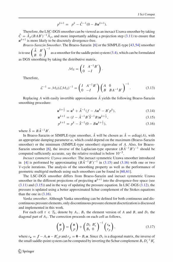
Vanka smoother. Although Vanka smoothing can be defined for both continuous and dis-continuous pressure elements, only discontinuous pressure element discretization is discussedand implemented in this work.

For each cell τ ∈ Th , denote by Aτ , Bτ the element version of A and B, and Dτ thediagonal part of Aτ . The correction proceeds on each cell as follows,

(up

)

=(

up

)

+(

Dτ B ′τBτ 0

)−1 (rurp

)

, (3.17)

where ru = f − Aτ u− B ′τ p and rp = 0− Bτ u. Since Dτ is a diagonal matrix, the inverse ofthe small saddle-point system can be computed by inverting the Schur complement Bτ D−1

τ B ′τ

123

J Sci Comput

which is a matrix of small size. Suitable damping (under-relaxation) can be used to furtherimprove efficiency and ensure the smoothing property; see [58].

Vanka smoother can be viewed as a block-wise Gauss–Seidel procedure of the Braess-Sarazin smoother. Therefore the difference of LSC-DGS smoother with Vanka smoothermainly lies in the different way of updating pressure and enforcing divergence free condition.

4 Auxiliary Space Multigrid Method

In this section we apply the auxiliary space (defect correction) multigrid methods [10,28,29],which consist of an effective smoothing and a simpler discretization serving as a coarse gridcorrection, to the Stokes equations. Since the MAC scheme is only defined on uniform grids,we restrict ourself to the finite element discretization on the rectangular grids in this section.Similar approaches shall work if we have appropriate generalizations of the MAC schemeand corresponding DGS to triangular grids.

4.1 Transfer Operators

We introduce the transfer operators between a finite element fine-space and the MACauxiliary-space. One virtue of ASMG is the simplification of the implementation. The useronly needs to code the geometric multigrid for MAC, a fine grid smoother, and transferoperators from the discretization of consideration to MAC.

In regard to the prolongation (interpolation) operators, many prolongation methods couldbe used. Fortunately, for the auxiliary space multigrid methods, the simplest of these isquite effective. For this reason, we apply bilinear interpolation of neighboring auxiliary-space unknowns in the MAC staggered grid. Figure 2 shows an example of the prolongationfor u from the MAC space to the bi-quadratic Q2 space. The prolongation operator takesMAC auxiliary-space vectors ([· · · , u1, u2, u3, u4, · · · ]t ) and produces Q2 fine-space vec-tors ([· · · , u5, u6, u7, u8, · · · ]t ) according to the following rule:

u5 = u3, u6 = 1

2(u1 + u3), u7 = 1

2(u3 + u4), u8 = 1

4(u1 + u2 + u3 + u4).

The prolongation operator for v can be defined in a similar way. Piecewise constant(first-order) interpolation for the p variables is adopted here because of its simplicity and

(a) (b)

Fig. 2 Sketch of the prolongation from the MAC to Q2. a MAC auxiliary-space points 1, 2, 3, 4. b MACauxiliary-space points 1, 2, 3, 4 and Q2 fine-space points 5, 6, 7, 8, etc

123

J Sci Comput

effectiveness. For the bi-linear Q1 element approximation of the pressure, we use theaverage of the pressure on the four cells sharing a vertex. For the discontinuous pres-sure space Pdc

1 defined linearly in each element, the degree of freedom approximates thecell center value takes the constant pressure from the MAC, while the degree of freedomapproximate the derivatives take values of zero. The interpolation operator will be denotedby IFE

MAC.We choose the restriction operator as the transpose of the prolongation operator divided

by h2 which transfers the residual of the finite element discretizations to that of the finitedifference discretization. The restriction operator will be denoted by RMAC

FE .

4.2 Multigrid Procedure

With the transfer operators defined in the previous subsection, one V-cycle multigrid proce-dure can be summarized in the following algorithm.

Algorithm 4.1. x ← asmg-Vcycle(ν1, ν2, x, b)

1. Relax ν1 steps on LFE y = b with initial guess x.2. Form the FE fine-space residual

r = b− LFE x

and restrict it to the MAC auxiliary-space rMAC = RMACFE r.

3. Solve the MAC auxiliary-space residual equation

LMACeMAC = rMAC

with one multigrid F-cycle procedure.4. Interpolate the MAC auxiliary-space error to the FE fine-space by e =

IFEMACeMAC and correct the FE fine-space approximation by:

x ← x + e.

5. Relax ν2 steps on LFE y = b with initial guess x.

We refer to the multigrid method based on asmg-Vcycle as asmg(ν1,ν2). In the frame-work of defect correction multigrid, the smoothing steps in (1) and (5) can be zero, i.e.,asmg(0, 0) or it could be replaced by the smoothing for LMAC. However, such a schemediverges for all finite elements we have tested. An additional and effective smoothing for thefinite element discretization is really necessary and thus our method is in the sprit of auxiliaryspace method [57]. On solving the MAC auxiliary-space problem, one pre-smoothing andpost-smoothing are used for the F-cycle, i.e., F(1, 1). We can also replace F-cycle withV-cycle or W-cycle. According to our numerical test, F(1, 1) performs equivalently well asV(2, 2) or W(1, 1) cycles in step 3 of asmg-Vcycle.

5 Numerical Experiment

The Stokes system to be solved is

Lx =(

A B ′B 0

) (up

)

=(

f0

)

:= b. (5.1)

123

J Sci Comput

The selected stopping criterion is

‖r i‖l2/‖r0‖l2 < tol,

where tol is a tolerance which will be specified later for each example, and r i = b−Lxi , formultigrid methods and r i = P−1(b− Lxi ), for preconditioned GMRES/MINRES methodwith block or block-triangular preconditioner P introduced in a moment. Zero initial guessis chosen for all tests. The estimates for asymptotic contraction factors (rate) are the averagesof relative residual (‖r3+i‖l2/‖r3‖l2)1/ i over all steps after the third step. The reason startingfrom step 3 rather than step 0 is that asymptotic behavior often appears after a few iterations.

All of our algorithms are implemented using MATLAB. The built-in GMRES/MINRESfunctions are used for the Krylov subspace methods. The finite element matrices on triangulargrids and rectangular grids are assembled using the software iFEM [16] and IFISS [49],respectively. The AMG/MG implemented in the software package iFEM is used for Poissonsolvers. All tests are run on a laptop with 2.50GHz Intel(R) Core(TM) i5-2520M processor.

For all tests, the iteration steps and CPU time of each solver are listed in tables. Thecode has been optimized using vectorization technique so that the CPU time could be agood indicator of the efficiency. To further relieve the affect of programming language andhardware, the operation count is also included. The presentation follows closely the paperby Elman [19].

5.1 Krylov Subspace Methods with Block Preconditioners

For comparison, we will test the Krylov subspace methods with popular block precondition-ers. For the Stokes equations, the classical block-diagonal preconditioner for MINRES [19]method is

P =(

A 00 B A−1 B ′

)

,

and the block-triangular preconditioner [19,26] for GMRES method is

P =(

A B ′0 −B A−1 B ′

)

.

The block preconditioning requires the solution of two systems of equations with matricesA and B A−1 B ′ at each GMRES/MINRES iteration. If P−1 is computed exactly, the precon-ditioned Krylov methods converges in two or three steps [36]. For practical implementations,the Schur complement B A−1 B ′ is replaced by the mass matrix Mp of the pressure space.For discontinuous pressure space, Mp is block diagonal and easy to invert. For continu-ous pressure space, say Q1, the mass matrix Mp can be further replaced by its diagonalmatrix [22].

One geometrical multigrid V-cycle is used to invert the Laplacian operator A of thevelocity. ASMG is also applied in this step. For example, for Q2 element, one Gauss–Seidelsmoothing for Q2 element plus an F-cycle for P1 element serving as the auxiliary spacecorrection.

5.2 Operation Count

Simple comparison of iteration steps and CPU time may not be fair since the performance ofa specific method depends on the implementation and testing environment: the programminglanguage, optimization of codes, and the hardware (memory and cache), etc. To fairly compare

123

J Sci Comput

Table 1 The operations used for each smoother/preconditioner

Smoother/Precond. Matrix-vector product required

LSCDGS 2A 2B 2B′ A−1p A−1

p

DGS (M in (3.6)) A 2B 2B′ A−1p 2D−1

u D−1p

DGS (M in (3.7)) A B 2B′ A−1p An

Vanka N Aτ 3N Bτ N B′τ 2N D−1τ

Inexact Sym. Uzawa A B 2B′ A−1 VB A−1 B′ (1, 1)

Block-diag precond. VA(1, 1) D−1p

Block-tri precond. VA(1, 1) D−1p B′

Table 2 The number of operations for smoothers and preconditioners

Smoother/preconditioner Q⊥1 − P0 P B1 − P1 Q2 − Pdc

1 Q2 − Q1 P iso2 − P1

MAC one F-cycle 2.8L 1.9L 0.4L 0.4L 0.4LLSCDGS 2.3L 2.4L 2.2L 2.2L 2.2LDGS 1.3L 1.6L 1.5L 1.5L 1.5LVanka 2.4L - 2.5L - -

Inexact Sym. Uzawa 1.7L 2.6L 1.7L 1.7L 1.7LBlock-diag precond. 2.9L 1L 2.0L 2.1L 2.1LBlock-tri precond. 3.0L 1.3L 2.2L 2.3L 2.3L

Table 3 Cost for one multigrid cycle or one step of the preconditioned Krylov subspace methods

Methods Q⊥1 − P0 Pb1 − P1 Q2 − Pdc

1 Q2 − Q1 P iso2 − P1

MG-LSCDGS 8.5L 7.7L 5.8L 5.8L 5.8LMG-DGS 6.4L 6.1L 4.4L 4.4L 4.4LMG-Vanka 8.6L - 6.4L - -

MG-iUzawa 7.2L 8.1L 4.8L 4.8L 4.8LMINRES 4.7L 2.8L 3.3L 3.3L 3.3LGMRES 4.0L 2.3L 3.2L 3.3L 3.3L

the efficiency of different solvers, following Elman [19], we list the operation count of eachmethod but only consider the dominating portion of the matrix-vector multiplication. We useone matrix-vector product Lx as a unit, which consists of matrix-vector multiplications ofA, B, and B ′. The cost of a matrix-vector product is estimated to be the number of non-zerosin the matrix used.

We gather the matrix-vector products used in different smoothers and preconditioners inTable 1 and present the costs of smoothers and preconditioners in Table 2. The costs for onemultigrid cycle asmg(1,1) and Krylov subspace iteration are given in Table 3. For multigridmethods, the costs of one V(1, 1)-cycle and F(1, 1)-cycle step are estimated as 11/3 and 9/2work units, respectively, including one residual evaluation on the finest grid; see e.g., [15,50].Since the iteration cost for each step of GMRES is not linear, we only count the cost for the

123

J Sci Comput

Table 4 Example 1. The number of iterations and CPU time (in parentheses) of the asmg multigrid methodwith different smoothers and preconditioned Krylov subspace methods for solving the system (5.1)

Smoother h Q⊥1 − P0 Pb1 − P1 Q2 − Pdc

1 Q2 − Q1 P iso2 − P1

1/64 6 (0.07 s) 10 (0.22 s) 7 (0.25 s) 10 (0.30 s) 13 (0.35 s)

LSC-DGS 1/128 5 (0.23 s) 10 (0.78 s) 7 (0.97 s) 9 (1.00 s) 13 (1.30 s)

1/256 5 (0.90 s) 10 (3.03 s) 7 (4.40 s) 9 (4.01 s) 12 (4.81 s)

1/64 9 (0.13 s) 23 (0.39 s) 11 (0.31 s) 21 (0.84 s) 29 (1.20 s)

DGS 1/128 9 (0.40 s) 23 (1.41 s) 11 (1.15 s) 20 (2.89 s) 28 (4.03 s)

1/256 9 (1.63 s) 22 (5.21 s) 11 (4.51 s) 20 (10.7 s) 27 (12.5 s)

1/64 5 (0.06 s) – 6 (0.24 s) – –

Vanka 1/128 5 (0.24 s) – 6 (0.94 s) – –

1/256 5 (0.89 s) – 6 (4.30 s) – –

1/64 11 (0.24 s) 11 (0.33 s) 9 (0.32 s) 14 (0.56 s) 20 (0.68 s)

iUzawa 1/128 12 (1.67 s) 12 (1.28 s) 9 (1.11 s) 14 (2.76 s) 20 (2.96 s)

1/256 12 (5.66 s) 12 (7.90 s) 9 (4.23 s) 15 (9.31 s) 21 (10.3 s)

Diag-block 1/64 46 (0.55 s) 37 (0.30 s) 30 (0.74 s) 50 (0.85 s) 47 (0.85 s)

precond. 1/128 46 (1.25 s) 37 (1.25 s) 30 (3.01 s) 48 (2.30 s) 45 (2.30 s)

(MINRES) 1/256 44 (5.07 s) 37 (4.90 s) 32 (11.7 s) 48 (10.2 s) 43 (10.2 s)

Tri-block 1/64 25 (0.60 s) 24 (1.14 s) 22 (0.96 s) 32 (1.45 s) 24 (1.05 s)

precond. 1/128 26 (1.64 s) 25 (4.99 s) 22 (4.32 s) 32 (5.35 s) 19 (4.35 s)

(GMRES) 1/256 27 (6.64 s) 25 (20.3 s) 23 (14.7 s) 33 (22.8 s) 18 (17.8 s)

preconditioner and the multiplication of L in Table 3 for GMRES. Additional cost will becounted for the whole iteration process in the numerical experiment.

The counting is based on an N × N uniform rectangular grid. For general unstructuredgrids, the number of operation for each method depends also on the topology of the underlinegrids and could be slightly different.

5.3 Numerical Examples: Rectangular Grids

The first numerical experiment is carried out to show the efficiency of the LSC-DGS smootherand the ASMG method. The grids considered are the uniform rectangular grids. A uniformtriangulation can be obtained by drawing the diagonal with positive slope in each rectangularcell. Five stable finite element discretizations on uniform rectangular or triangular grids areconsidered: Q⊥1 −P0, Pb

1 −P1, Q2−Q1, P iso2 −P1 and Q2−Pdc

1 . Here, Q⊥1 denotes rotatednonconforming bilinear element [46], Pb

1 stands for the piecewise linear and continuousspace with cubic element bubbles [1] on a uniform triangulation, P iso

2 is the linear elementon a uniform refined triangulation, and Pdc

1 represents disconutinous element in each smallrectangle [22]. Other low order elements including Q2−Q0, Qiso

2 −Q0, etc., have also beentested and similar conclusions were drawn. Since the rate of convergence of these schemesare lower than the MAC scheme, results for these schemes are not reported here.

For the ASMG algorithm, the solver for the MAC scheme is one F(1, 1) cycle, i.e., anF-cycle with one V(1, 1) in each level. Only asmg(1, 1) is tested. The basic set up for thesmoothers is listed below.

123

J Sci Comput

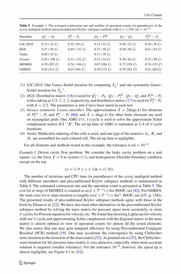
Table 5 Example 1. The averaged contraction rate and number of operation counts (in parentheses) of theasmg multigrid method and preconditioned Krylov subspace methods with h = 1/256, tol = 10−6

Smoother Q⊥1 − P0 Pb1 − P1 Q2 − Pdc

1 Q2 − Q1 P iso2 − P1

LSC-DGS 0.12 ( 43 L) 0.33 ( 85 L) 0.13 ( 41 L) 0.28 ( 52 L) 0.30 ( 56 L)

DGS 0.27 ( 58 L) 0.49 ( 132 L) 0.37 ( 48 L) 0.58 ( 88 L) 0.61 ( 93 L)

Vanka 0.05 ( 43 L) – 0.11 ( 38 L) – –

iUzawa 0.29 ( 108 L) 0.31 ( 122 L) 0.21 ( 54 L) 0.30 ( 84 L) 0.35 ( 98 L)

MINRES 0.70 (207 L) 0.74 ( 104 L) 0.67 (106 L) 0.77 (158 L) 0.74 (152 L)

GMRES 0.42 (513 L) 0.63 (382 L) 0.39 (172 L) 0.70 (281 L) 0.51 (201L)

(1) LSC-DGS: One Gauss–Seidel iteration for computing A−1p and one symmetric Gauss–

Seidel iteration for A−1p .

(2) DGS: Distributive matrix (3.6) is used for Q⊥1 − P0, Q2− Pdc1 , Q2−Q1 and P iso

2 − P1

with α taking as 3/2, 1, 2, 2, respectively, and distributive matrix (3.7) is used for Pb1 −P1

with β = 3/2. The parameters α and β have been tuned in each test.(3) Inexact symmetric Uzawa smoother: The approximation A = 2diag(A) for elements

of P iso2 − P1 and Pb

1 − P1 [60], and A = diag(A) for other finite elements are usedon rectangular grids. One AMG V(1, 1)-cycle is used to solve the approximate Schurcomplement matrix B A−1 B ′. The set up time of AMG is estimated as 1/4 of V-cycleiterations.

(4) Vanka: Multicolor ordering of the cells is used, and one type of the matrices Aτ , Bτ andDτ are assembled for each colored cell. The set up time is negligible.

For all elements and methods tested in this example, the tolerance is tol = 10−6.

Example 1 Driven cavity flow problem. We consider the leaky cavity problem on a unitsquare, i.e, the force f = 0 in system (1.1), and homogenous Dirichlet boundary conditionexcept on the top

{y = 1; 0 ≤ x ≤ 1|u = (1, 0)}.The number of iterations and CPU time (in parentheses) of the asmg multigrid method

with different smoothers and preconditioned Krylov subspace methods is summarized inTable 4. The estimated contraction rate and the operation count is presented in Table 5. Thecost for m steps of MINRES is counted as m(L+P−1)+ 6m·#DOF; see [42]. For GMRES,the total costs for m steps iteration is roughly m(L+P−1)+ 4m2· #DOF; see ([47, p. 158]).The presented results of preconditioned Krylov subspace methods agree with those in thebook by Elman et al. [22]. We have also tried other alternatives in the preconditioned Krylovsubspace method by solving the mass matrix for pressure space more accurately, or moreV-cycles for Poisson equation for velocity, etc. We found that inverting Laplacian for velocitywith one V-cycle and approximating Schur complement with the diagonal matrix of the massmatrix is almost optimal in view of operation counts for almost all the tested elements.We also notice that one may gain marginal efficiency by using Preconditioned ConjugateResidual (PCR) method [19]. One may accelerate the convergence by using Chebyshevsemi-iteration in the inversion of the mass matrix [52]. As pointed out in [52], the Chebychev-semi-iteration for the pressure mass matrix is very attractive, especially when more accuratesolution is required (smaller tolerance). For the tolerance 10−6, however, the speed up isalmost negligible, see Figure 4.1 in [52].

123

J Sci Comput

0 20 40 60 80 100 120 140 160

10−6

10−5

10−4

10−3

10−2

10−1

100

10−6

10−5

10−4

10−3

10−2

10−1

100

rela

tive

resi

dual

work unit (L)

Q2−P

−1: comparison of operation cost for various methods

MG/LSCDGSMG/DGSMG/VankaMG/iUzawaMINRESGMRES

0 50 100 150 200 250

rela

tive

resi

dual

work unit (L)

Q2−Q

1: comparison of operation cost for various methods

MG/LSCDGSMG/DGSMG/iUzawaMINRESGMRES

Fig. 3 Comparison of operation counts for multigrid method and Krylov subspace method. a Q2 − Pdc1 .

b Q2 − Q1 (Example 1)

The residual norms against operation counts of different solvers for Q2−Pdc1 and Q2−Q1

is plotted in Fig. 3. Similar behavior is also observed for other elements and thus only twotypical finite element pairs, one with continuous and another with discontinuous pressurespace, are shown here.

We have tested other settings having analytical solutions, similar behavior was observed.We shall not report them.

Based on these results, we may draw the following conclusion for the performance onuniform grids.

(1) All methods are uniformly convergent with respect to h. Namely all of them are ofoptimal linear complexity.

(2) Multigrid asmg(1,1), i.e., combination of smoothing in the FE space and correctionusing multigrid for MAC scheme, outperforms the popular preconditioned Krylov spacesmethods. For example, ASMG using LSC-DGS is in average two or three times fasterthan preconditioned MINRES.

(3) Among the various smoothers, LSC-DGS smoother is the most efficient one in mostcases. For discontinuous pressure, Vanka smoothing is the best in terms of operationcounts, which in part is due to the multicolor ordering for the grids. For continuouspressure spaces, due to the continuity of the pressure, it is not easy to code Vankasmoothing for overlapping patches [33,34]. In general, geometric and basis informationis needed to code an effective Vanka smoother while LSC-DGS only uses the givenmatrices and thus is more user-friendly.

5.4 Numerical Examples: Triangular Grids

For general triangular grids, we do not have efficient MG-DGS methods for MAC-typeschemes. Therefore we test the standard V-cycle or W-cycle multigrid based on the LSC-DGS smoother. For saddle point problems, we expect the uniform convergence of W-cyclewith enough smoothing steps while V-cycle is less stable. In [60] Zulehner pointed out thatthe contraction rates of multigrid methods (using an inexact Uzawa smoother) are certainlystill unsatisfactory for unstructured grids. Therefore we apply tests on three different kindsof grids including both structured and unstructured grids.

123

J Sci Comput

(a) (b) (c)

Fig. 4 Three types of meshes used in Example 2

As in [6,60], we consider the P iso2 − P1 element (modified Taylor-Hood element) dis-

cretization: linear shape-functions on a triangular grid for the pressure and linear shape-functions for the velocity on an uniformly refined mesh (where each triangle is divided intofour similar small triangles) [14,45]. The performance of other elements are similar. Thesymbol “×” in the following tables means that the corresponding algorithm diverges.

Example 2 Classical multigrid methods with LSC-DGS smoother on triangular grids. Thisexample is taken from [6,60]. The analytical solution u and p are chosen as follows:

u(x, y) =(

sin x sin ycos x cos y

)

, p(x, y) = 2 cos x sin y + C,

where C is chosen for each specific example such that p ∈ L20(�).

Three different types of meshes are considered and the coarsest meshes are plotted inFig 4. The level k in Tables 6, 7, 8 stands for k times uniform refinement of the coarsestmesh. For the circular domain, after each refinement, the boundary nodes are projected ontothe circle and thus results in non-nested finite element spaces. The grid in Fig. 4(b) is takenfrom [6,60].

The choice of tolerance is tol = 10−8 in this example.

Example 2.1 Structured grids of a square domain. The performance of both V-cycles andW-cycles is present in Table 6 for the structured grid shown in Fig. 4 (a). In the LSC-DGS smoother, A−1 is chosen as one Gauss–Seidel iteration, and A−1

p is one symmetricGauss–Seidel iteration. In the inexact symmetric Uzawa smoother, following Zulehner [60],the smoother A is chosen as A = 2diag(A), and one V(2, 2)-cycle is used to solve theapproximate Schur complement S = B A−1 B ′. For comparison, the numerical result forASMG-LSC-DGS is also included in Table 6.

Example 2.2 Unstructured grids of a square domain. The numerical results are reported inTable 7 for the unstructured grids shown in Fig. 4(b). In the LSC-DGS smoother, A−1 is oneGauss–Seidel iteration, while A−1

p is chosen as one V(2, 2)-cycle, since more accurate solveris required to guarantee the commutator W is small for the unstructured grids. In the inexactsymmetric Uzawa smoother, A is chosen as A = 2diag(A), and two V(2, 2)-cycles are usedto solve the approximate Schur complement S = B A−1 B ′ to ensure the Schur complementB A−1 B ′ being solved accurately enough.

For this example, only W-cycle is reported since V-cycle converge but not uniformlywithin 5 steps of pre-smoothing and post-smoothing for both of MG-LSCDGS and

123

J Sci Comput

Table 6 Example 2.1: structured grids of a square domain

level #DOF V-cycle W-cycle

(1,1) (2,2) (1,1) (2,2)

(a) MG-LSC-DGS

5 37,507 21 (0.68s) 10 (0.44s) 10 (0.51s) 7 (0.56s)

6 148,739 31 (3.64s) 10 (1.66s) 10 (2.07s) 7 (2.32s)

7 592,387 58 (27.1s) 10 (7.07s) 10 (7.22s) 7 (9.66s)

(b) ASMG-LSC-DGS

5 37,507 16 (0.43s) 13 (0.51s)

6 148,739 16 (1.42s) 13 (1.72s)

7 592,387 16 (5.80s) 13 (6.18s)

(c) MG-iUzawa

5 37,507 × 16 (1.21s) 29 (3.12s) 14 (2.30s)

6 148,739 × 16 (3.58s) 29 (8.21s) 14 (6.73s)

7 592,387 × 16 (12.9s) 29 (27.1s) 14 (22.6s)

Comparison of the iterations for three different kinds of multigrid solvers: (a) MG-LSC-DGS, (b) ASMG-LSC-DGS, and (c) MG-iUzawa (tol = 10−8)

Table 7 Example 2.2: Unstructured grids of a square domain

level #DOF W-cycle

(1,1) (2,2) (3,3) (4,4)

(a) MG-LSC-DGS

5 41,875 35 (4.13s) 18 (3.28s) 13 (3.61s) 11 (4.04s)

6 166,691 34 (16.2s) 18 (15.3s) 13 (15.9s) 11 (16.1s)

7 665,155 34 (65.5s) 18 (56.7s) 13 (58.8s) 11 (63.6s)

(b) MG-iUzawa

5 41,875 × × 33 (11.2s) 26 (10.9s)

6 166,691 × × 33 (38.3s) 25 (37.1s)

7 665,155 × × 33 (126s) 25 (120s)

Comparison of the iterations for two different kinds of multigrid solvers: (a) MG-LSC-DGS and (b) MG-iUzawa (tol = 10−8)

MG-iUzawa. Due to the poor mesh quality, both the cost of one iteration and the number ofiterations increases comparing to the structured grids case.

We estimate the operation cost for LSC-DGS smoother and inexact symmetric Uzawasmoother in the unstructured grid case for P iso

2 − P1 element. The cost of one V(2, 2)-cycle and W(3, 3)-cycle for inverting a sparse matrix with N non-zeros is about 19/3N and13N , respectively [50]. The cost for one LSC-DGS smoother is about 2.4L, and the cost forone inexact symmetric Uzawa smoother is about 2.6L. Therefore, the cost of one multigridW(3, 3)-cycle is 31.2L and 33.8L for MG-LSC-DGS and MG-iUzawa, respectively. Thecomparison is plotted in Fig. 5 and the result for MG-iUzawa is consistent with that in [60].

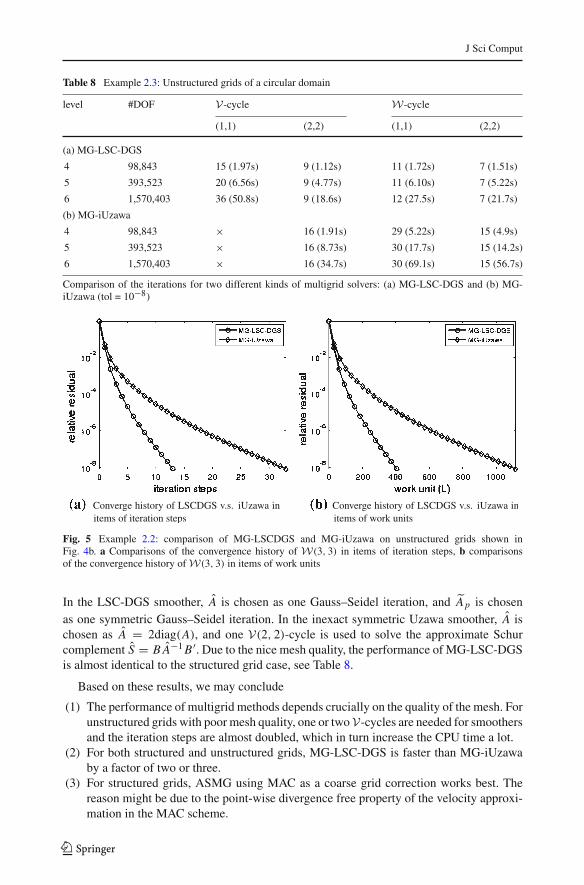
Example 2.3 Unstructured grids of a circular domain. This example is devoted to show theperformance of multigrid V-cycle and W-cycle for a unstructured grid of a circular domain.

123

J Sci Comput

Table 8 Example 2.3: Unstructured grids of a circular domain

level #DOF V-cycle W-cycle

(1,1) (2,2) (1,1) (2,2)

(a) MG-LSC-DGS

4 98,843 15 (1.97s) 9 (1.12s) 11 (1.72s) 7 (1.51s)

5 393,523 20 (6.56s) 9 (4.77s) 11 (6.10s) 7 (5.22s)

6 1,570,403 36 (50.8s) 9 (18.6s) 12 (27.5s) 7 (21.7s)

(b) MG-iUzawa

4 98,843 × 16 (1.91s) 29 (5.22s) 15 (4.9s)

5 393,523 × 16 (8.73s) 30 (17.7s) 15 (14.2s)

6 1,570,403 × 16 (34.7s) 30 (69.1s) 15 (56.7s)

Comparison of the iterations for two different kinds of multigrid solvers: (a) MG-LSC-DGS and (b) MG-iUzawa (tol = 10−8)

Fig. 5 Example 2.2: comparison of MG-LSCDGS and MG-iUzawa on unstructured grids shown inFig. 4b. a Comparisons of the convergence history of W(3, 3) in items of iteration steps, b comparisonsof the convergence history of W(3, 3) in items of work units

In the LSC-DGS smoother, A is chosen as one Gauss–Seidel iteration, and A p is chosenas one symmetric Gauss–Seidel iteration. In the inexact symmetric Uzawa smoother, A ischosen as A = 2diag(A), and one V(2, 2)-cycle is used to solve the approximate Schurcomplement S = B A−1 B ′. Due to the nice mesh quality, the performance of MG-LSC-DGSis almost identical to the structured grid case, see Table 8.

Based on these results, we may conclude

(1) The performance of multigrid methods depends crucially on the quality of the mesh. Forunstructured grids with poor mesh quality, one or two V-cycles are needed for smoothersand the iteration steps are almost doubled, which in turn increase the CPU time a lot.

(2) For both structured and unstructured grids, MG-LSC-DGS is faster than MG-iUzawaby a factor of two or three.

(3) For structured grids, ASMG using MAC as a coarse grid correction works best. Thereason might be due to the point-wise divergence free property of the velocity approxi-mation in the MAC scheme.

123

J Sci Comput

6 Conclusions and Future Research

The Stokes system is the first step for the numerical computation of incompressible flowequations. Our method can be extended to the Navier-Stokes equations, since no explicitconstruction of Ap is required. On rectangular grids we will design fast solvers for the MACdiscretization of Navier-Stokes equation with the LSCDGS smoother, combining the ideain [12,13] for the high-Reynolds incompressible flow, and use it as a coarse grid solverto design an efficient multigrid solver for finite element discretization of Navier-Stokesequations.

Another direction is to develop an efficient ASMG for triangular grids. We will firstinvestigate the generalization of MAC to triangular grids [23,38] and design correspondingDGS-type smoother and multigrid methods.

Acknowledgments The work of the first author was supported by 2010-2012 China Scholarship Coun-cil (CSC). The second author was supported by NSF Grant DMS-1115961, and in part by Department ofEnergy prime award # DE-SC0006903. The authors are grateful to the discussions with Professors A. Brandt,J. Hu, J. Xu, I. Yavneh, and L. Zikatanov. The second author was introduced to DGS by Prof. Yavenh duringthe IMA workshop ‘Numerical Solutions of Partial Differential Equations: Fast Solution Techniques’, Dec2010, and then had further discussion with these experts in the workshop ‘Algebraic Multigrid Methods withApplications to Fluids and Structure Interactions and Other Multi-Physical Systems’ in Kunming Aug 2011.We would also like to thank IMA and Kunming University of Science and Technology for their support andhospitality, as well as for their exciting research atmosphere. The authors also would like to thank two refereesfor their thorough review. The quality of the paper is improved by addressing their constructive comments andsuggestions.

References

1. Arnold, D., Brezzi, F., Fortin, M.: A stable finite element for the Stokes equations. Calcolo 21(4), 337–344(1984)

2. Auzinger, W., Stetter, H.: Defect correction and multigrid iterations. In: Hackbusch, W., Trottenberg, U.(eds.) Multigrid Methods, vol. 960, pp. 327–351 (1982)

3. Bacuta, C., Vassilevski, P., Zhang, S.: A new approach for solving Stokes systems arising from a distrib-utive relaxation method. Numer. Methods Partial Differ. Equ. 27(4), 898–914 (2011)

4. Bank, R., Welfert, B., Yserentant, H.: A class of iterative methods for solving saddle point problems.Numerische Mathematik 56(7), 645–666 (1989)

5. Benzi, M., Golub, G., Liesen, J.: Numerical solution of saddle point problems. Acta Numerica. 14(1),1–137 (2005)

6. Braess, D., Sarazin, R.: An efficient smoother for the Stokes problem. Appl. Numer. Math. 23(1), 3–19(1997)

7. Bramble, J., Pasciak, J.: A preconditioning technique for indefinite systems resulting from mixed approx-imations of elliptic problems. Math. Comput. 50(181), 1–17 (1988)

8. Bramble, J., Pasciak, J.: Iterative techniques for time dependent Stokes problems. Comput. Math. Appl.33(1–2), 13–30 (1997)

9. Brandt, A.: Multi-level adaptive solutions to boundary-value problems. Math. Comp. 31, 333–390 (1977)10. Brandt, A.: Multigrid techniques: 1984 guide with applications to fluid dynamics. Ges. für Mathematik

u, Datenverarbeitung (1984)11. Brandt, A., Dinar, N.: Multi-grid Solutions to Elliptic Llow Problems. Institute for Computer Applications

in Science and Engineering, NASA Langley Research Center (1979)12. Brandt, A., Yavneh, I.: On multigrid solution of high-Reynolds incompressible entering flows. J. Comput.

Phys. 101, 151–164 (1992)13. Brandt, A., Yavneh, I.: Accelerating multigrid convergence and high-Reynolds recirculating flows. SIAM

J. Sci. Comput. 14, 607–626 (1993)14. Brezzi, F., Fortin, M.: Mixed and Hybrid Finite Element Methods. Springer, Berlin (1991)15. Briggs, W., McCormick, S., et al.: A Multigrid Tutorial, vol. 72. Society for Industrial Mathematics (2000)

123

J Sci Comput

16. Chen, L.: iFEM: An Integrated Finite Element Methods Package in MATLAB. University of Californiaat Irvine, Technical Report (2009)

17. Chen, L.: Finite difference method (MAC) for Stokes equations. Lecture notes (2012)18. Chen, L., Wang, M., Zhong, L.: Second order accuracy of a MAC scheme for the Stokes equations (in

preparation) (2013)19. Elman, H.: Multigrid and Krylov subspace methods for the discrete Stokes equations. Int. J. Numer.

Methods Fluids 22(8), 755–770 (1996)20. Elman, H.: Preconditioning for the steady-state Navier-Stokes equations with low viscosity. SIAM J. Sci.

Comput. 20(4), 1299–1316 (1999)21. Elman, H., Howle, V., Shadid, J., Shuttleworth, R., Tuminaro, R.: Block preconditioners based on approx-

imate commutators. SIAM J. Sci. Comput. 27(5), 1651–1668 (2006)22. Elman, H., Silvester, D., Wathen, A.: Finite Elements and Fast Iterative Solvers: With Applications in

Incompressible Fluid Dynamics. Oxford University Press, USA (2005)23. Eymard, R., Fuhrmann, J., Linke, A.: MAC schemes on triangular meshes. Finite Vol Complex Appl VI

Problems Perspect. 4, 399–407 (2011)24. Gaspar, F., Lisbona, F., Oosterlee, C., Vabishchevich, P.: An efficient multigrid solver for a reformulated

version of the poroelasticity system. Comput. Methods Appl. Mech. Eng. 196(8), 1447–1457 (2007)25. Gaspar, F., Lisbona, F., Oosterlee, C., Wienands, R.: A systematic comparison of coupled and distributive

smoothing in multigrid for the poroelasticity system. Numer. Linear Algebra Appl. 11(2–3), 93–113(2004)

26. Geenen, T., Vuik, C., Segal, G., MacLachlan, S.: On iterative methods for the incompressible Stokesproblem. Int. J. Numer. Methods fluids 65(10), 1180–1200 (2011)

27. Gresho, P., Sani, R.: On pressure boundary conditions for the incompressible Navier-Stokes equations.Int. J. Numer. Methods Fluids 7(10), 1111–1145 (1987)

28. Hackbusch, W.: On multigrid iterations with defect correction. In: Hackbusch, W., Trottenberg, U., (eds.)Multigrid Methods, pp. 461–473 (1982)

29. Hackbusch, W.: Multi-grid Methods and Applications, vol. 4 of Springer Series in Computational Math-ematics (1985)

30. Han, H., Wu, X.: A new mixed finite element formulation and the MAC method for the Stokes equations.SIAM J. Numer. Anal. 35(2), 560–571 (1998)

31. Harlow, F., Welch, J., et al.: Numerical calculation of time-dependent viscous incompressible flow offluid with free surface. Phys. fluids 8(12), 2182 (1965)

32. Hu, Q., Zou, J.: Two new variants of nonlinear inexact Uzawa algorithms for saddle-point problems.Numer. Math. 93(2), 333–359 (2002)

33. John, V., Matthies, G.: Higher-order finite element discretizations in a benchmark problem for incom-pressible flows. Int. J. Numer. Methods Fluids 37(8), 885–903 (2001)

34. Larin, M., Reusken, A.: A comparative study of efficient iterative solvers for generalized stokes equations.Numer. Linear Algebra Appl. 15(1), 13–34 (2008)

35. Maitre, J.F., Musy, F., Nigòn, P.: Fast solver for the Stokes equations using multigrid with a Uzawasmoother. Notes Numer. Fluid Mech. 11, 77–83 (1985)

36. Murphy, M., Golub, G., Wathen, A.: A note on preconditioning for indefinite linear systems. SIAM J.Sci. Comput. 21(6), 1969–1972 (1999)

37. Nicolaides, R.: Analysis and convergence of the MAC scheme I. The linear problem. SIAM J. Numer.Anal. 29(6), 1579–1591 (1992)

38. Nicolaides, R., Porsching, T., Hall, C.: Covolume Methods in Computational Fluid Dynamics, vol. 279.Wiley, New York (1995)

39. Nicolaides, R., Wu, X.: Analysis and convergence of the MAC scheme II. Navier-Stokes equations. Math.Comput. 65(213), 29–44 (1996)

40. Niestegge, A., Witsch, K.: Analysis of a multigrid Stokes solver. Appl. Math. Comput. 35(3), 291–303(1990)

41. Oosterlee, C., Lorenz, F.: Multigrid methods for the Stokes system. Comput. Sci. Eng. 8(6), 34–43 (2006)42. Paige, C., Saunders, M.: Solution of sparse indefinite systems of linear equations. SIAM J. Numer. Anal.

12(4), 617–629 (1975)43. Patankar, S., Spalding, D.: A calculation procedure for heat, mass and momentum transfer in three-

dimensional parabolic flows. Int. J. Heat Mass Transf. 15(10), 1787–1806 (1972)44. Peric, M., Kessler, R., Scheuerer, G.: Comparison of finite-volume numerical methods with staggered

and colocated grids. Comput. Fluids 16(4), 389–403 (1988)45. Pironneau, O.: Finite Element Methods for Fluids. NASA STI/Recon technical report A, vol. 90, p. 24264

(1989)

123

J Sci Comput

46. Rannacher, R., Turek, S.: Simple nonconforming quadrilateral Stokes element. Numer. Methods PartialDiffer. Equ. 8(2), 97–111 (1992)

47. Saad, Y.: Iterative Methods for Sparse Linear Systems. PWS Pub Co, USA (1996)48. Shaw, G., Sivaloganathan, S.: On the smoothing properties of the simple pressure-correction algorithm.

Int. J. Numer. Methods Fluids 8(4), 441–461 (1988)49. Silvester, D., Elman, H., Ramage, A.: Incompressible flow and iterative solver software (IFISS) version

3.1. Available online at http://www.manchester.ac.uk/ifiss (2011)50. Trottenberg, U., Oosterlee, C., Schüller, A.: Multigrid. Academic Press, London (2001)51. Vanka, S.: Block-implicit multigrid solution of Navier-Stokes equations in primitive variables. J. Comput.

Phys. 65(1), 138–158 (1986)52. Wathen, A., Rees, T.: Chebyshev semi-iteration in preconditioning for problems including the mass

matrix. Electron. Trans. Numer. Anal. 34, 125–135 (2009)53. Wienands, R., Gaspar, F., Lisbona, F., Oosterlee, C.: An efficient multigrid solver based on distributive

smoothing for poroelasticity equations. Computing 73(2), 99–119 (2004)54. Wittum, G.: Multi-grid methods for Stokes and Navier-Stokes equations. Numerische Mathematik 54(5),

543–563 (1989)55. Wittum, G.: On the convergence of multi-grid methods with transforming smoothers. Numerische Math-

ematik 57(1), 15–38 (1990)56. Xu, J.: Iterative methods by space decomposition and subspace correction. SIAM Rev. 34(4), 581–613

(1992)57. Xu, J.: The auxiliary space method and optimal multigrid preconditioning techniques for unstructured

grids. Computing 56(3), 215–235 (1996)58. Zhang, L.: A second-order upwinding finite difference scheme for the steady Navier-Stokes equations in

primitive variables in a driven cavity with a multigrid solver. M2AN 24, 133–150 (1990)59. Zhu, Y., Sifakis, E., Teran, J., Brandt, A.: An efficient multigrid method for the simulation of high-

resolution elastic solids. ACM Trans. Graph. (TOG) 29(2), 16 (2010)60. Zulehner, W.: A class of smoothers for saddle point problems. Computing 65(3), 227–246 (2000)61. Zulehner, W.: Analysis of iterative methods for saddle point problems: a unified approach. Math. Comput.

71(238), 479–506 (2002)

123