. • Journal of Hydrology

Journal of Hydrology 187 (1996) 29--43 ELSEVIER

Multifractal analysis of daily spatial rainfall distributions

Jonas Olsson*, Janusz Niemczynowicz

Department of Water Resources Engineering, Institute of Science and Technology, Lurid University, Box 118, S-221 O0 Lund, Sweden

Received 23 December 1993; accepted 19 October 1995

Abstract

The multifractal behavior of daily spatial rainfall distributions observed by a dense gage network in southern Sweden was analyzed by studying the variation of average statistical moments with scale. The data were analyzed both separated into groups depending on the rainfall generating mechanism (warm fronts, cold fronts, and convection, respectively) and pooled into one group representing the total rainfall process in the area. The results indicated that the daily spatial rainfall distributions were well characterized by a multifractal behavior both separated into mechanism groups and pooled into one group. The multifzactal properties, however, displayed distinct differences which were related to physical differences of the rainfall generating mechanisms. The multifractal properties of the total rainfall process agreed well with the properties of the cold front group. Investigations of interpolated grids showed that these well preserve the multifractal behavior of the original data, but modify the multibactal properties.

1. Introduction

The possibility to characterize rainfall by scale invariant (scaling) and fractal properties has been widely investigated during recent years. The early theory of monofractals or simple scaling (e.g. Lovejoy, 1982; Lovejoy and Mandelbrot, 1985), has undergone sub- stantial refinement into the more general and more practicable theory of multif~actals or multiscaling (e.g. Schertzer and Lovejoy, 1987; Gupta and Waymire, 1990; Lovejoy and Schertzer, 1990). It has been shown that multifractal fields may be produced by so-called multiplicative cascade processes where some large scale flux is concentrated into succes- sively smaller spatial units (e.g. Schertzer and I~vejoy, 1987; Gupta and Waymire, 1993). It has been argued that this behavior is expected for the flux of water in the atmosphere

* Corresponding author.

0022-1694,~/$15.00 O 1996 - Elsevier Science B.V. All rights reserved PII S0022-1694(96)03085-5

30 J. Olsso~ J. Niemczynowicz/Journai of Hydrology 187 (1996) 29--43

under the assumption that the Navier-Stokes equations for hydrodynamic turbulence are approximately valid for the atmosphere (e.g. Tessier et al., 1993). There are also empirical observations in favor of a cascade behavior in the atmosphere. The often observed hierarchical structure of rainfall fields, Where large-scale synoptic areas with a low rainfall intensity contain smaller meso-scale areas of higher intensity which in turn contain individual convective cells of even higher intensity, is directly indicative of a cascade type of behavior (e.g. Gupta and Waymire, 1993).

The scaling, generally multifractal, structure of fields produced by a cascade process can be expressed by some statistical relationships (e.g. Gupta and Waymire, 1990; Lovejoy and Schertzer, 1990) which may be very useful in practical rainfall applications. For example, because of the scale independence, the possibility exists to derive statistical information about the rainfall process at scales smaller than the resolution scale of the available data (e.g. Olsson, 1995b). This constitutes an exciting way to deal with the increasing problem of inadequate rainfall data input in hydrological models.

However, before developing practically applicable methods for data processing, the multifractal behavior must be carefully validated on real rainfall data and the number of such investigations is still rather low. Recent investigations have mostly dealt with either radar data (e.g. Gupta and Waymire, 1990, 1993; Lovejoy and Schertzer, 1990, 1991; Tessier et al., 1993; Over and Gupta, 1994), or rainfall time series (e.g. Ladoy et al., 1991, 1993; Olsson et al., 1992, 1993; Rajagopalan and Tarboton, 1993; Hubert et al., 1993; Olsson, 1995a,b).

In most of these studies the rainfall process has been investigated without any attempts to distinguish between observations related to different rainfall generating mechanisms. This is basically due to an inherent conflict between on one hand the overall scale- independence of the multifractal approach and on the other hand the 'classical' meteor- ological approach where certain processes are related to certain scales. Investigations of rainfall time series have, however, indicated that a compromise may be possible: scale- independence within limits related to rainfall properties descending from meteorological and climatological characteristics (e.g. Fraedrich and Larnder, 1993; Oisson et al., 1993). If these characteristics put limits to the scale-independent range it is reasonable to assume that they also influence the multifractal properties within the limits. A possible implication of this is that the multifractal properties of the rainfall process may be different for different geographical regions depending on the dominant rainfall generating mechanism.

In light of the above we choose to use two approaches in the present multifractal investigation. Firstly, spatial rainfall distributions associated with different rainfall gen- erating mechanisms are analyzed separately. Secondly, the 'average' multifractal behavior is investigated by pooling all distributions into one group representing the total rainfall process.

2. Rainfall data

As previously mentioned, most multifractal analyses of spatial rainfall have been per- formed on radar data and very few on rain-gage data. Although radar data are available

J. Oisson, Z N~mczynowiczlJournal of Hydrology 187 (1996) 29--43 31

with a very high spatial resolution, using rain gages still constitute the most reliable way of determining the mounts of rainfall that actually reach the ground surface.

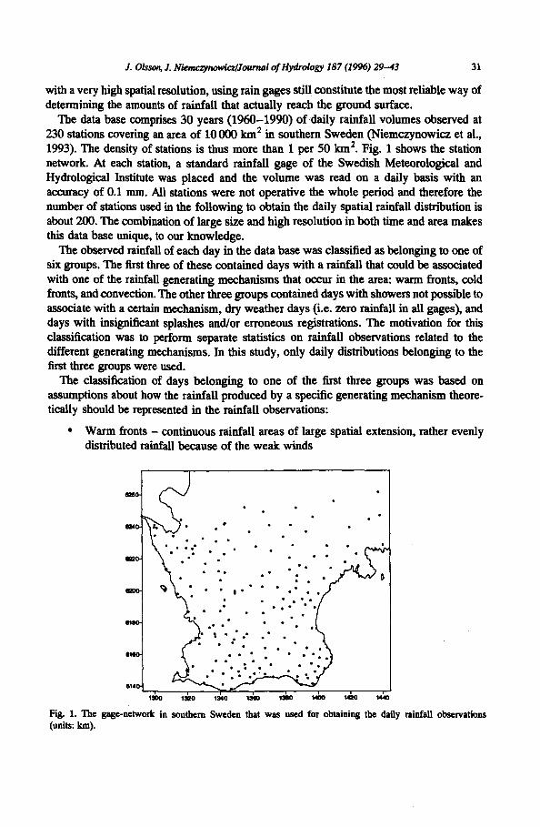
The data base comprises 30 years (1960-1990) of daily rainfall volumes observed at 230 stations covering an area of 10 000 km 2 in southern Sweden (Niemczynowit~ et al., 1993). The density of stations is thus more than I per 50 km 2. Fig. 1 shows the station network. At each station, a standard rainfall gage of the Swedish Meteorological and Hydrological Institute was placed and the volume was read on a daily basis with an accuracy of 0.I mm. All stations were not operative the whole period and therefore the number of stations used in the following to obtain the daily spatial rainfall distribution is about 200. The combination of large size and high resolution in both time and area makes this data base unique, to our knowledge.

The observed rainfall of each day in the data base was classified as belonging to one of six groups. The first three of these contained days with a rainfall that could be associated with one of the rainfall generating mechanisms that occur in the area: warm fronts, cold fronts, and convection. The other three groups contained days with showers not possible to associate with a certain mechanism, dry weather days (i.e. zero rainfall in all gages), and days with insignificant splashes and/or erroneous registrations. The motivation for this classification was to perform separate statistics on rainfall observations related to the different generating mechanisms. In this study, only daily distributions belonging to the first three groups were used.

The classification of days belonging to one of the first three groups was based on assumptions about how the rainfall produced by a specific generating mechanism theore- tically should be represented in the rainfall observations:

• Warm fronts - continuous rainfall areas of large spatial extension, rather evenly distributed rainfall because of the weak winds

i i , ,

~aoo 1 ' , ,o .ts4o .~3eo 1 s o ~ t4~o .,44o

Fig. i. The gage-network in southern Sweden that was used for obtaining the daily rainfall observations (units: km).

32 J. Oisson, J. Niemczynowicz/Journal of Hydrology 187 (1996) 29-43

• Cold fronts - continuous rainfall areas of large spatial extension, larger variability because of the stronger and more turbulent winds

• Convection - smaller, more or less separate rainfall areas displaying a consider- able variability

By studying how clearly these properties were manifested in the daily data it was concluded that the network was well suited to reveal the differences between rainfall observations related to different generating mechanisms. Firstly, the size of the network was such that frontal rainfall generally covers the whole network whereas the rainfall areas generated by convection generally are captured within the network. Secondly, the network density showed to be sufficient to generally capture the differences in rainfall variability for the mechanisms. Thus an automatic classification method, based on the above proper- ties, primarily represented through the share of stations with non-zero registrations and the coefficient of variation of these registrations, was developed (Linderson et al., 1993).

For this study, 6 days belonging to each of the three rainfall generating mechanism groups were selected (18 days in total). It must be emphasized that the rainfall observed on one day may very well have been produced by different mechanisms that have occurred at different times during the day or even simultaneously. Thus, at the above selection, emphasis was put on finding days exhibiting a rainfall distribution that was typical for their respective group. For each of the selected days the meteorological situation was carefully verified by studying synoptic weather maps and written weather descriptions. Table I shows the coefficient of variation and share of stations with non-zero registrations, respectively, for the mechanism groups.

As previously mentioned, the rainfall distributions were both analyzed separated into the above described mechanism groups and pooled into one group representing the total rainfall process. This requires the assumption that the different rainfall generating mechanisms are approximately equally commonly occurring in the region. From the result of the above described classification method, this assumption showed to be fairly well fulfilled.

In practical rainfall applications, however, it is often more convenient to work with regular grids than irregular data. Therefore, apart from studying the data in their irregu- larly spaced form, an investigation of the scaling properties of grids interpolated from the data was conducted. This interpolation will smooth the rainfall distributions and the maximum and minimum value will decrease and increase, respectively, changes that are likely to affect also the scaling properties. Thus it is of interest to study to which extent the scaling properties of the original data are preserved in the interpolated grids.

Table 1 Coefficient of variation (CV) and share of stations with non-zero registrations (SSR) for the daily spatial rainfall distributions (mean _+ standard deviation)

CV SSR (%)

Warm front group 0.275 - 0.05 95.9 - 2.6 Cold front group 0.67 -- 0.07 95.6 -*- 2.4 Convective group 1.54 -4- 0.08 58.1 -+ 17.7

J. Olsson, J. Niemc~nowiczlJournal of Hydrology 187 (1996) 29-43 33

Two interpolation methods, kriging and inverse distance, were used to transform the irregular data into quadratic grids with a total size of 90 km x 90 km and with 3 km between the lines. Kriging is a geostatistical method based on the autocorrelation between data points (e.g. Journel and Huijbregts, 1978). This method produces a so-called best linear unbiased estimation of the field, i.e. ff the grid nodes and the data points coincide the interpolation error is zero. Inverse-distance interpolation means that when estimating a grid node value the gage values are weighted inversely proportional to the square of their distance to the node.

In Table 2, the differences between original data and interpolated grids are expressed in terms of reduction in percentages of coefficient of variation and maximum value, respec- tively, for the interpolated grids as compared to the original data. The values are obtained as averages over the mechanism groups. According to Table 2, the coefficient of variation is better preserved by kriging than by inverse distance whereas for the maximum value the case is the reverse (except for the warm front group). The differences are, however, rather small.

3. Methedology

When analyzing a field observed through an irregularly spaced gage-network for a multifractal behavior, the fractal properties of the network itself must be taken into con- sideration. If the network is not uniform, i.e. has a fractal dimension significantly less than 2, sparsely distributed events (the most intense events, normally) may not be detected. This will add a 'measurement bias' which has to be corrected for in statistical analyses of the data (e.g. Tessier et al., 1994).

To investigate the fractal properties of the station network used in this study, the correlation dimension (Hentschel and Procaccia, 1983) of the network was calculated. The general idea is to investigate whether the average number of stations within a region (N(L)) varies with the characteristic size of the region L as

<N(L)) ~ L D° (1)

where Dc is an estimation of the fractal dimension called the correlation dimension. For each station in the network the number of other stations N(L) within distance L (i.e. within a circle of area A = xL 2) is counted. (N(L)) is obtained as the average of N(L) over all stations. Eq. (1) may then be evaluated by plotting ~/(L)) as a function of L in a log-log

Table 2 Reduction in percentages of coefficient of variation (CV) and maximum value (MAX) for the interpolated grids using inverse distance (id) and kriging (k), respectively, as compared to the original data (mean ± standard deviation)

cv~, (~) CVk (~) MAX~ (~) MAXk (~)

Warm front group 78.5 + 6.0 78.8 --- 6,7 89,0 _+ 10.9 91.5 ± 7.5 Cold front group 87.7 ~ 8.7 88.4 ± 8.0 98.8 -- 5.5 95.2 --. 4.8 Convective group 62.8 -*- 8.3 67.6.4- 10.4 89.0 -+ 10.1 82.8 + 11.5

34 J. Olsson, J. Niemczynowicz/Journal of Hydrology 187 (1996) 29--43

diagram (base 10 is used throughout this paper). If the points fall on an approximately straight line for a range of distances this indicates that the network has a scaling structure within this range, characterized by a dimension equal to the slope of the line. In the following, the range of distances within which Eq. (1) holds is called the scaling regime.

As previously mentioned, the scaling behavior of fields produced by a multiplicative cascade process may be expressed by different scale-independent statistical relationships. One of these describes the variation of statistical moments with scale as (Schertzer and Lovejoy, 1987)

(e~,) ~ )K(q) (2)

where (~) is the ensemble average qth moment of the field studied at (i.e. averaged over) a scale specified by X, sometimes called the scale ratio. Here k is defined as the ratio of the outer, maximum scale of the field to the averaging scale. Thus is inversely proportional to the averaging scale. The function K(q), sometimes called the moment scaling function, may be viewed as a characteristic function of the multifractal behavior. The fact that (~) is an ensemble average means that, in our case, it is not certain that an individual field (i.e. spatial rainfall distribution) is properly described by Eq. (2). First after averaging over a number of fields the behavior is expected to appear. Furthermore, according to Gupta and Waymire (1993) temporal stationarity is required to get accurate ensemble averages from multiple fields. This is assumed to hold for the present data.

For the original data, the validity of Eq. (2) may be investigated in a rather straight- forward way, at least under the condition that the network is approximately uniform. The area of the irregular network is successively divided into non-overlapping squares of side- lengths specified by X. For each ~, the average rainfall volume in each square ~x is obtained as the average registration of the stations located within the square. To obtain ~ the square averages are raised to q. If there was no station within a square, this is excluded from the averaging. By then averaging ~ firstly over all squares and secondly over all fields in the group, (~) is obtained.

For the grids the procedure is similar. The only differences are that (1) ex is obtained as the average grid node value (instead of station value) within the square and (2) because of the interpolation, all squares have values and thus no square is excluded from the averaging.

When the average moments are calculated, the validity of Eq. (2) is conveniently investigated by plotting (~) as a function of k in a log-log diagram. If the points fall on a straight line, Eq. (2) holds with an estimated K(q) equal to the slope of the line. The accuracy of the straight-line approximation was quantified by calculating R e for linear regressions of log (~) to log ~. To have a sufficient slope for a reliable estimation of R e, only lines corresponding to 2 --< q -< 4 were included in the calculation.

By performing the above procedure for different values of q, the whole K(q)-function may be estimated. The appearance of the K(q)-function specifies the type of scaling involved. A straight line implies a monofractal structure whereas a convex curve implies a multifractal structure. For the K(q)-function, the following general forms have been proposed (e.g. Lovejoy and Schertzer, 1990)

35

(3)

2.6-

r(q) - Ctq log (q), ct = 1 (4)

where Ct is the codimeusion of the mean process and c~, the L~vy index, is related to the type of multifractal process involved. It must be mentioned that these forms are based on certain assumptions about the cascade structure and that the generality of the forms recently have been questioned (Gupta and Waymire, 1993).

To estimate the multifractal parameters oL and C1 producing the best fit of Eq. (3) or Eq. (4) to the empirical K(q)-values the double trace moment (DTM) method is employed (Lavall~e, 1991; Tessier et al., 1993). By DTM a direct estimation of o~ is possible by the introduction of a second ~th moment. The original field e is transformed into e ~ and the function K(q) into K(q, ~) which is related to +7 by (Lavall~e, 1991)

r(q, ~)-,l"K(q) (5)

through which ol may be directly estimated. The procedure is thus implemented by raising all values to ~ and then calculate (e~ ~) and K(q, 71)as described above. By using different values of ~ and then plot K(q, ~) as a function of ~ in a log-log diagram, ot may be estimated as the slope of the straight-lined part of the curve in accordance with Eq. (5). Then Ct may be calculated from Eq. (3)or Eq. (4)using the relationship K(q)-K(q, 1). By using different values of q the uncertainty of the estimated parameters may be reduced.

r ~

2"

i 1.8" 1'

0 .5 -

J. Oisson, J. Niemc.zynowic2/Journal of Hydrology 187 (1996) 29--43

K(q)- - - ~ q~ -q), 0 <-- tx < 1, 1 < ¢x <- 2

b.e i +:s tL] Ou-)

Fig. 2. Average number of stations (N(L)) as a function of distance L for the network. The straight line was fitted by regression.

36

4. Results

J. Ol.z~n, J. Niemczynowic~Journal of Hydrology 187 (1996) 29-43

4.1. Original, irregularly spaced data

Fig. 2 shows the average number of stations (N(L)) as a function of the distance L for the network. A straight-lined behavior is well respected between approximately 5 km (A ~- 70 km 2) and 50 km (A ~- 8000 kin2). The lower limit was determined by the density of stations and the upper limit was the maximum L for which (N(L)) could be reliably estimated. The scaling regime in terms of areas was thus taken to be 70-8000 km 2. From the slope of the fitted straight regression line, De was estimated to be 2.0. The network is thus uniform from a fractal point of view and does not have to be corrected for in the data analysis.

As previously mentioned, to calculate the average moments of a field, i.e. a spatial rainfall distribution, the area was divided into squares. From the limits of the scaling regime, the side-lengths of the squares was varied from 90 km (area ~ 8000 km2; X = 1) down to 8.2 km (area ~- 70 km2; X - 11) when investigating the original, irregular data.

Fig. 3 shows an example of the results obtained from investigating the original data separated into rainfall generating mechanism groups. It shows the average qth moment (e~) as a function of X in the scaling regime 90 km (X = 1) to 8.2 km (X - 11) for the cold front group. The straight-lined behavior is well respected for different values of q with R 2.0.93 4- 0.01 (mean + standard deviation). This supports the hypothesis of a scaling behavior of the fields as expressed by Eq. (2).

3.4

i • 2 . 4 m

..I )K . . . . 1 . 4 -

} ± ~ , , , i ! i ! ! , i [

- • • ; ! q = 0 . 5 0 , 4 I I ! I ! I i I I I

0 0 . 1 0.2 0.3 0.4 0.8 0.1 0.T 0.8 0.9 1

• og[ , .mbd. ]

Fig. 3. Average qth moment (e~) as a function of X (lambda) for 0.5 ~ q ~ 3.5 in the scaring regime 90 km to 8.2 km for the cold front group (original data). The straight lines were fitted by regression.

J. Olsson, J. Niemczynowi~Journai of Hydrology 187 (1996) 29--43 37

3.3 -

m=

E 0

E z .3

B

E .a elm o ._1

t.3

0.3

~ , q = 3 . 5

_ . _ _ . _ _ _ _ _ - - - ~ - - - -

m • m ~ . ~ . . . . .

I I I l I I I I I

I t I

OA O.2 0.3

-- : - - - = _- _ q = 0 . 5 I I I | i I 1

0 . 4 o .s o .e o .7 o.I O. t 1

L o g [ I n m b d n ]

Fig. 4. Average qth moment (e~) as a function of )~ 0ambda) for 0.5 ~ q --< 3.5 in the scaling regime 90 km to 8.2 km for the total rainfall process (original data). The straight lines were fitted by regression.

For the groups related to warm fronts and convection, respectively, the validity of Eq. (2) is similar. For the regression lines, R 2 equals 0.90 + 0.06 for the warm front group and 0.90 _-. 0.01 for the convective group.

Fig. 4 shows the result from averaging the moments over all groups. The straight-lined

&=

0.~

X

X

X

X

X

X

X

X

X

X

X

i i & q

Warm front group 4 "

Cold frant group X

Canveztivo granp r"l

Tetal

Fig. 5. Empirical moment scaling functions K(q) for the different rainfall generating mechanisms and for the total rainfall process (original data).

38 3. Olsson, Z Niemczynowicz/Journal of Hydrology 187 (1996) 29-43

S.II

c3 ! I"1

t -a

2.$-

2 , ,

0.11.

q

Fig. 6. Moment scaling function K(q) for the convective group; empirical (original data) and fired using ot - 1.17 and C1 - 0.65.

behavior is well respected also here and R 2 equals 0.96.4- 0.01. Thus the scaling behavior applies equally well to the total rainfall process as to the different rainfall generating mechanisms.

From the slopes of the regression lines corresponding to different values of q, the values of the K(q)-function were estimated. The resulting K(q)-functious are shown in Fig. 5 for the range 0 < q < 4. Firstly, it may be observed that the functions are all more or less convex. The convexity is most pronounced for the convective group and least pronounced for the warm front group. The spatial rainfall distributions thus exhibit a multifractal structure. Secondly, it is apparent that the K(q)-functions are distinctly different. The differences may, at least partly, be explained by the differences in variability for the rainfall fields produced by the different generating mechanisms. The low variability of the warm front fields makes K(q) increase very slowly with q whereas for the very variable convective fields the case is the reverse. The K(q)-function for the total process almost coincides with the K(q)-function for the cold front group. This seems reasonable since a cold front rainfall field may be viewed as a combination o f the two 'extreme' mechanisms (in terms of variability) warm fronts and convection, respectively.

Table 3 Estimated values of ¢x and Cl for the original data (me.an - standard deviation)

¢x Cl

Warm front group 1.54 + 0.05 0.02 ± 0.002 Cold front group 1.32 -+ 0.03 0.10 ± 0.005 Convective group 1.17 ± 0.02 0.65 ± 0.03 Total process 1.65 - 0.005 0.09 ± 0.01

J. Olsson, J. Niemc.zynowic~lJournal of Hydrology 187 (1996) 29-43 39

To the empirical K(q)-values, Eq. (3) was fitted using the DTM method previously described. Fig. 6 shows the result of this fitting for the convective K(q)-function using the values ot - 1.17 and Cx - 0.65 received from the DTM method (the solid line). For q less than approximately 2.5 the agreement is very good, but above that the curves differ. It may be observed that the empirical curve exhibits a straight-line behavior for q > 3. This has been suggested to be indicative of either undersampling or divergence of high-order moments, limiting aspects that are related to properties of the data (e.g. Tessier et al., 1993).

Table 3 shows the resulting estimates of o~ and C1 for all groups. The estimated value of o~ ranges from 1.17 for the convective group to 1.54 for the warm front group, whereas for the total process a is estimated to be 1.65. This implies that the ot obtained from averaging over all mechanisms corresponds to a situation seldom or never encountered in practice and that the ot obtained from the 'average' cold front mechanism may be more relevant. This value, c~ - 1.32, agrees well with the analysis of daily ralnfali accumulations per- formed in Tessier et al. (1993) where c~ was found to be 1.34. It should be mentioned that a field produced by a multiplicative cascade process associated with a non-zero value of o~ can not contain zero-values. For the convective group, there is thus a conflict between the value of ot (1.17) and the numerous zero-values in the fields (see Table 1).

C1 ranges from 0.02 for the warm front group to 0.65 for the convective group. These values are qualitatively correct since C1 theoretically decreases with increasing homo- geneity of the process. Regarding C1, the estimate for the cold front group (0.10) agrees well with the estimate for the total process (0.09). These values are somewhat lower than the result Cl - 0.16 found in Tessier et al. (1993).

3 . 4 - -

C

E

E • 2.4 - m

E

D 0 =J

1.4-

.-----,b-

0

A

6

m --_ _--

I I I I

0 . 4 i i i i ~ i i i i . . . .

0 0.1 0.2 0.3 0.4 0.6 O.Q 0.? 0.8 O.ll

L o g [ l a m b d n ]

Fig. 7. Average qth moment (eD as a function of X (lambda) for 0.5 -< q ~ 3.5 in the scaling regime 90 km to 9 km for the cold front group interpolated using kriging. Th© straight lines were fitted by regression.

-,0.5

40 J. Olsson, J. Niemczynowicz/Journal of Hydrology 187 (1996) 29-43

4.2. Interpolated grids

For the interpolated grids, the range of side-lengths used was 90 km C A = 1) down to 9 km CA- 10).

Fig. 7 shows the average qth moment (~) as a function of ~, in the scaling regime 90 km CA - 1) to 9 km CA - 10) for the six cold front fields interpolated using kriging. The straight- lined behavior is well respected for different values of q with R 2 - 0.91 _+ 0.01. For the warm front and the convective group, respectively, as well as for the total process, the validity of Eq. (2) is similar and there seem to be no difference between using inverse distance as compared to using kriging.

Fig. 8 shows a comparison between the K(q)-functions for the convective group obtained from the original data and the grids interpolated using inverse distance and kriging, respectively. There is a pronounced difference between on one hand the K(q)-function for the original data and on the other hand the K(q)-functions from the interpolated grids. The lower variability of the interpolated grids makes the corresponding K(q)-functions increase more slowly as compared to the K(q)-functions for the original data.

For warm fronts, cold fronts, and the total process, respectively, the results are similar although the K(q)-functions obtained using kriging are generally slightly closer to the K(q)-functions for the original data as compared to the K(q)-functions obtained using inverse distance. This indicates that preserving the variability is more important than preserving the maximum value.

Table 4 shows the resulting estimates of oe and C1 for all K(q)-functions for the interpolated grids. In general, the values differ significantly from the values obtained for the original data. The differences between the estimates associated with the different interpolation methods are fairly small.

3.E

2.8'

x x m

~ m

x

X

x

x m

x m

x m

x

x rh x rh

m

j ~ ~1 4 q

x I 0 ~ inml j In+veme w~mnee

~ I K,~i,W ,, []

Fig. 8. Empirical moment scaling function K(q) for the convective group obtained from the original data and from the grids interpolated using inverse distance and kriging, respectively.

J. Olsson, J. N~mczynowi~Journal of Hydrology 187 (1996) 29--43 41

Table 4 Estimated values of cx and Cx for the grids interpolated using inverse distance (id) and kriging (k) (mean _ standard deviation)

c~w ctk Ct,w C1~

Warm front group 1.78 _+ 0.035 1.75 -+ 0.02 0.01 +- 0.0002 0.01 +_ 0.0002 Cold front group 1.71 +_ 0.02 1,70 +- 0.03 0.06 +_. 0.0004 0.06 _ 0.001 Convective group 1.46 +_ 0.01 1,36 -+ 0.01 0.32 +_ 0,004 0.34 _+ 0.004 Total process 1.57 -+ 0.01 1,51 +- 0.02 0.05 +- 0.002 0.06 +_ 0.002

S. Summary and discussion

The muRifractal behavior of daily spatial rainfall distributions observed by a uniform gage network was investigated by studying the variation of average statistical moment (e~) with scale. The characteristic moment scaling functions K(q) were estimated and the possibility to describe K(q) by the parameters cx and Ct was studied. The daily distributions were associated with different rainfall generating mechanisms. Firstly the mechanism groups were studied separately and secondly the groups were pooled into one group representing the total rainfall process. Also the effect on the multifractal behavior of transforming the original, irregular data into interpolated, regular grids was investigated.

The results from the original data indicated that the dally spatial rainfall distributions were well characterized by a scaling behavior in terms of average statistical moments. The scaling was equally well respected for the separate mechanism groups as compared to the total process. All K(q)-functions were convex, i.e. implied a multifractal structure of the fields. The K(q)-functions for the mechanism groups exhibited distinct differences that were related to the differences in variability. The K(q)-function for the total process agrees well with the K(q)-function for daily distributions associated with cold fronts. This may be explained by that cold front rainfall may be viewed as an 'average' process of the area, a combination of the two 'extreme' mechanisms in the area, warm fronts and convection.

The multifractal parameters cx and Cx were estimated. The value of cx ranged from 1.17 for convective fields to 1.54 for warm front fields, whereas for the total process o~ was estimated to be 1.65. This indicates that the oe obtained from the 'average' cold front fields is more relevant than the a obtained from averaging the process over all mechanisms. The value of Cx ranged from 0.02 for warm front fields to 0.65 for convective fields with practically no difference between cold fronts and the total process.

The results from the interpolated grids indicated that the multifractal behavior of the original data was well preserved, but that the properties and the parameters were signifi- cantly different.

The major finding is that the spatial rainfall in the studied range of scales (8.2-90 km or 70-8000 km2) exhibits a well respected multifractal behavior but with different properties for different rainfall generating mechanisms. It must be emphasized that the scale range is limited, it comprises slightly more than 1 order of magnitude in terms of length scale, and that the results from studying a larger scale range might have been somewhat different. However, the multifractal behavior of small-scale spatial rainfall gage data inevitably has

42 J. Olsso~ J. Niemczynowicz/Journal of Hydrology 187 (1996) 29-43

to be investigated scale range by scale range since the spatial extension of dense gage networks always are limited.

The fact that different rainfall generating mechanisms exhibit different multifractal properties indicates that the total rainfall process may be viewed as a mixture of multi- fractal processes. However, the result from averaging the multifrsctal behavior over all rainfall generating mechanisms seems to well capture the behavior of the 'average' physical process (i.e. cold fronts in our case), at least in terms of the K(q)-function.

On a longer term, findings like the above should be considered when developing practically applicable methods for processing and modeling rainfall data based on multifractal theory. For example, to which degree can a multifractal rainfall model with fixed parameters corresponding to the 'average' K(q)-function reproduce the 'extreme' situations? Further research will aim at answering such questions.

Acknowledgements

We gratefully acknowledge the reviewers for providing helpful criticism and the Swedish Natural Science Research Council for supporting this research.

References

Fraedrich, K. and Larnder, C., 1993. Scaling regimes of rainfall time series. Tellus, 45A: 289-298. Gupta, V.K. and Waymire, E., 1990. Multiscaling properties of spatial rainfall and river flow distributions. J.

Geophys. Res., 95: 1999-2009. Gupta, V.K. and Waymire, E., 1993. A statistical analysis of mesoscale rainfall as a random cascade. J. AppL

Meteorol., 32: 251-267. Hentschel, H.G,E. and Procaccia, I., 1983. The infinite number of generalized dimensions of fractals and strange

attractors. Physica D, 8: 435-444. Hubert, P., Tessier, Y., Lovejoy, S., Schertzer, D., Schmitt, F., Ladoy, P., Carbonnel, J.P., Violette, S. and

Desurosne, I., 1993. Multifractals and extreme rainfall events. Geophys. Res. Lett., 20: 931-934. Journel, A.G. and Hnijbregts, CJ., 1978. Mining and Geostatistics. Academic, San Diego, CA, 600 pp. Ladoy, P., Lovejoy, S. and Schertzer, D., 1991. Extreme variability of climatological data: scaling and inter-

mittency. In: D. Schertzer and S. Lovejoy (Editors), Non-linear Variability in Geophysics. Kluwer Academic, Dordrecht, "l%e Netherlands, pp. 241-250.

Ladoy, P., Schmitt, F., Schertzer, D. and Lovejoy, S., 1993. Variabilit4 temporelle multifractale des observations pluviom~triques A Ntmes. C. R. Acad. Sci. Paris, 317(II): 775-782.

LavalMe, D., 1991. Multifractal analysis and simulation technique and turbulent fields. Ph.D. Thesis, McGill University, Montreal, Canada, 133 pp.

Linderson, M.-L., Olsson, J. and Btirring, L., 1993. Distinct daily precipitation patterns and weather types. In: B. Sevruk and M. Lapin (Editors), Precipitation Variability & Climate Change. Proc. of the International Symposium on Precipitation and Evaporation, 20-24 September, Bratislava, Slovakia. Slovak Hydrometeor- ological Institute, Bratislava, Vol. 2, pp. 147-151. .

Lovejoy, S., 1982. Area-perimeter relation for rain and cloud areas. Science, 216: 185-187. Lovejoy, S. and Mandelbrot, B., 1985. Fractal properties of rain and a fractal model. Tellus, 37A: 209-232. Lovejoy, S. and Schertzer, D., 1996. Multifrectals, universality classes and satellite and radar measurements of

clouds and rain fields. J. Geophys. Res., 95: 2021-2034. Lovejoy, S. and Schertzer, D., 1991. Multifractal analysis techniques and the rain and cloud fields from 10 -3 to

106 m. In: D. Schertzer and S. Lovejoy (Editors), Non-linear Variability in Geophysics. Kluwer Academic, Dordrecht, The Netherlands, pp. 111-144.

J. Olson, J. NiemczynowicdJoumal of Hydrology 187 (1956) 29-43 43

Nicmczynowicz, J., Jinderson, M.-L., Olsson, J. and B&ring, L., 1993. Regn i SkHne. Report N. 3163, Dept. of Water Resources Engineering, Lund University, 77 pp. (in Swedish).

Olsson, J., 1!395a. Limits and characteristics of the multifractal behavior of a high-resolution rainfall time series. Nonlin. Proc. Geophys., 2: 23-29.

Olsson, J., 199% Validity and applicability of a scale-independent, multifractal relationship for rainfall. Atmos. Res., 42: 53-65.

Okon, J., Niemczynowicz, J., Eemdtsson, R. and Larson, M., 1992. An analysis of the rainfall time structure. by box-counting - some practical implications. J. Hydrol., 137: 261-277.

Olsson, J., Niemcxynowicx, J. and Bemdtsson, R., 1993. Fractal analysis of high-resolution rainfall time series. J. Geophys. Res., 98: 23 265-U 274.

Over, T.M. and Gupta, V.R., 1994. Statistical analysis of mesoscale rainfalk dependence of a random cascade generator on large-scale forcing. J. Appl. Meteorol., 33: 1526-1542.

Rajagopalart, B. and Tarboton, D.G., 1993. Understanding complexity in the structure of rainfall. Fractals, 1: 606-616.

Schertxer, D. and Lovejoy, S., 1987. Physical modeling and analysis of rain and clouds by anisotropic scaling multiplicative processes. J. Geophys. Res., 92: 9693-9714.

Testier, Y., Lovejoy, S. and Scherker, D., 1993. Universal multifractals: theory and observations for rain and clouds. J. Appl. Meteorol., 32: 223-250.

Tessier, Y., Lovejoy, S. and Schertxer, D., 1994. Multifractal analysis and simulation of the global meteorological network. J. Appl. Meteorol., 33: 1572-1586.