CA9500446

A> AECL EACL

AECL-11387,ARD-TD-550

Numerical Solution of the Thermalhydraulic ConservationEquations from Fundamental Concepts toMultidimensional Two-Fluid Analysis

Solution numérique des équations de conservationthermohydraulique des concepts fondamentaux à l'analysemultidimensionnelle de deux fluides

M.B. Carver

August 1995 août

.',= i ; ' -

AECL

NUMERICAL SOLUTION OF THE THERMALHYDRAULIC CONSERVATIONEQUATIONS FROM FUNDAMENTAL CONCEPTSTO MULTIDIMENSIONAL TWO-FLUID ANALYSIS

by

M.B. Carver

Fuel Channel Thermalhydraulics BranchChalk River Laboratories

Chalk River, OntarioKOJ 1JO

1995 August

AECL-11387ARD-TD-550

EACL

SOLUTION NUMÉRIQUE DES ÉQUATIONS DE CONSERVATIONTHERMOHYDRAULIQUE DES CONCEPTS FONDAMENTAUXÀ L'ANALYSE MULTIDIMENSIONNELLE DE DEUX FLUIDES

par

M.B. Carver

RÉSUMÉ

Ces données ont été présentées dans le cadre d'un cours de courte durée sur l'écoulementdiphasique et le transfert de chaleur à l'université McMaster et elles ont été consignées sousforme de rapport aux fins de consultation ultérieure.

L'exposé établit brièvement certains concepts nécessaires de la théorie des équationsdifférentielles, et les applique pour décrire les méthodes de solution numérique des équationsde conservation thermohydraulique sous leurs diverses formes. L'objectif est d'aborder laméthodologie générale sans obscurcir les principes par des détails. Pour donner une vued'ensemble du calcul thermohydraulique, la document donne les fondements d'introduction, defaçon que ceux qui travaillent à la mise en application des codes thermohydrauliques peuventcommencer à comprendre les multiples éléments des codes et leurs relations sans avoir àrechercher et à lire les références données. Ceux qui ont l'intention de travailler àl'élaboration des codes devront lire et comprendre toutes les références.

Thermohydraulique des canaux de combustibleLaboratoires de Chalk River

Chalk River (Ontario)KOJ 1JO

Août 1995

AECL-11387ARD-TD-550

AECL

NUMERICAL SOLUTION OF THE THERMALHYDRAULIC CONSERVATIONEQUATIONS FROM FUNDAMENTAL CONCEPTSTO MULTIDIMENSIONAL TWO-FLUID ANALYSIS

by

M.B. Carver

Summary

This material was presented as part of a short course in Two-Phase Flow and Heat Transfer atMcMaster University and is documented in report form for further reference.

The discussion briefly establishes some requisite concepts of differential equation theory, andapplies these to describe methods for numerical solution of the thermalhydraulic conservationequations in their various forms. The intent is to cover the general methodology withoutobscuring the principles with details. As a short overview of computationalthermalhydraulics, the material provides an introductory foundation, so that those working onthe application of thermalhydraulic codes can begin to understand the many intricaciesinvolved without having to locate and read the references given. Those intending to work incode development will need to read and understand all the references.

Fuel Channel Thermalhydraulics BranchChalk River Laboratories

Chalk River, OntarioKOJ 1JO

1995 August

AECL-11387ARD-TD-550

Table of Contents

1. INTRODUCTION 1

2. ORDINARY DIFFERENTIAL EQUATIONS 12.1 Implicit and Explicit Forms of Solution 32.2 Error Control and Accuracy 42.3 Stability, Stiffness and the Jacobian Matrix 5

3. PARTIAL DIFFERENTIAL EQUATIONS 73.1 Classification and its Implications 73.2 Numerical Solution 83.3 Numerical Diffusion 9

4. EQUATIONS OF THERMALHYDRAULICS 104.1 Conservation Equations 104.2 The Viscous Stress Terms 114.3 Conservative and Transportée Forms 124.4 Equation of State and Physical Properties 124.5 Alternative Forms of the Energy Equation 134.6 Constitutive Relationships 13

5. ONE-DIMENSIONAL METHODS 135.1 Method of Characteristics 145.2 Characteristic Differencing and Boundary Conditions 155.3 Explicit and Implicit Finite-Difference Methods 165.4 Flow-Based Solution 185.5 Pressure-Velocity Solution 195.6 The Control Volume Equations 21

6. THREE-DIMENSIONAL METHODS 226.1 Pressure-Velocity Methods 226.2 Under Relaxation 236.3 Numerical Diffusion 246.4 Alternate Coordinate Systems and Porous Medium Representation 24

7. TWO-PHASE FLOW EQUATIONS 257.1 Homogeneous Equilibrium Model 257.2 Extended Homogeneous Model 257.3 Non-Equilibrium Models 257.4 Numerical Solution and Hyperbolicity 277.5 Two-Step Methods 287.6 Three-Dimensional Methods 28

Table of Contents (Continued)Page

8. COMPUTER CODES FOR TWO-PHASE FLOW ANALYSIS 298.1 One-Dimensional System Codes 29

8.1.1 Two-Phase Codes 308.1.2 Two-fluid Codes 30

8.2 Multidimensional Component Codes 318.3 Commercial Codes 32

9. CONCLUDING REMARKS 32

10. ACKNOWLEDGEMENTS 33

11. REFERENCES 33

1. INTRODUCTION

The numerical solution of the thermalhydraulic conservation equations is complex, and asuccessful numerical solution requires painstaking attention to many details; however, onlysuch details required for context and continuity of the discussion are included here. Theintent is to cover the general methodology without obscuring the principles with details, hencematrix notation is used, when feasible, to condense the mathematical representation. Thediscussion first briefly establishes some requisite concepts of differential equation theory, andthen applies these to describe methods for numerical solution of the thermalhydraulicconservation equations in their various forms.

2. ORDINARY DIFFERENTIAL EQUATIONS

The literature on ordinary differential equations (ODE's) and partial differentialequations (PDE's) is immense. The fundamental theory required to understand the solutionof the conservation equations is given in references [1-4], and has been condensed in thefollowing nine pages.

The conservation equations are a set of coupled PDE's; however, they are normally convertedto ODE form for solution, and a number of the requisite concepts can be addressed muchmore simply with respect to ODE's, so the discussion starts with basic ODE concepts.

An ordinary differential equation contains a single independent variable and a singledependent variable. Below these are designated x and y, respectively. The simplest form, afirst-order ODE, may be expressed in full generality as

y'=dyldx=f(x,y) (D

and its general solution is given by

y- lf(x>y)dx+c ^

If f(x,y) is a simple function, an analytical solution can be found. In practice, one normallyrequires specific solutions, which can be found if a solution point is known (i.e., y is knownfor a particular x). For initial value problems, that point is given as

and solutions are sought from x0 to x,,,.

- 2 -

The order of an ODE refers to the highest power of derivative present. Hence a generalhigher-order ODE can be written:

(4)

It is more difficult to find analytical solutions of higher-order ODE's, although for someclasses the solutions are well known. The general solution of an n'th-order ODE contains narbitrary constants; specific solutions require n boundary constraints; these may involve valuesof y or derivatives up to the order of n-1. The statement of such an ODE is referred to as aboundary value problem if any constraints exist at %„,.

A particular phenomenon may be described fully by a single ODE; however, when modellingphysical systems it is more common to encounter systems of ODE's. Most engineeringsystems can be modelled by sets of first- or second-order ODE's. ODE's of order n can oftenbe reduced to n-coupled first-order ODE's.

This discussion will focus on first-order ODE's. A set of such ODE's can be written in fullgenerality as

A is defined as a square matrix, but commonly is merely the identity matrix 7 , and cantherefore be omitted.

For initial value problems, the equation set (5) is accompanied by an initial condition matrix

(7)

and the solution must merely integrate the equation set from the initial conditions (7) at x=Xo,through various values of x to some end value xm.

The initial condition can be regarded as a boundary constraint. The number of boundaryconstraints required for full definition of an ODE is equal to the order of the ODE, and hencefor an ODE set is equal to the number of first-order ODE's in the set.

- 3 -

The additional constraints of a higher-order ODE may be in the form of values of derivativesat x0 or at x^ The solution must integrate the equations in a manner that satisfies allboundary constraints.

2.1 Implicit and Explicit Forms of Solution

The task of numerically solving the initial value problem posed by the first-order set ofODE' s (5-7) is, given the values of the functions y at X=XQ, to generate the values y(x) at aseries set of grid points x = xï ,x=x2, ...x=xn... x=xm using some sort of numerical scheme.This will be discussed in terms of the single first-order ODE problem (1,3).

If the increment in x between successive grid points is

then the Taylor series expansion allows the function y to be expanded in terms ofderivatives

y(x+h) =y(x) +hy f(x) +(h2/2)y "(x) + ...... +(

Normally, h«l is required for convergence of this series. Since we don't have higher-orderderivatives, the simplest approach is to truncate the series at the first derivative. This givesEuler's single-step explicit formula

The formula arrives at yn+1 by evaluating the derivative from

As this uses only information from the previous integration step, this method is classified asexplicit, and, as the other terms in the Taylor series have been omitted, a truncation error atleast of order h2y" is expected.

Any number of alternate integration formulae can be obtained by forming approximations ofthe second and higher derivatives in the Taylor series, in terms of the first derivative. Thesecan produce various new coefficients for yn+i, and yn, and even introduce terms involving

-. etc.

The simplest, single-step formulae, merely introduce an approximation to the secondderivative; that results in some form of averaging of y' over the interval h, and decreases theassociated truncation error to order h3.

- 4 -

A family of such formulae can be expressed as:

This is a general partially implicit formulation, generally rather loosely referred to as semi-implicit. It ranges from:

fully explicit at 9=0, throughtruly semi-implicit (trapezoidal rule) at 6=0.5 tofully implicit Euler form at 6=1.

Introducing a formula analogous to (10) for the second derivative gives 6=0.5.

Any implicit form requires the value f^^y^.,), which is difficult, since the problem wouldalready be solved if yn+1 was known. If f(x,y) is linear, Equation (12) can easily be solved inimplicit form by collecting terms at each time level. This is not possible for the general non-linear case. The implicit requirement leads to predictor-corrector (PC) methods, whereEquation (10) is used to get a first estimate of yn+1, and this is then used in Equation (12) toimprove the value. For two-step PC methods, this second estimate is taken as sufficientlyimplicit; a further improvement in implicitness is provided in iterated PC methods, in whichEquation (12) is then iterated to obtain a specified level of convergence.

Introducing various approximations to higher-level derivatives leads to classic families ofvariable-order integration methods, such as the Adams-Bashforth multi-step formulae, and theRunge-Kutta single-step (multi-substep) formulae. A general multi-step method of order mcan be written:

2.2 Error Control and Accuracy

As noted, the truncation error of any integration formula is related to the power of h in thefirst neglected term in the Taylor series. Hence the explicit Euler integration scheme can beexpressed

(14)

The truncation error E generates a deviant or spurious part of the solution that must becontrolled. However, except for equations with analytical solutions, there is no formula forthe magnitude of error. Hence an estimate must be made of the error associated with using aparticular step size, h.

- 5-

This can be done in a number of ways, the two most common being (a) to estimate thedifference in yn+1 as computed by one step of h and two steps of h/2, or (b) to use thedifference between estimates of different orders.

The latter is most effective for predictor-corrector methods, as it is already built-in; thedifference provides a criterion for the acceptability of the current h, and the convergence rateof the predictor-corrector iteration can be used to control the integration step h, by indicatingthe amount by which h should be decreased or increased.

Standard error control such as the above can ensure that a required local accuracy ismaintained over each individual integration step. Clearly, the global accuracy of the finalresult at ̂ depends strongly on the local accuracy of each step, but cannot be predeterminedfor use in error control.

2.3 Stability. Stiffness and the Jacobian Matrix

The explicit Euler method has been shown to be first-order accurate, and the semi-implicitEuler method to be second-order accurate. In dealing with more than one ODE, the questionof stability must be addressed. A stable solution follows the expected evolution withoutgenerating spurious oscillations or becoming unbounded.

The implicit form of the general ODE set (5) with A=I can be expanded, using Taylor series,into another very useful variant, the semi-implicit Jacobian form:

The matrix J is the Jacobian matrix and the individual terms of the Jacobian are

The stability of the numerical solution is governed by the eigenvalues \ of the Jacobianmatrix; it can be shown that for the explicit Euler method, the stability criterion is:

(17)

By contrast, the fully implicit Euler formula is unconditionally stable. However, any semi-implicit multi-step formulation of order greater than two has some associated step-size limit.

Insert AAn example of the pitfalls of taking a too large a step size in calculating a very simple two ODE set isillustrated by solving the Lotka-Volterra or predator-prey equations; the results are in Figure 1.

If an error controlled step size is used, the correct limit cycle behaviour is obtained, as in the resultsfrom FORSIM [4]. For uncontrolled step size, the result is the wildly incorrect spiral solution also shown.This false solution appeared in the Hewlett-Packard journal, 1975, where the (incorrect) results werediscussed at length. The thermalhydraulics system codes discussed later (Section 8) use fixed time stepsrelated to transit time but not related to truncation error. They are thus always haunted by numericalinstabilities.

Figure 1 The Predator-Prey Equations, a Limit Cycle

- 6 -

A simple approach is to solve Equation (15) in matrix form:

This form is semi-implicit and will have stability restrictions that depend on how completethe estimation of the Jacobian matrix can be made.

The range of magnitudes among the eigenvalues governs the stiffness of the equation set.This is best explained in terms of time constants; i.e., replacing x by t as the independentvariable. The decay constants of the problem can be related to the inverse of the eigenvalues.In general, the solution scale of the problem can be related to the inverse of the smallesteigenvalue, while the stability of the method is governed by the inverse of the largesteigenvalue. Hence for an eigenvalue range of 1<\<10S, the solution would normally berequired for a time span of one second, but steps would be restricted to 10"6. This severelyrestricted the performance of most multi-step integration algorithms, until the development ofstiff integration algorithms overcame the problem.

Most stiff ODE algorithms utilize a particular class of multi-step formulae, termed backwarddifférence formulae (BDF)[5], that are stiffly stable; that is, they maintain stability for largestep sizes once the fast-decaying components have decreased below the level of significance.This permits a calculation to start with very small step sizes, as above, but to increase stepsize once the short-life terms have decayed.

The EDF formulae are cast in the form of Equation (14), with only one implicit derivative:

The simplest of these, m=l, is again the implicit Euler method. This can be written in termsof the residual error %>, arising from using an estimate of yn+1 in the Euler formula:

(20)

the predictor-corrector is written in Newton iteration form to drive %' to zero, thus foriteration k+1:

^l-h (djjdy?^ (21)

- 7 -

For the. case, of an ODE set. Equation (21) becomes:

(22)

The Jacobian can be regarded as an accelerator in the predictor-corrector iteration. Theversatility of this method is that because J is used merely as an accelerator, it does not haveto be precise, hence the Jacobian from a previous k or even a previous n can be used [5],providing the iteration is taken to convergence.

Systems that include equations that can be put into groups having either fast or slow timeconstants are often partitioned on physical considerations, and solved by different algorithmsfor each group. However, since the magnitude of the Jacobian terms is also a measure of thecoupling between equations, and the strength of coupling can also vary during the evolutionof the solution, it is more effective to have a dynamic partitioning within the solutionalgorithm. This can be accomplished by using a sparse approximation to the Jacobian in (22),that includes only terms that exceed a certain significance value in J [6], thus reducing thesize of the sparse matrix without affecting efficiency.

3. PARTIAL DIFFERENTIAL EQUATIONS

Differential equations with more than one independent variable are expressed in terms ofpartial derivatives.

3.1 Classification and its Implications

A fairly general second-order two-dimensional PDE may be written in terms of a dependentvariable v and independent variables x and y, as:

(23)dx2 dxdy dy2 dx oy

The behaviour of this equation is often characterised by the relationship of the coefficients:

If B2 - 4AC < 0 the system is elliptic= 0 it is parabolic> 0 it is hyperbolic.

The Laplace equation is retrieved from (23) by setting A=C, B=D=E=F=0, and is an elliptic

- 8 -

boundary value problem. The wave equation is retrieved by setting x=t. C/A=-c2,B,D,E,F=0, and is hyperbolic. The diffusion equation is retrieved by A=l, B=C=E=F=0,and is parabolic. In general, the coefficients A to E may be functions themselves, and thismay lead to the equation characteristics changing from one classification to another as thesolution evolves.

As ODE'S have only one independent variable, it is not important whether this is designatedx or t. However, PDE's have two or more independent variables, and, as often one of theseis time and others involve space, it can be constructive to distinguish between them. Thisleads to a less general but more useful classification [2].

Consider a system of PDE's that has a matrix v of dependent variables and is first-order intime and second-order in space, with up to three space dimensions x :

-%,, -- . ,_.,.-— =f(t,x,v,— ,— , ..... ) (24)* a*

This equation is elliptic if it has only second-order derivatives in space, parabolic if it hasonly first-order derivatives in time and second-order in space, and hyperbolic if it has first-order derivatives in time and first-order in space. Equation (24) also leads to a wideclassification of equations that may contain all the above terms, and have been termed semi-parabolic or hyperbolic/parabolic. These are the notorious convective-diffusion equationsthat have also been referred to as the defective confusion equations [7], and this wideclassification includes the conservation equations of thermalhydraulics.

3.2 Numerical Solution

Certain types of PDE's can be solved analytically, but often, numerical solution is the onlyrecourse. In general, PDE's are solved numerically by spatial discretisation; that is,introducing a spatial coordinate grid, i.e., a system that divides the geometry to be consideredinto a number of connected control volumes or nodes having a finite size. Numericalapproximations to the spatial derivatives are obtained by applying the Taylor series to eachelement of that grid in each coordinate direction.

Spatial discretisation essentially converts the PDE's into a coupled set of ODE's, that canthen be solved in the time domain. Explicit time algorithms, such as Euler's (10), may beused with appropriate discretion to solve the ODE set; however, a number of implicit andsemi-implicit methods have evolved, each with its own stability restraints. Such methods areknown as Finite Difference Methods if the equations are solved in differential form, andFinite Control Volume Methods if the equations are first integrated over the control volumes.

For example, the Crank-Nicholson method is a finite difference formulation of the 1-D heat

- 9 -

equation for temperature T at point x-, at time

dT &T—=K—at dx2 &t 2(Ax)2 ' ' * ' ' *

Equation (25) is semi-imph'cit in T, but, as it is also linear, can be solved by a matrixinversion at each time step.

A large variety of PDE's can be solved simply by applying a standard implicit ODE solverpackage to the coupled ODE set that is generated "->y the discretisation. This powerfulapproach has been referred to generically as differential quadrature, or more commonly as themethod of lines, and a number of computer packages exist that automate the solution ofarbitrarily defined PDE's in this manner [3,4]. Unfortunately, the conservation equationscannot be solved successfully in this manner without special treatment [8]. This will bediscussed below.

3.3 Numerical Diffusion

The truncation error is an important consideration in ODE's, and the truncation errorassociated with spatial discretisation influences the PDE solution in a more insidious manner.

Consider the simple advection equation with dependent variable v:

dv dv _—+c—=0dt dx

Use of the first-order Taylor series approximation to dv/dx over n spatial increments, dx,yields a set of n ODE's:

dv

dt dx,(27)

i=l,n

The truncation error is similar to that in Equation (14):

E =e (28)23*2

- 10-

Assume that the truncation error in time is taken care of by an error-controlled integrationalgorithm, and consider the spatial error alone. A simplistic interpretation of (28) is that theterm E adds a second derivative to the original equation, hence the numerical solution issimulating the convection diffusion equation, rather than the simple advection equation.The proper solution of the hyperbolic equation (26) will propagate a wave form at speed cwithout distortion. Application of (27) will introduce significant diffusion, such that an initialstep function becomes a diffuse 's' curve in a very short time, or an initial triangular wavebecomes a bell curve that also substantially decreases in amplitude as it propagates.

Numerical diffusion can be reduced in a number of ways, the three most common optionsbeing to take smaller step size, to use a higher order formula, or to add a compensatorysecond derivative correction term, usually referred to as an artificial viscosity term.

Since the conservation equations are convection-diffusion equations, it is clear that numericaldiffusion must be minimised if numerical results are to be at all realistic. As in ODEsolution, this error may be reduced by using a smaller dx, or by using a higher-orderapproximation. As noted above, the truncation error associated with time step of the ODE setcan be controlled by adjusting the time step size as the solution evolves. Attempts applying asimilar logic to control spatial increments have been reported, but have not met widespreaduse [2],

4. EQUATIONS OF THERMALHYDRAULICS

4.1 Conservation Equations

The three-dimensional equations of thermalhydraulics consist of equations expressing theconservation of mass, momentum and energy:

J?P+V.(pF)=0 (29)ot

(30)dt

t

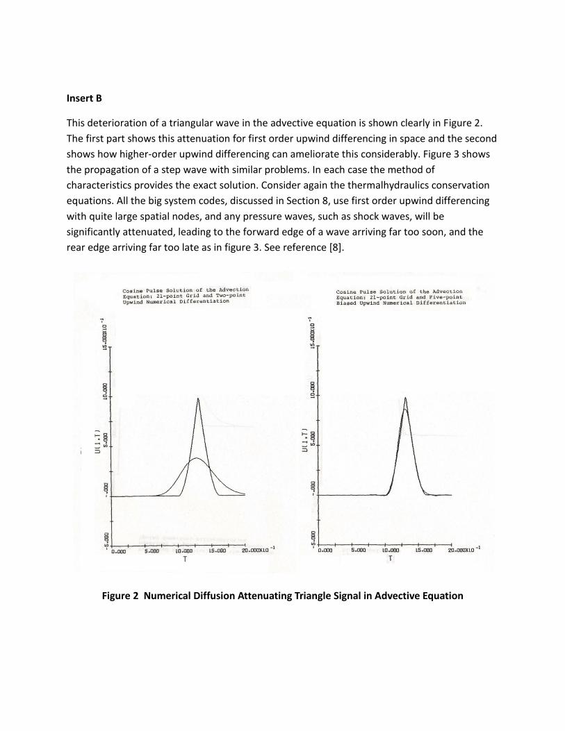
Insert B

This deterioration of a triangular wave in the advective equation is shown clearly in Figure 2.

The first part shows this attenuation for first order upwind differencing in space and the second

shows how higher-order upwind differencing can ameliorate this considerably. Figure 3 shows

the propagation of a step wave with similar problems. In each case the method of

characteristics provides the exact solution. Consider again the thermalhydraulics conservation

equations. All the big system codes, discussed in Section 8, use first order upwind differencing

with quite large spatial nodes, and any pressure waves, such as shock waves, will be

significantly attenuated, leading to the forward edge of a wave arriving far too soon, and the

rear edge arriving far too late as in figure 3. See reference [8].

Figure 2 Numerical Diffusion Attenuating Triangle Signal in Advective Equation

Insert B continued

Figure 3 Numerical Diffusion Spreading Shock Wave in Advection Equation

-11 -

In the second form of the momentum equation (30), the pressure term has here been extractedfrom the stress tensor so that the modified stress tensor now has only viscous terms.

The right side of the energy equation (31) contains terms addressing energy input from,respectively, external heating, internal conduction, pressure work, gravitational work, andviscous dissipation work.

The rhythm of equations is better revealed by using cartesian tensor notation:

+ =0 (32)dt cbc,

dt dXj dr. l dXj

4.2 The Viscous Stress Terms

The most general form of the momentum equation is for the case of a compressible fluid withvariable viscosity. For the simpler case of an incompressible fluid, the modified stress tensorbecomes:

x3i» <-\ / ^t i fj\* \

(35)dx. dXj

It is clear that - for most applications the momentum field will be stronglyinfluenced by the stress terms; and,

- these terms are quite complicated.

In computational fluid dynamics (CFD) of three-dimensional laminar flow, it is sufficient toinclude the molecular viscosity in the above terms. For successful simulation of turbulentflows the molecular viscosity is insufficient; instead, an effective turbulent viscosity is oftenintroduced, defined by

V^+V (36)

- 12-

A major part of the field of CFD consists of formulating turbulent models that use auxiliaryPDE's to describe the generation, transport and dissipation of turbulent kinetic energy, andhence provide a characterization of turbulence effects within an effective turbulent viscosity.An introduction to turbulence modelling is given in [9].

The equations of aerodynamics are inviscid, and thus avoid this particular problem. One-dimensional systems neatly circumvent this problem by replacing the viscous terms with asingle term involving the friction factor. This has some implication on the classification ofthe equations, and will be discussed later.

4.3 Conservative and Transportive Forms

The conservation equations stated above are in conservative form. The transportive formof the momentum or energy equation is obtained by subtracting the continuity equation. Thegeneral transportive form of the three-dimensional momentum equations is often referred to asthe Navier-Stokes Equations:

U ' ~ U Y . srr r-i\"r7 "r^ . r-r ~ vrr» . ~S . rr ~T f'V?^

The transportive forms and the conservative forms of the equations are equivalent, providingall equations are satisfied. This remains true for equations that have been discretisedproperly; however, the transportive form is not valid if mass continuity is not preciselymaintained during the evolution of a solution. This subtlety is exploited in some numericalschemes by incorporating the mass equation in the momentum and energy equations onlywhen it leads to better convergence properties [10].

4.4 Equation of State and Physical Properties

The conservation equations above have four primary variables, and can be expressed in matrixODE form as

A (d$ldf)=B , Q>=iV,p,et,P]T , V=[u,v,wf (38)

where the B matrix contains all external sources.

For n dimensions, n<3, there are n momentum equations, and hence n+2 equations for n+3unknowns. The remaining fluid equation is the equation of state. This relates thethermodynamic properties of the fluid and may be in the form of an equation (e.g., for anideal gas) or in the form of a correlation or tables (e.g., steam tables).

- 13-

Unlike the conservation equations, the equation of state is particular to the fluid involved; thegeneral form may be written in terms of internal energy or enthalpy:

(39)

4.5 Alternative Forms of the Energy Equation

The energy equation may also be expressed using BJ or h as the primary variable. Thederivation involves both the mass and momentum Equation [9], but results in similar forms:

dt dt ot

The appearance of the additional time derivative of P in (41) leads to further numericalcomplications, as it introduces a fourth time derivative in the three differential equations.

4.6 Constitutive Relationships

If the B matrix in (38) contains m additional auxiliary variables, then m constitutiverelationships are required for closure of the equation set; i.e., to provide a set of n+3+mdefinitive equations for the n+3+m variables. The constitutive relationships describe thevarious processes through which the fluid exchanges momentum and energy with its containerand beyond. These are usually algebraic equations, as in the case of friction and heattransfer, but also additional PDE's may be coupled to the conservation equations, as in thecase of modelling heat transfer to and through structures, modelling the neutron kineticsequations, and modelling effective turbulent viscosity.

Most constitutive relationships have some form of nonlinearity in the primary variables, andthis exerts a strong influence on the convergence of any solution method.

5. ONE-DIMENSIONAL METHODS

Most of the system thermalhydraulics codes used for safety analysis solve the transient one-dimensional equations. This represents the variables by their cross-sectional average values,

- 14-

and their interaction with the surroundings are based on correlations involving bulk values.

5.1 Method of Characteristics

The method of characteristics is very useful, as it was established particularly to address thepeculiar feature of hyperbolic equations - the fact that waves are propagated alongcharacteristic directions. As noted above, the one-dimensional advective equation

du du n— +c—=0dt dx

(42)

merely propagates an initial condition along the x-axis at speed c. The method ofcharacteristics reveals the characteristic vectors of the conservation equations, and how toutilize these in a numerical solution.

Replacing the viscous terms by a friction correlation as discussed above, the one-dimensionalEulerian equations (29-31) can be expressed [11] in general conservation law form as:

dt ox(43)

p,P",pe/=[p,G,£,]r , B=u<b+[Q,p,pu] (44)

It is convenient to introduce the local speed of sound:

This leads to the primitive form of the Eulerian equations:

(45)

at(46)

where:

. ,upp.

, D=

u 0 1/p'

p M 0

pc2 0 u

(47)

- 15-

Finally, the matrix A can be reduced to diagonal form A by similarity transformation, whereA is the matrix of eigenvalues:

'—y+k B'—ty=/

dt dx(48)

u+c 0 0

0 M 0

0 0 u-c

pc 0 1

0 c2 -1

-pc 0 1

(49)

Equation (47) defines three characteristics, each having one equality that is to be maintainedalong each characteristic, for example:

dx— =u+cdt

du dppc— +^dt dt

du dp.— +^dx dx

(50)

Combining the two equations (50) leads to an ODE to be solved along the u+c characteristic:

du(51)

The method of characteristics computes value from finite-difference approximations to thethree compatibility equations thus obtained, and establishes the solution on a grid that evolveswith the solution (wave tracing). Unlike fixed-grid methods, this allows waves to propagatewithout diffusion, hence the method is regarded as attaining the best attainable accuracy. Themethod is primarily used in gas dynamics, but has also been adapted for two-phase flow [12].

Obtaining numerical solutions from the method consumes too much time for general use, andit becomes increasingly difficult as the flow model increases in complexity, so alternativesthat combine the characteristic approach with more general integration methods have beensought [8,13,14].

5.2 Characteristic Differencing and Boundary Conditions

The classic method establishes the characteristic nature of hyperbolic equations and defines apragmatic method of properly choosing differencing algorithms and of assigning boundaryconditions for alternate numerical methods.

For positive flow, the above set has two forward characteristics, u,u+c, and one backwardcharacteristic, u-c. Hence, the equations require two inlet boundary conditions, normally u

- 16-

and p, and one outlet condition, normally P. Also, should u change sign, the methodconfirms the fact that a boundary condition on inflow at the exit is then required.

Further, the method establishes that directional differencing formulae, rather than centraldifferences, are most appropriate for hyperbolic equations; hence most alternative methods usesome form of upwind differencing that takes account of the fact that signals are propagated inthe characteristic directions. First-order upwind (donor-cell) differencing of the advectiveequation (42) results in:

ox

,00

,c<0

Numerical diffusion can be reduced by using higher-order formulae, by adding artificialviscosity terms [10], or by using very small dx.

5.3 Explicit and Implicit Finite-Difference Methods

The equation set (43) can be solved explicitly by applying (10); however, the explicit solutionis restricted by its largest eigenvalue to the Courant stability limit:

(53)

The Courant limit can be relieved by using semi-implicit methods, and it is something of anart to choose which terms are to be assigned to the new time level n+1. As noted in section2.3, the choice depends on the strength of coupling. A useful choice is to recognize thecoupling between pressure, continuity and momentum, such that the mass equation is solvedin fully implicit form and only the pressure term in the momentum equation is semi-implicit.

This relieves the Courant time step limit to the fluid transit time; i.e., removes the acousticrestriction, c, from (53) to give the so-called Material Courant limit:

(54)

Returning to the general ODE methodology, the conservation equations (43) can be written inODE form, and the solution may be obtained from (18):

This is the basis of the Porsching method [15], which is used in many thermalhydraulic

- 17-

codes. The method is almost fully implicit and has no stability limit on time step if the fullJacobian J is used. Recall from section 2.3 that the Jacobian is a linear representation of thecoupling between variables, and an approximation to J can be used to employ (55) as apredictor corrector iteration. If J is neglected entirely, (55) reduces to the Euler explicitmethod and is subject to the Courant limit (53). Including only the derivatives associatedwith the mass equation and pressure in J relieves this restriction to (54). It is impossible toinclude all coupling in J, as the partial derivative linearises non-linear terms.

It is also difficult to include even a linearised form of the coupling inherent in the heattransfer equations appearing in the constitutive relationships, so normally either some iterationis required, or some penalty applies in the form of a time step restriction.

It is useful to express the conservation equations (43) in ODE form, to illustrate the coupling:

(56)

Equations (56) can be put in the Jacobian form (55) as follows:

i--dp

M

dp

6p

dFc dFc

dG dE

3F dF. M M _wM

dG dE

dFP dFFi-dG BE.

finop

ÔG

- 'J

\F]

p

[FE\

(57)

Utilising the equation of state, 8p=(9p/3P)5 P, gives:

dp dP dG

OP i—dG

dG

dFc

dE

dFM

dE

WEdE.

fiPU A

ÔG

«

FcV-

c*

in*

(58)

- 18-

This is an almost implicit set that can be integrated in time using P, G and E as statevariables. The inclusion of P is a practical choice, as it enables pressure-boundary conditionsto be properly introduced as characteristic theory dictates.

It is also instructive to express (56) in residual form (20) and use Newton-Raphson to derivethe equivalent matrix equation to (58):

G=pu (60)

6ÔF 3ÔF

dp OP dG

dP dG

dôF

dP

BE

Be

dG dE

ÔG L/t+1 ifc (59)

This is equivalent to (58), for the first iteration, as (j^m-i^, but the residuals can be used asacceptance criteria for convergence. Further, if sufficient terms are included in the Jacobianderivatives, (60) can also be used for steady-state calculations.

A number of approximate forms can be used to reduce the size of the matrix solution to oneinvolving only one variable, usually pressure or flow. Examples of these methods arediscussed below.

5.4 Flow-Based Solution

The approach of reducing the matrix solution can be applied to equation set (57). In thiscase, the coupling to be considered is:

6Fr dFri- - 0dp dG

WM . 3FM dFM

dp dG dE

dFE dFE0 i-dG dE

00u p

ÔG

f\F(jj-j

FC\

FM

L E\

(61)

In this case, Porsching et al. [15] noted that the mass and energy equations can be solved

- 19-

algebraically in terms of the flow matrix:

BFf[op] = AïCtFcK-

(62)dFc

Equations (62) may now be substituted in (61) to give a single matrix equation for 5G:

dFM BF— c —Op OC7

0Cr

The final form is more complex as the pressure terms enter (63) through the derivative terms:

^=^M+^MdPdp_+^M.dP_dE_ (64)3G 3G 8P 9p dG dP 3E ÔG

Any constitutive relationships can also be linked via Jacobian terms. Porsching developed arigorous definition of the above methodology for piping networks, using a node-link grid inwhich scalars are defined at nodes, and velocities are defined in links joining the nodes.

5.5 Pressure-Velocity Solution

The large group of numerical methods generally classified as pressure-velocity (PV) methodswere originally developed for multi-dimensional analysis, but are also widely used for theone-dimensional equations. The well-known ICE [16] and SIMPLE [17] methods are theearliest variants of the PV theme, and use a staggered grid, in which scalars are defined atcontrol volume centres, and velocities are placed on the boundaries. Although expresseddifferently, the methods are much the same [18]. In one dimension, the staggered grid isidentical in concept to the node-link approach used in the flow-based solutions.

The PV methods were developed to recognize the fact that although the conservationequations in conservation-law form have four primary variables, they are governed by three

-20-

differential equations (56) and the equation of state (39). Although pressure is the drivingvariable, it is not computed from the differential equations, but enters the equations in asecondary manner through the equation of state.

This can lead to difficulties in handling boundary conditions if the equations are posed as astandard ODE set. The PV methodology circumvents this problem by re-establishing pressureas the driving influence. The simplest form can be illustrated by restating (60), and assumingweak coupling between the energy and the mass/momentum set:

ÔÔFcôp ÔÔFC '

op dP dG

KFM SWj, 0

9P dG

dOFEo nu uBE

OP

ÔG

OF,

= - OFM

OF,

(65)

Starting with an assumed pressure field, first estimates of G, and the relationship between ÔGand OP can be obtained by solving the momentum equation alone with oFM=0:

3ÔFMÔP+-

8ÔFM OG=0 (66)

Then, solving the mass and momentum equations together, as above, gives an equation inpressure correction alone:

dp dP BG BP dG[ÔP]= -ÔFC

(67)

Having solved (67), mass flows are now corrected using (66) and the energy equation is thensolved using the updated values of G and P; finally, density is computed from the stateequation. The sequence is iterated to re-establish the coupling to the energy equation.

If the Jacobian terms are applied to (44) in a simple manner that ignores second-order terms,Equation (67) becomes:

-si-'i t l & P i - ™ Af(68)

-21-

This is a wave equation for propagation of pressure at sonic velocity. Foi incompressible,flow, or steady state, it is a Poisson equation.

For two-phase flows, the energy coupling is often strong enough to require coupling to thepressure correction equation. This can be done in a similar manner, defining additionalcoupling in (65) through the equation of state:

aôFcap ÔÔFC BôFcdp

dp dP dG dp BE

dàFM daFM

dP dG

ôôF, 8ÔF-0 £ £

dG dE

OP

ÔG

OF,.

= -

OFC

W*

oF£

(69)

Then solve the energy equation for E, with OFE=0, and derive the relation between 8E andoG, and substitute this along with (66) into the mass equation, to get the pressure correctionequation:

dp dP dGdp a# dG

dp dEdG dP.[ÔP]= -ÔFC

(70)

Equation (70) is then used to update P,G,E and p. Some iteration is still required.

5.6 The Control Volume Equations

Equations (32-34) can be integrated over the control volumes, using Green's theorem, to givethe finite control volume statement of the equations; e.g., for the mass equation (32):

d(pV)/dt=(puA)M-(puA)out , V=fAdxi.e. (71)

dM/dt=Winl-Wc out ' M=pV , W=puA

The finite control volume method is basically the simplest form of finite-element method, asit uses a unit weighting function in the integration.

- 2 2 -

6. THREE-DIMENSIONAL METHODS

The one-dimensional equations can be solved as a set of shmiltaneous ODE's by some of theabove methods, but this is not always practical, and for multidimensional problems thematrices become unwieldy. It is more practical to use segmented methods that, like the lattermethods discussed, seek solutions by setting up matrix methods that solve one conservationequation at a time, and then incorporate the inter-equation coupling by iteration.

6.1 Pressure-Velocity Methods

Most multidimensional algorithms are based on some form of P-V algorithm. Multi-dimensional P-V algorithms are intricate and precise; however, the general approach isequivalent to Equations (65-67) and may be expressed [19] as follows.

The 3-D momentum equations with source terms, S, may each be discretised for coordinatedirection, i, at the point, xs, with respect to the other coordinates, j, and a previous time, t°:

(A*),- ' (72)

downstream ' upstream

If an initial pressure field, P, is assumed, each component of (72) may be linearised andintegrated over the control volume, to give

ai(pv)i=SJIfcJI(pv)B+c{(PD-/'^+<lZ>f , <R>i=!SdV=-I!ISjdxdydz (73)

where n is an index of each neighbouring control volume in each coordinate direction. Thismay be solved as a linear matrix equation for a new estimate of the mass flux matrix, [pv].

Integrating the mass equation and solving, using the [pv] matrix, resulting from (73) will ingeneral leave a non-zero residual Dr, such that:

- 2 3 -

The change in the pressure field to drive D to zero may be determined by Newton Raphson:

--D (75)dP

An expression for ÔD; is obtained by differentiating (74) and (73):

Kn

,) =~D. (76)

and

ÔP)] (77)

Equations (75-77) can be arranged into a matrix equation for the pressure correction field in aform that is the three-dimensional equivalent to Equation (68):

A OP = -D (78)

Once (78) is solved, the resulting pressure correction matrix can be used to adjust the massflux matrix by applying (77), and the procedure iterated to convergence for the time step.The method can be used as defined for homogeneous two-phase flow, and can be generalisedto two-fluid flow [19].

For heated systems, the usual practice is to solve the energy equation subsequent to the PViteration; however, the strong coupling between energy and momentum requires that theinteraction be catered for by also iterating around the PV-Energy sequence. Extensionsequivalent to the sequence (69-70) can also be derived.

6.2 Under Relaxation

Because segmented methods seek solutions to one conservation equation at a time, the outeriteration to address the inter-equation coupling may not converge. It is normally necessary toincorporate some form of relaxation. For example, the two coupled equations:

AX=B(X,T) , CY=D(X,Y) (79)

should be solved simultaneously, but could possibly be solved first for X, then for Y andrepeating the sequence; the fact that Y changes with X and vice-versa is neglected, and this

-24-

may inhibit or destroy convergence.

Convergence can be improved by introducing relaxation factors. For example if the vectorXm is returned from the m"1 iteration of the first equation, then a relaxed vector X™1 is sent tothe second equation:

(80)

The second equation is similarly relaxed using a 7^ Judicious choice of A* and Xy willimprove convergence. In applying (79), however, some of the coupling in X inherent to thefirst equation may now have been destroyed. It is more efficient [10] to modify the matrixequation to return a pre-relaxed value by building (80) into the matrix equation and solving:

Z7 x"rr=B(x)Y)-A7/ , ~Â'=Âh , 1"=-1(1 -Y^VY (81)

6.3 Numerical Diffusion

Numerical diffusion is omnipresent in three-dimensional computation, and is harder to control,because it no longer suffices to just take higher-order differences in the coordinate directions.It is necessary to "upwind" the differentiation in the characteristic direction of the flow, amethod that has come to be known as "skew upwinding" [20].

6.4 Alternate Coordinate Systems and Porous Medium Representation

Only rarely does the geometry of a physical system fit a standard coordinate system; hence aneed for more general methods arises.

Nuclear systems are often characterised by cylindrical vessels containing an array of tubes.Alternate ways of modelling such vessels are reviewed in [21] and [22], and include:

Subchannel Coordinate System - in which the equations are written for subchannels inside afuel bundle defined by imaginary Unes joining fuel-element centres. This reduces acylindrical (z,r,6) coordinate system into a (z,Q system, where Ç is a coordinate defining theimmediate neighbours to each subchannel. Since only first derivatives in the Ç direction canbe taken, correlations must be used for diffusion terms.

Porous Medium Representation - in which the equations are written in full 3-D form, butthe internal hardware is catered for by using a matrix of known porosity fractions, P, thatrepresent the fraction of each control volume available to the fluid (i.e., not occupied by thehardware). The porosity J3 is included in the equations simply by replacing p by Pp.

Insert C

Figure 4 shows a simplified (quarter-circuit) diagram of a representative CANDU Reactor

system.

Insert D

In Figure 4. these include the fuel coolant channels, the Steam Generator and the Calandria

Vessel.

Figure 4 Simplified (quarter circuit) Diagram of CANDU Reactor Components

Insert E

Figure 5 shows how a CANDU fuel channel can be modelled using subchannels.

Figure 5 Definition of Subchannel Geometry in a CANDU Reactor

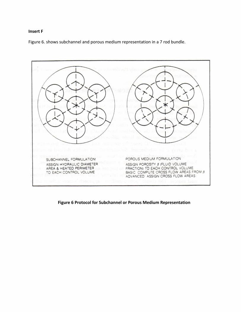
Insert F

Figure 6. shows subchannel and porous medium representation in a 7 rod bundle.

Figure 6 Protocol for Subchannel or Porous Medium Representation

-25 -

Arbitrary Coordinate Systems - the equations may be written in general orthogonal or non-orthogonal coordinates that are then deformed to fit the geometry. This body-fitted method isnow used in most commercial CFD codes. However, the mathematical implications arebeyond the scope of the current discussion; see [21] for an introduction.

7. TWO-PHASE FLOW EQUATIONS

7.1 Homogeneous Equilibrium Model

The homogeneous or equilibrium model of two-phase flow requires considerably moreconstitutive relationships than the single-phase case, but can be handled by any of thenumerical schemes already discussed. In this model, the two phases are assumed to be fullymixed such that they have the same temperature and velocity. The conservation equations fora homogeneous mixture are the same as for a single fluid, but require the extension of theequation of state to define saturation lines and two-phase quantities, and additionalconstitutive relationships to describe two-phase friction and heat transfer, and to define therelationship between weight and volume fractions, x and a. An overview of the model canbe found in [23].

7.2 Extended Homogeneous Model

Some non-equilibrium features, such as the effect of subcooled boiling on heat transfer,density and pressure drop, and the effect of unequal velocity (slip) on density and pressuredrop, can be added to the homogeneous model by means of additional algebraic equations,while still retaining the homogeneous conservation equations [23].

7.3 Non-Equilibrium Models

Non-equilibrium models of increasing complexity are obtained by introducing non-equilibriumeffects individually. A non-equilibrium model utilises individual conservation equations foreach phase. This permits the model to better approximate the general mechanics of a two-phase flow, hence it can better capture observed behavioral trends; however, many moreconstitutional relationships are now required to describe the factional and heat transferexchanges between the phases, and from each phase to the container. The state ofdevelopment of such constitutive models is still behind that for equilibrium models, soconsiderable uncertainties still exist. To minimise these uncertainties, various intermediateforms of the non-equilibrium models have been utilised.

The equal velocity unequal temperature (EVUT) model permits the phases to have unequaltemperatures, and hence requires two energy equations, one for each phase; see [13] fordetails.

- 2 6 -

The drift-velocity unequal temperature model (DVUT) adds another degree of freedom, byintroducing individual phase velocities through a full-range drift-flux model. This nowrequires a further conservation equation; usually, the mixture mass continuity equation isreplaced by one equation for each phase.

Finally, the full unequal velocity unequal temperature (UVUT) (two-fluid) model requires anindividual mass, momentum and energy equation for each phase, and more constitutiverelationships than one might at first realize.

The general statement of the equations must now involve some additional concepts. First, theassumption of interpenetrating continua [24] permits conservation equations to be written foreach phase as if each phase itself operates as a continuum interacting with another continuousphase, even under conditions such as bubbly flow and separated flow. Second, interactionsbetween the fluid are described in terms of an interface, which must have some interfacialarea, the définition of which is not inherent in the conservation equations, but requires furtherconstitutive equations that vary with flow regime.

Various forms of the two-fluid equations are discussed in [24], and the general statementbelow can be seen to be an extension of Equations (29-31) written for two fluids (or twophases), k&l, as follows:

ot oxt

(82)

(83)

(84)

The additional term in the mass equation is due to phase change. The additional terms in themomentum equation involve the pressure difference and shear stress between the fluids k&l,momentum transferred by phase change, and finally, a virtual mass term. The extra terms

Insert G

Figure 7 is a table showing which constitutive relations are required for each level of model

from EVET through to UVUT.

Figure 7 Constitutive Relations Required for EVET,UVET......UVUT Models of the Conservation

- 2 7 -

appearing in the energy equation are analogous.

Additional constraints exist, in that the phase volume fractions must sum to unity, and theinterphase relationships must be complementary, such that the individual phase equations,when added, return the standard mixture equations.

The above equations are stated as one set of conservation equations for each fluid, and manynumerical solution schemes solve them in this form; however, other options can be exploited.

For example, the equations can be added and subtracted, such that the working equations tobe solved are three mixture conservation equations and three equations expressed either interms of differences, or describing one fluid only. Another approach is to resolve the twomass and two energy equations into a mixture mass equation and three energy equations (themixture and each phase) [25]. This device adds the capability of considering options thathave only liquid disequilibrium or both liquid and vapour disequilibrium. The use of mixtureequations as one component part of the working equations can reduce the uncertainties indefining momentum and energy exchange between the phases from each phase to thesurroundings, by using traditional mixture correlations for both momentum and energy, andthen partitioning the energy and momentum transfer in the companion set of equations thatcaptures the departure from equilibrium. This approach is used to provide options forchoosing various levels of disequilibrium model in the ASSERT subchannel code [26], andthe TUF system code [27].

Finally, it is often important to include the presence of any non-condensable gases in thesolution, as they share the available flow area with the coolant. These are usually accountedfor by a transport model that assumes they travel at the same speed as the vapour phase;hence it usually suffices to solve an additional differential equation expressing massconservation of incondensables. However, an additional energy equation may be needed.

7.4 Numerical Solution and Hyperbolicity

As noted above, the inviscid equations are hyperbolic, and viscous terms in the one-dimensional thermalhydraulic equations are usually replaced by a correlation for factionalpressure drop; this renders the equations hyperbolic according to the above classificationschemes. The equation system must have real eigenvalues to be hyperbolic. Certain forms ofthe two-fluid equations, particularly those with a single pressure, generate complexeigenvalues, which give the equations a partially elliptic character that results in an ill-posedinitial-value problem. Some models choose the form of the virtual mass term and/or artificialviscosity terms, in a manner that ensure the equations remain well-posed (hyperbolic) duringthe evolution of the solution. The implications of hyperbolicity are still under debate [28].

While most 1-D two-fluid codes formulate the model in terms of Equations (82-84), and solvethem in a semi-implicit manner, using a staggered grid, many differences have evolved in the

-28 -

precise formulation, the choice of prime variables, the appropriate differencing of theequations and the choice of implicit terms. Particular codes are discussed in the next section.

7.5 Two-Step Methods

As mentioned above, even schemes that are designed to maximize implicitness are oftensubject to some time-step limit, due to numerical instability arising from the coupling ofauxiliary systems in a manner that cannot be easily captured in the linearised Jacobianderivatives used to represent the local variation of constitutive relationships and of theequation of state. Some causes of such instability have been found to relate to a number ofphenomena, such as: phase transitions that cause discontinuities in constitutive relationships,the progression of phase transition fronts though a finite grid system (water packing), or flowreversals that affect donor logic in the linearised terms and hence may deteriorate mass andenergy conservation.

A number of two-step approaches have been proposed, that basically work as two-steppredictor-correctors. Mahaffy [29] first used the two-step label for a predictor-correctormethod involving a predictor step and a stabiliser step. The scheme was devised for the two-fluid equations, but also applied to homogeneous flow. This method is too involved to detailhere. A simpler stabiliser step was proposed by Ransom [30], in the form of a subsequentmass correction equation that compensates for the difference in mass conservation caused bylinearisation in the linearised implicit solution.

7.6 Three-Dimensional Methods

Again, three-dimensional methods generally follow one of the two principal PV variants[16,17]. The principle is much the same, except that the presence of two fluids increases thedegrees of freedom that can be explored. The momentum equations may be formulated as(74), to provide an estimate of each velocity component, i, for each fluid, k, and differentiatedas in (77):

à ) ] (85)

The mass equations can be formulated to arrive at two residuals, Dk and DI} for fluids k and 1.

'•^ "' ^ " i• . TI rf A -. _..\ /"/(.. _..\ i _ r> (86)

The change in pressure is sought to drive the residual of the mixture mass equation D=to zero:

OD=S, 7 i + S y [ ( ^ a p v)D-(A a p v)^. (87)

Insert H

Figure 8 shows the scalar and vector control volumes required for a cartesian coordinate

system.

Figure 8 Staggered Grid Showing Scalar and Vector Control Volumes for 3D Cartesian

- 2 9 -

Hence a pressure equation similar in form to (78) is solved:

A ~aP=-D=-[Wk+'Dl\ (88)

and velocities are updated via (85). For fluids with widely disparate density, it can beadvantageous to base the pressure equation on a volumetric continuity, as below:

ÔD'-S, (89)

The question of an equation defining the volumetric fraction has been addressed in manyways. One continuity equation can be used; however, it is better to use an equation that isimplicit in both fluids. The IPS A method [31] is one option, and a simpler method with thesame degree of implicitness can be formulated by subtracting the two volumetric continuityequations, to give a second linear combination [19]. This gives:

^ ^i = 0 (90)

Having new values for the flow field variables, the energy equation can now be solved, andthe sequence is iterated. For boiling flows, improved coupling between energy and densitymust be established.

8. COMPUTER CODES FOR TWO-PHASE FLOW ANALYSIS

The following summarises the features of the principal computer codes used in analysis ofCANDU1 thermalhydraulics.

8.1 One-Dimensional System Codes

System codes have the capability of modelling flow and heat exchange in all components ofthe reactor coolant circuit, and its interaction with the rest of the system, including theneutronic feedback, fuel, pressure-tube, calandria tube, and the control system.

While it is possible to model each reactor channel, channels are usually analyzed inrepresentative groups. Most of the coolant circuit is in single-phase flow; however, normal

CANDU: CANada Deuterium Uranium; registered trademark.

- 3 0 -

operating conditions permit some void generation in the fuel channels, and postulatedaccidents considered in safety analysis invariably lead to transients causing significant voidgeneration, so all system codes need two-phase capabilities.

8.1.1 Two-Phase Codes

NUCIRC [32] is a steady-state system code used primarily in the analysis of critical channelpower. NUCIRC has an equilibrium flow model, modified to account for subcooled boilingand slip, and their effects on void and pressure drop. NUCIRC has the capability to modelthe whole coolant circuit and can simultaneously model all the individual reactor channels.

SOPHT [33] is a transient system code and uses an equilibrium flow model, modified toaccount for subcooled boiling and slip, and their effects on void and pressure drop. SOPHTmodels all components in the circuit. The numerical solution algorithm follows the PorschingFlow-Based approach.

FIREBIRD [34] is a transient system code and uses an equilibrium flow model, modified toaccount for subcooled boiling and slip and their effects on void and pressure drop. It hassimilar capabilities to SOPHT.

SPORTS [35] was written specifically for transient analysis of two-phase flow in low-pressurepool reactors. It solves the extended homogeneous equations using an iterative implicitmethod. Although the neutron kinetics equations are solved in a semi-implicit manner inmost system codes, work with SPORTS revealed that at low pressures these equations mustalso be treated fully implicitly, to avoid numeric oscillations [36].

8.1.2 Two-fluid Codes

RELAPS is often referred to as a standard of comparison, and has been occasionally used inCANDU analysis [37]. RELAP5-Mod2 [30] uses the full six-equation model, with a singlepressure and primary variables [v,,vg,eis,eu,P,ag]. Individual phase pressures are extracted forstratified flows. Two options are available to avoid the material Courant limit: a semi-implicit two-step method, and a "nearly implicit" method that provides the maximum possiblecoupling available for the linearised equations. For the two-step method, the mass andmomentum equations are first resolved in an implicit PV formulation, and then the energyequations are arranged in the semi-implicit form of (55), where [0] is [P,ag,eig,ej,], and solvedfor the time step, using property derivatives based on the state equations, to provide thelinearised (Jacobian) terms wherever possible.

CATHENA [38] uses the full six-equation model with two pressures, giving seven principalvariables, which are reduced to six, [v1,vg,hg,hli,P,ag], by using a constitutive relationship forinterphase pressure difference. These are arranged in the semi-implicit form of (55), againwith property derivatives used in supplying the Jacobian terms, and the resulting linear set is

-31-

solved in the time step by a sparse matrix package (the saine package as in [6]). Astabilising corrector step based on mass conservation is applied. Time-step control is basedon considerations of the rate of change of variables.

TUF [27] uses a full six-equation model with principal variables [Mm,Mg,Em,Eg,Wm,vr]. Thesolution method is a two-step method with an explicit predictor step and an implicit step thatis a two-fluid extension of the Porsching flow-based method. TUF includes options forvarious levels of departure from equilibrium (sse section 7.3).

All three of the above codes include equations for non-condensables.

8.2 Multidimensional Component Codes

Multidimensional analysis is not widely used in system codes, because of the increasedcomplexity and expense of multidimensional solutions, but some multidimensional auxiliaryfeatures are often used (for example, conduction in the fuel model).

In general, multidimensional codes concentrate on particular components, such as the channel,steam generator, calandria, etc.

The ASSERT subchannel code [26] was written 'o model two-phase flow in the horizontalfuel channels of CANDU reactors. It uses the DFUT model, which allows the phases to haveunequal temperatures and velocities. The definition of subchannel is the same as that used inCOBRA-IV [39]; however, COBRA-IV uses the equilibrium model of two-phase flow.ASSERT has an equilibrium option that permits it to solve the same equations as COBRA-IV,but the nonequilibrium options permit ASSERT to mechanistically model the onset ofsubcooled boiling in particular subchannels, and the resulting redistribution of flow amongstthe subchannels, and the progression towards stratification that occurs in horizontal channelsat higher void fractions. ASSERT is used primarily in steady-state for analysis of criticalheat flux (CHF) for various flow conditions, particularly in the case of variations of fluxprofile or pressure-tube geometry that are beyond the experimental data on CHF. The codealso has the capability to do transients involving post-dryout and flow reversal; however,three-dimensional transients are expensive.

The THIRST code [40] is for analysis of the thermalhydraulics of steam generators.THIRST solves the extended homogeneous equations on a three-dimensional grid to obtainthe distribution of flow and phases in the secondary (shell) side of a recirculating steamgenerator. Temperatures of the primary (tube) side is also computed, together with acalculation of recirculation ratio and steam production. Apart from analysis of steam-generator performance, THIRST is also used to compute local flow velocities and voidfraction that are required as input for calculation of the vibration and wear of the tube arrays.An auxiliary code, SLUDGE [41], provides a calculation of the distribution and deposition offouling matter within the steam generator, given the velocity fields from THIRST.

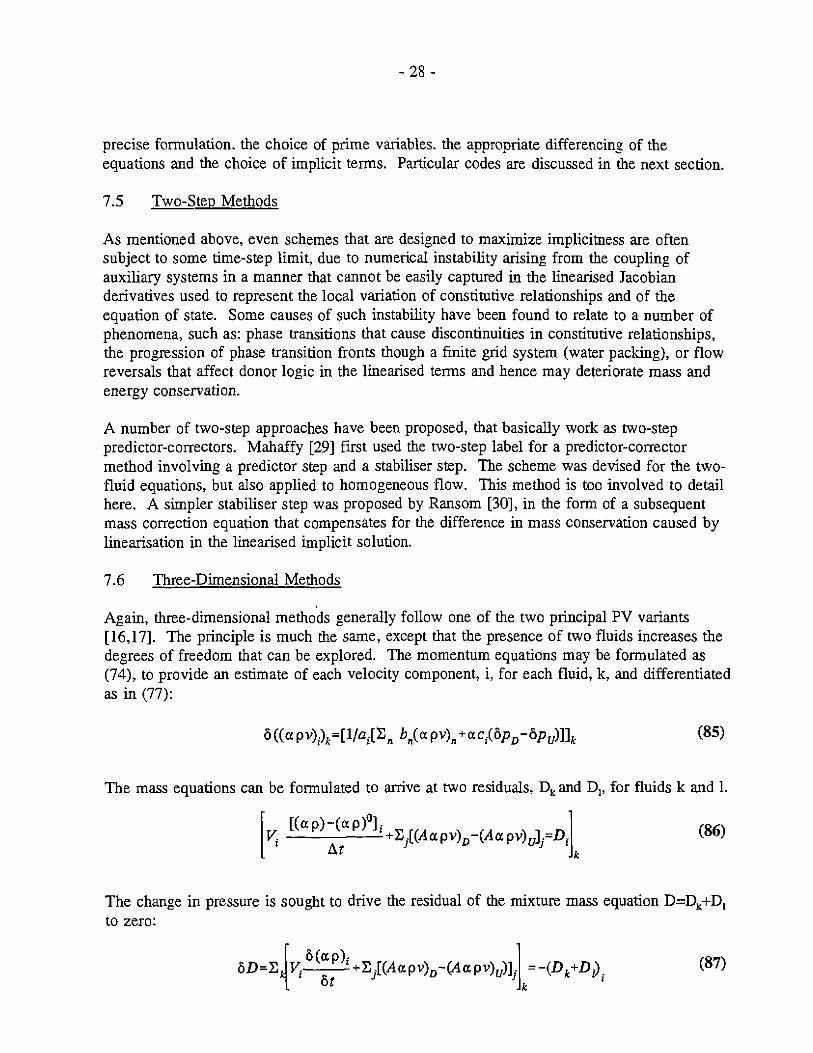
Insert I

The codes above all use a one dimensional model - z - of the coolant flow, but the complication

of the data description is immense; Figure 9 shows a nodalisation for Darlington 4 [50]. The

codes compute rod surface temperatures at location 'z'. Because the power profile in a bundle

is non- uniform, it is possible to estimate surface temperatures of selected rods, particularly the

hottest rod (the one with the highest power generation). Users should be aware that the actual

hot rod temperature will be higher because flow distribution must de facto be neglected. Figure

10 shows some results from SOPHT [33,50].

Figure 9 SOPHT nodalisation for Darlington 4

Insert I continued

Figure 10 LOCA, SOPHT: Hot Element Power Transients for Inlet Header Breaks, Menely[50]

Insert J

Figure 11 shows an ASSERT study of the effect on CHF of pressure tube creep. The measured

and modelled locations of dryout are shown for an electrically simulated CANDU bundle.

Figure 11 ASSERT Study of Effect of Crept PT on CHF

Insert J continued

Figure 12 shows a MAPLE X10 fuel channel with numbering for rods and subchannels.

Figure 12 MAPLE X10 Fuel Channel with Numbering forSubchannels and Fuel Rods

Insert K

Figure 13. shows THIRST analysis of a steam generator secondary side flow using the porous

medium approach to incorporate the hardware of the secondary side ( a complex arrangement

of inverted u-tubes with many stabiliser bars and a pre-heating heat exchanger).

Figure 13 THIRST Study of Steam Generator Thermalhydraulics

-32-

8.3 Commercial Codes

Significant advances in CFD methodology in arbitrary coordinate systems, combined with theincreased complexity required to incorporate these advances, has gradually removed the fieldfrom the realm of the general practitioner to that of the focussed specialist This trend hasspawned a significant increase in the number of advanced CFD codes offered on acommercial basis. Most of these codes are not sold on a black-box basis, but rather togetherwith a certain amount of consulting support from the parent company. The performance ofthe codes for single-phase flow is well established, and their accuracy is primarily a functionof the applicability of the turbulence model used. Usually, the codes contain a choice ofturbulence model, thus shifting that responsibility to the user. We mention three here thathave been used in analyses related to CANDU.

TASCFLOW [42] is a single-phase, three-dimensional CFD code for arbitrary geometries,offered by ASC. It has been applied successfully to very complex geometries. An earlyversion of TASCFLOW forms the basis of the MODTURC program, that models moderatorflow in CANDU calandrias [43]. TASCFLOW has also been used in modelling flow inconduit junctions [43], and past spacers in CANDU, fuel bundles in order to quantify theassociated heat-transfer enhancement [44].

PHEONICS [45] is another three-dimensional CFD code for arbitrary geometries, written byCHAM; and has also been used for analysis of calandria flow [46]. PHEONICS advertises afairly extensive two-fluid option.

FLOW-3D [47], a three-dimensional CFD code for arbitrary geometries, from CFDS, also hasa two-fluid option. FLOW-3D has been applied to the analysis of pool reactors [48], and tomodel void distribution in channels [49].

9. CONCLUDING REMARKS

The preceding has reviewed the current state of numerical methods for solution of thethermalhydraulic equations. Most of the methods currently in use have their roots innumerical methodology that was developed in the 1970's and was hence focussed on thecomputing capabilities of that era, when limitations on available memory led to an emphasisof segmented methods over direct methods. As today's computers are not subject to suchstringent storage limits, the trend in CFD software is towards more direct methods thatmaximize coupling, leading to significant reduction in the convergence problems that oftenhamper the segmented methods.

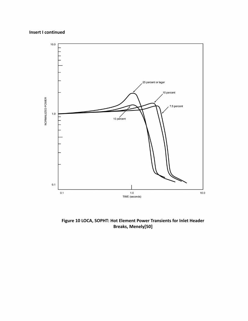
Insert L

Figure 14 shows results of TMODTURC 2D modelling of flows inside a CANDU calandria [43].

Figure 14 Pickering Calandria Experiments a>Simplified Front View b> Computed

Insert M

In such computation it is necessary to use some form of turbulence model for a two fluid

system; this is easiest to address in bubbly flows such as [49] as one can legitimately state that

the near wall turbulence is dictated by the continuous fluid and there is evidence that this does

work fairly well for bubbly flows[19,51]; the technique is described in detail in [52].

FAITH [19] is a 3D @ Fluid CFD code developed by the author; it is not commercially available.

Figure 15 shows computed redistribution of air and water in the Ecole Polytechnique

subchannel experiments[53]. Finally Figure 16 [19]shows the fascinating redistribution of air

and water in a vertical pipe, through a 90 degree bend to a horizontal pipe.The phases go

through a complete swap as centrifugal acceleration moves the water radially until it is driven

back by gravity in the horizontal section.

Insert M continued

Figure 15 FAITH code Simulation of Air-Water Redistribution in

Insert M continued

Figure 16 FAITH code Simulation of Air-Water Redistribution in

- 3 3 -

10. ACKNOWLEDGEMENTS

The author thanks the following colleagues: A.O. Banas, Y. Liner, and R.Q.N. Zhou reviewedthe document and contributed suggestions, W.S. Liu forwarded background material on theTUF code, and DJ. Richards mentioned reference 37.

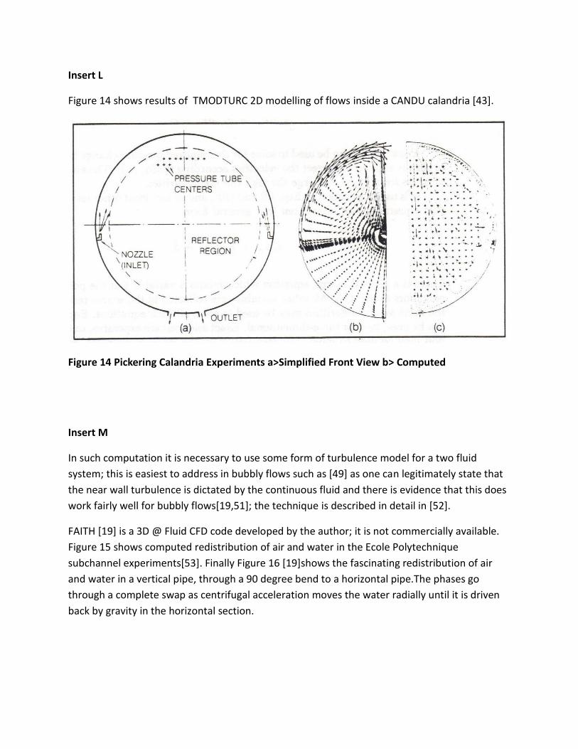
11. REFERENCES

[1] L. Lapidus and J. Seinfeld, "Numerical Solution of Ordinary Differential Equations",Academic, New York, 1971.

[2] W.E. Schiesser, "Computational Mathematics in Engineering and Applied Science -ODE's, PDE's and DAE's", CRC Press, Ann Arbor, 1994.

[3] W.E. Schiesser, "The Numerical Method of Lines Integration of Partial DifferentialEquations", Academic Press, San Diego, 1991.

[4] M.B. Carver, "Automated Solution of Arbitrarily Defined Partial and OrdinaryDifferential Equations, FORSIM Package, Theory and User Manual", AECL-5821,1978, also Computer Physics Communications, 17, 239-282, 1979.

[5] C.W. Gear, "Automatic Integration of Stiff Ordinary Differential Equations",Comm.ACM, 14, 3, 176-190, 1971, also "Numerical Initial Value Problems in OrdinaryDifferential Equations", Prentice Hall, Englewood Cliffs, NJ, 1971.

[6] M.B. Carver and S.R. MacEwen, "On the Use of Sparse Matrix Approximation to theJacobian in Partitioning Large Sets of Ordinary Differential Equations", Siam J. S ci.Stat. CompuL, 2, 51-64, 1981.

[7] B.P. Leonard, "A Survey of Finite Differences of Opinion on Numerical Muddling ofthe Incomprehensible Defective Confusion Equation", Finite Element Methods forConvective Dominated Flows, AMD v34, ASME, 1979.

[8] M.B. Carver, "Pseudo-characteristic Method of Lines Solution of the ConservationEquations", J Comp Phys, 35, 1, 1980, p57-75.

[9] D.A. Anderson et al., "Computational Fluid Mechanics and Heat Transfer",Hemisphere, New York, 1984.

[10] S.V. Patankar, "Numerical Heat Transfer and Fluid Flow", Hemisphere, New York,1980.

- 34 -

[11] R.D. Richtmeyer and K.W. Morton, "Difference Methods for Initial Value Problems inFluid Dynamics", Interscience, New York, 1957.

[12] W.T. Hancox and S. Banerjee, "Numerical Standards for Flow Boiling Analysis", Nucl.Sci. & Eng., 64, 106, 1977.

[13] DJ. Richards and B.H. McDonald, "Dynamic Grid Allocation for the CharacteristicFinite Différence Scheme", Proceedings, 3'rd CSNI Specialists in Transient Two-PhaseFlow, p433-448, Hemisphere, 1983.

[14] N.P. Kolev and M.B. Carver, "Pseudo-Characteristic Method of Lines Solution of theTwo-Phase Conservation Equations", Proceedings, 3'rd CSNI Specialists in TransientTwo-Phase Flow, p449-464, Hemisphere, 1983.

[15] T.A. Porsching et al., "Stable Numerical Integration of Conservation Equations forHydraulic Networks", Nucl Sci & Eng, 43, 218-225, 1971.

[16] F.H. Harlow, and A.A. Amsden, "A Numerical Fluids Dynamics Method for AllSpeeds", J. Comp. Phys., 8, 2182-2201, 1971.

[17] S.V. Patankar and D.B. Spalding, "A Calculation Procedure for Heat Mass andMomentum Transfer in Three-Dimensional Parabolic Flows", Int J Heat & MassTransfer, 15, 1787-1806, 1972.

[18] M.B. Carver, "Some Continuity Considerations in Multidimensional Two FluidComputation", Proceedings, 3'rd CSNI Specialists in Transient Two-Phase Flow, p341-352, Hemisphere, 1983.

[19] M.B. Carver and M. Salcudean, "Three-Dimensional Numeric modelling of PhaseDistribution of Two-Fluid Flow in Elbows and Bends", Num Heat Transfer, 10, p229-251, 1986.

[20] G.D. Raithby, "Skew Upstream Differencing Schemes for Problems in Fluid Flow",Comput. Methods Appl. Mech. Eng., 9, 153-164, 1976.

[21] W.T. Sha, "An Overview of Rod-Bundle Thermalhydraulic Analysis", Nucl.Fr.g &Des.62, 1-24, 1980.

[22] M.B. Carver, "Multidimensional Computational Analysis of Row in Nuclear ReactorComponents", Trans. Soc. for Computer Simulation, 1, 2, 97-116, 1984.

[23] R.T. Lahey and FJ. Moody, "Thermalhydraulics of a Boiling Water Nuclear Reactor",ANS, New York, 1975.

- 3 5 -

[24] M. Ishii. "Thermo-Fluid Dynamic Theory of Two-Phase Flow", Eyrolles, Paris, 197:5.

[25] S.W. Webb and D.S. Rowe, "Modelling Techniques for Dispersed Multiphase Flows"Encyclopaedia of Fluid Mechanics, Gulf publishing, Houston, 1986.

[26] M.B. Carver, J.C. Kiteley, D.S.Rowe, "Simulation of the Distribution of Flow andPhases in Vertical and Horizontal Fuel bundles using the ASSERT subchannel code",Nucl. Eng.& Des., 122, 413-424, 1990.

[27] W.S. Liu et al. "TUF a Two-Fluid Code for Thermalhydraulic Analysis", tenth CNSConference, Ottawa, 1989.

[28] V.H. Ransom, "Convergence and Accuracy Expectations for Two-Fluid FlowSimulations", Proceedings, 1990 CNS/ANS Int. Conf on Simulation Methods inNuclear Engineering, Montreal, 1990.

[29] J.H. Mahaffy and D.R. Liles, "A Stability Enhancing Two-Step Method for Fluid RowCalculations", J Comp. Phys., 46, 329-341, 1982.

[30] V.S. Ransom et al., "RELAP5-Mod2 Code Manual, Code Structure, Models andSolution Methods", NUREG/CR-4312, 1985.

[31] D.B. Spalding et al., "Calculation of Two-Dimensional Two-Phase Flows", Two PhaseFlow Momentum and Heat Transfer in chemical Processes, F. Durst, éd., Hemisphere,Washington, 1979.

[32] R.F. Dam et al., "ASSERT/NUCIRC Commissioning for CANDU-6 Fuel Channel CCPAnalysis", Proceedings, 1994 CNS Simulation conference, Pembroke, 1994.

[33] J.S. Skears and Y.F Chang, "A Thermalhydraulic System Simulation model for theReactor, boiler and Heat-Transport System (SOPHT)", Ontario Hydro Report,CNS-3-2, 1977.

[34] J. Ballyk et al., "FIREBIRD Comparison of Multi and Average Channel CircuitSimulation of a 20% RIH Break", Proceedings 17'th CNS Simulation symposium,Kingston, 1993.

[35] V. Chatoorgoon, "SPORTS a Simple Non-Linear Thermalhydraulic Stability Code",Nucl. Eng. & Des., 93, 51-67, 1986.

[36] V. Chatoorgoon, "Coupling of Thermalhydraulic and Neutron-Kinetic Equations forImplicit Schemes", Proceedings, Fourth BNES Conference on Dynamics and Control inNuclear Power Stations, London, p31-37.1991.

[37] S.H. Lee et al., "RELAPS Analysis of Large Break LOCA in CANDU System",Proceedings, Korean Nuclear Society, Autumn Meeting, p63-68, 1993.

- 3 6 -

[38] D.J. Richards et al., "(QATHENA a Two-Fluid Code for CANDU LOCA Analysis".Proceedings, third International Topical Meeting on Reactor Thermalhydraulics,Rhode Island, 1985.

[39] C.W. Stewart et al., "COBRA-IV, the Model and The Method", BNWL-2214, 1984.

[40] M.B. Carver, L.N. Carlucci and W.R. Inch, "THIRST - Thermalhydraulics inRecirculating Steam Generators, Users manual", AECL-7254, 1981.

[41] Y. Liner, M.B. Carver, C.W. Turner and A.O. Campagna, "Simulation of MagnetiteParticulate Fouling in Nuclear Steam Generators", ASME NE-Vol8, p!9-27, 1992.

[42] TASCFLOW Version 2.1 User Documentation, Advanced Scientific Computing,Waterloo, 1991.

[43] Y. Szymanski et al., "Spatial convergence of Flow Solutions in MODTURC-CLAS",Proceedings, 3'rd CNS/ANS Int. Conference on Numerical Methods in Engineering,Montreal, 1988.

[44] A.O. Banas, M.B. Carver and C.A. Whitehead, "Numerical Studies of Flow and Heat-Transfer around Fuel-Element Bearing Pads", Proceedings, 4'th CNS/ANS Conferenceon Simulation Methods in Nuclear Engineering, Montreal, 1993.

[45] D.B. Spalding et al., "Mathematical Models in Nuclear Reactor Thermalhydraulics",Proceedings ANS Topical Meeting on Thermalhydraulics, R.T. Lahey, ed, 1980.

[46] W.M. Collins et al, "Application of the PHEONICS code for Moderator SystemConditions in a CANDU Reactor", Proceedings, 3'rd Int. Conference on SimulationMethods in Nuclear Engineering, Montreal, 1990.

[47] CFDS-FLOW3D User Guide, Computational Fluid Dynamics Services Inc, 1992.

[48] M.B. Carver, S.J. Marshall and P.W. Shipp, "Application of FLOW3D to FlowModelling in Small Natural Circulation Pool Reactors", Proceedings, 3'rd Int.Conference on Simulation Methods in Nuclear Engineering, Montreal, 1990.

[49] A.O. Banas, M.B. Carver and D. Unrau, "Prediction of Bubbly Flow in Pipes UsingTwo-Fluid Models in CFDS-FLOW3D", Proceedings, 17th CNS SimulationSymposium, Pembroke, 1994.

Insert N

[50] Dan Meneley, Nuclear Safety and Reliability Course, Week 9, University of New Brunswick,Canada, October 2003, CANTEACH, https://canteach.candu.org.

[51] D.A. Drew & R.T. Lahey, Phase Distribution Mechanisms in Turbulent Two-Phase Flow, J.Fluids Eng., vol 103, 1981.

[52] M.B Carver, The Development and Application of Three-Dimensional Two-Fluid NumericalAlgorithm for Simulation of Phase Redistribution by Bends and Obstructions, PhD thesis,University of Ottawa, Mechanical Engineering, 1986.

[53] A. Tapucu & S. Gencay, Experimental Investigation of Mass Exchanges Between TwoLaterally Interconnected Two-Phase Flows”, Ecole Polytechnique, CDT project number P-533.

AECL-11387ARD-TD-550

Cat. No. /No de cat: CC2-11387EISBN 0-662-16235-0

ISSN 0067-0367To identify individual documents in the series, we have assigned anAECL- number to each.

Please refer to the AECL- number when requesting additional copies ofthis document from:

Scientific Document Distribution Office (SDDO)AECLChalk River, OntarioCanada KOJ 1JO

Fax: (613) 584-1745 Tel.: (613) 584-3311ext. 4623

Price: B

Pour identifier les rapports individuels faisant partie de cette série, nousavons affecté un numéro AECL- à chacun d'eux.

Veuillez indiquer le numéro AECL- lorsque vous demandez d'autresexemplaires de ce rapport au:

Service de Distribution des Documents OfficielsEACLChalk River (Ontario)Canada KOJ 1JO

Fax: (613) 584-1745 Tél.: (613) 584-3311poste 4623

Prix:B

Copyright © Atomic Energy of Canada Limited, 1995