multidimensional evaluation of regional plans serving multiple objectives

E L E V E N T H EUROPEAN CONGRESS OF THE REGIONAL SCIENCE A S S O C I A T I O N

MULTIDIMENSIONAL EVALUATION OF REGIONAL PLANS SERVING MULTIPLE OBJECTIVES

by Morris Hill and Yigal Tzamir*

1. INTRODUCTION

Plans for regional development characteristically serve multiple objectives. At its most literal, regional planning may be defined as a process for determining the optimal allocation of resources in order to achieve a set of objectives defined in space. This multiple objective characteristic of regional planning has, however, only re- cently become a focus of attention in the literature/ Such objectives may appear in a general or specific form. The extent of specificity of objectives reflects the existence of a hierarchy of goals in which lower level goals are the specification of means for achieving higher level goals. While higher goals may thus have in- trinsic value, goals at the other levels have instrumental value in that they are intended, explicitly, to lead to the achievement of the higher level goals relating to such issues as national or regional economic growth, income stability, income distribution, or enhancement of the environment? A second level may relate to such issues as population distribution or regional independence? A third level may be even more concrete relating to issues such as the relative location of regional activities, densities, accessibility, etc. The rational evaluation of plans for regional development requires the explicit choice of that regional development strategy which best achieves the preferred objectives. The evaluation process may be addressed to any of the levels in the goal hierarchy as long as the level is significant for the decision- making body. At each level, however, one is likely to be faced with the question of multiple objectives and the resultant necessity of comparing plans which differentially achieve the various objectives. In other words, a typical problem in the evaluation of regional plans is the existence of a multidimensional objective function which explicitly incorporates conflicts among objectives. The explicit recognition of a multiple objective function does not resolve these conflicts but only identifies them.

Given a multiple objective function, how might the optimal plan be chosen? If the objectives are not completely complementary (i.e., do not represent multi-

* The authors are associated with the Center for Urban and Regional Studies, Technion-Israel Institute of Technology, Haifa, Israel.

1 For early treatment of the subject, see Leven [10], see also Reiner [17]. 2 These objectives are the ones that are referred to in the U.S. Appalachian Regional Develop-

ment Act of 1965. a This is the level of objectives referred to in the Israel Physical Master Plan, see Dash and Efrat

[3].

140 PAPERS OF THE REGIONAL SCIENCE ASSOCIATION, VOL. 29, 1972

supporting sub-goals of the same higher-order objectives), it becomes necessary to develop a method of choice which incorporates the levels of achievement of the objectives by the alternative plans. In such a case, the simplest solution would be provided by lexieographic ordering, when one objective is assumed to be dominant. The plan which achieves this objective to the highest degree is, by definition, the optimal plan. Only when plans are equivalent in terms of the achievement of this objective do the other objectives come into consideration; see Steiner [18; p. 42] and Reiner [17; p. 277]. In the absence of either mutually supportive objectives or one dearly dominant objective, the evaluation process becomes considerably com- plicated. Then, the simplest case would occur when one of the alternative plans under consideration has a higher level of achievement of each of the preferred objectives than any of the other plans. Such a plan is clearly the optimal one. How- ever, the usual situation requires some method of aggregation of outcomes, measured in different units of goal-achievement, frequently on different classes of measurement scales. The need to aggregate the expected outcomes of alternative plans with respect to their achievement of objectives exists whether the planning process is sequential or cyclical; see Boyce, McDonald, and Day [2]. In all cases, the point of departure of this aggregation is the disaggregated statement of the achievement of objectives. In this disaggregated statement, the level of achievement of each objective by each of the alternative plans is explicitly stated, being expressed in the measurement units by which the achievement of the objective is usually measured. These units of measurement may be expressed on any of the possible measurement scales which are listed here by increasing order of measurement: nominal, ordinal, interval, and ratio? In Sections 2 and 3, two separate methods will be discussed by which aggregative evaluation may be accomplished.

2. AGGREGATIVE EVALUATION BY UNIFICATION OF MEASUREMENT SCALES

This approach involves the translation of goal variables into common units of measurement. It is a reasonable approach when a unit measure of goal-achievement can be established which incontrovertibly expresses the original scales according to which the objectives were measured. The aggregative choice can then be determined by a simple arithmetic procedure. There are several examples of this particular aggregative approach.

Cost-Benefit Analysis This is probably the most common method of plan evaluation and requires

the expression of the expected effects of the plan under consideration in monetary terms. Costs represent the monetary value of goods and services employed in the implementation of the plan while benefits represent the value of favorable outcomes resulting from the planned course of action (and which would not have occured without it). In practice, cost-benefit analysis is intended to measure the effectiveness of plans in contributing to national economic efficiency and, if various assumptions

4 For an extensive discussion on the measurement of goal-achievement according to measurement scales of different order, see Hill [6; pp. 24-25].

HILL AND TZAMIR: EVALUATION OF REGIONAL PLANS 141

are met, to national economic welfare. The method is most attractive in that it expresses the expected outcomes of plans in terms which are meaningful for budgetary officials and others having responsibility for proposing and reviewing the allocation of government resources. However, when cost-benefit analysis is employed as the only method of plan evaluation, it has serious drawbacks for which it has been severely criticized. First, whereas it purports to measure economic welfare (or even national economic efficiency), it really cannot do so because of the difficulty of measuring the economic benefit of collective goods and because of the impossibility of meet- ing the assumptions required by economic theory for the incontrovertible measurement of these objectives; see Krutilla [9]. Second, it neglects the effects on objectives which cannot usefully be expressed in economic terms (intangibles) or dis- torts the perception of the essence of such effects if they are so expressed.

Transformation Functions These represent another approach to the problem which, although promising,

has not been applied in practice and, as far as regional and urban planning is concerned, remains in the sphere of the conceptual; see Ackoff [1] and particularly Fishburn [4]. According to this approach, outcomes measuring the level of goal- achievement on one scale are expressed in equivalent levels of achievement on another scale. Thus, the level of achievement of one objective may be translated at all levels of achievement of another objective. There is no reason to assume linear relationships between the levels of achievement of two objectives, i.e., at one end of the scale, the value of achievement of x units of objective A may be considered equivalent to y units of objective B; however, at the other end of the scale, x units of objective A may be considered equivalent to z units of objective B. Cost- benefit analysis may be considered a particular case of the use of transformation function whereby all possible effects (including those affecting the achievement of other objectives) are expressed in terms of economic efficiency. A crucial difference, however, is the inherent linear assumption of cost-benefit analysis. The essential difficulty with the use of transformation functions is operationalizing them.

Weighted Index of Goals-Achievement This approach involves the expression of objectives in terms of quantitative

measures which reflect the extent of achievement of each objective. Each objective has its relevant index. Such indices have been developed for efficiency and equity objectives by McGuire and Garn [16]. Hill and Shechter [8] have proposed a set of such indices for the evaluation of plans for the development of outdoor recreation facilities. In the latter case, indices of achievement were developed which expressed the achievement of national economic benefits, regional economic benefits, distributional equity, preservation of natural areas, choice, and public par- ticipation. The indices of achievement of objectives are then summed for each alternative plan, a relative weight being applied to each. This procedure can be applied for the community as a whole and/or for particular sub-groups within the community. Indices can be normalized so that the method of measurement of the index does not provide an unintended weight resulting from the relative size of the


index. The advantage of this method of aggregation is that it provides an aggregate statement of outcomes, expressed in a neutral manner. (Unlike cost-benefit analysis, outcomes are not translated in terms of a single objective. ) It is, instead, a true aggregate of outcomes which affect the various objectives. The major criticisms of this approach relate firstly to the lack of popular understanding of the significance of an aggregate goals-achievement index, and secondly to the assumption of static linear weights. The latter criticism is not necessarily inherent in the method since it can be explicitly assumed that for certain ranges of goal-achievement (i.e., for certain ranges of value of the indices), the relative importance or the weight changes. ~ For instance, as income increases the marginal value of an extra dollar of income decreases, this being expressed by a non-linear weighting function.

3. AGGREGATIVE EVALUATION BY MEANS OF ACCOUNTING FRAMEWORKS

This involves the cooption of the decision-making body into the aggregation process. Such an aggregation procedure is based on the decision-makers' informed and reasoned judgement of information recorded in a balance sheet or goals- achievement account expressing the effects of the plans. According to this approach, the expected effects of the alternative plans are recorded for each relevant objective in a disaggregated form. The aggregation is left to the reasoned judgement of the decision-maker (who may also be the planner), without the aid of an objective technique in the aggregation process. This approach requires a greater active involvement of the decision-maker in the evaluation process than the methods previously discussed, and has several variants.

The Planning Balance Sheet This was developed by Lichfield [11] [12]. It records the advantages (benefits)

and disadvantages (costs) accruing to various homogenous sectors of the population from the alternative plans. These costs and benefits are recorded on a monetary scale, or, if this is not possible, on a quantitative non-monetary scale or, if this also is not possible, on an ordinal or nominal scale. The outcomes are then aggregated on a judgemental basis from the point of view of the effects on the various sectors. These aggregate judgements are stated in a reasoned manner for each sector and then for all sectors in the community, the explicit reasoning being subject to the decision-maker's review.

The Goals-Achievement Account This is akin to the planning balance sheet but the emphasis is on the explicit

identification of objectives, measured in their relevant units, with costs and benefits being the positive or negative effects of the plan on goal achievements; see Hill [6; p. 25] and Hill [7]. Each goal thus has its typical set of costs and benefits. The incidence of costs and benefits (i.e., goal-achievement) for various groups and locations in the planning region is also recorded. These outcomes are then corn-

For a non-linear weighting system, see Freeman [5].


pared by the decision-maker and/or analyst with the weights of the objectives for the community as a whole or for the various sections within it, and an aggregative

judgement is arrived at.

Goal Fabric Analysis This was proposed by Mannheim and Hall [15] as a goal-accounting framework

which, in part, employs the unification of scales to determine the preferred alternative. As a first step, all known goals are listed. The goals are then structured so that relations between them can be determined. This is done by one of several methods: identifying which goals are specifications of others; establishing meansends relationships and determining the goals which are (value-wise) dependent and (value-wise) independent. This analysis produces a hierarchical tree-type structure leading from the general goals to the lowest level goals which can be predicted and achievement of which can be measured. The identification of one such goal in every branch of the tree is essential. Finally, once the decision- makers' preferences on each goal and between goals are determined for the lower level goals, the analysis proceeds from the predictable level of goals to the next level and then upward, thereby establishing the final choice among paired alternatives. This is done by one of several alternative methods; identifying the dominance of an alternative for all lower level goals; comparing measurement intervals (essentially establishing transfer functions); comparing weighted utility (essentially akin to the weighted index of goals-achievement).

The advantage of these latter accounting methods of aggregative evaluation is that they are based on the reasoned and informed judgement of those qualified or appointed to judge, on the basis of the expected effects of the plans under consideration on the preferred objectives. They do not require the acceptance of questionable assumptions (as is the case with cost-benefit analysis), difficult-to-understand indices, or difficult-to-express mathematical transformations. These accounting techniques can incorporate variable weights for the objectives. Once multiple objectives are considered, there is in practice no alternative to weighting the objectives. If variable weights are not explicitly stated, the equal weight of objectives is implicitly assumed. While the goals-achievement account is expressed in the examples cited in terms of linear weights, this is not inherent in the method. The more reasonable assumption of non-linear weights can be introduced.

The incorporation of the judgement of the decision-maker in the evaluation process, here cited as an advantage, may also be a source of difficulty if he is faced with a very complex objective function or with a large group of alternatives. In both these circumstances, the decision-maker may have considerable difficulty in making a reasoned judgement about the nature of the optimal plan if he is only armed with the knowledge of the disggregated effects of the alternative plans on the achievement of the various objectives. Multivariate analysis is the approach that is proposed for aggregating outcomes. The particular type of multivariate analysis that is used is entitled Multidimensional Scalogram Analysis (M.S.A.) a technique introduced by Guttman. M.S.A. has the following advantages. First,


it facilitates the classification and the grouping of alternative plans (or policies) in multidimensional form reflecting the multiple levels of achievement of multiple objectives. Second, it presents the alternative plans in a simple visual manner, clustered with respect to their aggregate achievement of objectives. Third, it incorporates different measures of goal-achievement, not necessarily at the same level in the hierarchy of measurement scales.

4. MULTIDIMENSIONAL SCALOGRAM ANALYSIS (M.S.A.) 6

Multidimensional analysis is concerned with the basic facets of population, P, variables, J, and categories, Cj. The subscript of C is always implied (when not expressly written) to denote that a category belongs to an item, i.e., it has no independent status. The variables called "items" describe the qualities of the population. The categories express the measurement scale of the variables. For the problem under consideration, that of plan evaluation, P refers to the population of alternative plans, the variables, J, are the goal variables and the categories, Cj, are the units of measurement on the scales measuring goal-achievement. The analysis is applied to the attribute matrix or goals-achievement matrix or account which expresses the achievement of objectives by the alternative plans in a disaggregated manner. This attribute matrix, E, represents the basic matrix for both quantitative and qualitative data and is defined as

{0 if p--~cforj ep~ : if otherwise.

Thus each object p (or alternative plan) is mapped into category C of itemj. This mapping is mutually exclusive (p falling into only one category for each item) and exhaustive (p falling into one category for each item), conditions which can always be affected by a proper choice or definition.

Multiple Scalogram Analysis (M.S.A.--1) 7 is a graphic form of multivariate analysis whereby the computer plots a two-dimensional space in which each object in the population, P, is plotted as a point in such a way as to reflect its profile of attributes. The location of the point is determined by the attributes of the object. We thus have a location in two-dimensional space which has multidimensional significance. For each item (goal variable), all the objects (plans), which are in the same category (at the same goal-achievement level), are located contiguously. Thus, each item divides the two-dimensional space into contiguous areas, one area for each category. Since the final location of the object (plan) is aggregative (i.e., relates to the bundle of items or goals), contiguity between points reflects similarity with respect to all the attributes in the aggregate. Thus, the greater the similarity between objects (plans), the closer will be the points representing them in two-dimensional space. The computer produces N -- 1 two-dimensional diagrams (given N items). One diagram, entitled the space diagram, maps the location of each object (plan) in terms of the aggregate of its attributes. On the other N

The description that follows is of M.S.A.-1 which is distinguished from other versions of the technique entitled M.S.A.-2, M.S.A.-3, etc.

For a detailed description of M.S.A.-1, see Lingoes [14].


diagrams, entitled partition diagrams, the objects (or plans) are plotted in the same poJint location, as is determined aggregatively in the space diagram, but the category (i.e.., the score of each plan with respect to the achievement of the particular goal represented by the item) is recorded. The two dimensions of these diagrams are represented according to two arbitrary scales whose significance is purely relative. From the output of this analysis we are able to determine first, the extent and nature of similarity and difference between objects (plans) both aggregatively and with respect to each item (goal); and second, the relationship between the items (goals). These two aspects are now discussed.

Similarity and Difference Between Plans The product of the analysis is a configuration of objects (plans) for which rela-

tive proximity implies similarity of attribute profiles and distance implies difference of profiles. By means of the partition diagram one may establish more precisely the significance of similarity and difference between groups of objects (plans), within groups of objects, and between individual objects.

Relationships Between Goals (Items) Since the configuration of the space diagram is an aggregate result of the scores

of plans with respect to the items (goals), it also expresses the relationship between them as represented in the partition diagrams.

a) The greater the dependence between a single item (goal) and the combination of the rest of the items (goals), the greater the contiguity of areas within the partition diagram in the same category; this is reflected by an equal score on the goals- achievement measurement scale. However, when the plans with the same score (in terms of goal-achievement) are dispersed on the partition diagram, then there is little dependence between the particular item (goal) and the rest of the goals which have together determined the location of the plan in the space diagram.

b) Dependence between individual goals is implied if the division of the space in the partition diagram for one item (goal variable) is similar to the division of the space in the partition diagram of another item. Total dependence is expressed by identical sub-spaces.

c) When a group of items (goals) divides the partition diagram into contiguous spaces which are not necessarily identical but which have similar boundaries, then the, se items (goals) may be unified into a single dimension (called the Guttman scale). In such a case one may treat the combination of items (goals) composing the scale as a single variable.

The computer algorithm plots each object (alternative plan) in two-dimensional space so that in the partition diagram, representing a single goal, the Euclidean distance is as large as possible between points reflecting different categories (or goal- achievement levels) and as small as possible between points reflecting the same categories; see Lingoes [13]. The mapping is done iteratively and the points are moved so that the greatest level of contiguity may be achieved for all the items (or goal variables). The aggregate measure of contiguity is entitled the coefficient of contiguity, 2, which expresses the degree of fit between the actual multidimensional


profile and the optimal two-dimensional solution. When 2 = § 1, there is perfect contiguity and when 2 = -- 1 there is perfect discontiguity. 8

Another dimension has been added to the standard M.S.A.--1 analysis for the purposes of plan evaluation. Three hypothetical alternative plans have been added. One plan reflected the maximum achievement level of every goal variable. Another plan reflected the zero achievement level of every objective. The third plan was based on the mean level of achievement of every goal. Thus the analysis of the mapping of the plan alternative, with respect to goal achievement could be performed with respect to the hypothetical best solution, the worst solution, and the average solution. The introduction of the hypothetical plans creates a slight distortion of the configuration that would result without their inclusion. The advantage of their inclusion as benchmarks, however, far exceeds the disadvantages arising from the slight distortion since the relative relationship of the plans is not significantly affected. The evaluation process thus encompasses: a) analysis of the configuration of plan alternatives in the space diagram with respect to benchmarks provided by the hypothetical best, worst, and average alternatives; b) analysis of the clustering of plans; c) examination of the correlation between the items (goal variables) with a view to analyzing the alternative plans.

5. AGGREGATIVE EVALUATION BY MEANS OF M.S.A.: AN EXPERIMENT

The use of M.S.A.--1 as a method for the aggregative evaluation of plans serving multiple objectives was tested on alternative plans for a hypothetical regional system. The experiment included a statement of the assumed essential elements of the simple system, the classification of variables including physical decision variables, the formulation of higher level objectives from which the lower level goals were derived, the generation of alternative plans, the initial unaggregated evaluation of alternative plans, the initial unaggregated evaluation and, finally, the aggregative evaluation by means of M.S.A. The hypothetical regional system included the following elements: agricultural village A of 150 families; agricultural village B of 150 families; agricultural village C of 150 families; agricultural village D of 100 families; a rural service center of 200 families; a tourist resort; an industrial area based on processing agricultural products; a regional highway serving the various activities in the region.

For reasons of convenience, the problem was restricted to the physical planning of the region and focused on the physical goal variables. Uncontrolled physical variables were assumed to be topography, climate, and landscape. In the experiment, planning objectives were further refined by treating the following aspects in depth: a) physical decision variables at various levels; b) interrelationships between the physical decision variables at various levels; c) higher level physical and non-physical goal variables; d) the interrelationship between physical decision

8 For a mathematical derivation and interpretation of the coefficient of contiguity, see Lingoes [14; pp. 76-78].

HILL AND TZAMIR." EVALUATION OF REGIONAL PLANS 147

variables and higher level objectives; e) the interrelationship between higher level objectives and lower level goals. -The detailed process of the formulation of the lower level physical goals will not be described in this paper. Suffice it to say that they were developed by means of an in-depth analysis in a systematic and logical manner; see Tzamir [19]. We will restrict ourselves to the listing of the 14 physical goals which were finally included in the analysis. In Table 1, these goal variables are listed and they are described in terms of the measures employed for measuring their achievement, as well as the classification of these measures on the hierarchy of measurement scales. The arrows in the table represent the direction of the preferred outcome. Appended to the list of goal variables is the list of higher level objectives from which they are derived.

Generation of Alternative Plans The alternative plans were prepared by a group of 82 students who were given

the basic data for planning which included the following elements: a) a description of the regional system and its components; b) the basic decision variables; c)the lower level goals and higher level objectives. Each student was given a topographical map of the region and was asked to prepare alternative plans so as to optimize the achievement of the postulated goals. An example of such a plan appears in Figure 1. The point M represents the necessary eastern terminal of the regional highway while A, B, C, and D represent alternative western terminals for the highway. The plans were prepared intuitively by the students on a trial and error basis.

Disaggregative Plan Evaluation The profile of values of each alternative plan is composed of values achieved

with respect to all the goal variables. These profiles were recorded on a table of profiles of values, an extract of which follows, describing the goal-achievement of levels of alternatives Nos. 62, 63, 64 and 65. The values appearing in the profile are not composed from the measures in which the goals-achievement is normally measured. They are surrogate measures on an ordinal scale. The range of pos- sibilities of measurement on this scale, however, varies with the goal variable. Code level 1 always represents the maximum achievement of the goal. The translation of the goal-achievement profile into the common scale is necessary for the technical requirements of M.S.A. analysis.

Aggregative Plan Evaluation The following activities were performed in the aggregative evaluation of the

plans: a) an application of M.S.A. to the data appearing in the goal profile table (Table 2) in order to classify the alternatives in accordance with their aggregative achievement of the goals; together with an evaluation of the reasonableness and consistency of the classification in two-dimensional space by M.S.A. by comparing the profiles of goals-achievement of the clustered alternatives; b) an analysis of the extent of correlation of goal variables by examination of the partition diagrams produced by M.S.A. analysis. Let us now consider each of these activities in detail.

a) Classification of Alternatives according to their Aggregative Achievement of Objectives: The basic data which have been provided up to this stage for the


T A B L E 1. List o f G o a l Variables , their Measures , a n d

Rela ted Higher Level Object ives

Related Higher Level Objectives

Generation of Best Conditions for Agricultural Production

Improvement of Scenic Conditions for Resort Area

Increase of Aesthetic Scenic Experience

Improvement of Scenic Conditions for Resort Area

Improvement of Scenic Conditions in Resort Area

Providing Best Climatic Conditions

Convenience and Efficiency

Convenience and Efficiency

No.

1

Goal Variables

Definition

Villages meet Slope Constraints

Height (in Meters) of Resort Area Above Sea Level

3 Location with Outstanding View

Quality of Landscape in Resort Area

5 Scenic Prominence of Resort Area

6 Location on the Southern Slope

Length (in Kilometers) of Regional Highway

Winding of Alignment of Regional Highway

Type

Ratio

Ordinal

Ratio

Ordinal

Nominal

Ratio

Ratio

Ratio

Scale

Measure Code

> 200 Mts. 1" 1 100-200Mts. I 2

0-100 Mts. 3

< 0 Mts. 4

4 Villages 1' 1 I

3 Villages 2 2 Villages 3

! 1 Village 4 0 Villages 5

Spectacular T 1 Beautiful ] 2

Ordinary 3

Prominent i" 1 Not Promi- [ 2

nent I

4 Villages ~ 1 3 Villages 2

2 Villages 3 1 Village 4 0 Villages 5

10-11 Kms. ~ 1 i

11-12 Kms. ] 2 I

12-13 Kms. [ 3

13-14 Kms. 4

> 14 Kms. 5

0 turns

1 turn 2 turns 3 turns 4 turns

4 Villages T 1 3 Villages 2

2 Villages 3 1 Village 4

0 Villages 5


T A B L E 1. (con t inued)

Goal Variable Scare Code Related Higher

Level Objectives No. Definition

Convenience and 9 Aggregate Distance Efficiency (in Kilometers)

with Slope Greater than 5 per cent

Convenience and Efficiency in Consumption

Convenience and Efficiency in Marketing

10

11

Accessibility 12 of Manpower

Reduction of 13 Air Pollution

Convenience and Efficiency in Consumption

14

Distance (in Kilometers) between Service Center and Regional Highway

Distance (in Kilometers) from Industrial Area to the Regional Highway

Distance (in Kilometers) from the Resort to the Village

Exposure to Industrial Pollution

Aggregate Distance (in Kilometers) from Service Center to Villages

Type

Ratio

Ratio

Ratio

Ratio

Ratio

Ratio

Measure

0-�89 Kms. 1" 1

�89 Kms. 2

1-1�89 Kms. 3

1�89 Kms. ] 4

> 2 Kms. 5

0-1 Kms. 1" 1

1-2 Kms. 2

2-3 Kms. 3

3-4 Kms. 4

> 4 Kms. 5

0-1 Kms. "~ 1

1-2 Kms. 2

2-3 Kms. 3

3-4 Kms. 4

> 4 Kms. 5

0-1 Kms. t 1

1-2 Kms. 2

2-3 Kms. 3

3-4 Kms. 4 I

> 4 Kms. 5

0 Elements T 1

1 Element ~ 2

2 Elements 3

3 Elements 4

4 Elements 5

5 Elements 6

6 Elements 7

0-2 Kms.

2-4 Kms.

4-6 Kms.

6-8 Kms.

8-10 Kms.

10-12 Kms.

12-14 Kms.

14-16 Kms.

> 16 Kms.


LEGEND Villages 1,2,3,4 Rural Center 5 Tourism & Recreation 6 Regional Highway

FIGURE 1. Alternative Plan: an Example of a Sub-Regional Pattern Structure Plan

M.S.A. analysis is the table of profiles of goals-achievement variables for the 82 "real" alternatives and the three hypothetical ones. The product of the analysis is a space diagram (Figure 2) and 14 partition diagrams, one for each of the goal variables. The analysis is performed from the following points of view: an examination of the order of the configuration; and an examination of clustering. The ordering of the configuration was approached by the introduction of the three


T A B L E 2. Table o f Profiles of Goal -Achievement Values

Goal Variable No. Frequency Alternative

No. 1 2 3 4 5 6 7 8 9 10 11 12 13 14

1 62 3 1 4 1 1 1 3 1 1 1 5 4 2 6

1 63 4 2 5 3 2 4 4 1 2 3 5 3 1 8

1 64 3 3 4 2 2 4 4 1 2 3 5 4 3 9

1 65 4 1 4 1 1 2 2 1 2 2 5 5 2 8

B

B B

8 B E888 B B B

E 8 B

B

|

BB

B |

Note: the circled alternatives are the three hypothetical alternatives.

F I G U R E 2. Space Diagram of M.S .A . - -1 : Classifications o f

Alternatives with Respect to Goal Variables.


hypothetical plan alternatives thus providing a configuration in which all the other alternatives are arranged by increasing order of aggregate goals-achievement in relation to the three benchmark alternatives. The hypothetically worst alternative, which has the lowest goal-achievement level obtainable for every variable according

/ 7

6

I I I B I

,' /

//NW ~ BII B ii B / /

I~B E~/~ B 8/t B B B /

/ / I 5 / BB / 2

/

H (9 /

4

/ /

/ /

/

/ /

FIGURE 3. Sample of Ordered Plan Alternatives

to the disaggregative evaluation, is depicted by alternative No. 2 at the right edge of Figure 2. The hypothetically best alternative (alternative No. 3 at the upper left edge of Figure 2) is composed of the best values obtainable for every goal variable. The position of any alternative on the scale of progress towards the best alternative is expressed approximately by the projection of the point of its location on the space diagram on the line joining alternatives Nos. 2 and 3, as in Figure 3. Thus, for example the projection of point 1 (representing the median alternative) falls about halfway on the line between the points representing the best alternative (No. 3) and the worst alternative (No. 2). In Figure 3 and in Table 3, a sample of


eight points representing alternative plans is indicated. The projection of these poiints on line No. 2--No. 3 is numbered from 1 to 8 and the profiles of the values of these goal variables are indicated.

TABLE 3. Profiles of Goal-Achievement Values of Ordered Sample Alternatives

l 5 9

5 3 3 2 2 3 4 4 5 5 2 4 1 8 2 3 5 3 2 1 3 5 I 3 2 4 1 7

Profile of Values of the Alternative Projection Goal Variable Point No. No.

3 5 3 2 5 5 5 5 5 5 5 7 I

3 2 3 2 1 3 3 3 3 3 3 3 4 5

1 2 5 1 1 2 4 1 1 3 5 3 3 3 2 1 5 1 1 2 1 1 3 2 2 2 2 7 3 1 4 1 1 1 3 1 1 1 5 4 2 6

1 1 2 1 1 1 1 1 1 1 1 2 1 3 .

Note: The arrow points in the direction of the ira! hypothetical ones.

2

66 12

1

54 17 62

3

1

2 3

4

5

7

8

)rovement. The framed profiles are the

Let us consider the significance of the hierarchy represented by this ordering of the plans. Alternative No. 2, the worst alternative, is composed of an aggregate of the lowest possible level of achievement on each of the goal variables. Alter- native No. 66 emerges in the aggregate as preferable to alternative No. 2 since it is superior or at least equal with respect to every one of the goal variables. Alter- native No. 12 is superior to alternative No. 66, six of its goal-achievement levels being higher, five being equal and three being lower. The aggregate outcome of alternative No. 12 with respect to alternative No. 66 thus reflects the assumption of equal weights for each of the goal variables and also equal importance of the intervals along the scales (or equal weight for equal marginal achievement of the goal). It can thus be clearly understood why it emerges that alternative No. l is superior to alternative No. 12 and alternative No. 54 is superior to alternative No. 1, and so forth. Only in two cases is the position on the hierarchy independent of the stated assumptions: the relationship of alternative No. 2 with respect to alternative No. 66, and the relationship of alternative No. 62 with respect to alternative No. 3. In both these cases, there is no substitution of relative values on the various goal variables. A pairwise comparison of goal-achievement indicates that one plan is superior to the other for every goal.

The following conclusions emerge from the analysis of the sample ordering: i) as we move further along from alternative No. 2 towards alternative No. 3 the number of items with a higher level of goal-achievement (i.e., closer to 1) increases; if we assume equal weight for each goal, the order of alternatives also reflect the order of preferences; ii) the location of the projections of the points (alternative plans)


on line No. 2--No. 3 does not indicate anything in relation to the incidence of the values of goal-achievement within the profile; iii) even if there are differences in the relative weight of the items (goal variables) the projection of the optimal alternative is likely to be closer to point No. 3 than to point No. 2 in the unweighted analysis, for the reasons stated in (i) above.

TABLE 4. Pairs and Clusters of Alternative Plans

1. PAIRS Profiles

3 1 4 1 1 1 3 1 5 4 5 4 1 3

3 1 4 1 1 1 3 1 5 4 5 4 2 3

3 1 5 1 1 2 3 4 1 3 1 5 1 6

2 1 5 1 1 2 3 1 1 3 1 4 1 6

3 1 4 1 1 5 1 1 2 5 5 5 4 6

1 1 4 1 1 2 1 1 1 5 5 5 4 7

2. CLUSTERS Profiles

1 1 5 3 2 2 2 1 1 3 1 4 2 6

3 1 5 3 2 2 1 1 4 2 1 3 1 3

3 1 5 3 2 2 1 1 5 2 1 2 1 4

4 1 5 3 2 2 3 1 2 2 2 2 2 3

4 1 5 1 1 2 3 4 2 1 1 5 1 6

3 1 5 1 1 2 2 1 2 2 1 3 1 4

1 1 5 1 1 2 2 1 1 3 1 5 1 5

3 1 5 1 1 1 1 1 2 1 2 5 1 4

4 2 5 3 2 4 4 1 2 3 5 3 1 8

5 2 5 2 2 3 3 1 1 2 5 3 1 9

3 3 4 2 2 4 4 1 2 3 5 4 3 9

Alternative No.

70

74

8

47

38

45

Alternative No.

40

81

83

55

19

18

7

11

63

76

64

Pair No.

P--1

Pm2

P--3

Cluster No.

C m l

Cm2

Cm3

The clustering of alternative plans was analyzed with respect to the tendency for the emergence of smaller (pairs) or larger clusters. The data presented in Table 4 pertain to Figure 4 in which the pairs and clusters referred to are marked. On comparing the profiles, it is evident that the clustering of alternatives into smaller or larger groups takes place when either of the following conditions hold: i) goal- achievement levels are identical for each goal variable, e.g., No. 70 and No. 74; ii) the general form of the profiles are similar, as expressed in identical tendencies of increase and decrease of goal variables along the profiles, e.g., alternative No. 63 and No. 76 in cluster C-3

b) Correspondence between Goal Variables: The extent of correspondence between goal variables (items) can be fairly well determined by comparing their partition diagrams. An example of such a partition diagram referring to the goal of improving the quality of the view from the resort area (Item 4) is shown in Figure 5.

HII.L AND TZAMIR: EVALUATION OF REGIONAL PLANS 155

In this diagram the level of achievement of the goal is indicated for each of the alternative plans. In the diagram, 1-or A refers to the highest level of achievement of the goal, B or 2 refers to the intermediate level, and C or 3 refers to the lowest level of goal-achievement. It is thus clear that each section of the partition diagram

C-2

P-I

P-2 C-I

B

~U

B

E]

8

B B B B

B Iq

B

B

B C-3 B

[?

BB

FIGURE 4. Sample of Pairs and Clusters of Alternatives

represents a category of goal-achievement. When these areas are clearly distinguished, a boundary line between the categories of goal-achievement may be clearly drawn, the boundaries being marked by the outer-points of each category, A, B, and C; see Figure 5. The nomenclature 1, 2, and 3 represents the inner-points of the respective categories, i.e., those points which are not at the boundary of the category. If a similar sub-division of the partition diagram exists for another goal variable, then the two goals are interdependent. Complete dependence of goal variable would produce identical partition diagrams. The choice process is facili-


tated as the number of highly dependent goals increases. This is because if goals are highly dependent they may be treated as a single goal. Thus, if there is an absolute correlation between all goal variables the choice would be simpler and more straightforward since the problem is in essence reduced from a multiple objective evaluation to a single objective evaluation.

1.00 + + , + + ................................................................... ...o .....

.50

I I I I I I I I I I I I I 1 I I [ I I I I I I I I I I I ! I I I I I I I I I I I I I I I I I i I I I I I I I I

I I I I I I I I ~ I I I I I ] I I I I I C~ 3 I I I I I 1 A I ~ I I I I 1 1 3 I I I I i t 1 I A 3 I I I I I I I I I I I I I l I I I l I l l IA C I I I I 1.11 I t I1 I

. 0 0 + . . . . . . . . . . . . . . . . . . . + . . . . . . . . . . t - l l I l - - l + . . . . . . . . . . . . . . . . . . . + . . . . . . . . . . . . . . . . . . . 3

I I 1 I I I I I I t i A I I I I I t I I CI I I I [ I I I B I I I I I I I i I I A C B I I I 1 l i I I I i I I I I I t I B I I I I I I I I I I I

-.50 + ................... + ................... + ................... + ................... ~.

I I I a 8 I l I I I I I I I I I I I t ~ I I I I I I I I i I I I I I I I I i I I I I I I I I I I I I I I I I I I

-1.00 + ................... + ................... + ................... + ................... +

- - 1 . 0 0 - .50 .00 .50 1.00

Original Category = 1 2 3 Inner Point = 1 2 3 Outer Point = A B C

Frequency (Number of Profiles) = 65 5 15

F I G U R E 5. Partition Diagram 4

In Figure 6, the sub-divisions of partition diagrams are presented for those goal variables for which the divisions appear clear and significant, i.e., for items Nos. 2, 3, 4, 5, 6, 10, and 13. Such clearly defined areas do not emerge from the partition diagrams of the other seven goal variables. By comparing the sub-divisions into category regions, it is possible to identify the existence and intensity of similarities between goals. The comparison of the partition diagrams indicates the follow-


ing: i) reasonably good correspondence between partition diagrams 4 (referring to the goal of improved scenic prominence of the resort area) and 5 (referring to the quality of the landscape seen from the resort area); ii) reasonably good correspondence between partition diagrams 4 and 5 (referred to above) and partition diagram

5

Item 4 Item 3 Item

1 ,5

Item 10 Item 6 Item 5

Note:

FIGURE 6.

clear sub-divisions into category regions do not emerge for the other seven items. 1,2,3

Item 13

Sub-divisions into Category Regions in Partition Diagrams

2 (referring to the goal of increasing the height of the resort area above sea level); iii) moderate correspondence between partition diagrams 2 and 13 (increasing the height of the resort area above sea level and the reduction of industrial air pollution). While similarities between goal variables 2, 4, and 5 are self-evident, this is not the


case for the correspondence referred to in (iii). The reason for this correspondence is that if the resort area is located at the highest elevation the existing topography of the region and the prevailing winds are such that the industrial area must be located in an area where climatic conditions and elevation tend to reduce industrial air pollution.

The Selection Process The preferred alternative is chosen on the basis of the analysis of both the

detailed table of profiles of goal-achievement values of all the alternatives (Table 2) and the M.S.A. space and partition diagrams. The purpose of selection calls for certain assumptions to be made with respect to: a) the nature of the relationship between the goal variables and the objective variables (see Table 1); b) the relative importance of the objectives. Such assumptions are important not only for determining the preferred outcome, but also for determining the process by which the selection may be made. We will now proceed to present some examples of the implications of some specific variations of the above assumptions without trying to be comprehensive in our treatment of the subject.

Example A The basic assumptions for this choice process are: a) the relationships between

the objectives and goals are linear and monotonic (the relationships being defined as conversion functions); b) the complete achievement of the goal and thus the full achievement of the relevant objective; the same holds true for the zero level of achievement of goals and objectives (this assumption holds for all three examples cited); c) all goal variables are equal weight. According to these assumptions it would seem possible to sum all the values in the profile of goal variables (appearing in Table 2), with the preferred alternative being that which sums to the lowest total. This approach would lead to the following outcome:

(•2 3 4 5 ~ Iteml

Q ~ 2 3 ~ ) Item2 'V 'V"

Alternative A Alternative B

Alternative A has a total value of 8 and alternative B has a total value of 5. In spite of this result, alternative B is not necessarily the preferred alternative, given the basic assumptions. Their significance in this case is that the achievement of a level of 7 on the first goal (item 1) satisfies the relevant objective to the same extent as the achievement level of 4 on the second goal (item 2). Since the objectives are of equal weight, the alternatives are equally preferable. In order to perform a simple arithmetic summation it is necessary to unify (normalize) the scales of measurement of goal-achievement so that the relationship to the achievement of objectives will be equal and uniform. A change with respect to the assumed con-


version function can be incorporated into the scale unification process while not disqualifying the possibility of an arithmetic sum of goal achievement values. By contrast, non-linear weighting of the objectives does not disqualify a simple arithmetic summation, even if the scales are uniform.

However, since, in any case, the scales are not uniform, we will now turn to the classification by M.S.A. and try to determine the preferred alternative by using it. According to the basic assumptions, no specific importance is attached to the incidence of the level of goal-achievement (by item) along the profile of values. We will thus turn to the group of alternatives whose projection in the space diagram comes closest to alternative No. 3. By concentrating on this group of alternatives, we limit the analysis and eliminate the bulk of the alternatives. From a com- parative detailed analysis of this group of alternatives one can distinguish the dominance or superiority of two alternative plans, alternative No. 11 and alternative No. 15, the profiles of which are as follows:

Alternat ivel l 3 1 5 1 1 1 1 1 2 1 2 5 1 4 Alternativel5 1 1 4 1 1 2 1 1 2 1 2 3 2 8

The values of eight of the items (goal variables) among the 14 are equal. For three items, alternative No. 15 is superior and for three others, alternative No. 11 is superior. Assuming linearity of the conversion function, it may be concluded that the lew~Is of goal-achievement achieved by alternative No. 15 (items 1, 3, and 12) exceed those achieved by alternative No. 11 (items 6, 13, and 14). Thus, assuming equal marginal increments to the achievement of objectives, alternative 15 is the preferred one. The major benefit arising from the use of M.S.A. in this case is derived from the rapid elimination of alternatives, thus saving the unification of scales over the entire space of the alternatives and with respect to the entire length of marginal goal-achievement curves. This example of the selection process is based on the assumption of conditions that are indeed rare in the real world of planning. We are, instead, generally faced with a situation in which goal variables are not of equal weight and in which the curves of goal-achievement are non-linear. Let us consider some more realistic examples.

Example B The basic assumptions are: a) all the conversion functions are linear and mono-

tonic; b) all the goal variables are of equal weight apart from goal 14 which is more important than any other. In the selection process, the space diagram (Figure 2) and the partition diagram of item 14 (Figure 7) are analyzed. We will first focus, using a trial and error approach, on the group of alternatives which has a projection (in Figure 3) that is as close as possible to alternative No. 3, and for which the level of achievement of goal 14 is 3 (the highest level achieved through the disaggregative evaluation). This condition disqualifies alternative No. 15 which was chosen in the previous example. As a first-round comparison we will consider alternatives Nos. 31, 70, 71, 74, and 80. This cluster is at the lower left-hand side of the con- guration and its projection is relatively close to alternative No. 3. If, from an examination of the goal-achievement profile of these alternatives, the level of achieve-

160 P A P E R S O F T H E R E G I O N A L S C I E N C E A S S O C I A T I O N , V O L . 29, 1972

1.00 I I I I I I I l I I I

I I" I I I I I I I I I I I I I I I I I I I I I I I I I I I I I I I I I I I I I I I I I I

.50 + . . . . . . . . . . . . . . . . . . . + . . . . . . . �9 . . . . . . . . . . . . + . . . . . . . . . . . . . . . . . . . + . . . . . . . . . . . . . . . . . . . + I I I I I I I I C I I I I I D I I I I I CF El I I I C F G I O s I I I o G G I I I I DE F E E / IG I I I F O I I I I E I 9 I I I I FH/ IH E I I I I 6DH FG I~ I

.00 + . . . . . . . . . . . . . . . . . . . + . . . . . . . . . . F-SEEG-~ . . . . . . . . . . . . . . . . ~ - - + - - - * . . . . . . . . . . . . . . . 9 I I G OF I I I GF 1 / I I I I 30 F E HI I I I E F I I / I I I I I I I C CI E E / I I I H GO I I I C I I I I ;~ H I .H I I I I I I I I I I I

- - . 5 0 + . . . . . . . . . . . . . . . . . . . + . . . . . . . . . . . . . . . . . . . + . . . . . . . . . . . . " . . . . . . $ . . . d . . . . . . . . . . . . . . . - $

I I X B H t I I I I I I I I I I I I a E I l I I I I I I I I I I I r I I I I I I I r I I I I I I I I i I X l I

- -1 .00 + . . . . . . . . . . . . . . . . . . . ~ . . . . . . . . . . . . . . . . . . . + . . . . . . . . . . . . . ~ ' " ' ~ . . . . "* . . . . . . . . . . . . . ;'+ -- 1.00 -- .50 .00 .50 1.00

O r i g i n a l C a t e g o r y = 3 4 5 6 7 8 9

I n n e r P o i n t = 3 4 5 6 7 8 9

O u t e r P o i n t = C D E F G H 7

F r e q u e n c y ( N u m b e r o f P r o f i l e s ) = 10 10 18 18 9 11 9

FIGURE 7. Partition Diagram 14

ment of other objectives is not adequate (i.e., if there is a high shadow price involved in achieving the third level of goal 14), we will then introduce other alternatives with a lower goal-achievement level on item 14. The profiles of these alternatives now follow, with the goal-achievement levels relating to item (goal) 14 being boxed:

Alternative 31 3 1 4 1 1 1 1 1 4 2 5 4 1 I - - I Alterrmtive70 3 1 4 1 1 1 3 1 5 4 5 4 1 Alternative 71 4 1 4 1 1 1 3 1 5 3 3 4 3 Alternative 74 3 1 4 1 1 1 3 1 5 4 5 4 2 Alternative 80 4 1 3 t 1 1 1 1 4 3 4 4 3

A comparison of these alternatives provides a clear indication of the superiority


of alternative No. 31. Any moving away from the cluster towards the right (in Figure 3), while retaining a value of 3 on the 14th item, leads to a decrease in goal- achievement for most of the goal variables. Let us also examine the effect of ac- cepting the reduction of goal-achievement of goal 14 from 3 to 4. How is the rest of the profile affected? An examination of the partition diagram indicates that alternatives Nos. 11 and 18 now come into consideration. A comparison of thei~r profiles with that of alternative No. 31 follows:

Alternative 31 3 1 4 1 1 1 1 1 4 2 5 4 1 3 Al ternat ivel l 3 1 5 1 1 1 1 1 2 1 2 5 1 4 Alternative 18 3 1 5 1 1 2 2 1 2 2 1 2 1 4

Alternative No. 18 is inferior to both No. 31 and No. 11. The decision between No. 31 and No. 11 is not clearly evident (in spite of the greater weight attached to goal 14). Any decision must be based on the following reasoning. The advantages of alternative No. 31 with respect to alternative No. 11 are: the reduction of two kilometers in the aggregate distance between the center and the villages; the reduction of one kilometer in the distance between the resort area and village D (from four to three kilometers); a good view of the landscape from one of the villages. Alternative No. 11 is preferable to alternative No. 31 in the following respects: a shorter distance from the regional road to the industrial area (four as against two kilometers); a shorter distance from the service center (zero kilometers as against one: kilometer); only half a kilometer of the regional highway with slopes over 5 per cent instead of one and one half kilometers of road with slopes over 5 per cent. The final decision on the merits of the alternatives is then left to the decision-maker.

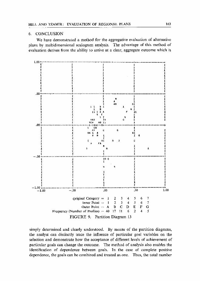
Example C The basic assumptions for this selection process are: a) all the conversion

functions between objectives and goals are linear apart from a convex relationship relating to goal variable 13. All the curves are monotonic; b) the objectives, pre- vention of industrial air pollution (by means of goal 13) and the removal of constraints on industrial production (by means of goal 1) are both more important than any of the other objectives. By analyzing the partition diagrams 1 (Figure 8) and 13 (Figure 9), we look for alternatives with the highest goal-achievement (1), the distance of which to alternative No. 3 is as small as possible. Alternative Nos. 5 and 7 meet these conditions:

Alternative5 ~ 1 4 1 1 4 2 1 1 4 5 4 --]--1 6 Alternative7 1 [ 1 5 1 1 2 2 1 1 3 1 5 1 I 5

The goal-achievement values for goal variables 1 and 13 are enclosed. On comparing their profile of values, alternative No. 7 emerges as the superior one. An examination of additional profiles (alternatives Nos. 15 and 44) in which there is a marginal reduction in the values of item 13 (from 1 to 2) or in which there is a marginal reduction in the value of item I (as in alternatives Nos. 25, 42, and 47) demon- strates their inferiority to alternative No. 7:


Al te rna t ive 15 1 1 4 1






1 2 1 1 2 1 2 3 2 8

1 1 2 1 1 2 5 5 2 9

1 1 3 1 2 2 3 4 1 5

1 2 4 4 3 5 2 5 1 8

1 2 3 2 2 3 1 4 1 6

1 2 2 1 1 3 1 5 1 5

1.00 + - - . . . . . . . . . . . . . . . . . + . . . . . . . . . . . . . . . . . . . * . . . . . . . . . . . . . . . . . . . . , . . . . . . . . . . . . . . . . . . . +

I I I I I I I [ I I I I I I I I I I I I I I I I I I I I I I I I I I I I I I I I I I I I I I I ! I I I I I I I

. 5 0 + . . . . . . . . . . . . . . . . . . ~ + . . . . . . . . . . . . . . . . . . . . + . . . . . . . . . . . . . . . . . . . + . . . . . . . . . . . . . . . . . . . +

[ I I I . I I I I 0 l I I I I C I I I I I CA CI I I I A O 8 I 3 . I I I I C D E I I I I 3A C A C. a IB I I I B n l I I I B I C I I I I OAA IA B I I I I COB CA I 0 I

,00'+ . . . . . . . . . . . . . . . . . . . + . . . . . . . . . . A-8C88--C§ . . . . . . . . . . . . . . . . . . . + . . . . . . . . . . . . . . . . . . . 5 I I 3 0 3 I I I ; 0 3 C I I I 3C 4 O 01 I I O C 1 1 E I I I I I 0 0 1 A B C I I r AA I I A I I I 0 B I I I I I I I I I

I I

. I I. I I

-.50 +.- . . . . . . . . . . . . . . . . . . * . . . . . . . . . . . . . . . . . . . + . . . . . . . . . . . . . . . . . . . + . . . . . . . . . . . . . . . . . . . + Z t o �9 z , I

I I I I I I I I I I I 3 3 I I I .I I I I I I X l I I I I I I I I I I

' I I I I I I I I I I I I I I I

-1.00 + ................... + ................... + ................... + ........ - .......... + - 1 . 0 0 - . 5 0 . 0 0 . 5 0 1 . 0 0

Original Category = 1 2 3 4 5 Inner Point = 1 2 3 4 5 Outer Point = A B C D E

Frequency (Number of Profiles) = 17 15 30 19 4

F I G U R E 8. Pa r t i t i on D i a g r a m 1

The o ther a l ternat ives fall away for the fo l lowing reasons : a) relat ive i m p o r t a n c e

of goals 1 a n d 13; b) the convexi ty of the convers ion func t i on re la t ing to goal 13;

c) the high aggregate goa l -ach ievement level o f a l te rna t ive No. 7.


6. CONCLUSION

We have demonstrated a method for the aggregative evaluation of alternative plans by multidimensional scalogram analysis. The advantage of this method of evaluation derives from the ability to arrive at a clear, aggregate outcome which is

1.00 + + + + + I I i I [ I I I I I I i I I I I I I I I I I I I I I I I I I I I I I I I I I I I I I I I I I I I I I I I I I I

. 5 0 ~" . . . . . . . . . . . . . . . . . . . + . . . . . . . . . . . . . . . . . . . * . . . . . . . . . . . . . . . . . . . . + . . . . . . . . . . . . . . . . . . . +

I [ I I I I I I B I I I t I A I I I I I AB GI I I I I i 8 I I I I I I t B A I I I I I t i a A g I t I I I A E X I I I t I A I I I I a02 IA G I I I I FJCA AO IG I

.00 + ................... +--- ....... t-t&iC--O~ ................... ~ ................... G I I i CA I I I VF C G I I I I IIS C A A I I I I A B I I A I I I I I I [ G At P 0 C I I [ ~ FA ! I I 8 I r I I 3 B I A I I I I I I I I I I I

--.~0 ~ ........................ + " .................................. + + " ...... ~ ......... + I ,I ID C I I I ~ z z ! I I I I

r I I I I I I I I I I I I I

I I I I I I I I I I I ! I l I I I I I I

- - 1.00 --.50 .00 .50 1.00

original Category = 1 2 3 4 5 6 7 Inner Point = 1 2 3 4 5 6 7 Outer Point = A B C D E F G

Frequency (Number of Profiles) = 40 17 11 6 2 4 5

F I G U R E 9. Part i t ion D i a g r a m 13

simply determined and clearly understood. By means of the partition diagrams, the analyst can distinctly trace the influence of particular goal variables on the selection and demonstrate how the acceptance of different levels of achievement of particular goals can change the outcome. The method of analysis also enables the identification of dependence between goals. In the case of complete positive dependence, the goals can be combined and treated as one. Thus, the total number


of goals is reduced, facilitating greater comprehension of the effects of the individual goals and simplifying the analysis. Conflict between objectives is expressed in the analysis by negative dependence.

Differential weights of goals can also be incorporated. If these are introduced a priori, a different configuration of plans in the space diagram is likely to emerge. Alternatively, the effect of differential weighting of goals on the outcome can be determined (as in examples B and C) by analyzing the configuration of plans ini- tially based on assumed equal goal weights in conjunction with the relevant partition diagrams (of the individual goals). The method of evaluation is not restricted to an assumed linear valuation of marginal goal achievement. The increments of goal-achievement of particular goals can be differentially weighted either on an a priori basis or by analyzing the profiles of goal achievement with respect to the aggregate outcomes expressed in the space diagram. The example employed for testing the efficacy of M.S.A. was solely based on physical goals for reasons of convenience. This, however, is not inherent in the analysis. Economic and social goals, at whatever level in the goal hierarchy under consideration, can similarily be incorporated, provided that they can be measured on an ordinal scale, at least. While M.S.A. translates the outcomes into ordinal scales, this is not finally binding, and goal-achievement levels can easily be translated back into higher level (interval or ratio) scales in order to establish trade-off relationships (as in Example B). The resolution of conflict between objectives, with respect to the particular planning problem under consideration, can be incorporated in two ways: a) by weighting objectives--the value of an objective with respect to others with which it is in conflict is explicitly stated; b) among the alternative plans available, that plan can be identified which, more than any other, reduces the level of conflict among objectives.

The method, as demonstrated, is probably most useful for evaluating a large number of alternative plans intended to achieve a relatively large number of goals. The demonstrated application is but a first experiment and the full potential of the method awaits further investigation. In summary, the proposed method of selection facilitates rational decision on the basis of the consideration of all the components and interrelationships of the plans, thereby overcoming many of the disadvantages cited with respect to other aggregative methods of plan evaluation. The analysts and decision-makers do not abdicate their role in the selection process to a mechanistic aggregative formula which involves implicit assumptions. Nevertheless, they can play a significant role in the process whereby the logic of decision is constantly tested and value preferences can be explicitly and clearly incorporated.

REFERENCES

[1] Ackoff, R. Scientific Method: Optimizing Applied Research Decisions. Wiley, 1962.

[2] Boyce, D., N. D. Day, and C. McDonald. Metropolitan Plan Making. No. 4. Philadelphia: Regional Science Research Institute, 1970.

New York: John

Monograph Series


[311 Dash, Y. and E. Efrat. Israel Physical Master Plan. Jerusalem: Ministry of Interior, 1967.

[411 Fishburn, P. Decision and Value Theory. New York: John Wiley, 1964. [511 Freeman, A.M. "Project Decision and Evaluation with Multiple Objectives," in R.H.

Haveman and J. Margolis (Eds.), Public Expenditures and Policy Analysis. Chicago: Markham, 1970.

[611 Hill, M. "A Goals-Achievement Matrix for Evaluating Alternative Plans," Journal of the American Institute of Planners, Vol. 36 (January 1968), pp. 19-29.

[7] Planning for Multiple Objectives. Monograph Series No. 5. Philadelphia: Regional Science Research Institute, 1973.

[8] - - and M. Shechter. "Optimal Goal Achievement in the Development of Outdoor Recreation Facilities," in A.G. Wilson (Ed.), Urban and Regional Planning. London: Pion Press, 1971.

[9] Krutilla, J.V. "Welfare Aspects of Benefit-Cost Analysis," Journal of Political Economy, Vol. 69 (June 1961), pp. 226-255.

[10] Leven, C. "Establishing Goals for Regional Development," Journal of the American Institute o f Planners, Vol. 30 (May 1964), pp. 100-110.

[ll!f Lichfield, N. "'Cost-Benefit Analysis in City Planning," Journal o f the American lnstitute o f Planners, Vol. 26 (November 1960), pp. 273-279.

[12] "Cost-Benefit Analysis in Plan Evaluation," Town Planning Review, Vol. 35 (July 1964), pp. 160-164.

[13] Lingoes, J.C. "An IBM-7090 Program for Guttman-Lingoes Multidimensional Scalogram Analysis--I," Behavioral Science, Vol. 11 (January 1966), pp. 76-78.

[14] "The Multivariate Analysis of Qualitative Data," Multivariate Behavioral Research, Vol. 13 (January 1968), pp. 61-94.

[15] Manheim, M. and F. Hall. "Abstract Representation of Goals: A Method for Making Decisions on Complex Problems," Manuscript, Department of Civil Engineering, Massa- chusetts Institute of Technology, Cambridge, Mass., 1968.

[16] McGuire, M. C. and H. A. Garn. "Integration of Equity and Efficiency Criteria," Economic Journal, Vol. 79 (December 1969), pp. 882-893.

[17] Reiner, T.A. "A Multiple Goals Framework for Regional Planning," Papers of the Regional Science Association, Vol. 26 (1971), pp. 206-239.

[18] Steiner, P.O. "The Public Sector and the Public Interest," in R. H. Haveman and J. Mar- golis (Eds.), Public Expenditure and Policy Analysis. Chicago: Markham, t970.

[19.1 Tzamir, Y. "Aggregative EValuation of Alternative Physical Plans by Multidimensional Analysis," Unpublished thesis for the degree of Master of Architecture and Town Planning, Technion-Israel Institute of Technology, Haifa, 1970.

multidimensional evaluation of regional plans serving multiple objectives

Documents