Multi-view Laplacian Support Vector Machines

Shiliang Sun

Department of Computer Science and Technology,East China Normal University, Shanghai 200241, China

slsun@cs.ecnu.edu.cn

Abstract. We propose a new approach, multi-view Laplacian supportvector machines (SVMs), for semi-supervised learning under the multi-view scenario. It integrates manifold regularization and multi-view regu-larization into the usual formulation of SVMs and is a natural extensionof SVMs from supervised learning to multi-view semi-supervised learn-ing. The function optimization problem in a reproducing kernel Hilbertspace is converted to an optimization in a finite-dimensional Euclideanspace. After providing a theoretical bound for the generalization per-formance of the proposed method, we further give a formulation of theempirical Rademacher complexity which affects the bound significantly.From this bound and the empirical Rademacher complexity, we can gaininsights into the roles played by different regularization terms to thegeneralization performance. Experimental results on synthetic and real-world data sets are presented, which validate the effectiveness of theproposed multi-view Laplacian SVMs approach.

Key words: graph Laplacian, multi-view learning, reproducing kernelHilbert space, semi-supervised learning, support vector machine

1 Introduction

Semi-supervised learning or learning from labeled and unlabeled examples hasattracted considerable attention in the last decade [1–3]. This is partially moti-vated by the fact that for many practical applications collecting a large numberof unlabeled data is much less involved than collecting labeled data consideringthe expensive and tedious annotation process. Moreover, as human learning oftenoccurs in the semi-supervised learning manner (for example, children may hearsome words but do not know their exact meanings), research on semi-supervisedlearning also has the potential to uncover insights into mechanisms of humanlearning [4].

In some machine learning applications, examples can be described by differ-ent kinds of information. For example, in television broadcast understanding,broadcast segments can be simultaneously described by their video signals andaudio signals which can be regarded as information from different properties ordifferent “views”. Multi-view semi-supervised learning, the focus of this paper,attempts to perform inductive learning under such circumstances. However, it

should be noted that if there are no natural multiple views, artificially generatedmultiple views can still work favorably [5].

In this paper we are particularly interested in multi-view semi-supervisedlearning approaches derived from support vector machines (SVMs) [6]. As astate-of-the-art method in machine learning, SVMs not only are theoretically welljustified but also show very good performance for real applications. The trans-ductive SVMs [7], S3VMs [8, 9] and Laplacian SVMs [10] have been proposedas extensions of SVMs from supervised learning to single-view semi-supervisedlearning. For multi-view learning, there are also several extensions of SVMs pro-posed such as the co-Laplacian SVMs [11] and SVM-2K [12].

Regularization theory is an important technique in mathematics and machinelearning [13, 14]. Many methods can be explained from the point of view ofregularization. A close parallel to regularization theory is capacity control offunction classes [15]. Both regularization and capacity control of function classescan play a central role in alleviating over-fitting of machine learning algorithms.

The new method, multi-view Laplacian SVMs, proposed in this paper canalso be explained by regularization theory and capacity control of functionclasses. It integrates three regularization terms respectively on function norm,manifold and multi-view regularization. As an appropriate integration of themand thus the effective use of information from labeled and unlabeled data, ourmethod has the potential to outperform many related counterparts. The differ-ent roles of these regularization terms on capacity control will be unfolded lateras a result of our empirical Rademacher complexity analysis. Besides giving thebound on the generalization error, we also report experimental results of theproposed method on synthetic and real-world data sets.

The layout of this paper is as follows. Section 2 introduces the objective func-tion of the proposed approach with concerns on different regularization terms,and its optimization. Theoretical insights on the generalization error and theempirical Rademacher complexity are covered by Section 3. Then, experimentalresults are reported in Section 4. Finally, conclusions are drawn in Section 5.

2 Multi-view Laplacian SVMs (MvLapSVM)

2.1 Manifold Regularization

Let x1, . . . , xl+u ∈ Rd denote a set of inputs including l labeled examples andu unlabeled ones with label space {+1,−1}. For manifold regularization, a dataadjacency graph W(l+u)×(l+u) is defined whose entries measure the similarity orcloseness of every pair of inputs. We use a typical construction of W : Wij = 0for most pairs of inputs, and for neighboring xi, xj the corresponding entry isgiven by

Wij = exp(−‖xi − xj‖2/2σ2), (1)

where ‖xi − xj‖ is the Euclidean norm in Rd.

The manifold regularization functional acting on any function f : Rd → Ris defined as follows [16]

Mreg(f) =1

2

l+u∑

i,j=1

Wij(f(xi) − f(xj))2. (2)

It is clear that a smaller Mreg(f) indicates a smoother function f . Define vectorf = (f(x1), . . . , f(xl+u))>. Then

Mreg(f) =

l+u∑

i=1

(

l+u∑

j=1

Wij)f2(xi) −

l+u∑

i,j=1

Wijf(xi)f(xj)

= f>(V − W )f, (3)

where matrix V is diagonal with the ith diagonal entry Vii =∑l+u

j=1 Wij . The

matrix L , V − W , which is arguably positive semidefinite, is called the graphLaplacian of W . In our empirical studies in Section 4, a normalized LaplacianL = V −1/2LV −1/2 is used because this normalized one often performs as well orbetter in practical tasks [10].

2.2 Multi-view Regularization

For multi-view learning, an input x ∈ Rd can be decomposed into componentscorresponding to multiple views, such as x = (x1, . . . , xm) for an m-view repre-sentation. A function fj defined on view j only depends on xj , while ignoringthe other components (x1, . . . , xj−1, xj+1, . . . , xm).

For multi-view semi-supervised learning, there is a commonly acceptable as-sumption that a good learner can be learned from each view [17]. Consequently,these good learners in different views should be consistent to a large extentwith respect to their predictions on the same examples. We also adopt this as-sumption and use the regularization idea to wipe off those inconsistent learners.Given the l+u examples, the multi-view regularization functional for m functionsf1, . . . , fm can be formulated as

Vreg(f1, . . . , fm) =m

∑

j>k,k=1

l+u∑

i=1

[fj(xi) − fk(xi)]2. (4)

Clearly, a smaller Vreg(f1, . . . , fm) tends to find good learners in each view.

2.3 MvLapSVM

As is usually assumed in multi-view learning, each view is regarded to be suf-ficient to train a good learner. Therefore, we can write the final prediction asf = 1

m

∑mi=1 fi. For MvLapSVM, in this paper we concentrate on the two-view

case, that is m = 2. In this scenario, the objective function for MvLapSVM isdefined as

minf1∈H1,f2∈H2

1

2l

l∑

i=1

[(1 − yif1(xi))+ + (1 − yif2(xi))+] +

γ1(‖f1‖2 + ‖f2‖

2) +γ2

(l + u)2(f1

>L1f1 +

f2>L2f2) +

γ3

(l + u)

l+u∑

i=1

[f1(xi) − f2(xi)]2, (5)

where H1,H2 are the reproducing kernel Hilbert spaces [18, 19] in which f1, f2

are defined, nonnegative scalars γ1, γ2, γ3 are respectively norm regularization,manifold regularization and multi-view regularization coefficients, and vectorf1 = (f1(x1), ..., f1(xl+u))>, f2 = (f2(x1), ..., f2(xl+u))>.

2.4 Optimization

We now concentrate on solving (5). As an application of the representer theo-rem [20, 21], the solution to problem (5) has the following form

f1(x) =l+u∑

i=1

αi1k1(xi, x), f2(x) =

l+u∑

i=1

αi2k2(xi, x). (6)

Therefore, we can rewrite ‖f1‖2 and ‖f2‖

2 as

‖f1‖2 = α

>1 K1α1, ‖f2‖

2 = α>2 K2α2, (7)

where K1 and K2 are (l + u) × (l + u) Gram matrices respective from view V1

and V2, and vector α1 = (α11, ..., α

l+u1 )>, α2 = (α1

2, ..., αl+u2 )>. In addition, we

have

f1 = K1α1, f2 = K2α2. (8)

To simplify our formulations, we respectively replaceγ2

(l + u)2and

γ3

(l + u)in

(5) with γ2 and γ3. Thus, the primal problem can be reformulated as

minα1,α2,ξ1,ξ2

F0 =1

2l

l∑

i=1

(ξi1 + ξi

2) + γ1(α>1 K1α1 +

α>2 K2α2) + γ2(α

>1 K1L1K1α1 + α

>2 K2L2K2α2) +

γ3(K1α1 − K2α2)>(K1α1 − K2α2)

s.t.

yi(∑l+u

j=1 αj1k1(xj , xi)) ≥ 1 − ξi

1,

yi(∑l+u

j=1 αj2k2(xj , xi)) ≥ 1 − ξi

2,

ξi1, ξi

2 ≥ 0, i = 1, . . . , l ,

(9)

where yi ∈ {+1,−1}, γ1, γ2, γ3 ≥ 0. Note that the additional bias terms areembedded in the weight vectors of the classifiers by using the example represen-tation of augmented vectors.

We present two theorems concerning the convexity and strong duality (whichmeans the optimal value of a primal problem is equal to that of its Lagrangedual problem [22]) of problem (9) with proofs omitted.

Theorem 1. Problem (9) is a convex optimization problem.

Theorem 2. Strong duality holds for problem (9).

Suppose λi1, λ

i2 ≥ 0 are the Lagrange multipliers associated with the first two

sets of inequality constraints of problem (9). Define λ1 = (λ11, ..., λ

l1)

> and λ2 =(λ1

2, ..., λl2)

>. It can be shown that the Lagrangian dual optimization problemwith respect to λ1 and λ2 is a quadratic program. Classifier parameters α1 andα2 used by (6) can be solved readily after we get λ1 and λ2.

3 Theoretical Analysis

In this section, we give a theoretical analysis of the generalization error of theMvLapSVM method in terms of the theory of Rademacher complexity bounds.

3.1 Background Theory

Some important background on Rademacher complexity theory is introduced asfollows.

Definition 1 (Rademacher complexity, [15, 23, 24]). For a sample S ={x1, . . . , xl} generated by a distribution Dx on a set X and a real-valued functionclass F with domain X, the empirical Rademacher complexity of F is the randomvariable

Rl(F) = Eσ[supf∈F

|2

l

l∑

i=1

σif(xi)||x1, . . . , xl],

where σ = {σ1, . . . , σl} are independent uniform {±1}-valued (Rademacher)random variables. The Rademacher complexity of F is

Rl(F) = ES [Rl(F)] = ESσ[supf∈F

|2

l

l∑

i=1

σif(xi)|].

Lemma 1 ([15]). Fix δ ∈ (0, 1) and let F be a class of functions mappingfrom an input space Z (for supervised learning having the form Z = X × Y ) to[0, 1]. Let (zi)

li=1 be drawn independently according to a probability distribution

D. Then with probability at least 1 − δ over random draws of samples of size l,every f ∈ F satisfies

ED[f(z)] ≤ E[f(z)] + Rl(F) +

√

ln(2/δ)

2l

≤ E[f(z)] + Rl(F) + 3

√

ln(2/δ)

2l,

where E[f(z)] is the empirical error averaged on the l examples.

Note that the above lemma is also applicable if we replace [0, 1] by [−1, 0].This can be justified by simply following the proof of Lemma 1, as detailedin [15].

3.2 The Generalization Error of MvLapSVM

We obtain the following theorem regarding the generalization error of MvLapSVM,which is similar to one theorem in [12]. The prediction function in MvLapSVMis adopted as the average of prediction functions from two views

g =1

2(f1 + f2). (10)

Theorem 3. Fix δ ∈ (0, 1) and let F be the class of functions mapping fromZ = X×Y to R given by f(x, y) = −yg(x) where g = 1

2 (f1+f2) ∈ G and f ∈ F .Let S = {(x1, y1), · · · , (xl, yl)} be drawn independently according to a probabilitydistribution D. Then with probability at least 1 − δ over samples of size l, everyg ∈ G satisfies

PD(y 6= sgn(g(x))) ≤1

2l

l∑

i=1

(ξi1 + ξi

2) + 2Rl(G) + 3

√

ln(2/δ)

2l,

where ξi1 = (1 − yif1(xi))+ and ξi

2 = (1 − yif2(xi))+.

Proof. Let H(·) be the Heaviside function that returns 1 if its argument is greaterthan 0 and zero otherwise. Then it is clear to have

PD(y 6= sgn(g(x))) = ED[H(−yg(x))]. (11)

Consider a loss function A : R → [0, 1], given by

A(a) =

1, if a ≥ 0;1 + a, if −1 ≤ a ≤ 0;0, otherwise.

By Lemma 1 and since function A− 1 dominates H − 1, we have [15]

ED[H(f(x, y)) − 1] ≤ ED[A(f(x, y)) − 1]

≤ E[A(f(x, y)) − 1] + Rl((A− 1) ◦ F) + 3

√

ln(2/δ)

2l.

Therefore,

ED[H(f(x, y))]

≤ E[A(f(x, y))] + Rl((A− 1) ◦ F) + 3

√

ln(2/δ)

2l. (12)

In addition, we have

E[A(f(x, y))] ≤1

l

l∑

i=1

(1 − yig(xi))+

=1

2l

l∑

i=1

(1 − yif1(xi) + 1 − yif2(xi))+

≤1

2l

l∑

i=1

[(1 − yif1(xi))+ + (1 − yif2(xi))+]

=1

2l

l∑

i=1

(ξi1 + ξi

2), (13)

where ξi1 denotes the amount by which function f1 fails to achieve margin 1 for

(xi, yi) and ξi2 applies similarly to function f2.

Since (A − 1)(0) = 0, we can apply the Lipschitz condition [23] of function(A− 1) to get

Rl((A− 1) ◦ F) ≤ 2Rl(F). (14)

It remains to bound the empirical Rademacher complexity of the class F . Withyi ∈ {+1,−1}, we have

Rl(F) = Eσ[supf∈F

|2

l

l∑

i=1

σif(xi, yi)|]

= Eσ[supg∈G

|2

l

l∑

i=1

σiyig(xi)|]

= Eσ[supg∈G

|2

l

l∑

i=1

σig(xi)|] = Rl(G). (15)

Now combining (11)∼(15) reaches the conclusion of this theorem. ut

3.3 The Empirical Rademacher Complexity Rl(G)

In this section, we give the expression of Rl(G) used in Theorem 3. Rl(G) isalso important in identifying the different roles of regularization terms in theMvLapSVM approach. The techniques adopted to derive Rl(G) is analogical toand inspired by those used for analyzing co-RLS in [19, 24].

The loss function L : H1 × H2 → [0,∞) in (5) with L = 12l

∑li=1[(1 −

yif1(xi))+ + (1 − yif2(xi))+] satisfies

L(0, 0) = 1. (16)

We now derive the regularized function class G from which our predictor g isdrawn.

Let Q(f1, f2) denote the objective function in (5). Substituting the predictorsf1 ≡ 0 and f2 ≡ 0 into Q(f1, f2) results in an upper bound

minf1,f2∈H1×H2

Q(f1, f2) ≤ Q(0, 0) = L(0, 0) = 1. (17)

Because each term in Q(f1, f2) is nonnegative, the optimal function pair (f∗1 , f∗

2 )minimizing Q(f1, f2) must be contained in

H = {(f1, f2) : γ1(‖f1‖2 + ‖f2‖

2) + γ2(f1u>L1uf1u +

f2u>L2uf2u) + γ3

l+u∑

i=l+1

[f1(xi) − f2(xi)]2 ≤ 1}, (18)

where parameters γ1, γ2, γ3 are from (9), f1u = (f1(xl+1), ..., f1(xl+u))>, f2u =(f2(xl+1), ..., f2(xl+u))>, and L1u and L2u are the unnormalized graph Lapla-cians for the graphs only involving the unlabeled examples (to make theoreticalanalysis on Rl(G) feasible, we temporarily assume that the Laplacians in (5) areunnormalized).

The final predictor is found out from the function class

G = {x →1

2[f1(x) + f2(x)] : (f1, f2) ∈ H}, (19)

which does not depend on the labeled examples.The complexity Rl(G) is

Rl(G) = Eσ[ sup(f1,f2)∈H

|1

l

l∑

i=1

σi(f1(xi) + f2(xi))|]. (20)

To derive the Rademacher complexity, we first convert from a supremum overthe functions to a supremum over their corresponding expansion coefficients.Then, the Kahane-Khintchine inequality [25] is employed to bound the expec-tation over σ above and below, and give a computable quantity. The followingtheorem summarizes our derived Rademacher complexity.

Theorem 4. Suppose S = K1l(γ1K1 + γ2K>1uL1uK1u)−1K>

1l + K2l(γ1K2 +γ2K

>2uL2uK2u)−1K>

2l , Θ = K1u(γ1K1 + γ2K>1uL1uK1u)−1K>

1u + K2u(γ1K2 +γ2K

>2uL2uK2u)−1K>

2u, J = K1u(γ1K1 + γ2K>1uL1uK1u)−1K>

1l − K2u(γ1K2 +γ2K

>2uL2uK2u)−1K>

2l , where K1l and K2l are respectively the first l rows of K1

and K2, and K1u and K2u are respectively the last u rows of K1 and K2. Thenwe have U√

2l≤ Rl(G) ≤ U

l with U2 = tr(S) − γ3tr(J>(I + γ3Θ)−1J ).

4 Experiments

We performed multi-view semi-supervised learning experiments on a syntheticand two real-world classification problems. The Laplacian SVM (LapSVM) [10],co-Laplacian SVM (CoLapSVM) [11], manifold co-regularization (CoMR) [19]and co-SVM (a counterpart of the co-RLS in [11]) are employed for comparisonswith our proposed method. For each method, besides considering the predictionfunction (f1 + f2)/2 for the combined view, we also consider the predictionfunctions f1 and f2 from the separate views.

Each data set is divided into a training set (including labeled and unlabeledtraining data), a validation set and a test set. The validation set is used to selectregularization parameters from the range {10−10, 10−6, 10−4, 10−2, 1, 10, 100},and choose which prediction function should be used. With the identified regu-larization parameter and prediction function, performances on the test data andunlabeled training data would be evaluated. The above process is repeated atrandom for ten times, and the reported performance is the averaged accuracyand the corresponding standard deviation.

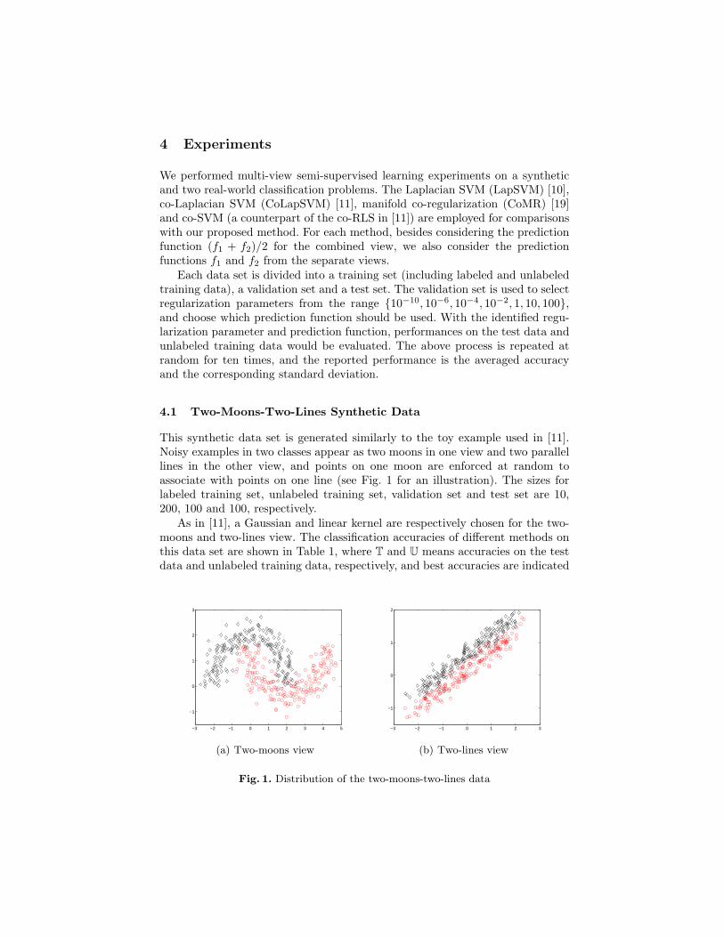
4.1 Two-Moons-Two-Lines Synthetic Data

This synthetic data set is generated similarly to the toy example used in [11].Noisy examples in two classes appear as two moons in one view and two parallellines in the other view, and points on one moon are enforced at random toassociate with points on one line (see Fig. 1 for an illustration). The sizes forlabeled training set, unlabeled training set, validation set and test set are 10,200, 100 and 100, respectively.

As in [11], a Gaussian and linear kernel are respectively chosen for the two-moons and two-lines view. The classification accuracies of different methods onthis data set are shown in Table 1, where T and U means accuracies on the testdata and unlabeled training data, respectively, and best accuracies are indicated

−3 −2 −1 0 1 2 3 4 5

−1

0

1

2

3

(a) Two-moons view

−3 −2 −1 0 1 2 3

−1

0

1

2

(b) Two-lines view

Fig. 1. Distribution of the two-moons-two-lines data

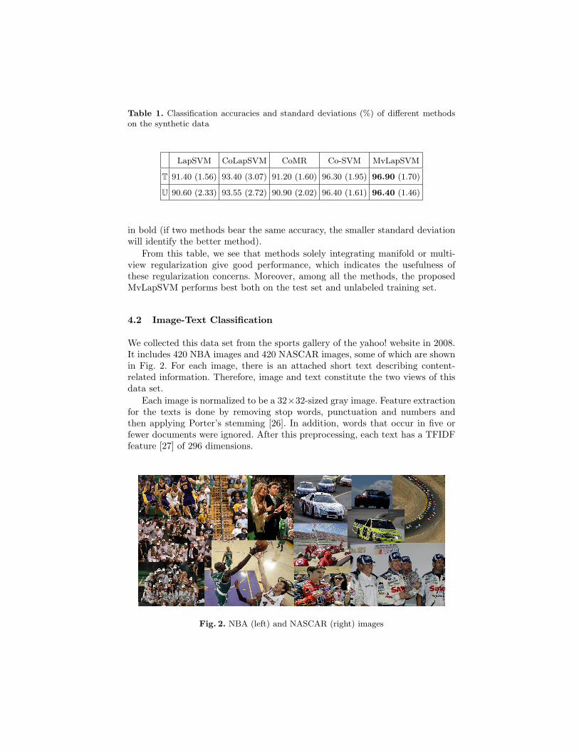
Table 1. Classification accuracies and standard deviations (%) of different methodson the synthetic data

LapSVM CoLapSVM CoMR Co-SVM MvLapSVM

T 91.40 (1.56) 93.40 (3.07) 91.20 (1.60) 96.30 (1.95) 96.90 (1.70)

U 90.60 (2.33) 93.55 (2.72) 90.90 (2.02) 96.40 (1.61) 96.40 (1.46)

in bold (if two methods bear the same accuracy, the smaller standard deviationwill identify the better method).

From this table, we see that methods solely integrating manifold or multi-view regularization give good performance, which indicates the usefulness ofthese regularization concerns. Moreover, among all the methods, the proposedMvLapSVM performs best both on the test set and unlabeled training set.

4.2 Image-Text Classification

We collected this data set from the sports gallery of the yahoo! website in 2008.It includes 420 NBA images and 420 NASCAR images, some of which are shownin Fig. 2. For each image, there is an attached short text describing content-related information. Therefore, image and text constitute the two views of thisdata set.

Each image is normalized to be a 32×32-sized gray image. Feature extractionfor the texts is done by removing stop words, punctuation and numbers andthen applying Porter’s stemming [26]. In addition, words that occur in five orfewer documents were ignored. After this preprocessing, each text has a TFIDFfeature [27] of 296 dimensions.

Fig. 2. NBA (left) and NASCAR (right) images

Table 2. Classification accuracies and standard deviations (%) of different methodson the NBA-NASCAR data

LapSVM CoLapSVM CoMR Co-SVM MvLapSVM

T 99.33 (0.68) 98.86 (1.32) 99.38 (0.68) 99.43 (0.59) 99.38 (0.64)

U 99.03 (0.88) 98.55 (0.67) 98.99 (0.90) 98.91 (0.38) 99.54 (0.56)

The sizes for labeled training set, unlabeled training set, validation set andtest set are 10, 414, 206 and 210, respectively. Linear kernels are used for bothviews. The performance is reported in Table 2 where co-SVM ranks first on thetest set while MvLapSVM outperforms all the other methods on the unlabeledtraining set. If we take the average of the accuracies on the test set and unlabeledtraining set, clearly our MvLapSVM ranks first.

4.3 Web Page Categorization

In this subsection, we consider the problem of classifying web pages. The dataset consists of 1051 two-view web pages collected from the computer science de-partment web sites at four U.S. universities: Cornell, University of Washington,University of Wisconsin, and University of Texas [17]. The task is to predictwhether a web page is a course home page or not. Within the data set there area total of 230 course home pages. The first view of the data is the words ap-pearing on the web page itself, whereas the second view is the underlined wordsin all links pointing to the web page from other pages. We preprocess each viewaccording to the feature extraction procedure used in Section 4.2. This results in2332 and 87-dimensional vectors in view 1 and view 2 respectively [28]. Finally,document vectors were normalized to TFIDF features.

Table 3. Classification accuracies and standard deviations (%) of different methodson the web page data

LapSVM CoLapSVM CoMR Co-SVM MvLapSVM

T 94.02 (2.66) 93.68 (2.98) 94.02 (2.24) 93.45 (3.21) 94.25 (1.62)

U 93.33 (2.40) 93.39 (2.44) 93.26 (2.19) 93.16 (2.68) 93.53 (2.04)

The sizes for labeled training set, unlabeled training set, validation set andtest set are 12, 519, 259 and 261, respectively. Linear kernels are used for bothviews. Table 3 gives the classification results obtained by different methods.MvLapSVM outperforms all the other methods on both the test data and unla-beled training data.

5 Conclusion

In this paper, we have proposed a new approach for multi-view semi-supervisedlearning. This approach is an extension of SVMs for multi-view semi-supervisedlearning with manifold and multi-view regularization integrated. We have provedthe convexity and strong duality of the primal optimization problem, and usedthe dual optimization to solve classifier parameters. Moreover, theoretical resultson the generalization performance of the MvLapSVM approach and the empiricalRademacher complexity which can indicate different roles of regularization termshave been made. Experimental practice on multiple data sets has also manifestedthe effectiveness of the proposed method.

The MvLapSVM is not a special case of the framework that Rosenberg et al.formulated in [29]. The main difference is that they require the loss functionaldepends only on the combined prediction function, while we use here a slightlygeneral loss which has a separate dependence on the prediction function fromeach view. Their framework does not subsume our approach.

For future work, we mention the following three directions.

– Model selection: As is common in many machine learning algorithms, ourmethod has several regularization parameters to set. Usually, a held outvalidation set would be used to perform parameter selection, as what wasdone in this paper. However, for the currently considered semi-supervisedlearning, this is not very natural because there is often a small quantityof labeled examples available. Model selection for semi-supervised learningusing no or few labeled examples is worth further studying.

– Multi-class classification: The MvLapSVM algorithm implemented inthis paper is intended for binary classification. Though the usual one-versus-rest, one-versus-another strategy, which converts a problem from multi-classto binary classification, can be adopted for multi-class classification, it isnot optimal. Incorporating existing ideas of multi-class SVMs [30] into theMvLapSVM approach would be a further concern.

– Regularization selection: In this paper, although the MvLapSVM al-gorithm obtained good results, it involves more regularization terms thanrelated methods and thus needs more assumptions. For some applications,these assumptions might not hold. Therefore, a probably interesting improve-ment could be comparing different kinds of regularizations and attempting toselect those promising ones for each application. This also makes it possibleto weight different views unequally.

Acknowledgments. This work was supported in part by the National NaturalScience Foundation of China under Project 61075005, and the FundamentalResearch Funds for the Central Universities.

References

1. Chapelle, O., Scholkopf, B., Zien, A.: Semi-supervised Learning. MIT Press, Cam-bridge, MA (2006)

2. Culp, M., Michailidis, G.: Graph-based Semi-supervised Learning. IEEE Transac-tions on Pattern Analysis and Machine Intelligence, Vol. 30 (2008) 174–179

3. Sun, S., Shawe-Taylor, J.: Sparse Semi-supervised Learning using Conjugate Func-tions. Journal of Machine Learning Research, Vol. 11 (2010) 2423–2455

4. Zhu, X.: Semi-supervised Learning Literature Survey. Technical Report, 1530, Uni-versity of Wisconsin-Madison (2008)

5. Sun, S., Jin, F., Tu, W.: View Construction for Multi-view Semi-supervised Learn-ing. Lecture Notes in Computer Science, Vol. 6675 (2011) 595–601

6. Vapnik, V.N.: Statistical Learning Theory. Wiley, New York (1998)7. Joachims, T.: Transductive Inference for Text Classification using Support Vector

Machines. Proceedings of the 16th International Conference on Machine Learning(1999) 200–209

8. Bennett, K., Demiriz, A.: Semi-supervised Support Vector Machines. Advances inNeural Information Processing Systems, Vol. 11 (1999) 368–374

9. Fung, G., Mangasarian, O.L.: Semi-supervised Support Vector Machines for Un-labeled Data Classification. Optimization Methods and Software, Vol. 15 (2001)29–44

10. Belkin, M., Niyogi, P., Sindhwani, V.: Manifold Regularization: A GeometricFramework for Learning from Labeled and Unlabeled Exampls. Journal of Ma-chine Learning Research, Vol. 7 (2006) 2399–2434

11. Sindhwani, V., Niyogi, P., Belkin, M.: A Co-regularization Approach to Semi-supervised Learning with Multiple Views. Proceedings of the Workshop on Learn-ing with Multiple Views, International Conference on Machine Learning (2005)

12. Farquhar, J., Hardoon, D., Meng, H., Shawe-Taylor, J., Szedmak, S.: Two ViewLearning: SVM-2K, Theory and Practice. Advances in Neural Information Pro-cessing Systems, Vol. 18 (2006) 355–362

13. Tikhonov, A.N.: Regularization of Incorrectly Posed Problems. Soviet MathematicsDoklady, Vol. 4 (1963) 1624–1627

14. Evgeniou, T., Pontil, M., Poggio, T.: Regularization Networks and Support VectorMachines. Advances in Computational Mathematics, Vol. 13 (2000) 1–50

15. Shawe-Taylor, J., Cristianini, N.: Kernel Methods for Pattern Analysis. CambridgeUniversity Press, Cambridge, England (2004)

16. Belkin, M., Niyogi, P.: Laplacian Eigenmaps for Dimensionality Reduction andData Representation. Neural Computation, Vol. 15 (2003) 1373–1396

17. Blum, A., Mitchell, T.: Combining Labeled and Unlabeled Data with Co-training.Proceedings of the 11th Annual Conference on Computational Learning Theory(1998) 92–100

18. Aronszajn, N.: Theory of Reproducing Kernels. Transactions of the AmericanMathematical Society, Vol. 68 (1950) 337–404

19. Sindhwani, V., Rosenberg, D.: An RKHS for Multi-view Learning and ManifoldCo-regularization. Proceedings of the 25th International Conference on MachineLearning (2008) 976–983

20. Kimeldorf, G., Wahba, G.: Some Results on Tchebycheffian Spline Functions. Jour-nal of Mathematical Analysis and Applications, Vol. 33 (1971) 82–95

21. Rosenberg, D.: Semi-Supervised Learning with Multiple Views. PhD dissertation,Department of Statistics, University of California, Berkeley (2008)

22. Boyd, S., Vandenberghe, L.: Convex Optimization. Cambridge University Press,Cambridge, England (2004)

23. Bartlett, P., Mendelson, S.: Rademacher and Gaussian Complexities: Risk Boundsand Structural Results. Journal of Machine Learning Research, Vol. 3 (2002) 463–482

24. Rosenberg, D., Bartlett, P.: The Rademacher Complexity of Co-regularized KernelClasses. Proceedings of the 11th International Conference on Artificial Intelligenceand Statistics (2007) 396–403

25. Latala, R., Oleszkiewicz, K.: On the Best Constant in the Khintchine-KahaneInequality. Studia Mathematica, Vol. 109 (1994) 101–104

26. Porter, M.F.: An Algorithm for Suffix Stripping. Program, Vol. 14 (1980) 130–13727. Salton, G., Buckley, C.: Term-Weighting Approaches in Automatic Text Retrieval.

Information Processing and Management, Vol. 24 (1988) 513–52328. Sun, S.: Semantic Features for Multi-view Semi-supervised and Active Learning

of Text Classification. Proceedings of the IEEE International Conference on DataMining Workshops (2008) 731–735

29. Rosenberg, D., Sindhwani, V., Bartlett, P., Niyogi, P.: Multiview Point CloudKernels for Semisupervised Learning. IEEE Signal Processing Magazine (2009)145–150

30. Hsu, C.W., Lin, C.J.: A Comparison of Methods for Multiclass Support VectorMachines. IEEE Transactions on Neural Networks, Vol. 13 (2002) 415–425