multi-temporal land cover classification with long … · key words: long short-term memory,...

MULTI-TEMPORAL LAND COVER CLASSIFICATION WITH LONG SHORT-TERMMEMORY NEURAL NETWORKS

M. Rußwurm∗, M. Korner

Technical University of Munich, Chair of Remote Sensing Technology, Computer Vision Research GroupArcisstraße 21, 80333 Munich, Germany – {marc.russwurm,marco.koerner}@tum.de

Commission III, WG III/7

KEY WORDS: Long Short-Term Memory, Recurrent Neural Networks, Sentinel 2, Crop Identification, Deep Learning, Land CoverClassification

ABSTRACT:

Land cover classification (LCC) is a central and wide field of research in earth observation and has already put forth a variety ofclassification techniques. Many approaches are based on classification techniques considering observation at certain points in time.However, some land cover classes, such as crops, change their spectral characteristics due to environmental influences and can thusnot be monitored effectively with classical mono-temporal approaches. Nevertheless, these temporal observations should be utilized tobenefit the classification process. After extensive research has been conducted on modeling temporal dynamics by spectro-temporalprofiles using vegetation indices, we propose a deep learning approach to utilize these temporal characteristics for classification tasks.In this work, we show how long short-term memory (LSTM) neural networks can be employed for crop identification purposeswith SENTINEL 2A observations from large study areas and label information provided by local authorities. We compare thesetemporal neural network models, i.e., LSTM and recurrent neural network (RNN), with a classical non-temporal convolutional neuralnetwork (CNN) model and an additional support vector machine (SVM) baseline. With our rather straightforward LSTM variant, weexceeded state-of-the-art classification performance, thus opening promising potential for further research.

1. INTRODUCTION

In earth observation, the problem domain of land cover classifica-tion (LCC) has educed a variety of techniques until today. Manyapproaches rely on mono-temporal observations and concentrateon spectral or textural features describing observations acquiredat one specific point in time. However, some land cover classes—such as, e.g., vegetation and especially crops—are difficult toclassify by mono-temporal approaches (Foerster et al., 2012), asvegetation changes its spectral and textural appearance within itsspecies-dependent growth cycle. Especially crops develop thesetemporal dynamics in a systematic and thus predictable manner,dependent on phenology and the applied crop calendar (Valero etal., 2016; Whitcraft et al., 2014). These temporal features can beutilized for classification by suitable techniques.

In the recent past, the deep learning community has developed avariety of architectures producing impressive results for a widerange of applications. Among these applications, long short-termmemory (LSTM) neural networks are commonly utilized to han-dle sequential information in various problem domains, such asnatural language processing and text or voice generation. In con-trast to mono-temporal models, these LSTM networks can storea theoretically unlimited amount of evidence and make decisionsin that actual temporal context. In text generation, for instance,the subsequent word is chosen from the vocabulary body wrt. to asequence of preceding words. These generated texts imitate thelanguage, grammar, and word choice of the training data.

In this work, we propose to use LSTM networks for the purposeof crop classification from earth observation data. In experimentscarried out on a series of SENTINEL 2A images collected over the∗Corresponding author

SE

NT

INE

L2A

RG

B10m

Apr 25th

clas

sla

bel

May 22nd Jul 2nd Sep 8th

Figure 1. Sequence of observations during the growth season ofthe year 2016. SENTINEL 2A RGB bands (top row) illustrate the

systematic and characteristic change of crops over the season.Class labels (bottom row) show the ground truth labels, as used

for the training process. Coverage of the ground is considered byadditional covered classes, as shown as clouds at July 2nd. Thesystematic temporal changes of spectral reflectances can benefit

identification of crops, as exploited by our proposedmulti-temporal land cover classification network.

entire growth season of the year 2016, the effect of multi-temporalfeatures has been evaluated by comparing the performance ofmulti-temporal models, namely LSTM networks and RNNs, withmono-temporal convolutional neural network (CNN) models anda support vector machine (SVM) baseline.

1.1 Remote Sensing of Phenology

Vegetation follows specific periodic growth cycles determined bythe plant’s biology. The study of these cycles is known as phe-nology and describes characteristic events such as germination,flowering, or senescence. Along with these phenological events,

The International Archives of the Photogrammetry, Remote Sensing and Spatial Information Sciences, Volume XLII-1/W1, 2017 ISPRS Hannover Workshop: HRIGI 17 – CMRT 17 – ISA 17 – EuroCOW 17, 6–9 June 2017, Hannover, Germany

This contribution has been peer-reviewed. doi:10.5194/isprs-archives-XLII-1-W1-551-2017 551

mailto:[email protected]

plants change their reflective spectral characteristics which canbe observed via remote sensing technologies. Phenological char-acteristics are assumed to change in a predictive manner and canthus be utilized for identification, as long as farming practices andenvironmental conditions remain unchanged or are considered inthe model (Odenweller and Johnson, 1984; Foerster et al., 2012).Figure 1 illustrates reflective RGB responses of different cropsin SENTINEL 2A observations along the growth season. Fieldscontaining the same types of cultivated crops change their spectralappearance uniformly within the series of observation. This is dueto a combination of the crops phenological cycles and farmingpractices, such as the date of seeding and or harvesting.

Commonly, vegetation remote sensing uses vegetation indices—e.g., the normalized difference vegetation index (NDVI) or en-hanced vegetation index (EVI)—to observe these changes over atemporal series of observations (Reed et al., 1994). However, theseindices usually consider only a limited number of bands whichare predominantly sensitive to chlorophyll and water content, i.e.,red and near infrared wavelengths. Further spectral bands areoften discarded, even though that information is perceived by thesatellite and may also contribute to the classification procedure.Additionally, these approaches need to filter high-frequent cov-erages, such as clouds, as preprocessing routines or by applyingupper envelope filters (Bradley et al., 2007) to remove negative out-liers from the temporal profiles. Overall, these manually-craftedfunctional models might not be able to represent the complex ef-fects of various influencing factors—such as, for instance, weatherconditions, sunlight exposure, or farming practices—which areencoded in the reflectance signal. For these reasons, very recentresearch has started to employ deep learning techniques to over-come these limitations for crop yield prediction (You et al., 2017)and classification of phenological events (Ikasari et al., 2016).

2. RELATED WORK

Even though vegetation analysis with continuous monitoring overthe growth season dates back many decades (Reed et al., 1994),only recently space-born sensors—namely the LANDSAT andESA SENTINEL series—provide sufficient ground sampling dis-tance (GSD) and temporal resolution for single-plot field clas-sification. Thus, classical land-cover classification approacheshave concentrated on multi- or hyperspectral sensors at one singleobservation time. Matton et al. (2015) propose a generic methodol-ogy for global cropland mapping and statistical temporal featuresderived from LANDSAT-7 and SPOT images for K-means andmaximum likelihood classifiers on eight test regions on the entireworld. Following this approach, Valero et al. (2016) use SEN-TINEL 2A images to create a binary cropland/non-cropland maskby using randomized decision forests (RDF) classifiers on statis-tical temporal features extracted from spectro-temporal profiles.Foerster et al. (2012) make first attempts to utilize temporal infor-mation for per-plot identification by extracting spectro-temporalNDVI profiles and adjusting these profiles by additional agro-meteorological information to account for seasonal variations inphenology. They use LANDSAT-7 images aggregated over severalyears from a large study area in north-east Germany and classifytwelve crop classes in total. While these approaches follow ageneric feature extraction and classification pipeline, Siachalou etal. (2015) utilize a hidden markov model (HMM) approach whichretains sequential consistency of multi-temporal observations onfour LANDSAT-7 and one RAPIDEYE observation of Thessalonıki,Greece in 2010. Methodically similar to ours, Lyu et al. (2016)

LSTM Cell

σ σ tanh σ

×

×

+

×tanh

clt−1

hlt−1

hl−1t

clt

hlt

hlt

ftgtit ot

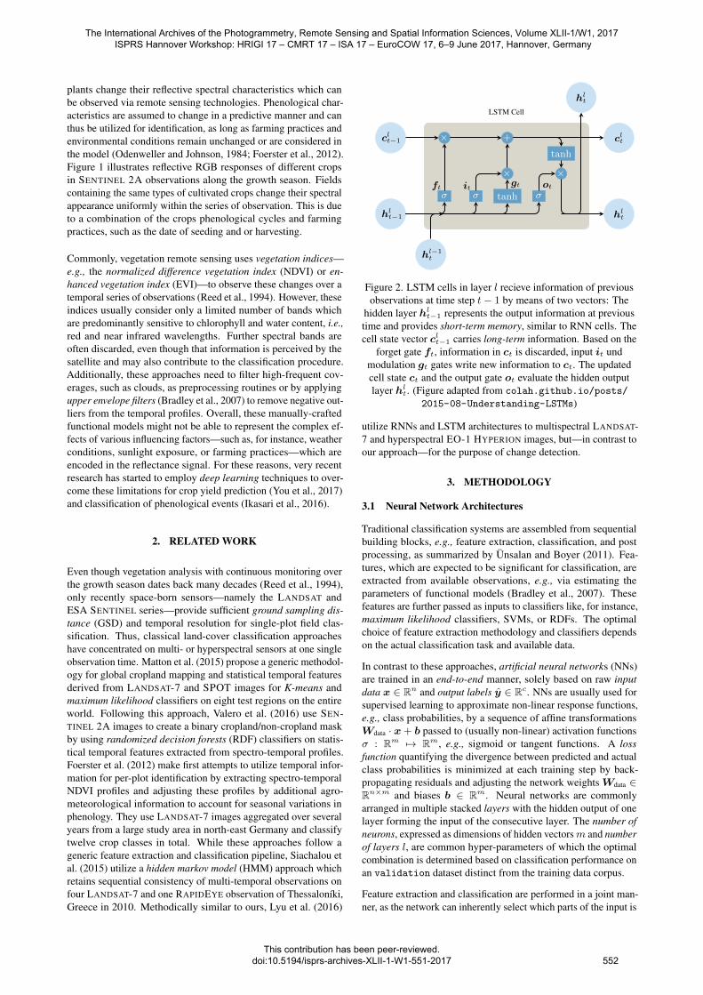
Figure 2. LSTM cells in layer l recieve information of previousobservations at time step t− 1 by means of two vectors: The

hidden layer hlt−1 represents the output information at previous

time and provides short-term memory, similar to RNN cells. Thecell state vector clt−1 carries long-term information. Based on the

forget gate ft, information in ct is discarded, input it undmodulation gt gates write new information to ct. The updatedcell state ct and the output gate ot evaluate the hidden outputlayer hl

t. (Figure adapted from colah.github.io/posts/

2015-08-Understanding-LSTMs)

utilize RNNs and LSTM architectures to multispectral LANDSAT-7 and hyperspectral EO-1 HYPERION images, but—in contrast toour approach—for the purpose of change detection.

3. METHODOLOGY

3.1 Neural Network Architectures

Traditional classification systems are assembled from sequentialbuilding blocks, e.g., feature extraction, classification, and postprocessing, as summarized by Unsalan and Boyer (2011). Fea-tures, which are expected to be significant for classification, areextracted from available observations, e.g., via estimating theparameters of functional models (Bradley et al., 2007). Thesefeatures are further passed as inputs to classifiers like, for instance,maximum likelihood classifiers, SVMs, or RDFs. The optimalchoice of feature extraction methodology and classifiers dependson the actual classification task and available data.

In contrast to these approaches, artificial neural networks (NNs)are trained in an end-to-end manner, solely based on raw inputdata x ∈ Rn and output labels y ∈ Rc. NNs are usually used forsupervised learning to approximate non-linear response functions,e.g., class probabilities, by a sequence of affine transformationsWdata · x+ b passed to (usually non-linear) activation functionsσ : Rm 7→ Rm, e.g., sigmoid or tangent functions. A lossfunction quantifying the divergence between predicted and actualclass probabilities is minimized at each training step by back-propagating residuals and adjusting the network weightsWdata ∈Rn×m and biases b ∈ Rm. Neural networks are commonlyarranged in multiple stacked layers with the hidden output of onelayer forming the input of the consecutive layer. The number ofneurons, expressed as dimensions of hidden vectorsm and numberof layers l, are common hyper-parameters of which the optimalcombination is determined based on classification performance onan validation dataset distinct from the training data corpus.

Feature extraction and classification are performed in a joint man-ner, as the network can inherently select which parts of the input is


This contribution has been peer-reviewed. doi:10.5194/isprs-archives-XLII-1-W1-551-2017

552

colah.github.io/posts/2015-08-Understanding-LSTMs

colah.github.io/posts/2015-08-Understanding-LSTMs

x1

t1

LSTM

softmax

y1

H1(y1,y1)

y1

x2

t2

LSTM

softmax

y2

H2(y2,y2)

y2

x3

t3

LSTM

softmax

y3

H3(y3,y3)

y3

input data xt:

day of observation ttand raster reflectances ρt

network

predicted classprobabilities yt

cross entropy loss

reference classprobabilities yt

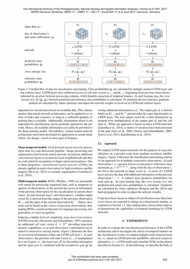
Figure 3. Unrolled flow of data for classification and training. Class probabilities yt are calculated by multiple stacked LSTM layers andone softmax layer. LSTM layers have additional access to cell state vectors ct−1 and ht−1 originating from previous observations,indicated by an arrow between processing columns, which benefits extraction of temporal features. At each training step, the crossentropy loss Ht(yt,yt) between predicted and reference class probabilites is calculated. To minimize the loss function, gradients

(dotted) are calculated by Adam optimizer and adjust the network weights in involved in LSTM and softmax layers.

important for classification based on available data. This schemeensures that neural network architectures can be applied to a va-riety of tasks and scenarios, as long as a sufficient quantity oftraining data is available. Additionally, information which is notimportant for classification can be gradually ignored by the net-work. Hence, all available information can safely be provided tothe deep learning model. Nevertheless, various neural networkarchitectures have been developed for application to certain fieldswhich—by design—excel at some types of features.

Mono-temporal models Feed-forward neural networks processinput data in a one-directional pipeline. Image processing andsegmentation feed forward neural networks incorporate additionalconvolutional layers to account for local neighborhoods and thusare well suited for recognition of shapes and textural patterns. Dueto these properties, convolutional neural networks (CNNs) arealready applied in earth observation for high resolution satelliteimagery (Hu et al., 2015) or semantic segmentation (Castelluccioet al., 2015).

Multi-temporal models RNNs (Werbos, 1990) are potentiallywell suited for processing sequential data, such as temporal se-quences of observations, as the network has access to informationof the previous observation for the classification of current obser-vation. At each network layer l and observation t, a hidden outputvector hl

t is derived from the output of the previous observationhl

t−1 and the input of the current observation hl−1t . Hence, deci-

sions can be based on the context of previous observations, thusmaking RNNs a useful architecture for language processing, textgeneration, or voice recognition.

Inducing a further level of complexity, long short-term memory(LSTM) networks (Hochreiter and Schmidhuber, 1997) introducean additional cell state vector clt ∈ Rm providing long-termmemory capabilities, as at each observation t information can bestored or retrieved to varying extents. Figure 2 illustrates the flowof vectorized information within one LSTM cell layer l. At eachobservation t, the previous cell state vector clt−1 is manipulatedby a set of gates, i.e., the forget gate f l

t for discarding informationand the input gate ilt combined with the modulation gate glt for

writing additional information to clt. The output gate olt is derivedbased on hl

t−1 and hl−1t and provides the same functionality as

a RNN layer. The new output vector hlt is then obtained by an

element-wise multiplication of the output gate olt and the cellstate clt. While our approach is based on these LSTM networks(Zaremba et al., 2014), a variety of variations have been presentedin the past (Gers et al., 2002; Graves and Schmidhuber, 2005;Graves et al., 2013; Kalchbrenner et al., 2015).

3.2 Approach

We employ LSTM neural networks for the purpose of crop clas-sification on a per-plot scale from medium resolution satelliteimagery. Figure 3 illustrates the classification and training schemeof our approach for at multiple consecutive observations. At eachobservation t, ns spectral bottom-of-atmosphere reflectance mea-surements ρi ∈ R(k×k)·ns , along with the day of observation tiare fed to the network as input vector x. A series of l LSTMlayers process the data with additional information of the previousobservation t − 1. A softmax layer produces probabilities foreach class yt. At each training step, the cross-entropy loss wrt.predicted and actual class probabilities is calculated. Gradientsare calculated by Adam optimizer (Kingma and Ba, 2014) andback-propagated in order to adjust the network weights.

Crops have been chosen as subject of classification since these landcover classes are expected to change in a characteristic manner, asexplained in Section 1.1, thus making these classes ideal subjectsto demonstrate the capabilities of temporal modeling by LSTMnetworks.

4. EXPERIMENTS

In order to evaluate the classification performance of the LSTMarchitecture and to investigate the effects of temporal features onthe classification results, we trained multiple multi-temporal mod-els, i.e., based on LSTM networks and RNNs, and mono-temporalalternatives, i.e., a CNN model and a baseline SVM, on the datasetdescribed in Section 4.1. In the following, we describe the body of



553

Figure 4. In our experiments, we used an area of interest of102 km× 42 km (black rectangle) in the north of Munich,

Germany, as study area containing 137 k field plots.

obtained data in Section 4.1 and the performed data aggregation toobtain input and label vectors in Section 4.2. Section 4.3 explainsthe intuitions behind the different dataset partitioning regimesto obtain training, validation, and evaluation subsets inthe context of phenological temporal features and regional en-vironmental influences. The training and evaluation process isexplained in Section 4.4 and results are shown in Section 4.5.

4.1 Data Material

To train the large number of neural network weights, a feasiblebody of raster and label data is necessary. For this reason a largearea of interest (AOI) of 102 km× 42 km in the north of Munich,Germany, has been selected (cf. Figure 4) due to its homogeneousgeography, climate conditions, and farming practices which sug-gest similar environmental conditions. A raster dataset of 26SENTINEL 2A images, acquired between 31st December, 2015and 30th September, 2016, has been retrieved from ESA SCI-HUB and atmospherically corrected by SEN2COR software. Forconsistency reasons with the LANDSAT series, blue, green, red,near-infrared and shortwave infrared 1 and 2 bands were selectedfor this evaluation. Field geometries and cultivated crop labels of137 k fields in the AOI have been provided by the Bavarian Min-istry of Agriculture (Bayrische Staatsministerium fur Ernahrung,Landwirtschaft und Forsten).

The distribution of fields per crop class is not uniform with com-mon cultivated crops, e.g., corn or wheat, dominating the dataset,while other crops, e.g., sugar beet or asparagus, are less repre-sented (cf. Figure 5). Nevertheless, from 172 unique field crops,19 field classes have been selected with at least 400 field-plots inthe AOI.

4.2 Data Extraction

The field geometries of the field and reflection values of theraster dataset have been discretized to a 100m× 100m gridof points of interest (POIs). Each POI contains information ofnetwork input x and classification ground truth labels y in a30m× 30m neighborhood. The network input vector x incor-porated bottom-of-atmosphere reflection values directly derivedfrom the raster dataset combined with the day of observation

othercorn

meadow

aspara

gusrap

ehop

summer oats

winterspelt

fallow

winterwheat

winterbarl

ey

winterrye

beans

wintertrit

icale

summer barleypeas

potatoe

soybeans

sugar beets

0.001

0.01

0.1

crop class

freq

uenc

y

Training examples Testing examples

Figure 5. Distribution of classes by fields in the AOI. Commonfield crops, such as corn or wheat, dominate the dataset with 28k

and 22k fields, respectively, while, e.g., asparagus or peas arecultivated in less than 600 fields. Only crops with at least 400

occurances have been included in the dataset.

normalized as fraction of year. The network labels y have beenformed by two types of classes.

1. Field classes were derived from the field dataset, namelycorn, meadow, asparagus, rape, hop, summer oats, winterspelt, fallow, winter wheat, winter barley, winter rye, beans,winter triticale, summer barley, peas, potatoe, sugar beets,soybeans, and the default class other.

2. Covered classes cloud, water, snow, and cloud shadow, ac-count for high frequent coverages and are provided by thescene classification mask of SEN2COR extracted from theraster dataset.

If POIs were located at the border of multiple classes, class labelshave been weighted with respect to a local 30m neighborhood.

4.3 Dataset Partitioning

Commonly, two sets of parameters need to be determined whenselecting and training the neural network architecture. WeightsW ∈ Rn×m are adjusted during the training process by back-propagation of residuals and hyper-parameters θ are chosen fol-lowing a grid search regime in order to find the optimal networkstructure for the classification task. To ensure that these param-eters are chosen independently, training of network weights andevaluation of hyper-parameters was performed on training andvalidation datasets, respectively. A third evaluation datasetis used for to calculate accuracy measures of neural networkindependently from network weights and parameters. Whilethe evaluation dataset remained unchanged, training andvalidation were redistributed in multiple folds. This practicemaximizes the number of training samples and avoids misrepre-sentations of classes containing small numbers of features in therespective dataset. Hence, the body of POIs was divided in thethree respective datasets.

As discussed in Section 1.1, the dates of phenological events areinfluenced by environmental conditions which vary at large spatialdistances. To average these environmental conditions, the body ofdata is divided randomly with respect to the extent of the AOI. Apure random assignment of individual POIs would ensure an evendistribution of POIs but may assign POIs of the same field to thedifferent datasets and thus cause dependencies between datasets.

For these reasons, the POIs were not assigned completely ran-domly to the respective datasets, but have been first partitioned in



554

Figure 6. Illustration of the field dataset overlayed with3 km× 3 km blocks dedicated for training (blue),evaluation (lightblue), and validation (orange). A

circumferential margin of 200m ensures that field plots are notlocated in two distinct datasets. Training and evaluation

datasets are randomly reassigned at each cross-validation fold.

blocks. These 476 blocks of 3 km× 3 km were in turn randomlyassigned to training, validation, and evaluation in a 4:1:1ratio (cf. Figure 6). A circumferential margin of 200m ensuresthat POIs located on the same field were not assigned to differ-ent datasets. At each fold, training and evaluation blocksgot reassigned randomly while the validation dataset remainedunchanged.

4.4 Experimental Setup

In total, 135 networks of each architecture have been trainedthe body of training data over 30 epochs with varying hyper-parameters l ∈ {2, 3, 4} and r ∈ {110, 220, 330, 440, 880}.This process has been repeated in 9 folds of randomly reassignedtraining and validation datasets. Dropout with probabilitypdropout = 0.5 was used for regularization. Additional to the inves-tigated neural network architectures, a baseline SVM with radialbasis function (RBF) kernel was trained on a balanced datasetof 3,000 samples per class extracted from the training dataset.The optimal hyper-parameters, i.e., slack penalty C and RBFscaling factor γ, have been chosen based on a grid search overC ∈

{10−2, ..., 106

}and γ ∈

{10−2, ..., 103

}. All networks

have been trained within 8 hours on a NVIDIA DGX-1 serverequipped with eight NVIDIA TESLA P100 GPUs and 16GBVRAM each. Five networks have been able to be trained on eachGPU in parallel, making the large grid search of parameters possi-ble. While neural networks were implemented in TENSORFLOW,the SVM baseline based on the SCIKIT-LEARN framework.

The best network performances have been achieved by networkswith hyper-parameter settings θLSTM = (l = 4, r = 440), θRNN =(4, 880), and θCNN = (3, 880). The SVM baseline performed bestwith θSVM = (C = 10, γ = 10).

4.5 Results

In this section, we evaluate the performance of the trained net-works at multiple scales from general performance of each neuralnetwork architecture to the performance of best networks on indi-vidual classes.

4.5.1 Training performance Figure 7 shows the overall ac-curacy of each architecture on the validation dataset withinthe training process by means of the average overall accuracy asindication of general performance of the respective architecture.Variations of observed accuracy were presumably caused by the

0 2 4 6

·106

0.5

0.6

0.7

0.8

0.9

training iterations

over

alla

ccur

acy

CNN σ CNN mean CNN bestRNN σ RNN mean RNN bestLSTM σ LSTM mean LSTM best

Figure 7. Evolution of overall validation accuracy performanceduring the training process of 135 networks of each CNN, RNN,and LSTM architecture with different hyperparameter settings.Means (dashed lines) and standard deviation intervals (shaded

areas) indicate the general performance of each architecture, themost performand network is superimposed separately (solid line).

chosen hyper-parameter sets and are indicated by their standarddeviation intervals. These standard deviations turned out to be rel-atively small compared to the performances of LSTM, RNN, andCNN models and suggest that, on this dataset, the choice of the ac-tual architecture has larger influence on classification performancethan the choice of the involved hyper-parameters. Overall, LSTMnetworks and RNNs achieved significantly better accuracies overthe entire training process with LSTM models performing slightlybetter than their RNN competitors. The networks which achievedbest accuracies are plotted separately as solid lines, as these willbe evaluated in detail in the following.

4.5.2 Accuracy measures per best network The best per-forming networks, opposed to the SVM baseline, have been testedin detail on the evaluation dataset. Results of these experimentsare compiled in Table 1. Additionally, covered and field classeshave been separated from each other. Similarly to the previous fig-ure, multi-temporal models achieved better accuracies comparedto mono-temporal competitors. This performance gain is supposedto be largely caused by the field classes which—in contrast to cov-ered classes—contain temporal phenological characteristics likelyto be utilized by LSTMs and RNNs. Covered classes achievedsimilar accuracies in all of the models with also the baseline SVMachieving good classification accuracies. Apparently, the charac-teristics of these classes are more distinctive and can be utilizedby all models.

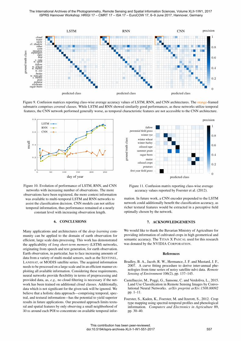
4.5.3 Class confusions Similar results can be observed fromthe confusion matrices shown in Figure 9 based on the best per-forming networks and the SVM baseline shown in Figure 8. Theclass frequencies are normalized by the sum of ground truth classesto obtain the precision measure. While some classes representdistinct cultivated crop, other classes—such as meadow, fallow, orother—can not be defined precisely. Consequently, these classesperformed worse during our experiments and were more likelyconfused with a variety of other classes, as becoming apparentin in the confusion matrix. Further chance for confusion wasobserved in the case of classes with are botanically related to eachother and thus share similar spectral and temporal features. Forinstance, the classes triticale, wheat, and rye have been commonlyconfused, as triticale is a hybrid of the latter two classes. The CNNmodel, in general, performed worse compared to LSTM and RNN.Some classes (e.g., sugar beets, wheat) achieved good accuracies,



555

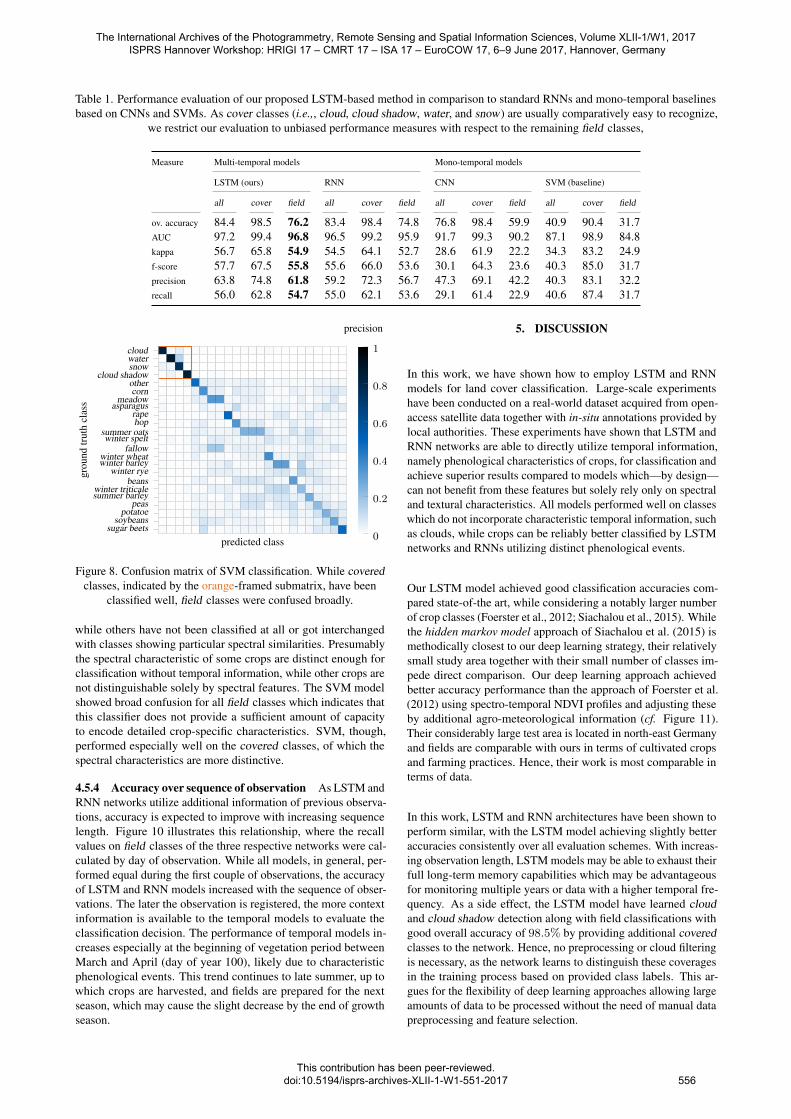
Table 1. Performance evaluation of our proposed LSTM-based method in comparison to standard RNNs and mono-temporal baselinesbased on CNNs and SVMs. As cover classes (i.e.,, cloud, cloud shadow, water, and snow) are usually comparatively easy to recognize,

we restrict our evaluation to unbiased performance measures with respect to the remaining field classes,

Measure Multi-temporal models Mono-temporal models

LSTM (ours) RNN CNN SVM (baseline)

all cover field all cover field all cover field all cover field

ov. accuracy 84.4 98.5 76.2 83.4 98.4 74.8 76.8 98.4 59.9 40.9 90.4 31.7AUC 97.2 99.4 96.8 96.5 99.2 95.9 91.7 99.3 90.2 87.1 98.9 84.8kappa 56.7 65.8 54.9 54.5 64.1 52.7 28.6 61.9 22.2 34.3 83.2 24.9f-score 57.7 67.5 55.8 55.6 66.0 53.6 30.1 64.3 23.6 40.3 85.0 31.7precision 63.8 74.8 61.8 59.2 72.3 56.7 47.3 69.1 42.2 40.3 83.1 32.2recall 56.0 62.8 54.7 55.0 62.1 53.6 29.1 61.4 22.9 40.6 87.4 31.7

cloudwatersnow

cloud shadowothercorn

meadowasparagus

rapehop

summer oatswinter spelt

fallowwinter wheatwinter barley

winter ryebeans

winter triticalesummer barley

peaspotatoe

soybeanssugar beets

predicted class

grou

ndtr

uth

clas

s

0

0.2

0.4

0.6

0.8

1

precision

Figure 8. Confusion matrix of SVM classification. While coveredclasses, indicated by the orange-framed submatrix, have been

classified well, field classes were confused broadly.

while others have not been classified at all or got interchangedwith classes showing particular spectral similarities. Presumablythe spectral characteristic of some crops are distinct enough forclassification without temporal information, while other crops arenot distinguishable solely by spectral features. The SVM modelshowed broad confusion for all field classes which indicates thatthis classifier does not provide a sufficient amount of capacityto encode detailed crop-specific characteristics. SVM, though,performed especially well on the covered classes, of which thespectral characteristics are more distinctive.

4.5.4 Accuracy over sequence of observation As LSTM andRNN networks utilize additional information of previous observa-tions, accuracy is expected to improve with increasing sequencelength. Figure 10 illustrates this relationship, where the recallvalues on field classes of the three respective networks were cal-culated by day of observation. While all models, in general, per-formed equal during the first couple of observations, the accuracyof LSTM and RNN models increased with the sequence of obser-vations. The later the observation is registered, the more contextinformation is available to the temporal models to evaluate theclassification decision. The performance of temporal models in-creases especially at the beginning of vegetation period betweenMarch and April (day of year 100), likely due to characteristicphenological events. This trend continues to late summer, up towhich crops are harvested, and fields are prepared for the nextseason, which may cause the slight decrease by the end of growthseason.

5. DISCUSSION

In this work, we have shown how to employ LSTM and RNNmodels for land cover classification. Large-scale experimentshave been conducted on a real-world dataset acquired from open-access satellite data together with in-situ annotations provided bylocal authorities. These experiments have shown that LSTM andRNN networks are able to directly utilize temporal information,namely phenological characteristics of crops, for classification andachieve superior results compared to models which—by design—can not benefit from these features but solely rely only on spectraland textural characteristics. All models performed well on classeswhich do not incorporate characteristic temporal information, suchas clouds, while crops can be reliably better classified by LSTMnetworks and RNNs utilizing distinct phenological events.

Our LSTM model achieved good classification accuracies com-pared state-of-the art, while considering a notably larger numberof crop classes (Foerster et al., 2012; Siachalou et al., 2015). Whilethe hidden markov model approach of Siachalou et al. (2015) ismethodically closest to our deep learning strategy, their relativelysmall study area together with their small number of classes im-pede direct comparison. Our deep learning approach achievedbetter accuracy performance than the approach of Foerster et al.(2012) using spectro-temporal NDVI profiles and adjusting theseby additional agro-meteorological information (cf. Figure 11).Their considerably large test area is located in north-east Germanyand fields are comparable with ours in terms of cultivated cropsand farming practices. Hence, their work is most comparable interms of data.

In this work, LSTM and RNN architectures have been shown toperform similar, with the LSTM model achieving slightly betteraccuracies consistently over all evaluation schemes. With increas-ing observation length, LSTM models may be able to exhaust theirfull long-term memory capabilities which may be advantageousfor monitoring multiple years or data with a higher temporal fre-quency. As a side effect, the LSTM model have learned cloudand cloud shadow detection along with field classifications withgood overall accuracy of 98.5% by providing additional coveredclasses to the network. Hence, no preprocessing or cloud filteringis necessary, as the network learns to distinguish these coveragesin the training process based on provided class labels. This ar-gues for the flexibility of deep learning approaches allowing largeamounts of data to be processed without the need of manual datapreprocessing and feature selection.



556

cloudwatersnow

cl. shadowothercorn

meadowasparagusrapehop

s. oatsw. speltfallow

w. wheatw. barleyw. ryebeans

w. triticales. barleypeas

potatoesoybeans

sugar beets

predicted class

grou

ndtr

uth

clas

s

LSTM

predicted class

RNN

predicted class

CNN

0

0.2

0.4

0.6

0.8

1

precision

Figure 9. Confusion matrices reporting class-wise average accuracy values of LSTM, RNN, and CNN architectures. The orange-framedsubmatrix comprises covered classes. While LSTM and RNN showed similarily good performances, as these networks utilize temporalfeatures, the CNN network performed generally worse, as temporal characteristic features are not accessible to the CNN architecture.

0 50 100 150 200 2500

0.2

0.4

0.6

0.8

day of year

reca

ll

LSTMRNNCNN

Figure 10. Evolution of performance of LSTM, RNN, and CNNnetworks with increasing number of observations. The more

observations have been registered, the more context informationwas available to multi-temporal LSTM and RNN networks toassist the classification decision. CNN models can not utilizetemporal information, thus performance remained at a nearly

constant level with increasing observation length.

6. CONCLUSIONS

Many applications and architectures of the deep learning com-munity can be applied to the domain of earth observation forefficient, large scale data processing. This work has demonstratedthe applicability of long short-term memory (LSTM) networks,originating from speech and text generation, for earth observation.Earth observation, in particular, has to face increasing amounts ofdata from a variety of multi-modal sensors, such as the SENTINEL,LANDSAT, or MODIS satellite series. The acquired informationneeds to be processed on a large scale and in an efficient manner ex-ploiting all available information. Considering these requirements,neural networks provide flexibility in terms of preprocessing andprovided data, as, e.g., no cloud filtering is necessary if the net-work has been trained on additional cloud classes. Additionally,data which is not significant for the given task will be ignored. Webelieve that a holistic data approach—comprising temporal, spec-tral, and textural information—has the potential to yield superiorresults in future applications. Our presented approach limits textu-ral and spatial features by only observing a small neighborhood of30m around each POI to concentrate on available temporal infor-

fallowperennial field grass

winter rye

winter wheatwinter barleyoilseed rape

summer grainsugar beets

maizeoilseed crops

potatoesfirst year field grass

predicted class

grou

ndtr

uth

clas

s

0

0.2

0.4

0.6

0.8

1

precision

Figure 11. Confusion matrix reporting class-wise averageaccuracy values reported by Foerster et al. (2012).

mation. In future work, a CNN encoder prepended to the LSTMnetwork could additionally benefit the classification accuracy, asricher textural features would be extracted in a perceptive fieldoptimally chosen by the network.

7. ACKNOWLEDGEMENTS

We would like to thank the Bavarian Ministry of Agriculture forproviding information of cultivated crops in high geometrical andsemantic accuracy. The TITAN X PASCAL used for this researchwas donated by the NVIDIA CORPORATION.

References

Bradley, B. A., Jacob, R. W., Hermance, J. F. and Mustard, J. F.,2007. A curve fitting procedure to derive inter-annual phe-nologies from time series of noisy satellite ndvi data. RemoteSensing of Environment 106(2), pp. 137–145.

Castelluccio, M., Poggi, G., Sansone, C. and Verdoliva, L., 2015.Land Use Classification in Remote Sensing Images by Convo-lutional Neural Networks. arXiv preprint arXiv:1508.00092pp. 1–11.

Foerster, S., Kaden, K., Foerster, M. and Itzerott, S., 2012. Croptype mapping using spectral-temporal profiles and phenologicalinformation. Computers and Electronics in Agriculture 89,pp. 30–40.



557

Gers, F. A., Schraudolph, N. N. and Schmidhuber, J., 2002. Learn-ing precise timing with lstm recurrent networks. Journal ofmachine learning research 3(Aug), pp. 115–143.

Graves, A. and Schmidhuber, J., 2005. Framewise phonemeclassification with bidirectional lstm and other neural networkarchitectures. Neural Networks 18(5), pp. 602–610.

Graves, A., Mohamed, A.-r. and Hinton, G., 2013. Speech recogni-tion with deep recurrent neural networks. In: Acoustics, speechand signal processing (icassp), 2013 ieee international confer-ence on, IEEE, pp. 6645–6649.

Hochreiter, S. and Schmidhuber, J., 1997. Long Short-TermMemory. Neural Computation 9(8), pp. 1735–1780.

Hu, F., Xia, G.-S., Hu, J. and Zhang, L., 2015. Transferring DeepConvolutional Neural Networks for the Scene Classification ofHigh-Resolution Remote Sensing Imagery. Remote Sensing7(11), pp. 14680–14707.

Ikasari, I. H., Ayumi, V., Fanany, M. I. and Mulyono, S., 2016.Multiple regularizations deep learning for paddy growth stagesclassification from landsat-8. arXiv preprint arXiv:1610.01795.

Kalchbrenner, N., Danihelka, I. and Graves, A., 2015. Grid longshort-term memory. arXiv preprint arXiv:1507.01526.

Kingma, D. and Ba, J., 2014. Adam: A method for stochasticoptimization. arXiv preprint arXiv:1412.6980.

Lyu, H., Lu, H. and Mou, L., 2016. Learning a TransferableChange Rule from a Recurrent Neural Network for Land CoverChange Detection. Remote Sensing 8(6), pp. 1–22.

Matton, N., Canto, G. S., Waldner, F., Valero, S., Morin, D.,Inglada, J., Arias, M., Bontemps, S., Koetz, B. and Defourny,P., 2015. An Automated Method for Annual Cropland Mappingalong the Season for Various Globally-Distributed Agrosys-tems Using High Spatial and Temporal Resolution Time Series.Remote Sensing 7(10), pp. 13208–13232.

Odenweller, J. B. and Johnson, K. I., 1984. Crop identificationusing landsat temporal-spectral profiles. Remote Sensing ofEnvironment 14(1-3), pp. 39–54.

Reed, B. C., Brown, J. F., VanderZee, D., Loveland, T. R., Mer-chant, J. W. and Ohlen, D. O., 1994. Measuring Phenologi-cal Variability from Satellite Imagery. Journal of VegetationScience, 5(5), 703–714. http://doi.org/10.2307/3235884suringPhenologica. Journal of Vegetation Science 5(5), pp. 703–714.

Siachalou, S., Mallinis, G. and Tsakiri-Strati, M., 2015. A HiddenMarkov Models Approach for Crop Classification: LinkingCrop Phenology to Time Series of Multi-Sensor Remote Sens-ing Data. Remote Sensing 7(4), pp. 3633–3650.

Unsalan, C. and Boyer, K. L., 2011. Review on Land Use Classifi-cation. In: Multispectral Satellite Image Understanding: FromLand Classification to Building and Road Detection, Springer,pp. 49–64.

Valero, S., Morin, D., Inglada, J., Sepulcre, G., Arias, M., Hagolle,O., Dedieu, G., Bontemps, S., Defourny, P. and Koetz, B., 2016.Production of a Dynamic Cropland Mask by Processing RemoteSensing Image Series at High Temporal and Spatial Resolutions.Remote Sensing 8(1), pp. 1–21.

Werbos, P. J., 1990. Backpropagation through time: what it doesand how to do it. Proceedings of the IEEE 78(10), pp. 1550–1560.

Whitcraft, A. K., Becker-Reshef, I. and Justice, C. O., 2014. Agri-cultural growing season calendars derived from MODIS surfacereflectance. International Journal of Digital Earth 8(3), pp. 173–197.

You, J., Li, X., Low, M., Lobell, D. and Ermon, S., 2017. Deepgaussian process for crop yield prediction based on remotesensing data.

Zaremba, W., Sutskever, I. and Vinyals, O., 2014. Recurrent neuralnetwork regularization. arXiv preprint arXiv:1409.2329.


This contribution has been peer-reviewed. doi:10.5194/isprs-archives-XLII-1-W1-551-2017 558

multi-temporal land cover classification with long … · key words: long short-term memory,...

Documents