multi-state modelling with r: the msm package -...

Multi-state modelling with R: the msm package

Version 0.6.3

Christopher JacksonDepartment of Epidemiology and Public Health

Imperial College, London

[email protected]

Abstract

The multi-state Markov model is a useful way of describing a process in which an individualmoves through a series of states in continuous time. The msm package for R allows a generalmulti-state model to be fitted to longitudinal data. Data often consist of observations of the processat arbitrary times, so that the exact times when the state changes are unobserved. For example,the progression of chronic diseases is often described by stages of severity, and the state of thepatient may only be known at doctor or hospital visits. Features of msm include the ability tomodel transition rates and hidden Markov output models in terms of covariates, and the ability tomodel data with a variety of observation schemes, including censoring.

Hidden Markov models, in which the true path through states is only observed through someerror-prone marker, can also be fitted. The observation is generated, conditionally on the underly-ing states, via some distribution. An example is a screening misclassification model in which statesare observed with error. More generally, hidden Markov models can have a continuous response,with some arbitrary distribution, conditionally on the underlying state.

This manual introduces the theory behind multi-state Markov and hidden Markov models, andgives a tutorial in the typical use of the msm package, illustrated by some typical applications tomodelling chronic diseases.

Contents1 Multi-state models 3

1.1 Introduction . . . . . . . . . . . . . . . . . . . . . . . . . . . . . . . . . . . . . . . 31.2 Disease progression models . . . . . . . . . . . . . . . . . . . . . . . . . . . . . . . 31.3 Arbitrary observation times . . . . . . . . . . . . . . . . . . . . . . . . . . . . . . . 31.4 Likelihood for the multi-state model . . . . . . . . . . . . . . . . . . . . . . . . . . 51.5 Covariates . . . . . . . . . . . . . . . . . . . . . . . . . . . . . . . . . . . . . . . . 111.6 Hidden Markov models . . . . . . . . . . . . . . . . . . . . . . . . . . . . . . . . . 11

1.6.1 Misclassification models . . . . . . . . . . . . . . . . . . . . . . . . . . . . 121.6.2 General hidden Markov model . . . . . . . . . . . . . . . . . . . . . . . . . 131.6.3 Likelihood for general hidden Markov models . . . . . . . . . . . . . . . . . 131.6.4 Example of a general hidden Markov model . . . . . . . . . . . . . . . . . . 14

1

2 Fitting multi-state models with msm 162.1 Installing msm . . . . . . . . . . . . . . . . . . . . . . . . . . . . . . . . . . . . . . 162.2 Getting the data in . . . . . . . . . . . . . . . . . . . . . . . . . . . . . . . . . . . . 162.3 Specifying a model . . . . . . . . . . . . . . . . . . . . . . . . . . . . . . . . . . . 182.4 Specifying initial values . . . . . . . . . . . . . . . . . . . . . . . . . . . . . . . . . 182.5 Running msm . . . . . . . . . . . . . . . . . . . . . . . . . . . . . . . . . . . . . . 192.6 Showing results . . . . . . . . . . . . . . . . . . . . . . . . . . . . . . . . . . . . . 202.7 Covariates on the transition rates . . . . . . . . . . . . . . . . . . . . . . . . . . . . 202.8 Fixing parameters at their initial values . . . . . . . . . . . . . . . . . . . . . . . . . 232.9 Extractor functions . . . . . . . . . . . . . . . . . . . . . . . . . . . . . . . . . . . 232.10 Survival plots . . . . . . . . . . . . . . . . . . . . . . . . . . . . . . . . . . . . . . 262.11 Convergence failure . . . . . . . . . . . . . . . . . . . . . . . . . . . . . . . . . . . 272.12 Model assessment . . . . . . . . . . . . . . . . . . . . . . . . . . . . . . . . . . . . 282.13 Fitting misclassification models with msm . . . . . . . . . . . . . . . . . . . . . . . 302.14 Effects of covariates on misclassification rates . . . . . . . . . . . . . . . . . . . . . 322.15 Extractor functions . . . . . . . . . . . . . . . . . . . . . . . . . . . . . . . . . . . 332.16 Recreating the path through underlying states . . . . . . . . . . . . . . . . . . . . . 352.17 Fitting general hidden Markov models with msm . . . . . . . . . . . . . . . . . . . 36

2.17.1 Defining a new hidden Markov model distribution . . . . . . . . . . . . . . 45

3 msm reference guide 47

A Changes in the msm package 47

2

1 Multi-state models

1.1 IntroductionFigure 1 illustrates a multi-state model in continuous time. Its four states are labelled 1, 2, 3, 4. At atime t the individual is in state S(t). The arrows show which transitions are possible between states.The next state to which the individual moves, and the time of the change, are governed by a set oftransition intensities qrs(t, z(t)) for each pair of states r and s. The intensities may also depend onthe time of the process t, or more generally a set of individual-specific or time-varying explanatoryvariables z(t). The intensity represents the instantaneous risk of moving from state r to state s:

qrs(t, z(t)) = limδt→0

P (S(t + δt) = s|S(t) = r)/δt (1)

The intensities form a matrix Q whose rows sum to zero, so that the diagonal entries are defined byqrr = −

∑s 6=r qrs. To fit a multi-state model to data, we estimate this transition intensity matrix. We

concentrate on Markov models here. The Markov assumption is that future evolution only dependson the current state. That is, qrs(t, z(t),Ft) is independent of Ft, the observation history Ft of theprocess up to the time preceding t. See, for example, Cox and Miller[1] for a thorough introductionto the theory of continuous-time Markov chains.

1.2 Disease progression modelsThe development of the msm package was motivated by applications to disease modelling. Manychronic diseases have a natural interpretation in terms of staged progression. Multi-state Markovmodels in continuous time are often used to model the course of diseases. A commonly-used modelis illustrated in Figure 2. This represents a series of successively more severe disease stages, and an‘absorbing’ state, often death. The patient may advance into or recover from adjacent disease stages,or die at any disease stage. Observations of the state Si(t) are made on a number of individuals i atarbitrary times t, which may vary between individuals. The stages of disease may be modelled as ahomogeneous continuous-time Markov process, with a transition matrix Q, pictured below Figure 2.

A commonly-used model is the illness-death model, with three states representing health, illnessand death (Figure 3). Transitions are permitted from health to illness, illness to death and health todeath. Recovery from illness to health is sometimes also considered.

A wide range of medical situations have been modelled using multi-state methods, for exam-ple, screening for abdominal aortic aneurysms (Jackson et al.[2]), problems following lung trans-plantation (Jackson and Sharples[3]), problems following heart transplantation (Sharples[4], Klotzand Sharples[5]), hepatic cancer (Kay[6]), HIV infection and AIDS (Longini et al.[7], Satten andLongini[8], Guihenneuc-Jouyaux et al.[9], Gentleman et al.[10]), diabetic complications (Marshalland Jones[11], Andersen[12]), breast cancer screening (Duffy and Chen[13], Chen et al.[14]), cer-vical cancer screening (Kirby and Spiegelhalter[15]) and liver cirrhosis (Andersen et al.[16]). Manyof these references also describe the mathematical theory, which will be reviewed in the followingsections.

1.3 Arbitrary observation timesLongitudinal data from monitoring disease progression are often incomplete in some way. Usuallypatients are seen at intermittent follow-up visits, at which monitoring information is collected, but

3

3 4

21

Q =

q11 q12 q13 q14

q21 q22 q23 q24

q31 q32 q33 q34

q41 q42 q43 q44

Figure 1: General multi-state model.

STAGE n−2 STAGE n−1

DISEASE DISEASE DISEASE DISEASE...

ABSORBING

STATE n

STAGE 1 STAGE 2

Q =

q11 q12 0 0 . . . q1n

q21 q22 q23 0 . . . q2n

0 q32 q33 q34. . . q3n

0 0 q43 q44. . . q4n

......

. . . . . . . . ....

0 0 0 0 . . . 0

Figure 2: General model for disease progression.

4

information from the periods between visits is not available. Often the exact time of disease onset isunknown. Thus, the changes of state in a multi-state model usually occur at unknown times. Also asubject may only be followed up for a portion of their disease history. A fixed observation schedulemay be specified in advance, but in practice times of visits may vary due to patient and hospitalpressures. The states of disease progression models often include death. Death times are commonlyrecorded to within a day. Also observations may be censored. For example, at the end of a study, anindividual may be known only to be alive, and in an unknown state.

A typical sampling situation is illustrated in Figure 4. The individual is observed at four occasionsthrough 10 months. The final occasion is the death date which is recorded to within a day. The onlyother information available is the occupation of states 2, 2, and 1 at respective times 1.5, 3.5 and 5.The times of movement between states and the state occupancy in between the observation times areunknown. Although the patient was in state 3 between 7 and 9 months this was not observed at all.

Informative sampling times To fit a model to longitudinal data with arbitrary sampling times wemust consider the reasons why observations were made at the given times. This is analogous to theproblem of missing data, where the fact that a particular observation is missing may implicitly giveinformation about the value of that observation. Possible observation schemes include:

• fixed. Each patient is observed at fixed intervals specified in advance.

• random. The sampling times vary randomly, independently of the current state of the disease.

• doctor’s care. More severely ill patients are monitored more closely. The next sampling timeis chosen on the basis of the current disease state.

• patient self-selection. A patient may decide to visit the doctor on occasions when they are in apoor condition.

Grüger et al. [17] discussed conditions under which sampling times are informative. If a multi-state model is fitted, ignoring the information available in the sampling times, then inference maybe biased. Mathematically, because the sampling times are often themselves random, they shouldbe modelled along with the observation process Xt. However the ideal situation is where the jointlikelihood for the times and the process is proportional to the likelihood obtained if the samplingtimes were fixed in advance. Then the parameters of the process can be estimated independently ofthe parameters of the sampling scheme.

In particular, they showed that fixed, random and doctor’s care observation policies are not infor-mative, whereas patient self-selection is informative.

1.4 Likelihood for the multi-state modelKalbfleisch and Lawless[18] and later Kay [6] described a general method for evaluating the likeli-hood for a general multi-state model in continuous time, applicable to any form of transition matrix.The only available information is the observed state at a set of times, as in Figure 4. The samplingtimes are assumed to be non-informative.

5

DISEASE

FREEDISEASE

DEATH

Figure 3: Illness-death model.

Time

Stage 1

Stage 2

Stage 3

Death

0.0 1.5 3.5 5.0 9.0

Figure 4: Evolution of a multi-state model. The process is observed on four occasions.

6

Transition probability matrix The likelihood is calculated from the transition probability matrixP (t). For a time-homogeneous process, the (r, s) entry of P (t), prs(t), is the probability of beingin state s at a time t + u in the future, given the state at time u is r. It does not say anything aboutthe time of transition from r to s, indeed the process may have entered other states between times uand t + u. P (t) can be calculated by taking the matrix exponential of the scaled transition intensitymatrix (see, for example, Cox and Miller [1]).

P (t) = exp(tQ) (2)

For simpler models, it is feasible to calculate an analytic expression for each element of P (t) interms of Q. This is generally faster and avoids the potential numerical instability of calculating thematrix exponential. Symbolic algebra sofware, such as Mathematica, can be helpful for obtainingthese expressions. For example, the three-state illness-death model with no recovery has a transitionintensity matrix of

Q =

−(q12 + q13) q12 q13

0 −q23 q23

0 0 0

The corresponding time t transition probabilities are

p00(t) = e−(q12+q13)t

p01(t) =

{q12(−1+e(q12+q13−q23)t)e−(q12+q13)t

(q12+q13−q23)(q12 + q13 6= q23)

q12te(−(q12+q13)t (q12 + q13 = q23)

p02(t) =

{1+(−q13+q23)e

−(q12+q13)t

q12+q13−q23− q12e−q23t

q12+q13−q23(q12 + q13 6= q23)

(−1 + e(q12+q13)t − q12t)e−(q12+q13)t (q12 + q13 = q23)

p10(t) = 0p11(t) = e−q23t

p12(t) = 1− e−q23t

p20(t) = 0p21(t) = 0p22(t) = 1

The msm package calculates P (t) analytically for selected 2, 3, 4 and 5-state models. These modelsare illustrated in Figures 5–8. Notice that the states are not labelled in these figures. Each graph cancorrespond to several different Q matrices, depending on how the states are labelled. For example,

Figure 1 a) illustrates the model defined by either Q =(−q12 q12

0 0

)or Q =

(0 0q21 −q21

).

Likelihood for intermittently-observed processes Suppose i indexes M individuals. The data forindividual i consist of a series of times (ti1, . . . , tini) and corresponding states (S(ti1), . . . , S(tini)).Consider a general multi state model, with a pair of successive observed disease states S(tj), S(tj+1)at times tj , tj+1. The contribution to the likelihood from this pair of states is

7

a) b)

Figure 5: Two-state models fitted using analytic P (t) matrices in msm. Implemented for all permu-tations of state labels 1, 2.

a) b)

c) d)

e) f)

Figure 6: Three-state models fitted using analytic P (t) matrices in msm. Implemented for all permu-tations of state labels 1, 2, 3.

8

a)

b)

Figure 7: Four-state models fitted using analytic P (t) matrices in msm. Implemented for all permu-tations of state labels 1, 2, 3, 4.

a)

b)

c)

Figure 8: Five-state models fitted using analytic P (t) matrices in msm. Implemented for all permu-tations of state labels 1, 2, 3, 4, 5.

9

Li,j = pS(tj)S(tj+1)(tj+1 − tj) (3)

This is the entry of the transition matrix P (t) at the S(tj)th row and S(tj+1)th column, evaluated att = tj+1 − tj .

The full likelihood L(Q) is the product of all such terms Li,j over all individuals and all transi-tions. It depends on the unknown transition matrix Q, which was used to determine P (t).

Death states In observational studies of chronic diseases, it is common that the time of death isknown, but the state on the previous instant before death is unknown. If S(tj+1) = D is such a deathstate, then the contribution to the likelihood is summed over the unknown state m on the day beforedeath:

Li,j =∑

m6=D

pS(tj),m(tj+1 − tj)qm,D (4)

assuming a time unit of days. The sum is taken over all possible states m which can be visitedbetween S(tj) and D.

Exactly observed transition times If the times (ti1, . . . , tini) had been the exact transition times

between the states, with no transitions between the observation times, then the contributions wouldbe of the form

Li,j = pS(tj)S(tj)(tj+1 − tj)qS(tj)S(tj+1) (5)

since the state is assumed to be S(tj) throughout the interval between tj and tj+1 with a knowntransition to state S(tj+1) at tj+1.

Censoring At the end of some chronic disease studies, patients are known to be alive but in anunknown state. For such a censored observation S(tj+1), known only to be a state in the set C, theequivalent contribution to the likelihood is

Li,j =∑m∈C

pS(tj),m(tj+1 − tj) (6)

More generally, suppose every observation from a particular individual is censored. Observations1, 2, . . . ni are known only to be in the sets C1, C2, . . . , Cni

respectively. The likelihood for thisindividual is a sum of the likelihoods of all possible paths through the unobserved states.

Li =∑

sni∈Cni

. . .∑

s2∈C2

∑s1∈C1

ps1s2(t2 − t1)ps2s3(t3 − t2) . . . psni−1sni(tni

− tni−1) (7)

Suppose the states comprising the set Cj are c(j)1 , . . . , c

(j)mj . This likelihood can also be written as a

matrix product, say,Li = 1T P 1,2P 2,3 . . . Pni−1,ni1 (8)

where P j−1,j is a mj−1 × mj matrix with (r, s) entry pc(j−1)r c

(j)s

(tj − tj−1), and 1 is the vector ofones.

10

The msm package allows multi-state models to be fitted to data from processes with arbitraryobservation times, exactly-observed transition times, “death” states and censored states, or a mixtureof these schemes.

1.5 CovariatesThe relation of constant or time-varying characteristics of individuals to their transition rates is oftenof interest in a multi-state model. Explanatory variables for a particular transition intensity can beinvestigated by modelling the intensity as a function of these variables. Marshall and Jones [11]described a form of a proportional hazards model, where the transition intensity matrix elements qrs

which are of interest can be replaced by

qrs(z(t)) = q(0)rs exp(βT

rsz(t))

The new Q is then used to determine the likelihood. If the covariates z(t) are time dependent, thecontributions to the likelihood of the form prs(t− u) are replaced by

prs(t− u, z(u))

although this requires that the value of the covariate is known at every observation time u. Sometimescovariates are observed at different times to the main response, for example recurrent disease eventsor other biological markers. In some of these cases it could be assumed that the covariate is a stepfunction which remains constant between its observation times. The msm package allows individual-specific or time dependent covariates to be fitted to transition intensities. Time-dependent covariatesare assumed to be known at the same time as the main response, and constant between observationtimes of the main response.

Marshall and Jones [11] described likelihood ratio and Wald tests for covariate selection andtesting hypotheses, for example whether the effect of a covariate is the same for all forward transitionsin a disease progression model.

1.6 Hidden Markov modelsIn a hidden Markov model (HMM) the states of the Markov chain are not observed. The observeddata are governed by some probability distribution (the emission distribution) conditionally on theunobserved state. The evolution of the underlying Markov chain is governed by a transition intensitymatrix Q as before. (Figure 9). Hidden Markov models are mixture models, where observationsare generated from a certain number of unknown distributions. However the distribution changesthrough time according to states of a hidden Markov chain. This class of model is commonly usedin areas such as speech and signal processing [19] and the analysis of biological sequence data [20].In engineering and biological sequencing applications, the Markov process usually evolves over anequally-spaced, discrete ‘time’ space. Therefore most of the theory of HMM estimation was devel-oped for discrete-time models.

HMMs have less frequently been used in medicine, where continuous time processes are oftenmore suitable. A disease process evolves in continuous time, and patients are often monitored atirregular and differing intervals. These models are suitable for estimating population quantities forchronic diseases which have a natural staged interpretation, but which can only be diagnosed by anerror-prone marker. The msm package can fit continuous-time hidden Markov models with a varietyof emission distributions.

11

Time

ti1 ti2 ti,n−1 ti,n

Underlying

Observed

Si1 Si2 Si,n−1 Si,n

Oi1 Oi2 Oi,n−1 Oi,n

. . .Q

E

Figure 9: A hidden Markov model in continuous time. Observed states are generated conditionallyon an underlying Markov process.

1.6.1 Misclassification models

An example of a hidden Markov model is a multi-state model with misclassification. Here the ob-served data are states, assumed to be misclassifications of the true, underlying states.

For example, consider a disease progression model with at least a disease-free and a disease state.When screening for the presence of the disease, the screening process can sometimes be subject toerror. Then the Markov disease process Si(t) for individual i is not observed directly, but throughrealisations Oi(t). The quality of a diagnostic test is often measured by the probabilities that the trueand observed states are equal, Pr(Oi(t) = r|Si(t) = r). Where r represents a ‘positive’ diseasestate, this is the sensitivity, or the probability that a true positive is detected by the test. Where rrepresents a ‘negative’ or disease-free state, this represents the specificity, or the probability that,given the condition of interest is absent, the test produces a negative result.

As an extension to the simple multi-state model described in section 1, the msm package can fit ageneral multi-state model with misclassification. For patient i, observation time tij , observed statesOij are generated conditionally on true states Sij according to a misclassification matrix E. This is an× n matrix, whose (r, s) entry is

ers = Pr(O(tij) = s|S(tij) = r), (9)

which we first assume to be independent of time t. Analogously to the entries of Q, some of theers may be fixed to reflect knowledge of the diagnosis process. For example, the probability ofmisclassification may be negligibly small for non-adjacent states of disease. Thus the progressionthrough underlying states is governed by the transition intensity matrix Q, while the observationprocess of the underlying states is governed by the misclassification matrix E.

To investigate explanatory variables w(t) for the probability of misclassification ers for each pair

12

of states r and s, a logistic model can be used,

logers(t)

1− ers(t)= γT

rsw(t). (10)

1.6.2 General hidden Markov model

Consider now a general hidden Markov model in continuous time. The true state of the model Sij

evolves as an unobserved Markov process. Observed data yij are generated conditionally true statesSij = 1, 2, . . . , n according to a set of distributions f1(y|θ1, γ1), f2(y|θ2, γ2), . . ., fn(y|θn, γn),respectively. θr is a vector of parameters for the state r distribution. One or more of these parametersmay depend on explanatory variables through a link-transformed linear model with coefficients γr.

1.6.3 Likelihood for general hidden Markov models

A type of EM algorithm known as the Baum-Welch or forward-backward algorithm [21, 22], is com-monly used for hidden Markov model estimation in discrete-time applications. See, for example,Durbin et al.[20], Albert [23]. A generalisation of this algorithm to continuous time was describedby Bureau et al.[24].

The msm package uses a direct method of calculating likelihoods in discrete or continuous timebased on matrix products. This type of method has been described by Macdonald and Zucchini [25,pp. 77–79], Lindsey [26, p.73] and Guttorp [27]. Satten and Longini [8] used this method to calculatelikelihoods for a hidden Markov model in continuous time with observations of a continuous markergenerated conditionally on underlying discrete states.

Patient i’s contribution to the likelihood is

Li = Pr(yi1, . . . , yimi) (11)

=∑

Pr(yi1, . . . , yimi|Si1, . . . , Simi

)Pr(Si1, . . . , Simi)

where the sum is taken over all possible paths of underlying states Si1, . . . , Simi . Assume that theobserved states are conditionally independent given the values of the underlying states. Also assumethe Markov property, Pr(Sij |Si,j−1, . . . , Si1) = Pr(Sij |Si,j−1). Then the contribution Li can bewritten as a product of matrices, as follows. To derive this matrix product, decompose the overallsum in equation 11 into sums over each underlying state. The sum is accumulated over the unknownfirst state, the unknown second state, and so on until the unknown final state:

Li =∑Si1

Pr(yi1|Si1)Pr(Si1)∑Si2

Pr(yi2|Si2)Pr(Si2|Si1)∑Si3

Pr(yi3|Si3)Pr(Si3|Si2)

. . .∑Simi

Pr(yimi|Simi

)Pr(Simi|Sini−1) (12)

where Pr(yij |Sij) is the emission probability density. For misclassification models, this is the mis-classification probability eSijOij

. For general hidden Markov models, this is the probability densityfSij (yij |θSij , γSij ). Pr(Si,j+1|Sij) is the (Sij , Si,j+1) entry of the Markov chain transition matrixP (t) evaluated at t = ti,j+1 − tij . Let f be the vector with r element the product of the initial state

13

occupation probability Pr(Si1 = r) and Pr(yi1|r), and let 1 be a column vector consisting of ones.For j = 2, . . . ,mi let Tij be the n× n matrix with (r, s) entry

Pr(yij |s)prs(tij − ti,j−1)

Then subject i’s likelihood contribution is

Li = fTi2Ti3, . . . Timi1 (13)

If S(tj) = D is an absorbing state such as death, measured without error, whose entry timeis known exactly, then the contribution to the likelihood is summed over the unknown state at theprevious instant before death. the day before entry. The (r, s) entry of Tij is then

prs(tj − tj−1)qs,D

Section 2.13 describes how to fit multi-state models with misclassification using the msm package,and Section 2.17 describes how to apply general hidden Markov models.

1.6.4 Example of a general hidden Markov model

Jackson and Sharples [3] described a model for FEV1 (forced expiratory volume in 1 second) in re-cipients of lung transplants. These patients were at risk of BOS (bronchiolitis obliterans syndrome), aprogressive, chronic deterioration in lung function. In this example, BOS was modelled as a discrete,staged process, a model of the form illustrated in Figure 2, with 4 states. State 1 represents absenceof BOS. State 1 BOS is roughly defined as a sustained drop below 80% below baseline FEV1, whilestate 2 BOS is a sustained drop below 65% baseline. FEV1 is measured as a percentage of a baselinevalue for each individual, determined in the first six months after transplant, and assumed to be 100%baseline at six months.

As FEV1 is subject to high short-term variability due to acute events and natural fluctuations,the exact BOS state at each observation time is difficult to determine. Therefore, a hidden Markovmodel for FEV1, conditionally on underlying BOS states, was used to model the natural history ofthe disease. Discrete states are appropriate as onset is often sudden.

Model 1 Jackson [28] considered models for these data where FEV1 were Normally distributed,with an unknown mean and variance conditionally each state (14). This model seeks the most likelylocation for the within-state FEV1 means.

yij |{Sij = k} ∼ N(µk + βxij , σ2k) (14)

Model 2 Jackson and Sharples [3] used a more complex two-level model for FEV1 measurements.Level 1 (15) represents the short-term fluctuation error of the marker around its underlying continuousvalue yhid

ij . Level 2 (16) represents the distribution of yhidij conditionally on each underlying state, as

follows.yij |yhid

ij ∼ N(yhidij + βxij , σ

2ε ) (15)

14

yhidij |Sij ∼

State Three state model Four state model

Sij = 0 N(µ0, σ20)I[80,∞) N(µ0, σ

20)I[80,∞)

Sij = 1 N(µ1, σ21)I(0,80) Uniform(65, 80)

Sij = 2 (death) N(µ2, σ22)I(0,65)

Sij = 3 (death)

(16)

Integrating over yhidij gives an explicit distribution for yij conditionally on each underlying state

(given in Section 2.17, Table 1). Similar distributions were originally applied by Satten and Longini [8]to modelling the progression through discrete, unobserved HIV disease states using continuous CD4cell counts. The msm package includes density, quantile, cumulative density and random numbergeneration functions for these distributions.

In both models 1 and 2, the term βxij models the short-term fluctuation of the marker in terms ofacute events. xij is an indicator for the occurrence of an acute rejection or infection episode within14 days of the observation of FEV1.

Section 2.17 describes how these and more general hidden Markov models can be fitted with themsm package.

15

2 Fitting multi-state models with msmmsm is a package of functions for multi-state modelling using the R statistical software. The msmfunction itself implements maximum-likelihood estimation for general multi-state Markov or hid-den Markov models in continuous time. We illustrate its use with a set of data from monitoringheart transplant patients. Throughout this section “>” indicates the R command prompt, slantedtypewriter text indicates R commands, and typewriter text R output.

2.1 Installing msmThe easiest way to install the msm package on a computer connected to the Internet is to run the Rcommand:

install.packages("msm")

This downloads msm from the CRAN archive of contributed R packages (cran.r-project.orgor one of its mirrors) and installs it to the default R system library. To install to a different location,for example if you are a normal user with no administrative privileges, create a directory in which Rpackages are to be stored, say, /your/library/dir, and run

install.packages("msm", lib='/your/library/dir')

After msm has been installed, its functions can be made visible in an R session by

> library(msm)

or, if it has been installed into a non-default library,

library(msm, lib.loc='/your/library/dir')

2.2 Getting the data inThe data are specified as a series of observations, grouped by patient. At minimum there should be adata frame with variables indicating

• the time of the observation,

• the observed state of the process.

If the data do not also contain

• the subject identification number,

then all the observations are assumed to be from the same subject. The subject ID does not need tobe numeric, but data must be grouped by subject, and observations must be ordered by time withinsubjects. An example data set, taken from monitoring a set of heart transplant recipients, is providedwith msm. Sharples et al. [29] studied the progression of coronary allograft vasculopathy (CAV), apost-transplant deterioration of the arterial walls, using these data. Risk factors and the accuracy ofthe screening test were investigated using multi-state Markov and hidden Markov models.

This data set can be made available to the current R session by issuing the command

16

> data(heart)

The first three patient histories are shown below. There are 622 patients in all. PTNUM is thesubject identifier. Approximately each year after transplant, each patient has an angiogram, at whichCAV can be diagnosed. The result of the test is in the variable state, with possible values 1,2, 3 representing CAV-free, mild CAV and moderate or severe CAV respectively. A value of 4 isrecorded at the date of death. years gives the time of the test in years since the heart transplant.Other variables include age (age at screen), dage (donor age), sex (0=male, 1=female), pdiag(primary diagnosis, or reason for transplant - IHD represents ischaemic heart disease, IDC representsidiopathic dilated cardiomyopathy), and cumrej (cumulative number of rejection episodes).

> heart[1:21, ]

PTNUM age years dage sex pdiag cumrej state1 100002 52.49589 0.000000 21 0 IHD 0 12 100002 53.49863 1.002740 21 0 IHD 2 13 100002 54.49863 2.002740 21 0 IHD 2 24 100002 55.58904 3.093151 21 0 IHD 2 25 100002 56.49589 4.000000 21 0 IHD 3 26 100002 57.49315 4.997260 21 0 IHD 3 37 100002 58.35068 5.854795 21 0 IHD 3 48 100003 29.50685 0.000000 17 0 IHD 0 19 100003 30.69589 1.189041 17 0 IHD 1 110 100003 31.51507 2.008219 17 0 IHD 1 311 100003 32.49863 2.991781 17 0 IHD 2 412 100004 35.89589 0.000000 16 0 IDC 0 113 100004 36.89863 1.002740 16 0 IDC 2 114 100004 37.90685 2.010959 16 0 IDC 2 115 100004 38.90685 3.010959 16 0 IDC 2 116 100004 39.90411 4.008219 16 0 IDC 2 117 100004 40.88767 4.991781 16 0 IDC 2 118 100004 41.91781 6.021918 16 0 IDC 2 219 100004 42.91507 7.019178 16 0 IDC 2 320 100004 43.91233 8.016438 16 0 IDC 2 321 100004 44.79726 8.901370 16 0 IDC 2 4

A useful way to summarise multi-state data is as a frequency table of pairs of consecutive states.This counts over all individuals, for each state r and s, the number of times an individual had anobservation of state r followed by an observation of state s. The function statetable.msm canbe used to produce such a table, as follows,

> statetable.msm(state, PTNUM, data = heart)

tofrom 1 2 3 4

1 1367 204 44 1482 46 134 54 483 4 13 107 55

17

Thus there were 148 CAV-free deaths, 48 deaths from state 2, and 55 deaths from state 3. On onlyfour occasions was there an observation of severe CAV followed by an observation of no CAV.

2.3 Specifying a modelWe now specify the multi-state model to be fitted to the data. A model is governed by a transitionintensity matrix Q. For the heart transplant example, there are four possible states through whichthe patient can move, corresponding to CAV-free, mild/moderate CAV, severe CAV and death. Weassume that the patient can advance or recover from consecutive states while alive, and die from anystate. Thus the model is illustrated by Figure 2 with four states, and we have

Q =

−(q12 + q14) q12 0 q14

q21 −(q21 + q23 + q24) q23 q24

0 q32 −(q32 + q34) q34

0 0 0 0

It is important to remember that this defines which instantaneous transitions can occur in the

Markov process, and that the data are snapshots of the process (see section 1.3). Although there were44 occasions on which a patient was observed in state 1 followed by state 3, the underlying modelspecifies that the patient must have passed through state 2 in between. If your data represent the exactand complete transition times of the process, then you must specify exacttimes=TRUE in the callto msm.

To tell msm what the allowed transitions of our model are, we define a matrix of the same size asQ, containing zeroes in the positions where the entries of Q are zero. All other positions contain aninitial value for the corresponding transition intensity. The diagonal entries supplied in this matrix donot matter, as the diagonal entries of Q are defined as minus the sum of all the other entries in the row.This matrix will eventually be used as the qmatrix argument to the msm function. For example,

> twoway4.q <- rbind(c(0, 0.25, 0, 0.25), c(0.166,+ 0, 0.166, 0.166), c(0, 0.25, 0, 0.25), c(0,+ 0, 0, 0))

Fitting the model is a process of finding values of the seven unknown transition intensities: q12,q14, q21, q23, q24, q32, q34, which maximise the likelihood.

2.4 Specifying initial valuesThe likelihood is maximised by numerical methods, which need a set of initial values to start thesearch for the maximum. For reassurance that the true maximum likelihood estimates have beenfound, models should be run repeatedly starting from different initial values. However a sensiblechoice of initial values can be important for unstable models with flat or multi-modal likelihoods.For example, the transition rates for a model with misclassification could be initialised at the corre-sponding estimates for an approximating model without misclassification. Initial values for a modelwithout misclassification could be set by supposing that transitions between states take place only atthe observation times. If we observe nrs transitions from state r to state s, and a total of nr transitionsfrom state r, then qrs/qrr can be estimated by nrs/nr. Then, given a total of Tr years spent in stater, the mean sojourn time 1/qrr can be estimated as Tr/nr. Thus, nrs/Tr is a crude estimate of qrs.The msm package provides a function crudeinits.msm for calculating initial values in this way.

18

> crudeinits.msm(state ~ years, PTNUM, data = heart,+ qmatrix = twoway4.q)

1 2 3 41 -0.1173149 0.06798932 0.0000000 0.049325592 0.1168179 -0.37584883 0.1371340 0.121896923 0.0000000 0.04908401 -0.2567471 0.207663104 0.0000000 0.00000000 0.0000000 0.00000000

However, if there are are many changes of state in between the observation times, then this crudeapproach may fail to give sensible initial values. For the heart transplant example we could alsoguess that the mean period in each state before moving to the next is about 2 years, and there isan equal probability of progression, recovery or death. This gives qrr = −0.5 for r = 1, 2, 3, andq12 = q14 = 0.25, q21 = q23 = q24 = 0.166, q32 = q34 = 0.25, and the twoway4.q shown above.

2.5 Running msmTo fit the model, call the msm function with the appropriate arguments. For our running example, wehave defined a data set heart, a matrix twoway4.q indicating the allowed transitions, and initialvalues. We are ready to run msm.

Model 1: simple bidirectional model

> heart.msm <- msm(state ~ years, subject = PTNUM,+ data = heart, qmatrix = twoway4.q, death = 4)

In this example the day of death is assumed to be recorded exactly, as is usual in studies of chronicdiseases. At the previous instant before death the state of the patient is unknown. Thus we specifydeath = 4, to indicate to msm that state 4 is a “death” state. In terms of the multi-state model, a“death” state is assumed to have a known entry time, but the individual is in an unknown transientstate at the previous instant. If the model had five states and states 4 and 5 were two competing causesof death with death times recorded exactly, then we would specify death = c(4,5).

By default, the data are assumed to represent snapshots of the process at arbitrary times. However,observations can also represent exact times of transition, “death” times, or a mixture of these. See theobstype argument to msm.

While the msm function runs, it searches for the maximum of the likelihood of the unknownparameters. Internally, it uses the R function optim to minimise the minus log-likelihood. Whenthe data set, the model, or both, are large, then this may take a long time. It can then be useful to seethe progress of the optimisation algorithm. To do this, we can specify a control argument to msm,which is passed internally to the optim function. For example control = list(trace=1,REPORT=1). See the help page for optim,

> help(optim)

for more options to control the optimisation. When completed, the msm function returns a value.This value is a list of the important results of the model fitting, including the parameter estimates andtheir covariances. To keep these results for post-processing, we store them in an R object, here calledheart.msm. When running several similar msm models, it is recommended to store the respectiveresults in informatively-named objects.

19

2.6 Showing resultsTo show the maximum likelihood estimates and 95% confidence intervals, type the name of thefitted model object at the R command prompt. 1 The confidence level can be changed using the clargument to msm.

> heart.msm

Call:msm(formula = state ~ years, subject = PTNUM, data = heart, qmatrix = twoway4.q, death = 4)

Maximum likelihood estimates:Transition intensity matrix

State 1 State 2State 1 -0.1702 (-0.1901,-0.1524) 0.1277 (0.1112,0.1466)State 2 0.2244 (0.167,0.3016) -0.6062 (-0.7068,-0.5199)State 3 0 0.1312 (0.08003,0.2152)State 4 0 0

State 3 State 4State 1 0 0.04253 (0.03414,0.05298)State 2 0.3406 (0.2714,0.4273) 0.0412 (0.01193,0.1423)State 3 -0.4361 (-0.5517,-0.3447) 0.3049 (0.2368,0.3925)State 4 0 0

-2 * log-likelihood: 3968.803

From the estimated intensity matrix, we see patients are three times as likely to develop symptomsthan die without symptoms (first row). After disease onset (state 2), progression to severe symptoms(state 3) is 50% more likely than recovery, and death from the severe disease state is rapid (mean of1 / -0.44 = 2.3 years in state 3).

Section 2.9 describes various functions that can be used to obtain summary information from thefitted model.

2.7 Covariates on the transition ratesWe now model the effect of explanatory variables on the rates of transition, using a proportionalintensities model. Now we have an intensity matrix Q(z) which depends on a covariate vector z.For each entry of Q(z), the transition intensity for patient i at observation time j is qrs(zij) =q(0)rs exp(βT

rszij). The covariates z are specified through the covariates argument to msm. If zij

is time-dependent, we assume it is constant in between the observation times of the Markov process.msm calculates the probability for a state transition from times ti,j−1 to tij using the covariate valueat time ti,j−1.

We consider a model with just one covariate, female sex. Out of the 622 transplant recipients,535 are male and 87 are female. By default, all linear covariate effects βrs are initialised to zero.

1This is equivalent to typing print.msm(heart.msm). The function print.msm formats the important informationin the model object for printing on the screen.

20

To specify different initial values, use a covinits argument, as described in help(msm). Initialvalues given in the qmatrix represent the intensities at covariate values of zero.

Model 2: sex as a covariate

> heartsex.msm <- msm(state ~ years, subject = PTNUM,+ data = heart, qmatrix = twoway4.q, death = 4,+ covariates = ~sex)

The msm object will now include the estimated covariate effects and their confidence intervals.

> heartsex.msm

Call:msm(formula = state ~ years, subject = PTNUM, data = heart, qmatrix = twoway4.q, covariates = ~sex, death = 4)

Maximum likelihood estimates:Transition intensity matrix with covariates set to their means



Log-linear effects of sex

State 1 State 2State 1 0 -0.6276 (-1.136,-0.1188)State 2 -0.01686 (-1.049,1.015) 0State 3 0 0.7751 (-1.914,3.465)State 4 0 0

State 3 State 4State 1 0 0.2141 (-0.3622,0.7904)State 2 0.4474 (-0.4951,1.39) 0.5854 (-1.266,2.437)State 3 0 0.6701 (-0.162,1.502)State 4 0 0

-2 * log-likelihood: 3961.345

Comparing the estimated log-linear effects of age and their standard errors, we see that the diseaseonset rate is smaller for females, whereas none of the other effects are significant. The first matrix

21

shown in the output of printing heartsex.msm is the estimated transition intensity matrix qrs(z) =q(0)rs exp(βT

rsz) with the covariate z set to its mean value in the data. This represents an averageintensity matrix for the population of 535 male and 87 female patients. To extract separate intensitymatrices for male and female patients (z = 0 and 1 respectively), use the function qmatrix.msm,as shown below. This and similar summary functions will be described in more detail in section 2.9.

> qmatrix.msm(heartsex.msm, covariates = list(sex = 0))






We may also want to constrain the effect of age to be equal for certain transition rates, to reducethe number of parameters in the model, or to investigate hypotheses on the covariate effects. Aconstraint argument can be used to indicate which of the transition rates have common covariateeffects.

Model 3: constrained covariate effects

> heart3.msm <- msm(state ~ years, subject = PTNUM,+ data = heart, qmatrix = twoway4.q, death = 4,+ covariates = ~sex, constraint = list(sex = c(1,+ 2, 3, 1, 2, 3, 2)))

This constrains the effect of age to be equal for the progression rates q12, q23, equal for the death ratesq14, q24, q34, and equal for the recovery rates q21, q32. The intensity parameters are assumed to be or-dered by reading across the rows of the transition matrix, starting at the first row: (q12, q14, q21, q23, q24, q32, q34),

22

giving constraint indicators (1,2,3,1,2,3,2). Any vector of increasing numbers can be usedfor the indicators.

In a similar manner, we can constrain some of the baseline transition intensities to be equal to oneanother, using the qconstraint argument. For example, to constrain the rates q12 and q23 to beequal, and q24 and q34 to be equal, specify qconstraint = c(1,2,3,1,4,5,4).

2.8 Fixing parameters at their initial valuesFor exploratory purposes we may want to fit a model assuming that some parameters are fixed, andestimate the remaining parameters. This may be necessary in cases where there is not enough in-formation in the data to be able to estimate a proposed model, and we have strong prior informationabout a certain transition rate. To do this, use the fixedpars argument to msm. For model 1, thefollowing statement fixes the parameters numbered 2, 5, 7, that is, q14, q24, q34, to their initial values(0.25, 0.166 and 0.25, respectively).

Model 4: fixed parameters

> heart4.msm <- msm(state ~ years, subject = PTNUM,+ data = heart, qmatrix = twoway4.q, death = 4,+ control = list(trace = 2, REPORT = 1), fixedpars = c(2,+ 5, 7))

A fixedpars statement can also be useful for fixing covariate effect parameters to zero, that isto assume no effect of a covariate on a certain transition rate.

2.9 Extractor functionsWe may want to extract some of the information from the msm model fit for post-processing, for ex-ample for plotting graphs or generating summary tables. A set of functions is provided for extractinginteresting features of the fitted model.

Intensity matrices The function qmatrix.msm extracts a transition intensity matrix and its confi-dence intervals for a given set of covariate values, as shown in section 2.7. Confidence intervalsare calculated from the covariance matrix of the estimates by assuming the distribution is sym-metric on the log scale. Standard errors for the intensities are also available from the objectreturned by qmatrix.msm. These are calculated by the delta method. The msm package pro-vides a general-purpose function deltamethod for estimating the variance of a function ofa random variable X given the expectation and variance of X . See help(deltamethod)for further details.

Transition probability matrices The function pmatrix.msm extracts the estimated transition prob-ability matrix P (t) within a given time. For example, for model 1, the 10 year transition prob-abilities are given by:

> pmatrix.msm(heart.msm, t = 10)

23

State 1 State 2 State 3 State 4State 1 0.30959690 0.09780067 0.08775948 0.5048430State 2 0.17187999 0.06588634 0.07810046 0.6841332State 3 0.05943821 0.03009829 0.04705873 0.8634048State 4 0.00000000 0.00000000 0.00000000 1.0000000

Thus, a typical person in state 1, disease-free, has a probability of 0.5 of being dead ten yearsfrom now, a probability of 0.3 being still disease-free, and probabilities of 0.1 of being alivewith mild/moderate or severe disease, respectively.

This assumes Q is constant within the desired time interval. For non-homogeneous processes,where Q varies with time-dependent covariates but can be approximated as piecewise constant,there is an equivalent function pmatrix.piecewise.msm. Consult its help page for furtherdetails.

There are no estimates of error presented with pmatrix.msm, however bootstrap methodsmay be feasible for simpler models.

Mean sojourn times The function sojourn.msm extracts the estimated mean sojourn times ineach transient state, for a given set of covariate values.

> sojourn.msm(heart.msm)

estimates SE L UState 1 5.874810 0.3310261 5.260554 6.560791State 2 1.649685 0.1292902 1.414784 1.923587State 3 2.292950 0.2750939 1.812478 2.900791

Total length of stay Mean sojourn times describe the average period in a single stay in a state. Forprocesses with successive periods of recovery and relapse, we may want to forecast the totaltime spent healthy or diseased, before death. The function totlos.msm estimates the fore-casted total length of time spent in each transient state s between two future time points t1 andt2, for a given set of covariate values. This defaults to the expected amount of time spent ineach state between the start of the process (time 0, the present time) and death or a specifiedfuture time. This is obtained as

Ls =∫ t2

t1

P (t)r,sdt

where r is the state at the start of the process, which defaults to 1. This is calculated usingnumerical integration. For model 1, each patient is forecasted to spend 8.8 years disease free,2.2 years with mild or moderate disease and 1.8 years with severe disease. Notice that thereare currently no estimates of error available from totlos.msm, however bootstrap methodsmay be feasible for simpler models.

> totlos.msm(heart.msm)

State 1 State 2 State 38.823770 2.236885 1.746796

24

Ratio of transition intensities The function qratio.msm estimates a ratio of two entries of thetransition intensity matrix at a given set of covariate values, together with a confidence intervalestimated assuming normality on the log scale and using the delta method. For example, wemay want to estimate the ratio of the progression rate q12 into the first state of disease to thecorresponding recovery rate q21. For example in model 1, recovery is 1.8 times as likely asprogression.

> qratio.msm(heart.msm, ind1 = c(2, 1), ind2 = c(1,+ 2))

estimate se L U1.7574521 0.2455929 1.3363906 2.3111790

Hazard ratios for transition The function hazard.msm gives the estimated hazard ratios corre-sponding to each covariate effect on the transition intensities. 95% confidence limits are com-puted by assuming normality of the log-effect. For example, for model 2 with female sex as acovariate, the following hazard ratios show more clearly that the only transition on which theeffect of sex is significant at the 5% level is the 1-2 transition.

> hazard.msm(heartsex.msm)

$sexHR L U

State 2 - State 1 0.9832775 0.3504128 2.7591299State 1 - State 2 0.5338549 0.3209412 0.8880164State 3 - State 2 2.1707943 0.1474241 31.9645757State 2 - State 3 1.5641957 0.6094987 4.0142958State 1 - State 4 1.2387824 0.6961528 2.2043748State 2 - State 4 1.7957093 0.2818257 11.4417254State 3 - State 4 1.9544936 0.8504352 4.4918710

Setting covariate values All of these extractor functions take an argument called covariates.If this argument is omitted, for example,

> qmatrix.msm(heart.msm)

then the intensity matrix is evaluated as Q(x̄) with all covariates set to their mean values x̄ in thedata. Alternatively, set covariates to 0 to return the result Q(0) with covariates set to zero. Thiswill usually be preferable for categorical covariates, where we wish to see the result for the baselinecategory.

> qmatrix.msm(heartsex.msm, covariates = 0)

Alternatively, the desired covariate values can be specified explicitly as a list,


25

If a covariate is categorical, that is, an R factor with k levels, then we use its internal representationas a set of k − 1 0/1 indicator functions. For example, consider a covariate cov, with three levels,VAL1, VAL2, VAL3, where the baseline level is VAL1. To set the value of cov to be VAL1,VAL2 or VAL3, respectively, use statements such as

qmatrix.msm(example.msm, covariates = list(age = 60, covVAL2=0, covVAL3=0))qmatrix.msm(example.msm, covariates = list(age = 60, covVAL2=1, covVAL3=0))qmatrix.msm(example.msm, covariates = list(age = 60, covVAL2=0, covVAL3=1))

respectively. (This procedure is likely to be simplified in future versions of the package.)

2.10 Survival plotsIn studies of chronic disease, an important use of multi-state models is in predicting the probabilityof survival for patients in increasingly severe states of disease, for some time t in the future. This canbe obtained directly from the transition probability matrix P (t).

The plot method for msm objects produces a plot of the expected probability of survival againsttime, from each transient state. Survival is defined as not entering the final absorbing state.

> plot(heart.msm, legend.pos = c(8, 1))

0 5 10 15 20

0.0

0.2

0.4

0.6

0.8

1.0

Time

Fitt

ed s

urvi

val p

roba

bilit

y

From state 1From state 2From state 3

26

This shows that the 10-year survival probability with severe CAV is approximately 0.1, as opposedto 0.3 with mild CAV and 0.5 without CAV. With severe CAV the survival probability diminishes veryquickly to around 0.3 in the first five years after transplant. The legend.pos argument adjusts theposition of the legend in case of clashes with the plot lines. A times argument can be supplied toindicate the time interval to forecast survival for.

A more sophisticated analysis of these data might explore competing causes of death from causesrelated or unrelated to the disease under study.

2.11 Convergence failureInevitably if over-complex models are applied with insufficient data then the parameters of the modelwill not be identifiable. This will result in the optimisation algorithm failing to find the maximumof the log-likelihood, or even failing to evaluate the likelihood. For example, it will commonly beinadvisable to include several covariates in a model simultaneously.

In some circumstances, the optimisation may report convergence, but fail to calculate any standarderrors. In these cases, the Hessian of the log-likelihood at the reported solution is not positive definite.Thus the reported solution is probably close to the maximum, but not the maximum.

Initial values Make sure that a sensible set of initial values have been chosen. The optimisation mayonly converge within a limited range of ‘informative’ initial values.

Scaling It is often necessary to apply a scaling factor to normalise the likelihood (fnscale), or cer-tain individual parameters (parscale). This may prevent overflow or underflow problemswithin the optimisation. For example, if the value of the -2 × log-likelihood is around 5000,then the following option leads to an minimisation of the -2× log-likelihood on an approximateunit scale: options = list(fnscale = 5000)

It is also advisable to analyse all variables, including covariates and the time unit, on a roughlynormalised scale. For example, working in terms of a time unit of months or years instead ofdays, when the data range over thousands of days.

Convergence criteria “False convergence” can sometimes be solved by tightening the criteria (reltol,defaults to 1e-08) for reporting convergence of the optimisation. For example, options =list(reltol = 1e-16).

Alternatively consider using smaller step sizes for the numerical approximation to the gradient,used in calculating the Hessian. This is given by the control parameter ndeps. For example,for a model with 5 parameters, options = list(ndeps = rep(1e-6, 5))

Choice of algorithm By default, msm uses a Nelder-Mead algorithm which does not use analyticderivatives of the objective function. For potentially greater speed and accuracy, consider usinga quasi-Newton algorithm such as the “BFGS” method of optim, which can make use ofanalytic derivatives, for example, method = “BFGS”, use.deriv = TRUE.

Model simplification If none of these numerical adjustments lead to convergence, then the modelis probably over-complicated. There may not be enough information in the data on a certaintransition rate. It is always recommended to count all the pairs of transitions between states insuccessive observation times, making a frequency table of previous state against current state

27

(function statetable.msm). Although the data are a series of snapshots of a continuous-time process, and the actual transitions take place in between the observation times, this typeof table may still be helpful. If there are not many observed ‘transitions’ from state 2 to state4, for example, then the data may be insufficient to estimate q24.

For a staged disease model (Figure 2), the number of disease states should be low enough thatall transition rates can be estimated. Consecutive states of disease severity should be mergedif necessary. If it is realistic, consider applying constraints on the intensities or the covariateeffects so that the parameters are equal for certain transitions, or zero for certain transitions.

2.12 Model assessmentObserved and expected prevalence To compare the relative fit of two nested models, it is easyto compare their likelihoods. However it is not always easy to determine how well a fitted multi-state model describes an irregularly-observed process. Ideally we would like to compare observeddata with fitted or expected data under the model. If there were times at which all individuals wereobserved then the fit of the expected numbers in each state or prevalences can be assessed directly atthose times. Otherwise, some approximations are necessary. We could assume that an individual’sstate at an arbitrary time t was the same as the state at their previous observation time. This mightbe fairly accurate if observation times are close together. This approach is taken by the functionprevalence.msm, which constructs a table of observed and expected numbers and percentages ofindividuals in each state at a set of times.

A set of expected counts can be produced if the process begins at a common time for all indi-viduals. Suppose at this time, each individual is in state 0. Then given n(t) individuals are underobservation at time t, the expected number of individuals in state r at time t is n(t)P (t)0,r.

For example, we calculate the observed expected numbers and percentages at two-yearly inter-vals up to 20 years after transplant, for the heart transplant model heart.msm. The number ofindividuals still alive and under observation decreases from 622 to 251 at year 20.

> options(digits = 3)> prevalence.msm(heart.msm, times = seq(0, 20, 2))

Calculating approximate observed state prevalences...Forecasting expected state prevalences...$Observed

State 1 State 2 State 3 State 4 Total0 622 0 0 0 6222 507 20 7 54 5884 330 37 24 90 4816 195 43 28 129 3958 117 44 21 161 34310 60 25 22 189 29612 26 11 12 221 27014 11 3 6 238 25816 4 0 3 245 25218 0 0 2 249 25120 0 0 0 251 251

28

$ExpectedState 1 State 2 State 3 State 4 Total

0 622.0 0.00 0.00 0.0 6222 437.0 74.51 23.70 52.8 5884 279.8 68.66 38.66 93.9 4816 184.2 52.07 37.95 120.8 3958 129.9 39.41 32.84 140.9 34310 91.6 28.95 25.98 149.4 29612 68.7 22.21 20.80 158.3 27014 54.0 17.73 17.02 169.2 25816 43.5 14.41 14.05 180.0 25218 35.8 11.92 11.72 191.6 25120 29.6 9.88 9.77 201.8 251

$`Observed percentages`State 1 State 2 State 3 State 4

0 100.00 0.00 0.000 0.002 86.22 3.40 1.190 9.184 68.61 7.69 4.990 18.716 49.37 10.89 7.089 32.668 34.11 12.83 6.122 46.9410 20.27 8.45 7.432 63.8512 9.63 4.07 4.444 81.8514 4.26 1.16 2.326 92.2516 1.59 0.00 1.190 97.2218 0.00 0.00 0.797 99.2020 0.00 0.00 0.000 100.00

$`Expected percentages`State 1 State 2 State 3 State 4

0 100.0 0.00 0.00 0.002 74.3 12.67 4.03 8.974 58.2 14.27 8.04 19.516 46.6 13.18 9.61 30.578 37.9 11.49 9.57 41.0710 31.0 9.78 8.78 50.4812 25.4 8.23 7.70 58.6414 20.9 6.87 6.60 65.5916 17.3 5.72 5.57 71.4318 14.3 4.75 4.67 76.3220 11.8 3.94 3.89 80.38

Comparing the observed and expected percentages in states 1, 2 and 3, we see that the predictednumber of individuals who die is under-estimated by the model from year 8 onwards. Similarly thenumber of individuals sill alive and free of CAV (State 1) is over-estimated by the model for year 10

29

onwards.Such discrepancies could have many causes. One possibility is that the transition rates vary with

the time since the beginning of the process, the age of the patient, or some other omitted covariate, sothat the Markov model is non-homogeneous. This could be accounted for by modelling the intensityas a function of age, for example, such as a piecewise-constant function. In this example, it is likelythat the hazard of death increases with age, so the model underestimates the number of deaths whenforecasting far into the future.

Another cause of poor model fit may sometimes be the failure of the Markov assumption. That is,the transition intensities may depend on the time spent in the current state (a semi-Markov process)or other characteristics of the process history. Accounting for the process history is difficult as theprocess is only observed through a series of snapshots. For a multi-state model with one-way pro-gression through states, and frequent observations, we may be able to estimate the time spent in eachstate by each individual.

2.13 Fitting misclassification models with msmIn fact, in the heart transplant example from section 2.2, it is not medically realistic for patientsto recover from a diseased state to a healthy state. Progression of coronary artery vasculopathy isthought to be an irreversible process. The angiography scan for CAV is actually subject to error,which leads to some false measurements of CAV states and apparent recoveries. Thus we accountfor misclassification by fitting a hidden Markov model using msm. Firstly we replace the two-waymulti-state model by a one-way model with transition intensity matrix

Q =

−(q12 + q14) q12 0 q14

0 −(q23 + q24) q23 q24

0 0 −q34 q34

0 0 0 0

We also assume that true state 1 (CAV-free) can be classified as state 1 or 2, state 2 (mild/moderateCAV) can be classified as state 1, 2 or 3, while state 3 (severe CAV) can be classified as state 2 or 3.Recall that state 4 represents death. Thus our matrix of misclassification probabilities is

E =

1− e12 e12 0 0e21 1− e21 − e23 e23 00 e32 1− e32 00 0 0 0

with underlying states as rows, and observed states as columns.

To model observed states with misclassification, we define an matrix ematrix indicating thestates that can be misclassified. Rows of this matrix correspond to true states, columns to observedstates. It should contains zeroes in the positions where misclassification is not permitted. Non-zeroentries are initial values for the corresponding misclassification probabilities. We then call msm asbefore, but with this matrix as the ematrix argument. Initial values of 0.1 are assumed for each ofthe four misclassification probabilities e12, e21, e23, e32. Zeroes are given where the elements of Eare zero. The diagonal elements supplied in ematrix are ignored, as rows must sum to one. Thematrix qmatrix, specifying permitted transition intensities and their initial values, also changes tocorrespond to the new Q representing the progression-only model for the underlying states.

30

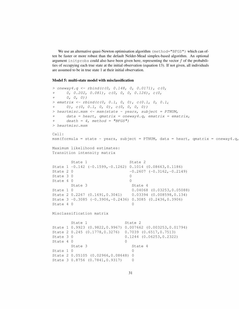
We use an alternative quasi-Newton optimisation algorithm (method="BFGS") which can of-ten be faster or more robust than the default Nelder-Mead simplex-based algorithm. An optionalargument initprobs could also have been given here, representing the vector f of the probabili-ties of occupying each true state at the initial observation (equation 13). If not given, all individualsare assumed to be in true state 1 at their initial observation.

Model 5: multi-state model with misclassification

> oneway4.q <- rbind(c(0, 0.148, 0, 0.0171), c(0,+ 0, 0.202, 0.081), c(0, 0, 0, 0.126), c(0,+ 0, 0, 0))> ematrix <- rbind(c(0, 0.1, 0, 0), c(0.1, 0, 0.1,+ 0), c(0, 0.1, 0, 0), c(0, 0, 0, 0))> heartmisc.msm <- msm(state ~ years, subject = PTNUM,+ data = heart, qmatrix = oneway4.q, ematrix = ematrix,+ death = 4, method = "BFGS")> heartmisc.msm

Call:msm(formula = state ~ years, subject = PTNUM, data = heart, qmatrix = oneway4.q, ematrix = ematrix, death = 4, method = "BFGS")


State 1 State 2State 1 -0.142 (-0.1599,-0.1262) 0.1014 (0.08663,0.1186)State 2 0 -0.2607 (-0.3162,-0.2149)State 3 0 0State 4 0 0


Misclassification matrix

State 1 State 2State 1 0.9923 (0.9822,0.9967) 0.007662 (0.003253,0.01794)State 2 0.245 (0.1778,0.3276) 0.7039 (0.6517,0.7513)State 3 0 0.1244 (0.06253,0.2322)State 4 0 0

State 3 State 4State 1 0 0State 2 0.05105 (0.02966,0.08648) 0State 3 0.8756 (0.7841,0.9317) 0

31

State 4 0 1 (1,1)

-2 * log-likelihood: 3952

Thus there is an estimated probability of about 0.01 that mild/moderate CAV will be diagnosederroneously, but a rather higher probability of 0.24 that underlying mild/moderate CAV will be diag-nosed as CAV-free. Between the two CAV states, the mild state will be misdiagnosed as severe witha probability of 0.05, and the severe state will be misdiagnosed as mild with a probability of 0.12.

The model also estimates the progression rates through underlying states. An average of 7 years isspent disease-free, an average of 3.8 years is spent with mild/moderate disease, and periods of severedisease last 3.2 years on average before death.

2.14 Effects of covariates on misclassification ratesWe can investigate how the probabilities of misclassification depend on covariates in a similar wayto the transition intensities, using a misccovariates argument to msm. For example, we nowinclude female sex as a covariate for the misclassification probabilities. This requires an extra fourinitial values for the linear effect for each of the logit-probabilities, which we set to zero.

Model 6: misclassification model with misclassification probabilities modelled on sex

> miscinits <- c(0.148, 0.0171, 0.202, 0.081, 0.126,+ 0.1, 0.1, 0.1, 0.1, 0, 0, 0, 0)

> heartmiscsex.msm <- msm(state ~ years, subject = PTNUM,+ data = heart, qmatrix = oneway4.q, ematrix = ematrix,+ death = 4, misccovariates = ~sex, method = "BFGS")

> heartmiscsex.msm

Call:msm(formula = state ~ years, subject = PTNUM, data = heart, qmatrix = oneway4.q, ematrix = ematrix, misccovariates = ~sex, death = 4, method = "BFGS")




32

Misclassification matrix

State 1 State 2State 1 0.9947 (0.9126,0.9997) 0.005319 (0.0002941,0.08859)State 2 0.2513 (0.1741,0.3483) 0.6971 (0.6367,0.7514)State 3 0 0.1462 (0.07781,0.2578)State 4 0 0

State 3 State 4State 1 0 0State 2 0.05156 (0.02974,0.08795) 0State 3 0.8538 (0.7615,0.9144) 0State 4 0 1 (1,1)

Logit-linear effects of sex

State 1 State 2State 1 0 -5.615 (-29.06,17.83)State 2 1.327 (-0.3563,3.011) 0State 3 0 1.936 (0.1946,3.678)State 4 0 0

State 3 State 4State 1 0 0State 2 -0.6299 (-2.744,1.484) 0State 3 0 0State 4 0 0


Considering the large confidence intervals for the estimates, we do not see any significant effect ofsex on the fitted misclassification probabilities, so that men are no more or less likely than women tohave an inaccurate angiography scan.

2.15 Extractor functionsAs well as the functions described in section 2.9 for extracting useful information from fitted models,there are a number of extractor functions specific to models with misclassification.

Misclassification matrix The function ematrix.msm gives the estimated misclassification prob-ability matrix at the given covariate values. For illustration, the fitted misclassification proba-bilities for men and women in model 6 are given by

> ematrix.msm(heartmiscsex.msm, covariates = list(sex = 0))

State 1 State 2State 1 0.9896 (0.9776,0.9952) 0.01039 (0.004753,0.02257)State 2 0.2225 (0.1546,0.3093) 0.7221 (0.6665,0.7716)State 3 0 0.1195 (0.05971,0.2247)

33

State 4 0 0State 3 State 4

State 1 0 0State 2 0.05539 (0.0316,0.09533) 0State 3 0.8805 (0.7907,0.935) 0State 4 0 1 (1,1)

> ematrix.msm(heartmiscsex.msm, covariates = list(sex = 1))

State 1 State 2State 1 1 (1.749e-06,1) 3.823e-05 (2.555e-15,1)State 2 0.519 (0.1673,0.8528) 0.4507 (0.2794,0.6345)State 3 0 0.4847 (0.1572,0.8259)State 4 0 0

State 3 State 4State 1 0 0State 2 0.03029 (0.004057,0.1932) 0State 3 0.5153 (0.316,0.7099) 0State 4 0 1 (1,1)

although these are not useful in this situation as there was no significant gender difference inangiography accuracy. The standard errors for the estimates for women are higher, since thereare only 87 women in this set of 622 patients.

Odds ratios for misclassification The function odds.msm gives the estimated odds ratios corre-sponding to each covariate effect on the misclassification probabilities.

> odds.msm(heartmiscsex.msm)

$sexOR L U

Obs State 1 | State 2 3.77019 7.00e-01 2.03e+01Obs State 2 | State 1 0.00364 2.40e-13 5.52e+07Obs State 2 | State 3 6.93300 1.21e+00 3.96e+01Obs State 3 | State 2 0.53263 6.43e-02 4.41e+00

underlining the lack of evidence for any gender difference in misclassification.

Observed and expected prevalences The function prevalence.msm is intended to assess thegoodness of fit of the hidden Markov model for the observed states to the data. Tables of ob-served prevalences of observed states are calculated as described in section 2.12, by assumingthat observed states are retained between observation times.

The expected numbers of individuals in each observed state are calculated similarly. Supposethe process begins at a common time for all individuals, and at this time, the probability ofoccupying true state r is fr. Then given n(t) individuals under observation at time t, the ex-pected number of individuals in true state r at time t is the rth element of the vector n(t)fP (t).Thus the expected number of individuals in observed state r is the rth element of the vectorn(t)fP (t)E, where E is the misclassification probability matrix.

34

The expected prevalences (not shown) for this example are similar to those forecasted by themodel without misclassification, with underestimates of the rates of death from 8 years on-wards. To improve this model’s long-term prediction ability, it is probably necessary to accountfor the natural increase in the hazard of death from any cause as people become older.

2.16 Recreating the path through underlying statesIn speech recognition and signal processing, decoding is the procedure of determining the underlyingstates that are most likely to have given rise to the observations. The most common method ofreconstructing the most likely state path is the Viterbi algorithm. Originally proposed by Viterbi [30],it is also described by Durbin et al. [20] and Macdonald and Zucchini [25] for discrete-time hiddenMarkov chains. For continuous-time models it proceeds as follows. Suppose that a hidden Markovmodel has been fitted and a Markov transition matrix P (t) and misclassification matrix E are known.Let vi(k) be the probability of the most probable path ending in state k at time ti.

1. Estimate vk(t1) using known or estimated initial-state occupation probabilities.

2. For i = 1 . . . N , calculate vl(ti) = el,Otimaxk vk(ti−1)Pkl(ti − ti−1). Let Ki(l) be the

maximising value of k.

3. At the final time point N , the most likely underlying state S∗N is the value of k which maximisesvk(TN ).

4. Retrace back through the time points, setting S∗i−1 = Ki(S∗i ).

The computations should be done in log space to prevent underflow. The msm package providesthe function viterbi.msm to implement this method. For example, the following is an extract froma result of calling viterbi.msm to determine the most likely underlying states for all patients. Theresults for patient 100103 are shown, who appeared to ‘recover’ to a less severe state of disease whilein state 3. We assume this is not biologically possible for the true states, so we expect that either theobservation of state 3 at time 4.98 was an erroneous observation of state 2, or their apparent state2 at time 5.94 was actually state 3. According to the expected path constructed using the Viterbialgorithm, it is the observation at time 5.94 which is most probably misclassified.

> vit <- viterbi.msm(heartmisc.msm)> vit[vit$subject == 100103, ]

subject time observed fitted567 100103 0.00 1 1568 100103 2.04 1 1569 100103 4.08 2 2570 100103 4.98 3 3571 100103 5.94 2 3572 100103 7.01 3 3573 100103 8.05 3 3574 100103 8.44 4 4

35

2.17 Fitting general hidden Markov models with msmThe msm package provides a framework for fitting continuous-time hidden Markov models withgeneral, continuous outcomes. As before, we use the msm function itself.

Specifying the hidden Markov model A hidden Markov model consists of two related compo-nents:

• the model for the evolution of the underlying Markov chain,

• the set of models for the observed data conditionally on each underlying state.

The model for the transitions between underlying states is specified as before, by supplying aqmatrix. The model for the outcomes is specified using the argument hmodel to msm. This is alist, with one element for each underlying state, in order. Each element of the list should be an objectreturned by a hidden Markov model constructor function. The HMM constructor functions providedwith msm are listed in Table 1. There is a separate constructor function for each class of outcomedistribution, such as uniform, normal or gamma.

Consider a three-state hidden Markov model, with a transition intensity matrix of

Q =

−q12 q12 00 −q23 q23

0 0 0

Suppose the outcome distribution for state 1 is Normal(µ1, σ

21), the distribution for state 2 is Normal(µ2, σ

22),

and state 3 is exactly observed. Observations of state 3 are given a label of -9 in the data. Here ourhmodel argument should be a list of objects returned by hmmNorm and hmmIdent constructorfunctions.

We must specify initial values for the parameters as the arguments to the constructor functions.For example, we take initial values of µ1 = 90, σ1 = 8, µ2 = 70, σ2 = 8. Initial values for q12 andq23 are 0.25 and 0.2. Finally suppose the observed data are in a variable called y, the measurementtimes are in time, and subject identifiers are in ptnum. The call to msm to estimate the parametersof this hidden Markov model would then be

msm ( y ~ time, subject=ptnum, data = example.df,qmatrix = rbind( c(0, 0.25, 0), c(0, 0, 0.2), c(0, 0, 0)),hmodel = list (hmmNorm(mean=90, sd=8), hmmNorm(mean=70, sd=8),

hmmIdent(-9)) )

Covariates on hidden Markov model parameters Most of the outcome distributions can be pa-rameterised by covariates, using a link-transformed linear model. For example, an observation yij

may have distribution f1 conditionally on underlying state 1. The link-transformed parameter θ1 is alinear function of the covariate vector xij at the same observation time.

yij |Sij ∼ f1(y|θ1, γ1)g(θ1) = α + βT xij

36

Function Distribution Parameters Location (link) Density for an observation xhmmCat Categorical prob,

basecatp, c0 p (logit) px, x = 1, . . . , n

hmmIdent Identity x x0 Ix=x0hmmUnif Uniform lower,

upperl, u 1/(u− l), u ≤ x ≤ l

hmmNorm Normal mean, sd µ, σ µ (identity) φ(x, µ, σ) = 1√2πσ2

exp(−(x− µ)2/(2σ2))

hmmLNorm Log-normal meanlog,sdlog

µ, σ µ (identity) 1

x√

2πσ2exp(−(log x− µ)2/(2σ2))

hmmExp Exponential rate λ λ (log) λe−λx, x > 0

hmmGamma Gamma shape,rate

n, λ λ (log) λn

Γ(n) xn−1 exp(−λx), x > 0, n > 0, λ > 0

hmmWeibull Weibull shape,scale

a, b b (log) ab ( x

b )a−1 exp (−( xb )a), x > 0

hmmPois Poisson rate λ λ (log) λx exp(−λ)/x!, x = 0, 1, 2, . . .

hmmBinom Binomial size, prob n, p p (logit)(

nx

)px(1− p)n−x

hmmNBinom Negative binomial disp, prob n, p p (logit) Γ(x + n)/(Γ(n)x!)pn(1− p)x

hmmTNorm Truncated normal mean, sd,lower,upper

µ, σ, l, u µ (identity) φ(x, µ, σ)/(Φ(u, µ, σ)− Φ(l, µ, σ)),where Φ(x, µ, σ) =

∫ x

−∞φ(u, µ, σ)du

hmmMETNorm Normal with trun-cation and measure-ment error

mean, sd,lower,upper,sderr,meanerr

µ0, σ0, l, u,σε, µε

µε (identity) (Φ(u, µ2, σ3)− Φ(l, µ2, σ3))/(Φ(u, µ0, σ0)− Φ(l, µ0, σ0))×φ(x, µ0 + µε, σ2),σ22 = σ2

0 + σ2ε ,

σ3 = σ0σε/σ2,µ2 = (x− µε)σ

20 + µ0σ2

εhmmMEUnif Uniform with mea-

surement errorlower,upper,sderr,meanerr

l, u, µε, σε µε (identity) (Φ(x, µε + l, σε)− Φ(x, µε + u, σε))/(u− l)

Table 1: Hidden Markov model distributions in msm.

37

Specifically, parameters named as the “Location” parameter in Table 1 can be modelled in terms ofcovariates, with the given link function.

The hcovariates argument to msm specifies the model for covariates on the hidden Markovoutcome distributions. This is a list of the same length as the number of underlying states, andthe same length as the hmodel list. Each element of the list is a formula, in standard R linearmodel notation, defining the covariates on the distribution for the corresponding state. If there are nocovariates for a certain hidden state, then insert a NULL in the corresponding place in the list. Forexample, in the three-state normal-outcome example above, suppose that the normal means on states1 and 2 are parameterised by a single covariate x.

µ1 = α1 + β1xij , µ2 = α2 + β2xij .

The equivalent call to msm would be

msm ( state ~ time, subject=ptnum, data = example.df,qmatrix = rbind( c(0, 0.25, 0), c(0, 0, 0.2), c(0, 0, 0)),hmodel = list (hmmNorm(mean=90, sd=8), hmmNorm(mean=70, sd=8),

hmmIdent(-9)),hcovariates = list ( ~ x, ~ x, NULL)).

Constraints on hidden Markov model parameters Sometimes it is realistic that parameters areshared between some of the state-specific outcome distributions. For example, the Normally-distributedoutcome in the previous example could have a common variance σ2

1 = σ22 = σ2 between states 1 and

2, but differing means. It would also be realistic for any covariates on the mean to have a commoneffect β1 = β2 = β on the state 1 and 2 outcome distributions.

The argument hconstraint to msm specifies which hidden Markov model parameters areconstrained to be equal. This is a named list. Each element is a vector of constraints on the namedhidden Markov model parameter. The vector has length equal to the number of times that class ofparameter appears in the whole model. As for the other constraint arguments such as qconstraint,identical values of this vector indicate parameters constrained to be equal.

For example consider the three-state hidden Markov model described above, with normally-distributed outcomes for states 1 and 2. To constrain the outcome variance to be equal for states1 and 2, and to also constrain the effect of x on the outcome mean to be equal for states 1 and 2,specify

hconstraint = list(sd = c(1,1), x=c(1,1))

FEV1 after lung transplants Now we give an example of fitting a hidden Markov model to a realdataset. The data on FEV1 measurements from lung transplant recipients, described in 1.6.4, areprovided with the msm package in a dataset called fev.

> data(fev)

We fit models Models 1 and 2, each with three states and common Q matrix.

> three.q <- rbind(c(0, exp(-6), exp(-9)), c(0,+ 0, exp(-6)), c(0, 0, 0))

38

The simpler Model 1 is specified as follows. Under this model the FEV1 outcome is Normal withunknown mean and variance, and the mean and variance are different between BOS state 1 and state2. hcovariates specifies that the mean of the Normal outcome depends linearly on acute events.Specifically, this covariate is an indicator for the occurrence of an acute event within 14 days of theobservation, denoted acute in the data. As an initial guess, we suppose the mean FEV1 is 100%baseline in state 1, and 54% baseline in state 2, with corresponding standard deviations 16 and 18, andFEV1 observations coinciding with acute events are on average 8% baseline lower. hconstraintspecifies that the acute event effect is equal between state 1 and state 2.

Days of death are coded as 999 in the fev outcome variable.

> hmodel1 <- list(hmmNorm(mean = 100, sd = 16),+ hmmNorm(mean = 54, sd = 18), hmmIdent(999))> fev1.msm <- msm(fev ~ days, subject = ptnum, data = fev,+ qmatrix = three.q, death = 3, hmodel = hmodel1,+ hcovariates = list(~acute, ~acute, NULL),+ hcovinits = list(-8, -8, NULL), hconstraint = list(acute = c(1,+ 1)), method = "BFGS")> fev1.msm

Call:msm(formula = fev ~ days, subject = ptnum, data = fev, qmatrix = three.q, hmodel = hmodel1, hcovariates = list(~acute, ~acute, NULL), hcovinits = list(-8, -8, NULL), hconstraint = list(acute = c(1, 1)), death = 3, method = "BFGS")


State 1State 1 -0.0007038 (-0.0008333,-0.0005945)State 2 0State 3 0

State 2State 1 0.0006275 (0.0005201,0.0007572)State 2 -0.0008011 (-0.001013,-0.0006337)State 3 0

State 3State 1 7.631e-05 (3.967e-05,0.0001468)State 2 0.0008011 (0.0006337,0.001013)State 3 0

Hidden Markov model, 3 statesInitial state occupancy probabilities: 1,0,0

State 1 - normal distributionParameters:

estimate l95 u95mean 98.0 97.34 98.67sd 16.2 15.78 16.60

39

acute -8.8 -9.95 -7.63

State 2 - normal distributionParameters:

estimate l95 u95mean 51.8 50.76 52.88sd 17.7 17.08 18.29acute -8.8 -9.95 -7.63

State 3 - identity distributionParameters:

estimate l95 u95which 999 NA NA


> sojourn.msm(fev1.msm)

estimates SE L UState 1 1421 122 1200 1682State 2 1248 149 987 1578

Printing the msm object fev1.msm shows estimates and confidence intervals for the transitionintensity matrix and the hidden Markov model parameters. The estimated within-state means of FEV1

are around 98% and 52% baseline respectively. From the estimated transition intensities, individualsspend around 1421 days (3.9 years) before getting BOS, after which they live for an average of 1248days (3.4 years). FEV1 is lower by an average of 8% baseline within 14 days of acute events.

Model 2, where the outcome distribution is a more complex two-level model, is specified asfollows. We use the distribution defined by equations 15–16. The hmmMETNorm constructor definesthe truncated normal outcome with an additional normal measurement error. The explicit probabilitydensity for this distribution is given in Table 1.

Our initial values are again 100 and 54 for the means of the within-state distribution of underlyingFEV1, and 16 and 18 for the standard errors. This time, underlying FEV1 is truncated normal. Thetruncation limits lower and upper are not estimated. We take an initial measurement error standarddeviation of sderr=8. The extra shift meanerr in the measurement error model is fixed to zeroand not estimated.

The hconstraint specifies that the measurement error variance σ2ε is equal between responses

in states 1 and 2, as is the effect of short-term acute events on the FEV1 response.

> hmodel2 <- list(hmmMETNorm(mean = 100, sd = 16,+ sderr = 8, lower = 80, upper = Inf, meanerr = 0),+ hmmMETNorm(mean = 54, sd = 18, sderr = 8,+ lower = 0, upper = 80, meanerr = 0), hmmIdent(999))> fev2.msm <- msm(fev ~ days, subject = ptnum, data = fev,+ qmatrix = three.q, death = 3, hmodel = hmodel2,+ hcovariates = list(~acute, ~acute, NULL),

40

+ hcovinits = list(-8, -8, NULL), hconstraint = list(sderr = c(1,+ 1), acute = c(1, 1)), method = "BFGS")> fev2.msm

Call:msm(formula = fev ~ days, subject = ptnum, data = fev, qmatrix = three.q, hmodel = hmodel2, hcovariates = list(~acute, ~acute, NULL), hcovinits = list(-8, -8, NULL), hconstraint = list(sderr = c(1, 1), acute = c(1, 1)), death = 3, method = "BFGS")


State 1State 1 -0.0007629 (-0.0008978,-0.0006483)State 2 0State 3 0

State 2State 1 0.0006912 (0.000578,0.0008266)State 2 -0.0007507 (-0.0009445,-0.0005967)State 3 0

State 3State 1 7.17e-05 (3.563e-05,0.0001443)State 2 0.0007507 (0.0005967,0.0009445)State 3 0

Hidden Markov model, 3 statesInitial state occupancy probabilities: 1,0,0

State 1 - metruncnorm distributionParameters:

estimate l95 u95mean 88.70 85.56 91.84sd 18.99 17.40 20.72lower 80.00 NA NAupper Inf NA NAsderr 8.88 8.42 9.38meanerr 0.00 NA NAacute -10.18 -11.24 -9.11

State 2 - metruncnorm distributionParameters:

estimate l95 u95mean 59.65 56.96 62.34sd 20.96 19.08 23.01lower 0.00 NA NAupper 80.00 NA NAsderr 8.88 8.42 9.38meanerr 0.00 NA NA

41

acute -10.18 -11.24 -9.11




> sojourn.msm(fev2.msm)

estimates SE L UState 1 1311 109 1114 1543State 2 1332 156 1059 1676

Under this model the standard deviation of FEV1 measurements caused by measurement error(more realistically, natural short-term fluctuation) is around 9% baseline. The estimated effect ofacute events on FEV1 and sojourn times in the BOS-free state and in BOS before death are similar toModel 1.

The following plot illustrates a trajectory of declining FEV1 from the first lung transplant recipientin this dataset. This is produced by the following R code. The Viterbi algorithm is used to locate themost likely point at which this individual moved from BOS state 1 to BOS state 2, according to thefitted Model 2. This is illustrated by the vertical dotted line. This is the point at which the individual’slung function started to remain consistently below 80% baseline FEV1.

> keep <- fev$ptnum == 1 & fev$fev < 999> plot(fev$days[keep], fev$fev[keep], type = "l",+ ylab = expression(paste("% baseline ", FEV[1])),+ xlab = "Days after transplant")> vit <- viterbi.msm(fev2.msm)[keep, ]> (max1 <- max(vit$time[vit$fitted == 1]))

[1] 2337

> (min2 <- min(vit$time[vit$fitted == 2]))

[1] 2367

> abline(v = mean(max1, min2), lty = 2)> text(max1 - 500, 50, "STATE 1")> text(min2 + 500, 50, "STATE 2")

42

500 1000 1500 2000 2500 3000 3500

5060

7080

9010

011

0

Days after transplant

% b

asel

ine

FE

V1

STATE 1 STATE 2

An alternative way of specifying a misclassification model This general framework for specify-ing hidden Markov models can also be used to specify multi-state models with misclassification. Amisclassification model is a hidden Markov model with a categorical outcome distribution. So in-stead of an ematrix argument to msm, we can use a hmodel argument with hmmCat constructorfunctions.

hmmCat takes at least one argument prob, a vector of probabilities of observing outcomes of1, 2, . . . , n respectively, where n is the length of prob. All outcome probabilities with an initialvalue of zero are assumed to be fixed at zero. prob is scaled if necessary to sum to one.

The model in section 2.13 specifies that an individual occupying underlying state 1 can be ob-served as states 2 (and 1), underlying state 2 can be observed as states 1, 2 or 3, and state 3 can beobserved as states 2 or 3, and underlying state 4 (death) cannot be misclassified. Initial values of 0.1are given for the 1-2, 2-1, 2-3 and 3-2 misclassification probabilities.

This is equivalent to the model below, specified using a hmodel argument to msm. The maximumlikelihood estimates should be the same as before (Model 5).

> oneway4.q <- rbind(c(0, 0.148, 0, 0.0171), c(0,+ 0, 0.202, 0.081), c(0, 0, 0, 0.126), c(0,+ 0, 0, 0))

43

> heartmisc.msm <- msm(state ~ years, subject = PTNUM,+ data = heart, hmodel = list(hmmCat(c(0.9,+ 0.1, 0, 0)), hmmCat(c(0.1, 0.8, 0.1, 0)),+ hmmCat(c(0, 0.1, 0.9, 0)), hmmIdent(4)),+ qmatrix = oneway4.q, death = 4, method = "BFGS")> heartmisc.msm

Call:msm(formula = state ~ years, subject = PTNUM, data = heart, qmatrix = oneway4.q, hmodel = list(hmmCat(c(0.9, 0.1, 0, 0)), hmmCat(c(0.1, 0.8, 0.1, 0)), hmmCat(c(0, 0.1, 0.9, 0)), hmmIdent(4)), death = 4, method = "BFGS")




Hidden Markov model, 4 statesInitial state occupancy probabilities: 1,0,0,0

State 1 - categorical distributionParameters:

estimate l95 u95P(1) 0.99234 NA NAP(2) 0.00766 0.00325 0.0179P(3) 0.00000 NA NAP(4) 0.00000 NA NA


estimate l95 u95P(1) 0.245 0.1778 0.3276P(2) 0.704 NA NAP(3) 0.051 0.0297 0.0865P(4) 0.000 NA NA


estimate l95 u95

44

P(1) 0.000 NA NAP(2) 0.124 0.0625 0.232P(3) 0.876 NA NAP(4) 0.000 NA NA




2.17.1 Defining a new hidden Markov model distribution

Suppose the hidden Markov model outcome distributions supplied with msm (Table 1) are insuffi-cient. We want to define our own univariate distribution, called hmmNewDist, taking two parame-ters location and scale. Download the source package, for example msm-0.5.tar.gz forversion 0.5, from CRAN and edit the files in there, as follows.

1. Add an element to .msm.HMODELPARS in the file R/constants.R, naming the parametersof the distribution. For example

newdist = c('location', 'scale')

2. Add a corresponding element to the C variable HMODELS in the file src/lik.c. This MUSTbe in the same position as in the .msm.HMODELPARS list. For example,

hmmfn HMODELS[] = {...,hmmNewDist

};.

3. The new distribution is allowed to have one parameter which can be modelled in terms of co-variates. Add the name of this parameter to the named vector .msm.LOCPARS in R/constants.R.For example newdist = ’location’. Specify newdist = NA if there is no such pa-rameter.

4. Supposed we have specified a parameter with a non-standard name, that is, one which doesn’talready appear in .msm.HMODELPARS. Standard names include, for example, ’mean’, ’sd’,’shape’ or ’scale’. Then we should add the allowed range of the parameter to .msm.PARRANGES.In this example, we add meanpars = c(-Inf, Inf) to .msm.PARRANGES. If the pa-rameter should always be fixed during a maximum likelihood estimation, then add its name to.msm.AUXPARS.

5. Add an R constructor function for the distribution to R/hmm-dists.R. For a simple univari-ate distribution, this is of the form

45

hmmNewDist <- function(location, scale){hmmDIST (label = "newdist",link = "identity",r = function(n) rnewdist(n, location, scale),match.call())

}

• The ’label’ must be the same as the name you supplied for the new element of.msm.HMODELPARS

• link is the link function for modelling the location parameter of the distribution asa function of covariates. This should be the quoted name of an R function. A loglink is ’log’ and a logit link is ’qlogis’. If using a new link function other than’identity’, ’log’, or ’qlogis’, you should add its name to the vector .msm.LINKFNSin R/constants.R, and add the name of the corresponding inverse link to .msm.INVLINK.You should also add the names of these functions to the C array LINKFNS in src/lik.c,and write the functions if they do not already exist.

• r is an R function, of the above format, returning a vector of n random values from thedistribution. You should write this if it doesn’t already exist.

6. Add the name of the new constructor function to the NAMESPACE in the top-level directoryof the source package.

7. Write a C function to compute the probability density of the distribution, and put this insrc/hmm.c, with a declaration in src/hmm.h. This must be of the form

double hmmNewDist(double x, double *pars)

where *pars is a vector of the parameters of the distribution, and the density is evaluated atx.

8. Update the documentation (man/hmm-dists.Rd and the distribution table in inst/doc/msm-manual.Rnw)if you like.

9. Recompile the package (see the “Writing R Extensions” manual)

Your new distribution will be available to use in the hmodel argument to msm, as, for example

hmodel = list (..., hmmNewDist(location = 0, scale = 1), ...)

If your distribution may be of interest to others, ask me nicely ([email protected])to include it in a future release.

46

3 msm reference guideThe R help page for msm gives details of all the allowed arguments and options to the msm function.To view this online in R, type:

> help(msm)

Similarly all the other functions in the package have help pages, which should always be con-sulted in case of doubt about how to call them. The web-browser based help interface may often beconvenient - type

> help.start()

and navigate to Packages . . . msm, which brings up a list of all the functions in the package withlinks to their documentation, and a link to this manual in PDF format.

A Changes in the msm packageVersion 0.5 is a major update to msm, introducing hidden Markov models with general responses.Much of the underlying R and C code was re-organised or re-written. Some syntax changes weremade to simplify the process of specifying models.

To convert code written for previous versions of msm to run in 0.5, the following changes willneed to be made.

• Replace the qmatrix of ones and zeroes with a qmatrix containing initial values for tran-sition intensities.

• Replace the ematrix of ones and zeroes with a ematrix containing initial values for mis-classification probabilities.

• Put any initial values for covariate effects in covinits or misccovinits arguments.These are set to zero if not specified.

• Remove the inits argument.

• Remove unnecessary misc = TRUE for misclassification models.

• Replace any fromto-style datasets with proper longitudinal datasets with one row per obser-vation time. fromto support has been withdrawn.

• covmatch has been abolished. If you were using covmatch=’next’, covariates will needto be matched with observations by moving covariates one row back in the data.

• crudeinits.msm now takes an formula state ∼ time instead of two arguments state,time

• simmulti.msm takes an argument covariates instead of beta, for consistency withmsm.

47

Saved model objects from previous versions will need to be generated again under 0.5 to workwith the post-processing functions from 0.5.

For a more detailed list of the changes introduced in Version 0.5, see the NEWS file in the top-leveldirectory of the installed package.

If you use msm in published work, please let me know, for my own interest! Or even if you justuse it and find it helpful, whatever your field of application.

48

References[1] D. R. Cox and H. D. Miller. The Theory of Stochastic Processes. Chapman and Hall, London,

1965.

[2] C. H. Jackson, L. D. Sharples, S. G. Thompson, S. W. Duffy, and E. Couto. Multistate Markovmodels for disease progression with classification error. Journal of the Royal Statistical Society,Series D - The Statistician, 52(2):193–209, July 2003.

[3] C. H. Jackson and L. D. Sharples. Hidden Markov models for the onset and progression ofbronchiolitis obliterans syndrome in lung transplant recipients. Statistics in Medicine, 21:113–128, 2002.

[4] L. D. Sharples. Use of the Gibbs sampler to estimate transition rates between grades of coronarydisease following cardiac transplantation. Statistics in Medicine, 12:1155–1169, 1993.

[5] J. H. Klotz and L. D. Sharples. Estimation for a Markov heart transplant model. The Statistician,43(3):431–436, 1994.

[6] R. Kay. A Markov model for analysing cancer markers and disease states in survival studies.Biometrics, 42:855–865, 1986.

[7] I. M. Longini, W. S. Clark, R. H. Byers, J. W. Ward, W. W. Darrow, G. F. Lemp, and H. W.Hethcote. Statistical analysis of the stages of HIV infection using a Markov model. Statistics inMedicine, 8:851–843, 1989.

[8] G. A. Satten and I. M. Longini. Markov chains with measurement error: Estimating the ‘true’course of a marker of the progression of human immunodeficiency virus disease. Applied Statis-tics - Journal of the Royal Statistical Society Series C, 45(3):275–295, 1996.

[9] C. Guihenneuc-Jouyaux, S. Richardson, and I. M. Longini. Modelling markers of disease pro-gression by a hidden Markov process: Application to characterising CD4 cell decline. Biomet-rics, 56:733–741, 2000.

[10] R. C. Gentleman, J. F. Lawless, J. C. Lindsey, and P. Yan. Multi-state Markov models foranalysing incomplete disease history data with illustrations for HIV disease. Statistics inMedicine, 13(3):805–821, 1994.

[11] G. Marshall and R. H. Jones. Multi-state Markov models and diabetic retinopathy. Statistics inMedicine, 14, 1995.

[12] P. K. Andersen. Multistate models in survival analysis: a study of nephropathy and mortality indiabetes. Statistics in Medicine, 7(6):661–670, 1988.

[13] S. W. Duffy and H. H. Chen. Estimation of mean sojourn time in breast cancer screeningusing a Markov chain model of entry to and exit from preclinical detectable phase. Statistics inMedicine, 14:1531–1543, 1995.

[14] H. H. Chen, S. W. Duffy, and L. Tabar. A Markov chain method to estimate the tumour progres-sion rate from preclinical to clinical phase, sensitivity and positive predictive value for mam-mography in breast cancer screening. The Statistician, 45(3):307–317, 1996.

49

[15] A. J. Kirby and D. J. Spiegelhalter. Statistical modelling for the precursors of cervical cancer.In Case Studies in Biometry. Wiley, New York, 1994.

[16] P. K. Andersen, L. S. Hansen, and N. Keiding. Assessing the influence of reversible diseaseindicators on survival. Statistics in Medicine, 10:1061–1067, 1991.

[17] J. Grüger, R. Kay, and M. Schumacher. The validity of inferences based on incomplete obser-vations in disease state models. Biometrics, 47:595–605, 1991.

[18] J.D. Kalbfleisch and J.F. Lawless. The analysis of panel data under a Markov assumption.Journal of the American Statistical Association, 80(392):863–871, 1985.

[19] B. H. Juang and L. R. Rabiner. Hidden Markov models for speech recognition. Technometrics,33:251–272, 1991.

[20] R. Durbin, S. Eddy, A. Krogh, and G. Mitchison. Biological Sequence Analysis: ProbabilisticModels of Proteins and Nucleic Acids. Cambridge University Press, 1998.

[21] L. E. Baum and T. Petrie. Statistical inference for probabilistic functions of finite state Markovchains. Annals of Mathematical Statistics, 37:1554–1563, 1966.

[22] L. E. Baum, T. Petrie, G. Soules, and N. Weiss. A maximisation technique occurring in the sta-tistical analysis of probabilistic functions of Markov chains. Annals of Mathematical Statistics,41:164–171, 1970.

[23] P. S. Albert. A mover-stayer model for longitudinal marker data. Biometrics, 55(4):1252–1257,1999.

[24] A. Bureau, J. P. Hughes, and S. C. Shiboski. An S-Plus implementation of hidden Markovmodels in continuous time. Journal of Computational and Graphical Statistics, 9:621–632,2000.

[25] I. L. Macdonald and W. Zucchini. Hidden Markov and Other Models for Discrete-Valued TimeSeries. Chapman and Hall, London, 1997.

[26] J. K. Lindsey. Models for Repeated Measurements. Oxford Statistical Science Series. OxfordUniversity Press, second edition, 1999.

[27] P. Guttorp. Stochastic Modeling of Scientific Data. Chapman and Hall, London, 1995.

[28] C. H. Jackson. Statistical models for the latent progression of chronic diseases using serialbiomarkers. PhD thesis, University of Cambridge, 2002.

[29] L.D. Sharples, C.H. Jackson, J. Parameshwar, J. Wallwork, and S.R. Large. Diagnostic accuracyof coronary angiography and risk factors for post-heart-transplant cardiac allograft vasculopa-thy. Transplantation, 76(4):679–682, 2003.

[30] J. Viterbi. Error bounds for convolutional codes and an asymptotically optimal decoding algo-rithm. IEEE Transactions on Information Theory, 13:260–269, 1967.

50

multi-state modelling with r: the msm package -...

Documents