multi-resolution modeling with dta existing deployments · 2016-02-25 · multi-resolution modeling...

Multi-Resolution Modeling with DTAExisting Deployments

A Information Sharing Workshop for Dynamic Traffic Assignment

Yi-Chang Chiu, Eric Pihl, Nick Renna

Sponsored by:Federal Highway Administration

Resource Center, Michigan DivisionMichigan Department of Transportation

Lansing, MichiganWednesday, August 11, 2010

8/16/2010 1

Who else are using DTA (Federal)?

• FHWA - Integrated Corridor Management

– 2 out of 3 pioneering sites (Minneapolis and Dallas)

• FHWA – Exploratory Advanced Research Program

– Integrating land-use, activity-based model and DTA

• FHWA – Real-Time Traffic Estimation and Prediction

– TrEPS – for real-time ITS based active traffic management


• TRB – Strategic Highway Research Program (SHRP2)– C04 - Improving Our Understanding of How Highway

Congestion and Pricing Affect Travel Demand– C05 - Understanding the Contribution of Operations,

Technology, and Design to Meeting Highway CapacityNeeds

– C10 - Partnership to Develop an Integrated, Advanced Travel Demand Model and a Fine-Grained, Time Sensitive Network

– L04 - Incorporating Reliability Performance Measures in Operations and Planning Modeling Tools

– R11 - Strategic Approaches at the Corridor and Network Level to Minimize Disruption from the Renewal Process


• EPA – Motor Vehicle Emission Simulators (MOVES)– “When fully implemented, MOVES will serve as the

replacement for MOBILE6 and NONROAD for all official analyses associated with regulatory development, compliance with statutory requirements, and national/regional inventory projections.”

– Official released Fall 2009

– Tighter integration with regional traffic simulation models

Who else are using DTA (States)?

• IH corridor improvement (North

Carolina)

• IH work zone planning (ELP, TX-2004)

• Evacuation operational Planning (Houston, TX, 2007, Baltimore, MD, 2005, Knoxville, TN, 2003)

• Florida turnpike system traffic and evacuation analysis (FDOT Turnpike)

• Downtown improvement (ELP, TX, 2004)

• ICM AMS modeling (Bay Area, CA, 2007)

Who else are using DTA (States)?• Military deployment transportation improvement in

Guam (PB, FHWA)

• Interstate highway corridor improvement (TTI, TxDOT,

ELPMPO, Kittleson, ADOT)

• Value pricing (ORNL, FHWA; SRF, Mn/DOT, TTI, TxDOT, UA,

CDOT/DRCOG)

• Evacuation operational planning (TTI, TxDOT, UA, ADOT;

LSU, LDOT; Noblis, FHWA; Univ. of Toronto, Cornell Univ. Jackson State Univ., MDOT, Univ. of Missouri, MDOT)

• Integrated Corridor Management modeling (CS, FHWA,

MAG, NCSU, NCDOT)

• Pilot studies (Portland Metro, DRCOG)

• Activity-based model integration (UA/CS, SHRP2 C10,

FHWA EARP)

• Work zone impact management (SHRP2 R11)

Compatibility with Existing Modeling Framework

• Trip-based framework

– Replace static assignment

– Sub-area analysis in micro traffic models

– Relative standard

Trip Generation

Model

Trip Distribution

Model

Mode Choice Model

Time of Day Model

Mesoscopic Dynamic

Traffic Assignment

Jurisdiction

Sub-Area

Model 1

Jurisdiction

Sub-Area

Model 2

Jurisdiction

Sub-Area

Model 3

Mic

rosc

op

ic o

r

Me

sosc

op

icM

eso

sco

pic

Ma

cro

sco

pic

Skims

Network

Performance

Measure

Strategic Modeling

Mission-Driven Modeling

Capability Expansion not Replacement

• Multi-Resolution Modeling - Synergize existing model capabilities– Dynamic view of entire system

– Rapid and consistent sub-area analysesMeso MicroMacro

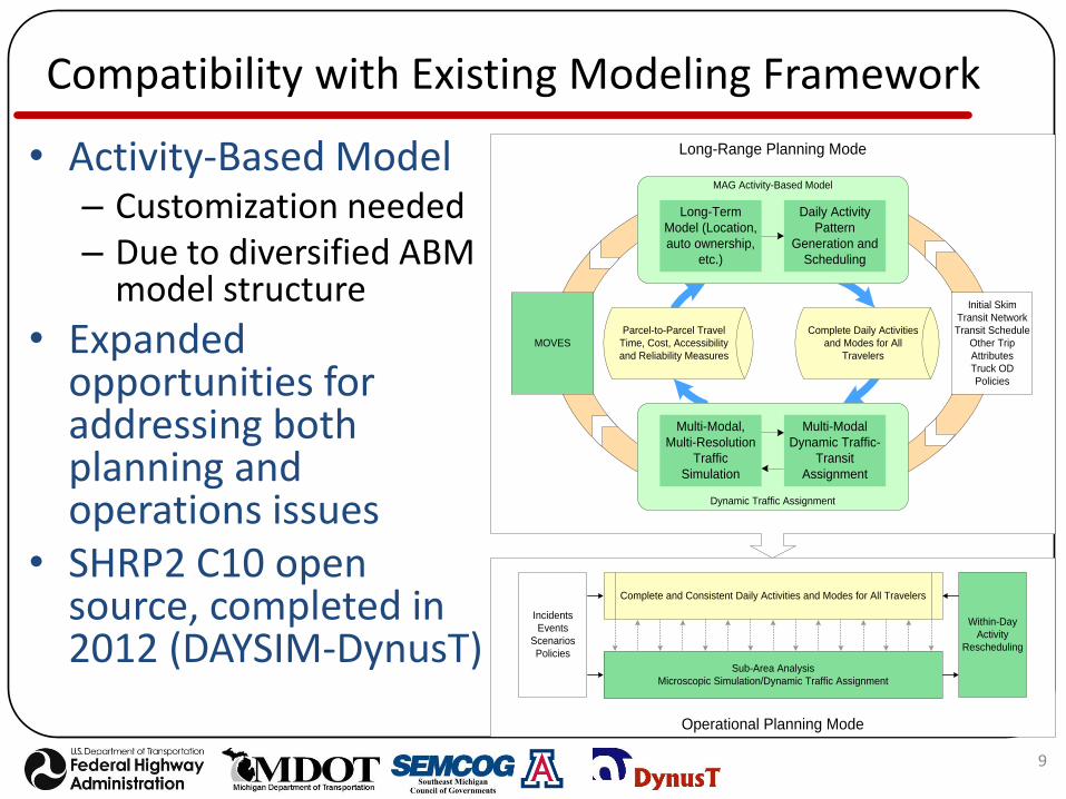
Compatibility with Existing Modeling Framework

• Activity-Based Model– Customization needed– Due to diversified ABM

model structure

• Expanded opportunities for addressing both planning and operations issues

• SHRP2 C10 open source, completed in 2012 (DAYSIM-DynusT)

9

Long-Range Planning Mode

Operational Planning Mode

Complete Daily Activities

and Modes for All

Travelers

Parcel-to-Parcel Travel

Time, Cost, Accessibility

and Reliability Measures

Initial Skim

Transit Network

Transit Schedule

Other Trip

Attributes

Truck OD

Policies

MOVES

Dynamic Traffic Assignment

Multi-Modal,

Multi-Resolution

Traffic

Simulation

Multi-Modal

Dynamic Traffic-

Transit

Assignment

MAG Activity-Based Model

Long-Term

Model (Location,

auto ownership,

etc.)

Daily Activity

Pattern

Generation and

Scheduling

Complete and Consistent Daily Activities and Modes for All Travelers

Sub-Area Analysis

Microscopic Simulation/Dynamic Traffic Assignment

Incidents

Events

Scenarios

Policies

Within-Day

Activity

Rescheduling

UrbanSim-OpenAMOS-MALTA/DynusT

• Evolutionary modeling, completed in 2011

8/16/2010 10

Future Year n

Base Year

Base Year Bootstrapping

Initial OD Trip

Tables

Dynamic Traffic

Assignment and

Simulation

Calibration Procedure

Observed Link

Traffic Data

Calibration

Converge?

OD Trip Times

N

Y

Dynamic Traffic

Assignment and

Simulation

Activity Travel Simulation

Assignment

Converged?OD Trip Times

N

Y

Dynamic Traffic

Assignment and

Simulation

Carry Over Delta


Assignment


N

Y

Land Use Model

Future Year n+1

Dynamic Traffic

Assignment and

Simulation

Carry Over Delta


Assignment


N

Y

Land Use Model

What is Multi-Resolution Modeling (MRM)?

• Integrating macro, meso and micro traffic analysis tools with different levels of resolution and capabilities for the purpose of achieving a specific goal

– Analyze network at both the system-wide and localized levels simultaneously

Dynamic Static

0.1-1 second 5-10 seconds

Intersections Micro Sim

Corridor Micro Sim DTA

Regional DTA TDM

• Addresses issues that may fall beyond the reach of both:

– Macroscopic models: large scale but static

– Microscopic models: dynamic but small-scale

– DTA: dynamic and large-scale

• The scenarios of interest may result in shifts of network or corridor-wide traffic flow patterns

– Significant change to roadway configuration

– Certain corridor management strategies

What is Multi-Resolution Modeling (MRM)?

• Many commercial packages allow us to perform microscopic analysis by extracting sub-area directly from TDM, why do we need DTA as the “middle man?”

• To answer this, let’s look at the following question:

13

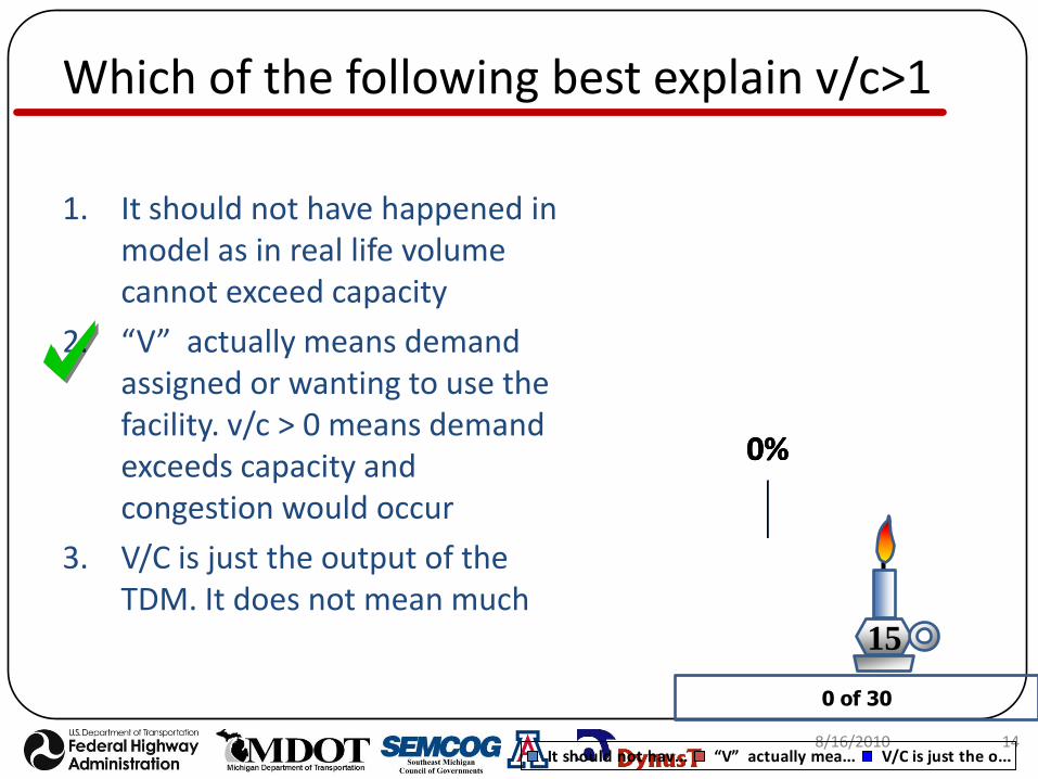
Which of the following best explain v/c>1

8/16/2010 14

0%0%0%

It should not hav... “V” actually mea... V/C is just the o...

1. It should not have happened in model as in real life volume cannot exceed capacity

2. “V” actually means demand assigned or wanting to use the facility. v/c > 0 means demand exceeds capacity and congestion would occur

3. V/C is just the output of the TDM. It does not mean much

15

0 of 30

Issue with Macro-Micro Integration

• OD flow arriving at boundary of sub-area is not constrained by roadway capacity outside the sub-area

• Consequences

– Too much demand, sub-area over flooded

– Hand-tweaking as calibration in baseline case

– Min prediction power for future year cases

8/16/2010 15

Meso MicroMacro

Macro-Meso-Micro

• Bridge macro and micro for a wide range of applications

Actual System Dynamics

DTA Describes System Structural Pattern

Micro Model Describes Finer Dynamic Details

Static Model Describes Overall Average

Peak PeriodTime

Co

nge

stio

n

Capability Expansion not Replacement

• Multi-Resolution Modeling - Synergize existing model capabilities– Dynamic view of entire system

– Rapid and consistent sub-area analysesMeso MicroMacro

Why is MRM Important?

• Macro, meso and micro models are not mutually exclusive

• They are complimentary to one another and can accomplish optimal modeling capabilities

• Retain the best characteristics of each model

– Incorporate multiple trip purposes

– Realistic representation of regional traffic in baseline and future years

– Provide realistic inputs to micro models

– A wide range of visual representation of model outputs

A Recent MRM RFP (DVRPC)

• See RFQ

208/16/2010

Network Conversion

Links

Nodes

Zones

TDM DTA model

• Convert the GIS layer of the travel demand model to mesoscopic format

• Disaggregate 24-hour matrix based upon car & truck– Home to work

– Work to home

– Home to private

– Private to home

– Thru

– External local

– Non-home based external local

• Multiply each matrix by corresponding hourly factor

Network Conversion

Network Conversion

H-W W-H H-P P-H THRU EXLO PEXLO

Multiply each matrix by hourly factor

Summation of matrices gives you directional 1-hour matrix

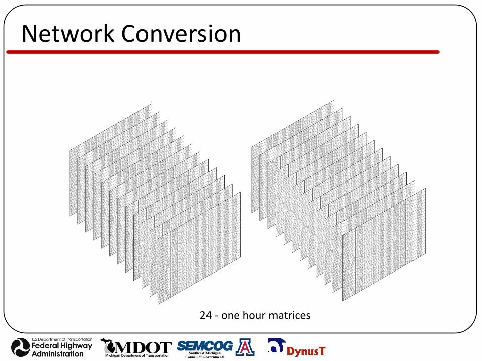
Network Conversion

24 - one hour matrices

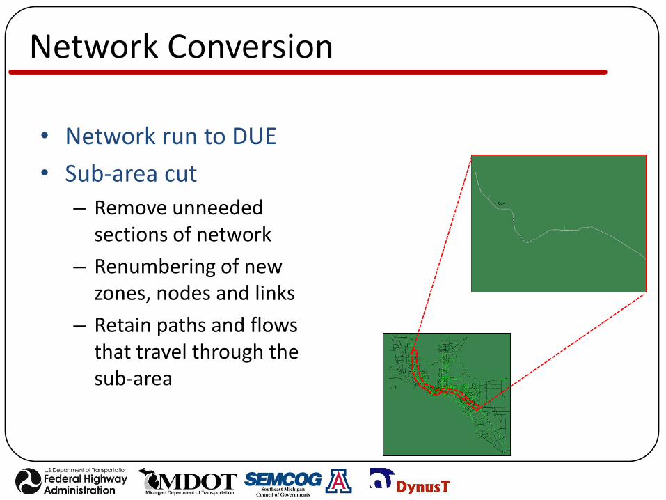
Network Conversion

• Network run to DUE

• Sub-area cut

– Remove unneeded sections of network

– Renumbering of new zones, nodes and links

– Retain paths and flows that travel through the sub-area

Network Conversion

• Meso-Micro Converter– Developed by researchers

from TTI and UA

– Converts roadway network to Macro network

– Retains network geometry

– Converts all time-dependent paths and flows

– Creates separate transportation systems (car, truck)

Network Conversion

• Microscopic model– Calibrate Micro model to

reflect realistic roadway conditions

– Perform detailed “fine-grained” analyses• Speed profile for individual

lanes

• Lane-changing behaviors

• Vehicle interactions at merge areas

– Create 3-D graphics for presentations

• Traffic flow model– Traffic simulation in

DynusT is based upon the Anisotropic Mesoscopic Simulation (AMS) model

– Moves vehicle based upon speed-density (v-k) relationship

– v-k relationship is derived from Greenshields equation

Calibration

Speed (mph)

De

nsi

ty (v

eh

/mi)

◆ Observed v■ Calibrated v

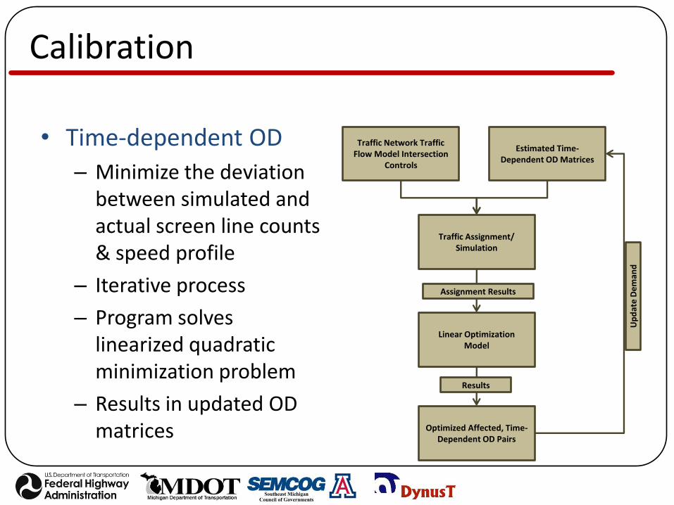
• Time-dependent OD

– Minimize the deviation between simulated and actual screen line counts & speed profile

– Iterative process

– Program solves linearized quadratic minimization problem

– Results in updated OD matrices

Calibration

Traffic Network Traffic Flow Model Intersection

Controls

Estimated Time-Dependent OD Matrices

Traffic Assignment/Simulation

Linear OptimizationModel

Optimized Affected, Time-Dependent OD Pairs

Results

Up

dat

e D

em

and

Assignment Results

• Network– Lane configuration

– Geometric design

• Paths and flows– Verify same origin/destination paths

– Verify number of vehicles generated

• Speed profile– Perform field data collection to determine speed and

vehicle counts

– Obtain v-k curve from simulation output

– Calibrate models with field data

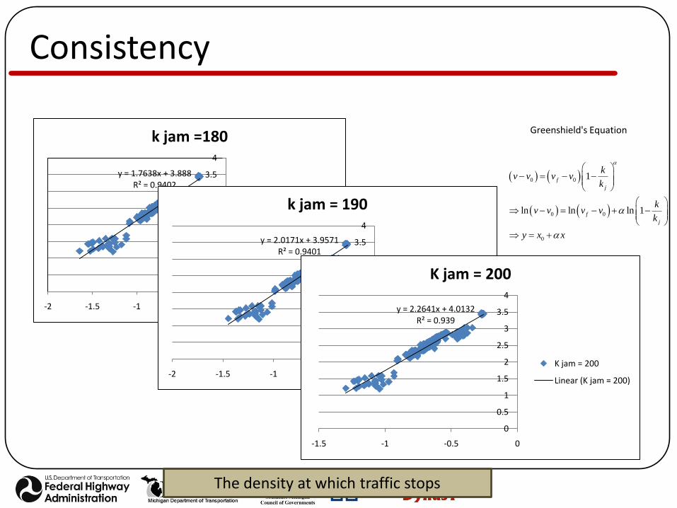
Consistency

Consistency

y = 1.7638x + 3.888R² = 0.9402

0

0.5

1

1.5

2

2.5

3

3.5

4

-2 -1.5 -1 -0.5 0

k jam =180

k jam =180

Linear (k jam =180)y = 2.0171x + 3.9571R² = 0.9401

0

0.5

1

1.5

2

2.5

3

3.5

4

-2 -1.5 -1 -0.5 0

k jam = 190

k jam = 190

Linear (k jam = 190)y = 2.2641x + 4.0132R² = 0.939

0

0.5

1

1.5

2

2.5

3

3.5

4

-1.5 -1 -0.5 0

K jam = 200

K jam = 200

Linear (K jam = 200)

The density at which traffic stops

0 0

0 0

0

1

ln ln ln 1

f

j

f

j

kv v v v

k

kv v v v

k

y x x

Greenshield's Equation

Consistency

Speed profile calibrated with field data

• Analyze the effectiveness of restricting trucks from left-most fast lane on freeway

• 22-mile corridor of I-10 in El Paso, TX

• Analyze a.m. peak, p.m. peak, & mid-day

• Determine benefits– Speed on left-most lane

– Acceleration/Deceleration patterns

– Vehicle interactions at merge areas

– Does grade play a significant role on truck speeds?

• How should we model this?

Case Study 1 – Truck Restricted Lanes (TTI)


• DTA model estimates region-wide truck and car trajectories (time-dependent paths and flows)

• Micro model gives detailed I-10 truck lane operations with truck trajectories


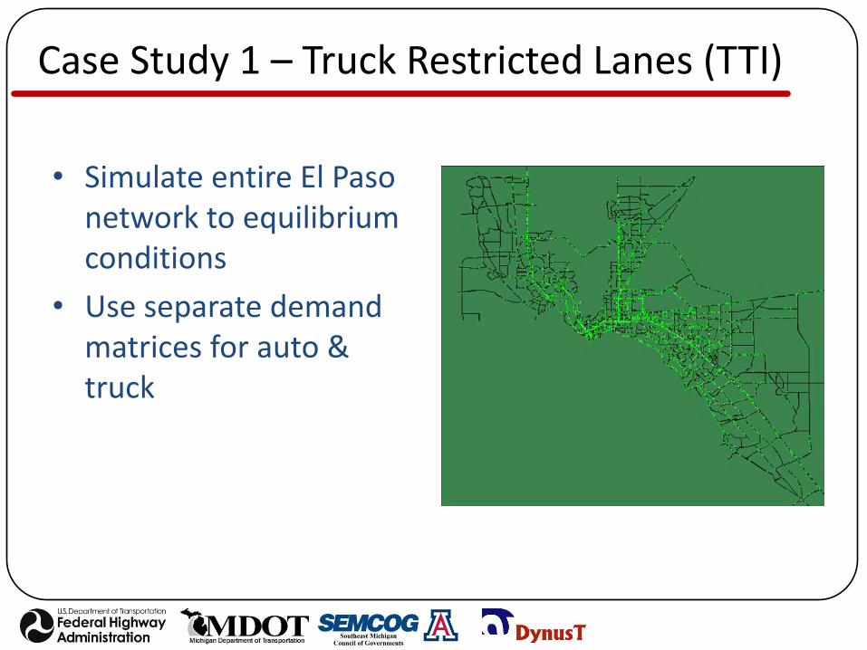
• Simulate entire El Paso network to equilibrium conditions

• Use separate demand matrices for auto & truck


• Sub-area cut of corridor was extracted

• Conversion tool was used to translate the roadway network, paths & flows to macro model

• Using macro models export capability, a microscopic simulation model was imported to microscopic format


DTA model

Micromodel

Macromodel

Sub-Area Conversion tool


• If modifications in the micro model change driver behavior (alters routes), changes must be reflected in DTA model and conversion process begins again.

• If no additional changes are needed, micro model development begins


106 Origin/Destination links - 1895 Routes created


GPS unit was used to input freeway grading information


Data provided by TxDOT Automatic Traffic Recorder Stations


56575859606162636465

0 3600 7200 10800 14400

Spe

ed

(mp

h)

Time (sec)

I-10 EB @ Sunland Park(7-11 am)

Base Restricted

-1.5

-1

-0.5

0

0.5

1

1.5

0 3600 7200 10800 14400

Acc

ele

rati

on

(ft

/s2

)

Time (sec)

I -10 EB @ Sunland Park(7-11 am)

Base Restricted

Speed Accel/Decel

Speed profile calibrated with field data

• Results showed that restricting trucks from left-most fast lane had slight improvement on speeds.

• Identified section of freeway where restrictions had adverse affect on freeway speeds

Case Study 1

0

20

40

60

80

0 3600 7200 10800 14400

Sp

ee

d (

mp

h)

Time (sec)

I-10 WB @ PaisanoLeft Lane (3-7 pm)

Base Restricted

0

20

40

60

80

0 3600 7200 10800 14400

Sp

ee

d (

mp

h)

Time (sec)

I-10 WB @ PaisanoRight Lane (3-7 pm)

Base Restricted

Speed – Left vs. Right Lane

• Texas Department of Transportation looking at alleviating congestion at diamond interchange and surrounding arterials in El Paso, TX.

• Propose 7 different design alternatives for direct connects

• Two sets of designs are identical except for direct connect lane access

• Corridor has heavy truck usage

Case Study 2

• TxDOT wants to know which alternative is most viable option?

• How does weaving at merge areas affect traffic on I-10?

• How dose improved LOS due to new interchange attract traffic to I-10 in the future?

• Analyze both the localized traffic impact and regional traffic redistribution

• Which model should we use?– Travel demand model?– DTA model?– Microscopic model?

Case Study 2 – Freeway Improvements (TTI)

• DTA model was able to show shifts in traffic based upon each design alternative.

– Queuing on arterials and frontage roads

– Speed fluctuations during peak hours

• Micro model was able to identify “hot-spot” areas where direct connects merge

• Micro model was used to determine whether or not grade played a major role on trucks entering freeway.


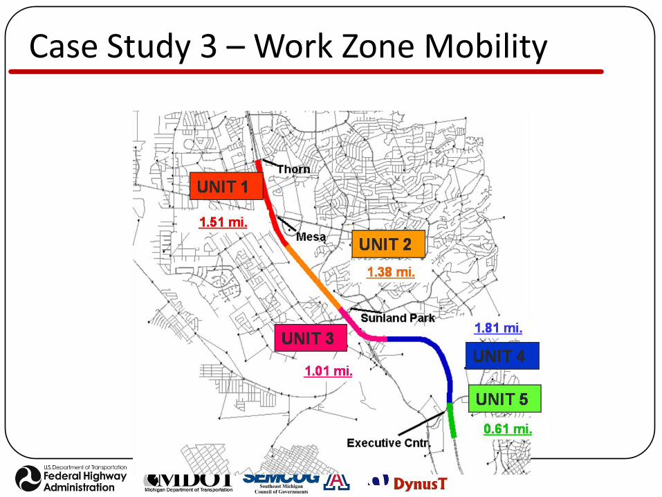
Case Study 3 – Work Zone Mobility

• Construction sequencing for addition of freeway lane

– TxDOT wants to widen section of I-10 in western portion of El Paso

– Construction divided into 5 section areas

– Determine optimal construction sequencing for TCP with moveable barriers


Determine optimal traffic flow in work zone during peak/non-peak hours using movable barriers

Varies

Varies

Varies

UNIT 3, ALTERNATE PHASE A, TYPICAL SECTION-OFF PEAK EASTBOUND

UNIT 3, ALTERNATE PHASE A, NIGHT AND WEEKENDS

Construction Joint 78'



UNIT 3, ALTERNATE PHASE A, TYPICAL SECTION-OFF PEAK WESTBOUND

EXPANDED WORK AREA 89 FEET

5 LANES @ 11 FEET

5 LANES @ 11 FEET

4 LANES @ 11 FEET

NORMAL WORK AREA 78 FEET


EastboundWestbound

Varies

Varies

Varies








5 LANES @ 11 FEET

5 LANES @ 11 FEET

4 LANES @ 11 FEET



Varies

Varies

Varies








5 LANES @ 11 FEET

5 LANES @ 11 FEET

4 LANES @ 11 FEET



Night Time

Westbound (PM) Peak hour

Eastbound (AM) Peak hour

Work Zone

Work Zone

Work Zone

Work Zone

UNIT 3

1.01 mi.


• DTA was able to evaluate effectiveness of TCPs

• Identify optimal construction sequencing of phases.

• Identify hotspots during peak and off-peak periods

• Evaluate possible mitigation strategies to help reduce congestion.


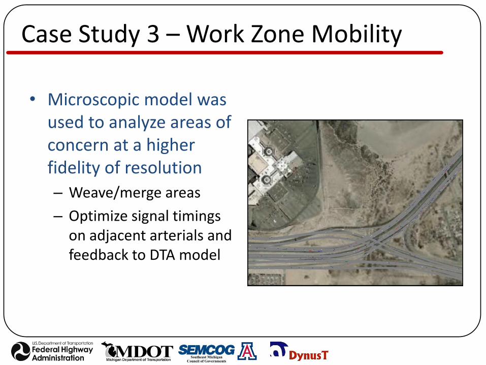
• Microscopic model was used to analyze areas of concern at a higher fidelity of resolution

– Weave/merge areas

– Optimize signal timings on adjacent arterials and feedback to DTA model

Case Study 4 - I-70 Zipper Lane Operational Planning

• 15-mile zipper Lane for I-70 EB during Sunday PM in ski season

• $20M capital, $9M O&M

555/10/2010

MRM Modeling Process

• Planning decisions– Fatal flaw of MBS– Tolling traffic and revenue forecast

• Operational Decisions– Queue length (WB)– East and West terminal configuration– Interchange re-design

• Model initial setup– Existing I-70 corridor network from a prior study (PEIS)

• Model calibration and validation– Traffic data from CDOT – Trip origins and destinations

565/10/2010

Model Initial Setup

1. Planning model

2. DTA model conversion

3. Subarea model

575/10/2010

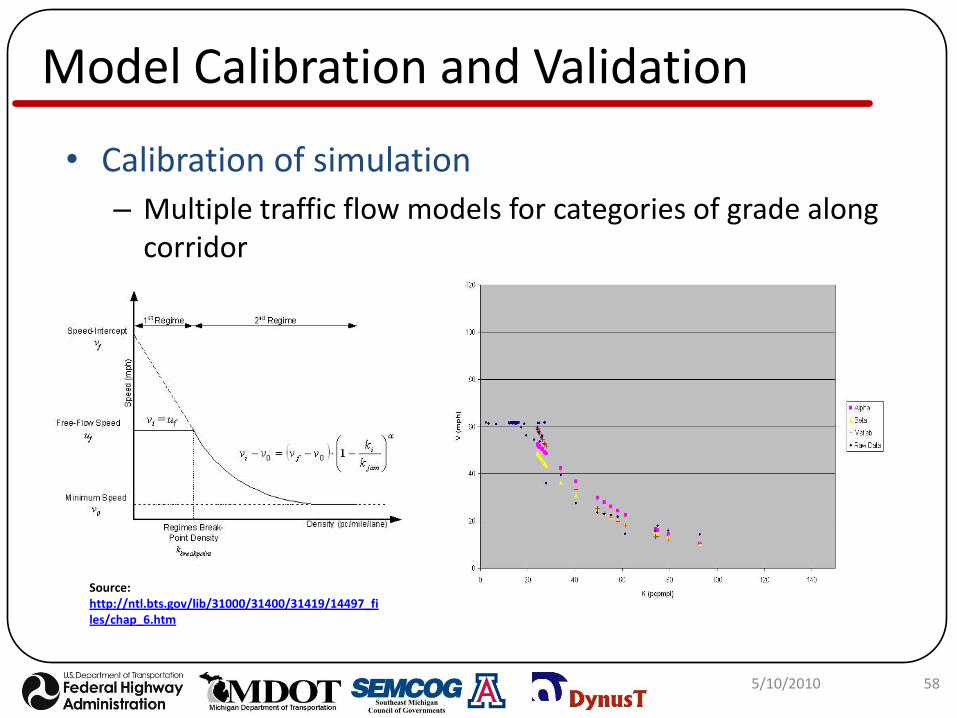
Model Calibration and Validation

• Calibration of simulation

– Multiple traffic flow models for categories of grade along corridor

Source: http://ntl.bts.gov/lib/31000/31400/31419/14497_files/chap_6.htm

585/10/2010

http://ntl.bts.gov/lib/31000/31400/31419/14497_files/chap_6.htm

http://ntl.bts.gov/lib/31000/31400/31419/14497_files/chap_6.htm


59

Total Link Counts

Speed Profile

Two-Stage Dynamic Calibration Framework

Stage 1OD Trips

Calibration

Discretize time horizon

Stage 2Departure Profile

calibration

Calibration time interval

5/10/2010


• OD calibration

– Match total traffic counts within time period at different locations along corridor

605/10/2010

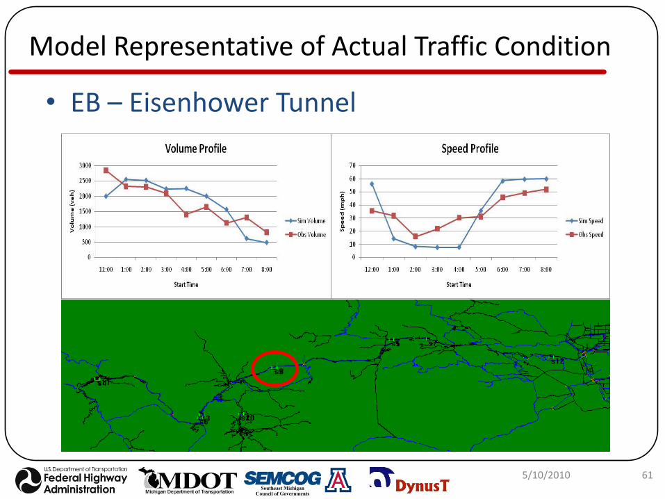
Model Representative of Actual Traffic Condition

• EB – Eisenhower Tunnel

615/10/2010

Scenario 1: Baseline (Existing Conditions)Direction: EB Main Lanes

625/10/2010

Scenario 2: Truck Allowed in EB Zipper Lane (No Toll)Direction: WB Single Main Lane

635/10/2010

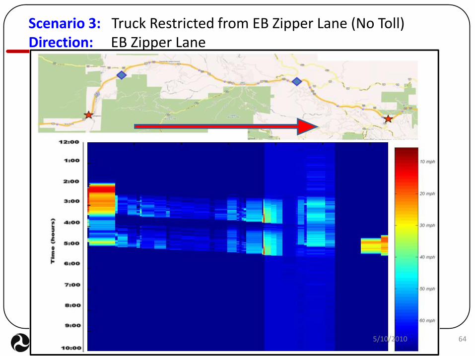
Scenario 3: Truck Restricted from EB Zipper Lane (No Toll)Direction: EB Zipper Lane

645/10/2010

Analysis Scenarios/Strategies

• Scenarios presented

1. Baseline (existing conditions)

2. Truck Allowed in EB Zipper Lane – No Toll

3. Truck Restricted from EB Zipper Lane – No Toll

4. Truck Restricted from EB Zipper Lane – Congestion Responsive Toll on Zipper Lane

5. Truck Restricted from EB Zipper Lane – Congestion Responsive Toll on Zipper Lane & WB Truck Diverted

655/10/2010

Questions?

5/10/2010 66

multi-resolution modeling with dta existing deployments · 2016-02-25 · multi-resolution modeling...

Documents