multi-objective optimization of hospital inpatient bed
TRANSCRIPT

Rochester Institute of Technology Rochester Institute of Technology
RIT Scholar Works RIT Scholar Works
Theses
8-8-2017
Multi-objective Optimization of Hospital Inpatient Bed Assignment Multi-objective Optimization of Hospital Inpatient Bed Assignment
Brenden Hoff [email protected]
Follow this and additional works at: https://scholarworks.rit.edu/theses
Recommended Citation Recommended Citation Hoff, Brenden, "Multi-objective Optimization of Hospital Inpatient Bed Assignment" (2017). Thesis. Rochester Institute of Technology. Accessed from
This Thesis is brought to you for free and open access by RIT Scholar Works. It has been accepted for inclusion in Theses by an authorized administrator of RIT Scholar Works. For more information, please contact [email protected].

i
Multi-objective Optimization of Hospital
Inpatient Bed Assignment
by
Brenden Hoff
A Thesis submitted in partial fulfillment of the
requirements for the degree of
Master of Science in Industrial and Systems Engineering
Department of Industrial and Systems Engineering
Kate Gleason College of Engineering
Rochester Institute of Technology
Rochester, NY
August 8, 2017

ii
DEPARTMENT OF INDUSTRIAL AND SYSTEMS ENGINEERING
KATE GLEASON COLLEGE OF ENGINEERING
ROCHESTER INSTITUTE OF TECHNOLOGY
ROCHESTER, NEW YORK
CERTIFICATE OF APPROVAL
MASTER OF SCIENCE DEGREE THESIS
The Master of Science Degree Thesis of Brenden Hoff
has been examined and approved by the
thesis committee as satisfactory for the
thesis requirement for the
Master of Science degree
Approved by:
Dr. Rubén Proaño, Thesis Advisor
Dr. Marcos Esterman, Committee Member

iii
Committee Approval:
Thesis: Multi-Objective Optimization of Hospital Inpatient Bed Assignment
Author: Brenden Hoff
Dr. Rubén A. Proaño Date
Thesis Advisor
Associate Professor, Rochester Institute of Technology, Industrial & Systems Engineering
Dr. Marcos Esterman Date
Committee Member
Associate Professor, Rochester Institute of Technology, Industrial & Systems Engineering

iv
Abstract
Choosing which bed to assign an admitted patient to in a hospital is a complex problem. There
are numerous factors to consider including the patient’s gender and isolation requirements,
current bed availability, and unit configurations. This problem must be solved each time a new
patient seeks admission resulting in rearrangement of already admitted patients. Each movement
of an already admitted patient increases the workload for hospital staff and also increases the risk
of nosocomial infections for the patient. In order to alleviate these problems we propose
optimizing the patient admission process through a multi-objective model which first maximizes
the overall criticality of patients admitted, then minimizes movements of previously admitted
patients while creating space for incoming patients. Using this model we perform three sets of
experiments. The first experiments seek to determine the ideal number of private and semi-
private rooms in a multi-occupancy unit with a fixed number of total rooms. This results in a tool
to enable the unit to manage the tradeoffs between moving previously admitted patients and bed
utilization. The second experiments seek to determine the ideal timeframe over which to batch
patient admissions. These results suggest more frequent admissions have minimal impact on
inpatient rearrangement. The third experiments seek to determine the potential benefit of using a
centralized admitting entity and finds managing bed assignment from a central perspective far
out performs individual units managing their bed assignments.

v
Contents
1. Introduction ............................................................................................................................................... 1
2. Problem Statement .................................................................................................................................... 4
3. Literature Review ...................................................................................................................................... 6
3.1 Bed Allocation .................................................................................................................................... 6
3.2 Bed Assignment .................................................................................................................................. 6
3.3 Bed Assignment with Unique Isolation Conditions .......................................................................... 10
3.4 Bed Pooling ....................................................................................................................................... 12
3.5 Bed Configuration within Units ........................................................................................................ 12
3.6 Need for a New Bed Assignment Model .......................................................................................... 13
4. Methodology Overview .......................................................................................................................... 14
4.1 Bed Assignment IP Model ................................................................................................................ 15
Sets ...................................................................................................................................................... 16
Parameters ........................................................................................................................................... 16
Variables ............................................................................................................................................. 16
Stage 1 ................................................................................................................................................. 18
Stage 2 ................................................................................................................................................. 19
4.2 Model Explanation ............................................................................................................................ 20
4.3 Experiments Overview ...................................................................................................................... 21
4.4 Assumptions ...................................................................................................................................... 23
5. Experiments and Results ......................................................................................................................... 24
5.1 Experiment A: Unit Demand ............................................................................................................ 24
Setup ................................................................................................................................................... 24
Results for Experiment A: Unit Demand ............................................................................................ 25
5.2 Experiment B: Batching .................................................................................................................... 30
Setup ................................................................................................................................................... 30
Results for Experiment B: Batching ................................................................................................... 31
5.3 Experiment C: Centralized Admission ............................................................................................. 37
Setup ................................................................................................................................................... 37
Results for Experiment C: Centralized Admission ............................................................................. 38
6. Discussion ............................................................................................................................................... 42

vi
6.1 Unit Demand ..................................................................................................................................... 42
6.2 Batching ............................................................................................................................................ 43
6.3 Centralized Admissions .................................................................................................................... 44
7. Future Work ............................................................................................................................................ 45
8. References ............................................................................................................................................... 46

1
1. Introduction
Healthcare Associated Infections (HAIs) or nosocomial infections have a major impact on
healthcare systems worldwide, affecting both patients and healthcare providers. HAIs are
infections that a patient acquires while in a healthcare setting which aggravate the conditions
they were originally hospitalized for [1]. The World Health Organization (WHO) Patient Safety
Unit is committed to raising awareness of HAIs and reducing their occurrence through process
improvements [2]. Their HAI fact sheet states that this problem spans both developed and
developing countries, affecting anywhere from 7-10% of hospitalized patients, with a larger
impact on patients admitted to intensive care units [3]. In the United States, both the Centers for
Disease Control and Prevention (CDC) and the Department of Health and Human Services
(HHS) have made it a public health priority to look for means to prevent and mitigate the
occurrence of HAIs [1]. As of 2014 the CDC lists 18 different infectious diseases and organisms
of concern in health care settings, including: influenza, norovirus, methicillin-resistant
Staphylococcus aureus (MRSA), and Clostridium difficle [4]. Often these infections occur as a
result of central-line catheterizations, urinary catheter placement, surgical site infection, or
ventilator usage [5].
Data compiled from 2011 by the CDC estimated that over 700,000 patients acquired an infection
during their stay in the hospital, and approximately 75,000 of those patients died during the
course of their hospitalization [6]. According to the National Institute for Health (NIH), one in
twenty inpatients at any time experience some form of a HAI [1]. Similarly, HHS estimates that
one in twenty-five inpatients at any given time is dealing with an infection they acquired while in
the hospital [7].
HAIs aggravate the conditions that patients were originally hospitalized for, contributing to tens
of thousands of patient deaths per year [1]. They also, at a minimum, can result in longer lengths
of stays and subsequent additional expenses. In 2013, Waknine [8] estimated that more than $9.8
billion is spent each year in the United States to treat HAIs, with some infections adding more
than $40,000 to the patient’s hospital bill.
The incidence of HAIs can also impact hospitals financially as well as affect patient satisfaction.
Hospitals extensively track their patient satisfaction and HAI rates, publishing these data to get a
promotional edge over neighboring hospitals. The 2010 Affordable Care Act (ACA) made

2
changes to Medicare reimbursement incorporating the hospital’s HCAHPS (patient satisfaction)
scores in the reimbursement formula used for paying providers for their services [9]. In addition
to patient satisfaction affecting reimbursement levels, hospitals can be forced to assume the cost
of dealing with HAIs. For example, Medicare reimbursement changes have reduced or
completely eliminated reimbursement to hospitals for treatment of certain HAIs [10, 11]. The
ACA also penalizes reimbursement rates for hospitals with the top 25% HAI rates [12]. These
costs add up to billions of dollars across the entire health care system each year [8]. Hospitals
can achieve substantial savings and better patient care by effectively controlling HAIs. Those
savings can then be used to implement programs to better test and treat patients, leading to
overall better patient outcomes.
The focus on HAIs thus far has been to raise awareness in order to prevent HAIs. Process
changes and using different materials on equipment are common approaches to reduce the
chance of patients acquiring an infection during their stay. Some of these are rather simple, such
as increased focus on cleaning, hand washing, and changing PPE (personal protective
equipment) between patient contacts. Other methods include the use of isolation rooms, negative
pressure rooms that prevent germs from exiting a room, and antimicrobial surfaces, both on hard
surfaces as well on textiles including uniforms and linens [13, 14]. The CDC has published
extensive material on the prevention of HAIs [15]. One of the best ways to reduce nosocomial
incidence is through proper hand hygiene, as dirty hands are the most common way infectious
disease are spread [16]. On both the CDC and WHO websites, there are a number of additional
toolkits to help educate and implement prevention measures for various pathogens and routes of
infection, as well as materials to assess the effectiveness of implemented control measures.
The hospital environment and medical equipment used on patients are also common sources of
infecting agents [17]. In order to minimize this risk, there are several things hospitals can do. For
example, hospitals work to reduce infectious agents (particles) in hallways, which could reduce
the chance of a patient getting an HAI. Infectious agents are spread both by direct and indirect
contact, and some can survive in areas outside the body (such as hospital hallways) for a long
period of time [18]. Elimination of these agents reduces the chance that a patient might come in
contact with an infecting agent, thus preventing the infection. There is a problem with relying
solely on this type of control, as infectious particles will inevitably continue to migrate into

3
common areas, either through the motion of air currents, or various individuals entering/exiting
rooms and coming into contact with public surfaces. Short of continuously cleaning the hallway,
having an isolated air supply for each room, and having a decontamination station for the room,
it would be impractical to completely eliminate infectious particles from the hallway.
In 2016, the CDC published a status update on the efforts to raise awareness and prevent HAIs.
Looking at data through 2014, this update found that most areas being tracked (surgical site
infections, central-line catheterizations, MRSA, and C. difficile) had seen a significant decrease
(2-50%) in the reported number of infections from the baseline year of 2011 (varying by HAI
type) [19]. Despite the general improvement, the decrease has not been monotonic. For example,
C. difficle infections increased by 4% from 2013 to 2014, even though they were down 8%
overall since 2011 [19]. These statistics show that although progress has been achieved in
controlling HAIs, there is still significant work needed to control and mitigate HAIs.
As a result of this, nosocomial infections can impact the entire hospital system. As previously
mentioned there are financial implications due to increased costs of treating these infections and
reduced reimbursements from Medicare. Patient care quality suffers due to patients needing
additional treatments. Additionally, staff time is required to diagnose and care for these
infections. Operational processes within a hospital system are also affected by the need to control
HAIs. For example, bed assignments are made more difficult as a patient with an infectious
disease needs to be separated from other patients. This is especially a concern in units using
multi-occupancy rooms, as only patients who do not pose a risk to each other can share a room.
When using multi-occupancy rooms, any time a new patient is admitted, there may be a need to
rearrange other patients in order to have a feasible bed arrangement in which patients assigned to
the same room do not pose a risk to each other. We refer to the bed reassignment for an inpatient
as an “internal movement”. Internal movements are time consuming with little added value
towards patient care. For example, to admit new patients, unit managers need to determine the
new bed-patient arrangement. Nursing time is used up to prepare and move the patients instead
of providing patient care; environmental service staff have additional rooms to clean, as the room
a patient is coming from and going to must be cleaned. These cleaning procedures may not be
100% effective, potentially leaving infectious particles behind. Operationally, the simplest
approach to mitigate HAIs by reducing internal movements would be to use only single rooms

4
leading to each patient being isolated from all other patients. Recent publications support using
only single rooms. A 2011 study by Boardman and Forbes [20] finds a net social benefit for
construction of private rooms over semi-private rooms. More recently, in 2016 Sadatsafavi et al.
[21] published a study suggesting that increased costs from construction and operation of single
patient rooms are more than offset by the decreased costs of treating nosocomial infections.
However despite these benefits, using only single rooms has the draw-back of severely reducing
unit capacity, resulting in lower numbers of patients receiving treatment. In units that have high
demand or in developing countries where multi-occupancy rooms are necessary, using only
single rooms is not an available option.
2. Problem Statement
The main question addressed in this study is: how should hospitals that utilize multi-occupancy
rooms assign patients to beds while considering isolation constraints? This patient-to-bed
assignment problem needs to be solved while still ensuring high occupancy rates, minimizing
rearrangement of previously admitted patients, and incorporating realistic medical protocols that
ensure the most critical patients receive timely treatment. Specifically, we look to address the
following questions:
1. What is the optimal bed configuration for a selection of length-of-stay and arrival rate
distributions?
2. Should units carry out batch admissions, and if so what is the ideal waiting time before
making admission decisions?
3. What differences are there between utilizing a centralized and decentralized admission
policy? A centralized policy involves a centralized administrator making bed assignment
decisions for the entire hospital, which allows patients to be assigned to any open bed in
the hospital. A decentralized policy is where the unit makes their own bed decisions,
restricting patients to a single unit during their entire stay.
In order to solve this problem, this study proposes a new bed assignment mathematical
formulation that builds on the model proposed by Cignarale et al. [42] in 2013. This model has
been further developed, using practical knowledge that better incorporates patient-admission
protocols, and results in a two-stage problem approach. First, maximizing the number of
admitted patients, and second, minimizing the movements required to accommodate the admitted

5
patients. The bed assignment model includes many of the features of Cignarale et al.’s [42] bed
assignment model, such as gender and isolation constraints, while also allowing for solutions
involving multiple independent units within a hospital, and allowing patients to be placed in non-
preferred units for a penalty cost. Using this model we explore the effects of unit demand,
frequency of admissions, and centralized admitting procedures to determine the effect that each
of these factors has on the level of internal movements, and ultimately the risk of a patient
acquiring an HAI which is a consequence of controlling HAIs by safe bed-assignments.

6
3. Literature Review
Using optimization models for scheduling in medicine has been explored in a variety of areas
including: bed scheduling, elective admissions, nursing staff scheduling, and operating room
schedules [22-42]. Despite clear benefits from the use of optimization models, implementation
has not been widely adopted due to cost concerns, the need to uniquely configure the solution for
each implementation site, lack of decision-making systems in hospital settings, and the ability to
pass the cost of inefficiencies off as part of the cost of patient care.
3.1 Bed Allocation
Since the 1980s, simulation has commonly been used as the approach of choice to address bed
allocation problems. Williams [29], Dumas [30], Vassilacopoulos [31], and Khare et al. [32]
each focused on determining the optimal allocation of beds to units while still ensuring hospital
operation efficiency through use of simulation studies. Williams [29] in 1983 and Khare et al.
[32] found in separate studies that increasing the efficiency of the emergency room can benefit
downstream units through decreased patient lengths-of-stays. In 1984, Dumas [30] assigned
patients to a unit based on their expected treatment needs. This results in patients being assigned
to less-than-ideal units if the best unit was full, and then later being moved if a space in the best
unit became available. In 1985 Vassilacopoulos [31] tried to determine the optimal number of
beds for hospital units using a policy that immediately assigns emergency patients to hospital
beds. All of these studies used simulation as the basis for their analysis. However, their primary
focus was determining the number of beds to allocate to a unit and not how to match specific
patients to beds within a unit. None of the aforementioned studies considered the effects of
isolation conditions that prohibit patients with certain conditions from occupying a room.
Vassilacopoulos [31] considered an admitting interval as part of their bed allocation model
(immediate for a select group of patients), however did not look at the effects of any other
admitting intervals on bed allocation.
3.2 Bed Assignment
Another group of studies have focused more on matching patients to beds under both static
(unchanging patient condition) and dynamic (varying patient parameters during the course of
their admission) conditions. In 2010, Demeester et al. [33] proposed a heuristic considering how
to assign beds as part of scheduling admissions. The model considers factors specific to each

7
patient, such as admission date, discharge date, gender, quarantine conditions and needed
treatments, as well as patient preferences for a private or shared room, and admission to a
specific department. The study differed from the approaches taken up to that point, which
focused on hospital efficiency and not specific patient cases. Demeester et al. [33] was one of the
first to tackle a computational integer program approach to solve a bed assignment problem. This
approach consisted of an integer program that was soon found to be impractical due to lengthy
solution times. Instead a bed assignment solution was successfully implemented by using a local
neighborhood tabu search procedure. Although the solution comes to find a successful
implementation, there were some shortcomings that impacted its general adoption, such as
requiring patients’ arrival and discharge time to be known beforehand. Additionally in the
model, if a patient had an infectious disease it was simply required to be quarantined.
Ceschia and Schaerf [34] expanded upon Demeester et al. [33] by reformulating the model to
improve search times and proposing two additional local search procedures. The authors
recognized that the beds in a shared room are functionally equivalent, so the patient does not
need to be assigned to a specific bed, but rather to a room. In order to make this change, a
capacity constraint was proposed for each room, ensuring that the capacity could not be
exceeded when assigning patients to a room. The second change condensed the penalties for
violating patient preferences into a single matrix as opposed to individual penalties for each
patient room-preference violation. Reformulating the model with these changes and
implementing their own local search procedures outperformed Demeester et al. [33] in speed to
obtain a solution. This solution did not address the problem of needing to know the admission
date in advance, but the authors proposed the groundwork necessary for implementing a dynamic
approach to solving the model when patient admissions are not planned in advance.
In 2012 Ceschia and Schaerf [35] revisited their model to integrate information on unplanned
admissions and uncertain lengths of stay. To do this they simulated patient admission using both
registration and admission dates, with the patients often registering a few days in advance of
their desired admission day. The registration date represents the day when all relevant patient
information becomes available to be used in upcoming admission decisions. Some patients were
classified as emergency patients and their planned admission date was the same as when they
registered. The problem was solved daily based on those patients currently “registered”. A

8
penalty was also added to mitigate any delay in admission beyond the patient’s planned
admission date. The authors developed both an integer linear program and a local neighborhood
search algorithm to solve this new problem under both “dynamic” (including emergency
patients, uncertain length-of stays, admission delays) and “static” (patients known in advance,
length-of-stay and admission date does not change) scenarios. The integer program was unable
to find an optimal solution for large “dynamic” instances due to complexity, so the problem was
simplified to not allow any delays in admission date. Both the integer linear program and local
neighborhood search yielded similar results for small dynamic scenarios, but only the local
search algorithm was able to provide a solution in large cases. When comparing the solutions of
the simplified no-delays problem to the problem allowing delays, they found an average 4.4%
improvement when allowing for delayed admissions. When comparing solutions of “static”
versus “dynamic” problems, they found the “static” problems produced 5.5% better results, but
noted that having all patient admission data in advance is not practical. Despite making progress
on a “dynamic” model, the solver still struggles to provide a feasible solution for large scenarios
in a timely manner.
Vancroonenburg et al. [36] proposed their own version of a “dynamic” model that also extends
Demeester et al.’s [33] previously established patient bed assignment problem to a more dynamic
state by performing two changes. First, this model allows the patient’s arrivals and departures to
be revealed throughout the planning horizon instead of being known at the beginning of the
simulation to better reflect what happens in real life. To do this, the model implements a
registration date which tracks when the patient becomes available to the model for consideration
in planning bed assignments. Additionally, the length-of-stay is considered an estimated value
with the potential to change. This allows the model to compensate for patients exceeding their
expected length-of-stay. These two changes are what the authors deemed to be an “online
dynamic state” as opposed to an “offline” state without the changes. Both models were
incorporated into a Monte Carlo simulation. Their first model was an offline model and was
used to determine a baseline system performance. Their second model was an online anticipatory
model which considered future arrivals revealed to the system. The study concludes that that “the
anticipatory models consistently outperformed the reactive models” [36]. The authors also found
that allowing internal movements may result in longer solution times and/or worse bed
assignments. This model still has the shortcoming of Demeester et al.’s [33] original model, as it

9
does not account for different infectious diseases that may be present, and so forbids patient
transfers potentially resulting in underutilization of beds. This is because beds may be
quarantined when another patient with the same infectious disease could use it.
Range et al. [37] sought to provide a new algorithm for solving the patient assignment
scheduling problem originally put forth by Demeester et al. [33] by implementing a column
generation procedure. The study compares its solution to benchmarks published by both
Demeester et al. [33] and Ceschia and Shaerf [34]. They found that their approach resulted in
marginally better solutions due to the formulation having tighter bounds, and that their method is
better for solving small versions of Demeester et al.’s [33] patient admission scheduling
problem. However like previous models, it still fails to be solved in a timely fashion when the
time horizons for planning surpass 14 days.
To this point, much bed assignment work has focused on scheduling bed utilization across the
hospital over a large time horizon and modifying the original model proposed by Demeester et
al. [33] to make it run more efficiently. Breaking away from this traditional model proposed by
Demeester et al. [33], Tsai and Lin [38] recognized the impact that the hospital admissions
process can have on bed turnover rates, unnecessary occupation of beds, and quality of care. The
authors proposed a multi-attribute value theory model as a method to assign beds in the hospital
[38]. A ranked waiting list of patients seeking a specific bed in the hospital is generated and
updated. In order to generate the waiting list, a set of weighted preferences is assigned to
patients to best match patients to beds in different wards based on the preferences specified on
their admission orders. The use of the ranked waiting lists deviates from the traditional approach
of treating bed assignment as a scheduling program and instead develops a series of preference
rules. The paper reports significant improvement in the percentage of patients being matched to
beds meeting their preferences. The major limitation of the study is the limited number of factors
considered to differentiate a patient’s suitability for a bed, which can result in more than one
patient being eligible for a bed.
In an effort to reduce hospital costs while still providing high quality care, Thomas et al. [39]
summarized the results of a bed assignment optimization model iteratively applied to multiple
bed assignment problems until every bed in a hospital has been filled up or the queue of patients
seeking admission has been exhausted. This process is carried out while still accounting for

10
attributes associated with each of the beds in order to maximize the total benefit received from
bed assignments and minimize any violation of hospital requirements. The proposed MIP model
is solved iteratively for progressively smaller groups of patients and units. After an iteration, a
set of bed assignments is fixed, leaving a smaller instance of the same problem to be solved in
subsequent iterations. The implementation of this model found that 90% of the time, patients
were assigned to a bed meeting all their specified requirements and assignments were occurring
an average of 23% faster than without the MIP model. This suggests that a bed assignment
model does not need to solve the configuration entirely for a time period in a single pass, and
there may be benefits to solving in smaller sets of beds and patients.
Barz and Rajaram [40] proposed a model for scheduling elective patient admissions with
constrained resources while also considering ongoing changes in the patient’s condition and
well-being. This is accomplished using a heuristic that accounts for the randomness in patient
arrival and condition. Simpler rules for scheduling patient admissions often fail to account for
this randomness in the data. Authors report that their model anticipated this random variation and
outperformed the simple rules that providers often use.
3.3 Bed Assignment with Unique Isolation Conditions
In 2013, Pinker and Tezcan [41] looked at patient transfers and bed configurations in a limited
space unit to explore the effect of isolation requirements. However, the study only looked at two
admitting policies, one based on a first-come-first-serve policy and one that aimed to maximize
unit revenue. Based on studying these two policies they concluded that a combination of single
and double rooms provided the most revenue for a unit.
In a similar study, Cignarale et al. [42] proposed an MIP formulation that admits critical patients
to a hospital unit for a single time period while at the same time minimizes the number of
internal movements necessary to accommodate such admissions. All admissions and movements
were subject to constraints such as room capacity, isolation and gender requirements, as well as
the preferences (often specified by the admitting provider) of the patient seeking admission. This
model specifically adds a missing isolation constraint, allowing for patients with the same
isolation requirements to share a room, as opposed to designating a patient as simply requiring
quarantine as in the original Demeester et al. [33] model. This model is incorporated in a Monte
Carlo simulation experiment, where it is solved for specified arrival rate and LOS distribution

11
scenarios for a single unit facing high utilization. The model simultaneously minimizes the
number of internal movements and tries to maximize the criticality of patients treated in the unit
by fusing these multiple objectives by their relative weights. Unfortunately, any solution to the
model is highly dependent on the value of these relative weights and may cause a decrease in
utilization in order to reduce internal movements. This approach does not properly reflect what
happens in practice, as admitting staff first try to maximize the number of patients that can be
admitted and worry about internal movements afterwards.
Cignarale et al. [42] also developed a multi-period bed assignment model that considers potential
future patient admission data when making bed assignments for the current day. The authors
concluded that including future knowledge did not have a significant effect on the number of
internal movements over a given planning horizon. Instead, the authors concluded that a single
period model appears to be the best to support bed assignment problems for the critical care unit
considered. A limiting factor in the study is the assumption that patient discharges occur
immediately upon the patient reaching their discharge date, which may not reflect actual hospital
operations.
Our study aims to expand upon Cignarale et al.’s [42] work by exploring isolation requirements
in a multiple unit environment, the batching of arrivals and discharges, and different room
configurations, while only solving for a single period at a time. Our model modifies this model to
a multi-objective integer program that first maximizes criticality then minimizes internal
movement, better reflecting actual practices. Our model also expands upon a single unit in order
to consider how multiple units function in unison.
Bed assignment policies, as shown in previous literature, benefit the departments in which they
are implemented as they reduce the time and labor needed to determine and implement a new
bed arrangement. Other work has also been done in patient bed assignment which suggests it
may benefit other departments in the hospital as well, in addition to the department
implementing the assignment model. In 2010, Pauze et al. [43] found that simply implementing a
policy of rapid bed assignment and transfer resulted in decreased length of stay for patients in the
emergency department. If simply implementing a policy is able to realize these benefits in the
emergency department, then developing a system which automatically does bed assignment

12
would undoubtedly have tangible benefits for both the implementing unit and units sending
patients to the receiving unit.
3.4 Bed Pooling
Cohen et al. [44], Lapierre et al. [45], Bekker et al. [46] and Kuntz et al. [47] have discussed the
idea of sharing beds across units. These studies ultimately conclude that sharing beds is a
complex task that will be different for each hospital. However, if it is done, the units should not
be analyzed independently of one another when looking at bed capacity and unit utilization [44].
Bekker et al. [46] looked at different techniques of bed pooling. Based on their analysis, the best
ways to approach the problem are to merge units while reserving beds for priority patients or to
maintain an overflow unit after the merge. All these studies [44-47] undertook the complex task
of bed pooling, however failed to consider that sharing beds among units do not come at the
same cost. It may be more difficult to provide care if the patient is in a non-preferred unit. It is
also possible that the patient movement to a different unit may be more expensive (nursing time,
movement distance, etc.) than staying within the preferred unit. In order to correct for this, when
developing our multi-unit model we implement a user-defined penalty for a pair of units which is
considered upon making the initial admission decision and any subsequent movements of the
patient.
3.5 Bed Configuration within Units
With regards to determining if a specific bed configuration is acceptable, previous studies [47-
51] have tended to use a combination of occupancy rate (percentage beds occupied) and refusal
rate (number of patients not admitted due to bed unavailability). Bagust et al. [48], Holm et al.
[49], and Kuntz et al. [47] all argue that an admission system should have restrictions on their
occupancy in order to maintain safe occupancy rates. Harper and Shahani [50] and de Bruin et al.
[51] combine both measures, evaluating configurations based on both the refusal rate and
occupancy rate. Other studies find that occupancy rates can affect both the efficient operation of
units and the HAI rate [48, 52, 53]. Ahyow et al. [52] in a 2013 cohort study found that wards
with greater than 80% occupancy had C. difficle infection rates 56% higher than units with 70%
or less occupancy. Weissman et al. [53] found evidence that 10% increase in unit occupancy
results in as much as a 15% increased risk for adverse patient care events. Bagust et al. [48]

13
found that when the occupancy rate surpasses 85% there is an occasional risk of having bed
shortages, and when surpassing 90% there are consistently bed shortages.
3.6 Need for a New Bed Assignment Model
The literature thus far has focused extensively on different bed assignment models [33- 42] and
improving upon Demeester et al.’s [33] original model. It appears only Pinker & Tezcan [41] and
Cignarale et al. [42] has considered specific isolation requirements beyond a simple quarantine
flag in the bed assignment model, although these studies only look at a single unit. Up to this
point there does not appear to be any work looking at bed assignment specifically as a way to
reduce infectious disease spread. Furthermore most models do not explore different bed
assignment policies and recommendations on policies to optimize the bed assignment process.
Therefore there is a need for a bed assignment model which can consider isolation requirements
across multiple units and produce results that can be used for suggesting optimal bed assignment
policies for a variety of unit configurations.

14
4. Methodology Overview
In order to address our research questions, we propose a 2-stage bed assignment integer program
(IP) model that assigns patients to inpatient beds. The first stage maximizes the admitted
patients, ensuring that the most sick receive service first. The second stage minimizes the number
of internal movements to accommodate those patients. We incorporate this IP model in a series
of Monte Carlo simulation experiments that evaluate the model and provide recommendations
for different unit arrangements. Unique experimental scenarios are set up by varying inpatient
demand and the number of single and double rooms within each unit. Three sets of experiments
are considered. First, one in which we consider that patients can be admitted in a single unit and
admissions are performed once per day. Second, we allow multiple admissions in a day by
implementing batch admissions. Finally we experiment with a centralized admitting policy,
allowing multiple units within a hospital to share bed capacity. Each unique experimental
scenario utilizes a randomly generated stream of patients. Figure 1 shows an overview of the
methodology utilized for this study.
Figure 1: Overview of study methodology
15
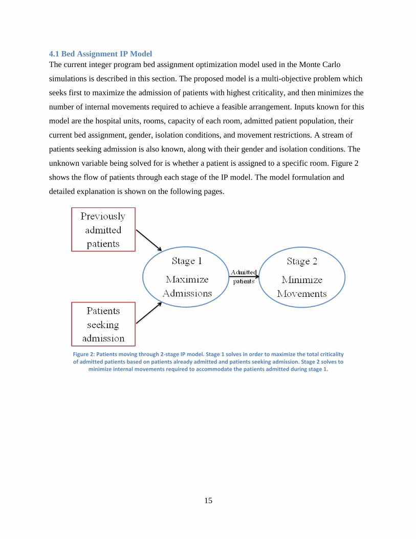
4.1 Bed Assignment IP Model
The current integer program bed assignment optimization model used in the Monte Carlo
simulations is described in this section. The proposed model is a multi-objective problem which
seeks first to maximize the admission of patients with highest criticality, and then minimizes the
number of internal movements required to achieve a feasible arrangement. Inputs known for this
model are the hospital units, rooms, capacity of each room, admitted patient population, their
current bed assignment, gender, isolation conditions, and movement restrictions. A stream of
patients seeking admission is also known, along with their gender and isolation conditions. The
unknown variable being solved for is whether a patient is assigned to a specific room. Figure 2
shows the flow of patients through each stage of the IP model. The model formulation and
detailed explanation is shown on the following pages.
Figure 2: Patients moving through 2-stage IP model. Stage 1 solves in order to maximize the total criticality of admitted patients based on patients already admitted and patients seeking admission. Stage 2 solves to
minimize internal movements required to accommodate the patients admitted during stage 1.

16
Sets
𝑈: 𝑢𝑛𝑖𝑡𝑠 𝑖𝑛 𝑡ℎ𝑒 ℎ𝑜𝑠𝑝𝑖𝑡𝑎𝑙
𝑃𝐴𝑢: 𝑝𝑎𝑡𝑖𝑒𝑛𝑡𝑠 𝑐𝑢𝑟𝑟𝑒𝑛𝑡𝑙𝑦 𝑎𝑑𝑚𝑖𝑡𝑡𝑒𝑑 𝑡𝑜 𝑢𝑛𝑖𝑡 𝑢 ∈ 𝑈
𝑃𝑁𝑢: 𝑝𝑎𝑡𝑖𝑒𝑛𝑡𝑠 𝑠𝑒𝑒𝑘𝑖𝑛𝑔 𝑎𝑑𝑚𝑖𝑠𝑠𝑖𝑜𝑛 𝑡𝑜 𝑢𝑛𝑖𝑡 𝑢 ∈ 𝑈
𝑃: 𝑠𝑒𝑡 𝑜𝑓 𝑎𝑙𝑙 𝑝𝑎𝑡𝑖𝑒𝑛𝑡𝑠, ∪𝑢 ∈ 𝑈 (𝑃𝑁𝑢 ∪ 𝑃𝐴𝑢)
𝐼: 𝑠𝑒𝑡 𝑜𝑓 𝑖𝑠𝑜𝑙𝑎𝑡𝑖𝑜𝑛 𝑐𝑜𝑛𝑑𝑖𝑡𝑖𝑜𝑛𝑠
𝐺: 𝑠𝑒𝑡 𝑜𝑓 𝑔𝑒𝑛𝑑𝑒𝑟𝑠
𝑇: 𝑠𝑒𝑡 𝑜𝑓 𝑡𝑟𝑖𝑎𝑔𝑒 𝑟𝑜𝑜𝑚𝑠
𝐷: 𝑠𝑒𝑡 𝑜𝑓 𝑑𝑖𝑠𝑐ℎ𝑎𝑟𝑔𝑒 𝑟𝑜𝑜𝑚𝑠
𝑅𝑠: 𝑠𝑒𝑡 𝑜𝑓 𝑠𝑝𝑒𝑐𝑖𝑎𝑙 𝑡𝑟𝑖𝑎𝑔𝑒/𝑑𝑖𝑠𝑐ℎ𝑎𝑟𝑔𝑒 𝑟𝑜𝑜𝑚𝑠, 𝑇 ∪ 𝐷
𝑅𝑈𝑢: 𝑠𝑒𝑡 𝑜𝑓 𝑟𝑜𝑜𝑚𝑠 𝑓𝑜𝑟 𝑎 𝑠𝑝𝑒𝑐𝑖𝑓𝑖𝑐 𝑢𝑛𝑖𝑡 𝑢 ∈ 𝑈
𝑅: 𝑠𝑒𝑡 𝑜𝑓 𝑎𝑙𝑙 𝑟𝑜𝑜𝑚𝑠 𝑖𝑛 ℎ𝑜𝑠𝑝𝑖𝑡𝑎𝑙, ∪𝑢 ∈ 𝑈 (𝑅𝑠 ∪ 𝑅𝑢)
Parameters
𝑏𝑗: 𝑛𝑢𝑚𝑏𝑒𝑟 𝑜𝑓 𝑏𝑒𝑑𝑠 𝑎𝑣𝑎𝑖𝑙𝑎𝑏𝑙𝑒 𝑖𝑛 𝑟𝑜𝑜𝑚 𝑗 ∈ 𝑅
𝑔𝑖: 𝑔𝑒𝑛𝑑𝑒𝑟 𝑜𝑓 𝑝𝑎𝑡𝑖𝑒𝑛𝑡 𝑖 ∈ 𝑃
𝑙𝑖: 𝑖𝑠𝑜𝑙𝑎𝑡𝑖𝑜𝑛 𝑐𝑜𝑛𝑑𝑖𝑡𝑖𝑜𝑛 𝑜𝑓 𝑝𝑎𝑡𝑖𝑒𝑛𝑡 𝑖 ∈ 𝑃
𝑐𝑖: 𝑐𝑟𝑖𝑡𝑖𝑐𝑎𝑙𝑖𝑡𝑦 𝑙𝑒𝑣𝑒𝑙 𝑜𝑓 𝑝𝑎𝑡𝑖𝑒𝑛𝑡 𝑖 ∈ 𝑃, 𝑑𝑒𝑓𝑎𝑢𝑙𝑡 0
Δ𝑖: 𝑚𝑜𝑣𝑒𝑚𝑒𝑛𝑡 𝑟𝑒𝑠𝑡𝑟𝑖𝑐𝑡𝑖𝑜𝑛 𝑓𝑙𝑎𝑔 {0; 𝑝𝑎𝑡𝑖𝑒𝑛𝑡 𝑖 ∈ 𝑃 𝑐𝑎𝑛 𝑏𝑒 𝑚𝑜𝑣𝑒𝑑
1; 𝑝𝑎𝑡𝑖𝑒𝑛𝑡 𝑖 ∈ 𝑃 𝑐𝑎𝑛𝑛𝑜𝑡 𝑏𝑒 𝑚𝑜𝑣𝑒𝑑
𝑦𝑖𝑗′ : 𝑝𝑟𝑒𝑣𝑖𝑜𝑢𝑠 𝑙𝑜𝑐𝑎𝑡𝑖𝑜𝑛 𝑓𝑙𝑎𝑔 {0; 𝑝𝑎𝑡𝑖𝑒𝑛𝑡 𝑖 ∈ 𝑃 𝑤𝑎𝑠 𝑛𝑜𝑡 𝑝𝑟𝑒𝑣𝑖𝑜𝑢𝑠𝑙𝑦 𝑎𝑠𝑠𝑖𝑔𝑛𝑒𝑑 𝑡𝑜 𝑟𝑜𝑜𝑚 𝑗′ ∈ 𝑅
1; 𝑝𝑎𝑡𝑖𝑒𝑛𝑡 𝑖 ∈ 𝑃 𝑤𝑎𝑠 𝑝𝑟𝑒𝑣𝑖𝑜𝑢𝑠𝑙𝑦 𝑎𝑠𝑠𝑖𝑔𝑛𝑒𝑑 𝑡𝑜 𝑟𝑜𝑜𝑚 𝑗′ ∈ 𝑅
𝛼𝑗′𝑗: 𝑡𝑟𝑎𝑛𝑠𝑓𝑒𝑟 𝑝𝑒𝑛𝑎𝑙𝑡𝑦 𝑓𝑜𝑟 𝑚𝑜𝑣𝑒𝑚𝑒𝑛𝑡 𝑓𝑟𝑜𝑚 𝑟𝑜𝑜𝑚 𝑗′ ∈ 𝑅 𝑡𝑜 𝑟𝑜𝑜𝑚 𝑗 ∈ 𝑅
𝑎𝑖: 𝑎𝑑𝑚𝑖𝑠𝑠𝑖𝑜𝑛 𝑓𝑙𝑎𝑔 {0; 𝑝𝑎𝑡𝑖𝑒𝑛𝑡 𝑖 ∈ 𝑃 𝑖𝑠 𝑛𝑜𝑡 𝑎𝑑𝑚𝑖𝑡𝑡𝑒𝑑
1; 𝑝𝑎𝑡𝑖𝑒𝑛𝑡 𝑖 ∈ 𝑃 𝑖𝑠 𝑎𝑑𝑚𝑖𝑡𝑡𝑒𝑑
𝑝𝑖𝑢: 𝑐𝑜𝑠𝑡 𝑓𝑜𝑟 𝑎𝑠𝑠𝑖𝑔𝑛𝑖𝑛𝑔 𝑝𝑎𝑡𝑖𝑒𝑛𝑡 𝑖 ∈ 𝑃 𝑡𝑜 𝑢𝑛𝑖𝑡 𝑢 ∈ 𝑈
𝑑𝑐: 𝑑𝑒𝑐𝑒𝑛𝑡𝑟𝑎𝑙𝑖𝑧𝑒𝑑 𝑓𝑙𝑎𝑔 {0; ℎ𝑜𝑠𝑝𝑖𝑡𝑎𝑙 𝑢𝑠𝑒𝑠 𝑐𝑒𝑛𝑡𝑟𝑎𝑙𝑖𝑧𝑒𝑑 𝑠𝑜𝑙𝑣𝑖𝑛𝑔
1; ℎ𝑜𝑠𝑝𝑖𝑡𝑎𝑙 𝑢𝑠𝑒𝑠 𝑑𝑒𝑐𝑒𝑛𝑡𝑟𝑎𝑙𝑖𝑧𝑒𝑑 𝑠𝑜𝑙𝑣𝑖𝑛𝑔
Variables
𝑥𝑖𝑗 : {0; 𝑝𝑎𝑡𝑖𝑒𝑛𝑡 𝑖 ∈ 𝑃 𝑖𝑠 𝑛𝑜𝑡 𝑎𝑠𝑠𝑖𝑔𝑛𝑒𝑑 𝑡𝑜 𝑟𝑜𝑜𝑚 𝑗 ∈ 𝑅
1; 𝑝𝑎𝑡𝑖𝑒𝑛𝑡 𝑖 ∈ 𝑃 𝑖𝑠 𝑎𝑠𝑠𝑖𝑔𝑛𝑒𝑑 𝑡𝑜 𝑟𝑜𝑜𝑚 𝑗 ∈ 𝑅
𝛿ℎ𝑗 : {0; 𝑔𝑒𝑛𝑑𝑒𝑟 ℎ ∈ 𝐺 𝑖𝑠 𝑛𝑜𝑡 𝑝𝑟𝑒𝑠𝑒𝑛𝑡 𝑖𝑛 𝑟𝑜𝑜𝑚 𝑗 ∈ 𝑅 | 𝑏𝑗 > 1
1; 𝑔𝑒𝑛𝑑𝑒𝑟 ℎ ∈ 𝐺 𝑖𝑠 𝑝𝑟𝑒𝑠𝑒𝑛𝑡 𝑖𝑛 𝑟𝑜𝑜𝑚 𝑗 ∈ 𝑅 | 𝑏𝑗 > 1

17
𝛾𝑖𝑗 : {0; 𝑖𝑠𝑜𝑙𝑎𝑡𝑖𝑜𝑛 𝑐𝑜𝑛𝑑𝑖𝑡𝑖𝑜𝑛 𝑖 ∈ 𝐼 𝑖𝑠 𝑛𝑜𝑡 𝑝𝑟𝑒𝑠𝑒𝑛𝑡 𝑖𝑛 𝑟𝑜𝑜𝑚 𝑗 ∈ 𝑅 | 𝑏𝑗 > 1
1; 𝑖𝑠𝑜𝑙𝑎𝑡𝑖𝑜𝑛 𝑐𝑜𝑛𝑑𝑖𝑡𝑖𝑜𝑛 𝑖 ∈ 𝐼 𝑖𝑠 𝑝𝑟𝑒𝑠𝑒𝑛𝑡 𝑖𝑛 𝑟𝑜𝑜𝑚 𝑗 ∈ 𝑅 | 𝑏𝑗 > 1
𝛽𝑖𝑗′𝑗: 𝑚𝑜𝑣𝑒𝑚𝑒𝑛𝑡 𝑝𝑒𝑛𝑎𝑙𝑡𝑦 𝑓𝑜𝑟 𝑝𝑎𝑡𝑖𝑒𝑛𝑡 𝑖 ∈ 𝑃 𝑓𝑟𝑜𝑚 𝑟𝑜𝑜𝑚 𝑗′ ∈ 𝑅 𝑡𝑜 𝑗 ∈ 𝑅

18
Stage 1
Objective
Maximize: ∑ ∑ 𝑐𝑖𝑥𝑖𝑗𝑗∈𝑅\𝑅𝑠𝑖∈𝑃
Constraints:
(1) ∑ 𝑥𝑖𝑗 = 1𝑗∈𝑅\𝑅𝑠 ∀ 𝑢 ∈ 𝑈, 𝑖 ∈ 𝑃𝐴𝑢
(2) ∑ 𝑥𝑖𝑗 = 1𝑗∈𝑅\𝐷 ∀ 𝑢 ∈ 𝑈, 𝑖 ∈ 𝑃𝑁𝑢
(3) 𝑥𝑖𝑗 ≤ 𝛿𝑔𝑖𝑗 ∀ 𝑖 ∈ 𝑃, ∀ 𝑗 ∈ 𝑅 | 𝑏𝑗 > 1
(4) 𝑥𝑖𝑗 ≤ 𝛾𝑙𝑖𝑗 ∀ 𝑖 ∈ 𝑃, ∀ 𝑗 ∈ 𝑅 | 𝑏𝑗 > 1
(5) ∑ 𝛿ℎ𝑗 = 1ℎ∈𝐺 ∀ 𝑗 ∈ 𝑅\𝑅𝑠 | 𝑏𝑗 > 1
(6) ∑ 𝛾𝑖𝑗 = 1𝑖∈𝐼 ∀ 𝑗 ∈ 𝑅\𝑅𝑠 | 𝑏𝑗 > 1
(7) ∑ 𝑥𝑖𝑗 ≤ 𝑏𝑗𝑖∈𝑃 ∀ 𝑗 ∈ 𝑅
(8) 𝑥𝑖𝑗 = 0 ∀ 𝑢 ∈ 𝑈, 𝑖 ∈ 𝑃𝐴𝑢 | 𝑗 ∈ 𝑇
(9) ∑ 𝑥𝑖𝑗 = 0𝑗∈𝑅|(𝑏𝑗=1,𝑗≠𝑗′) ∀ 𝑖 ∈ 𝑃, ∀ 𝑗′ ∈ 𝑅 | (𝑏𝑗′ = 1, 𝑦𝑖𝑗′ = 1)
(10) 𝑥𝑖𝑗 ≥ Δ𝑖𝑦𝑖𝑗 ∀ 𝑖 ∈ 𝑃, ∀ 𝑗 ∈ 𝑅
(11) ∑ 𝑥𝑖𝑗 = 1𝑗∈𝑅𝑈𝑢∪ 𝑇 ∀ 𝑢 ∈ 𝑈, 𝑖 ∈ (𝑃𝐴𝑢 ∪ 𝑃𝑁𝑢) | 𝑑𝑐 = 1

19
Stage 2
Objective
Minimize: ∑ ∑ ∑ 𝛽𝑖𝑗′𝑗𝑗∈𝑅𝑗′∈𝑅𝑖∈𝑃|𝑎𝑖=1
Constraints:
(5) - (7), (10) from previous stage
(12) ∑ 𝑥𝑖𝑗 = 1𝑗∈𝑅\𝑅𝑠 ∀ 𝑢 ∈ 𝑈, 𝑖 ∈ 𝑃𝐴𝑢 | 𝑎𝑖 = 1
(13) ∑ 𝑥𝑖𝑗 = 1𝑗∈𝑅\𝐷 ∀ 𝑢 ∈ 𝑈, 𝑖 ∈ 𝑃𝑁𝑢 | 𝑎𝑖 = 1
(14) 𝑥𝑖𝑗 ≤ 𝛿𝑔𝑖𝑗 ∀ 𝑖 ∈ 𝑃, ∀ 𝑗 ∈ 𝑅 | 𝑏𝑗 > 1 | 𝑎𝑖 = 1
(15) 𝑥𝑖𝑗 ≤ 𝛾𝑙𝑖𝑗 ∀ 𝑖 ∈ 𝑃, ∀ 𝑗 ∈ 𝑅 | 𝑏𝑗 > 1 | 𝑎𝑖 = 1
(16) 𝑥𝑖𝑗 = 0 ∀ 𝑢 ∈ 𝑈 , 𝑖 ∈ 𝑃𝐴𝑢 | (𝑎𝑖 = 1, 𝑗 ∈ 𝑇)
(17) ∑ 𝑥𝑖𝑗 = 0𝑗∈𝑅|(𝑏𝑗=1,𝑗≠𝑗′) ∀ 𝑖 ∈ 𝑃, ∀ 𝑗′ ∈ 𝑅 | (𝑎𝑖 = 1, 𝑏𝑗′ = 1, 𝑦𝑖𝑗′ = 1)
(18) ∑ 𝑥𝑖𝑗 = 1𝑗∈𝑅𝑈𝑢∪ 𝑇 ∀ 𝑢 ∈ 𝑈, ∀ 𝑖 ∈ (𝑃𝐴𝑢 ∪ 𝑃𝑁𝑢) | (𝑎𝑖 = 1, 𝑑𝑐 = 1)
(19) 𝛽𝑖𝑗′𝑗 = 𝛼𝑗′𝑗𝑥𝑖𝑗 ∀ 𝑖 ∈ 𝑃, ∀ 𝑗, 𝑗′ ∈ 𝑅\𝑅𝑠 | 𝑦𝑖𝑗′ = 1
(20) 𝛽𝑖𝑗′𝑗 = 𝑝𝑖𝑢𝑥𝑖𝑗 ∀ 𝑢 ∈ 𝑈, ∀ 𝑖 ∈ 𝑃, ∀ 𝑗′ ∈ 𝑇, ∀ 𝑗 ∈ 𝑅𝑈𝑢 |(𝑎𝑖 = 1, 𝑦𝑖𝑗′ = 1)
(21) ∑ 𝑥𝑖𝑗𝑗∈𝑅\𝑅𝑠 = 𝑎𝑖 ∀ 𝑖 ∈ 𝑃
(22) 𝛽𝑖𝑗′𝑗 ≥ 0
20
4.2 Model Explanation
This model solves in two stages. First, it decides whom to admit in order to maximize the
criticality of patients in the system, ensuring the most ill receive treatment first. After choosing
which patients to admit, a second stage makes bed assignments in order to minimize patient
movements. A single patient movement from one room to another in the same unit is considered
one movement.
It is not always possible to accommodate patients in their preferred unit due to space restrictions.
When patients are placed in a non-preferred unit, it incurs a penalty, increasing the cost of that
movement. This allows the system to move patients to non-optimal units, but incentivizes
making internal movements in the same unit.
Constraints (1) and (12) ensure that any patient previously admitted occupies a bed in the
hospital, and is not assigned back to triage or discharged prematurely. Constraints (2) and (13)
ensure that patients seeking admission are either given a bed assignment, or remain in triage
awaiting bed assignment. Constraints (3) and (14) ensure that a patient is only assigned to a room
if it is empty or a matching gender is present in the room. Similarly, constraints (4) and (15)
ensure that a patient is only assigned to a room if it is empty or a matching isolation requirement
is present in the room. Constraint (5) ensures that only one gender is present in a room.
Constraint (6) ensures that only one isolation condition is present in a room. Constraint (7)
ensures that the total number of patients assigned to a room does not exceed the bed capacity of
the room. Constraints (8) and (16) make sure that all patients previously admitted are not
assigned back to the triage room. Constraints (9) and (17) ensure that a patient occupying a
single room is not reassigned to a different single room. Constraint (10) prevents patients being
moved who have been flagged ineligible for movement (e.g. when restricting patient movements
to once per day). Constraints (11) and (18) are used in decentralized admission policy, allowing
patients only to be assigned to rooms within their current unit. Constraint (19) defines the penalty
movement for moving previously admitted patient to a new room. Similarly, constraint (20)
defines the penalty for admitting a patient to a non-preferred unit. Constraint (21) ensures that
any patient selected for admission in the first problem is assigned a room. Finally constraint (22)
ensures non-negativity on the movement variables, which allows their sum to be minimized.

21
4.3 Experiments Overview
This study relies on a Monte Carlo simulation that solves the integer program bed assignment
model for different problem instances of a set of experimental scenarios. The model tests
different bed assignment policies in order to answer the questions set out in the problem
statement. For each experimental scenario in the following sections, there are 50 replications of
365 days, with a 100 day warm up period prior to data collection in each replication. This results
in 50 years of data for each arrangement. During each scenario patient demand is sampled from
arrival rate and length-of-stay distributions. Using these distributions, we apply Little’s law to
predict the long-term number of patients in the multi-occupancy unit. Arrival and length-of-stay
distributions are chosen to mimic situations where the expected patients in the system are 18, 24,
28, 31, and 38 patients. Table 1 shows the distribution names and the corresponding expected
number of patients for that distribution. The original distribution (PCU38A) was estimated using
the distributions from Cignarale et al. [42], which was empirically acquired from an actual
hospital unit. The remaining distributions were created by modifying the arrival rate distribution
to reach a certain expected number of patients, while maintaining the same variance as the
original distribution.
The following data are collected at each time interval: number of internal movements, total
number of patients admitted to each unit, unit utilization rate, criticality level for each unit and
the entire hospital, number of discharged patients, number of patients leaving without being seen
(their discharge date having come before a room became available for them), and the penalty
value, which only applies to centralized admissions as a measure of placing patients in a non-
preferred unit. Figure 3 illustrates an overview of the simulation for each experimental scenario
Distribution Name Expected Number of Patients
PCU18A 18.14
PCU24A 23.99
PCU28A 28.13
PCU31A 31.09
PCU38A 38.75
Patient Demand Distributions
Table 1: Expected number of patients for each unit demand distribution

22
At the beginning of each replication patient demand is randomly generated for the entire length
of the replication. Each time interval begins by discharging any patient whose discharge time has
arrived. Following this the remaining admitted patients and patients seeking admission at the
current time are fed into stage one of the bed assignment IP model. Then the admitted patients
are sent to the second stage of the IP model for bed assignment and the necessary assignments
are made. If the warm-up period has been completed then results are collected prior to advancing
to the next time interval. The process repeats for the next time interval, starting with discharging
patients. After all the time intervals have been completed the replication advances causing a new
stream of random patient demand to be generated. This process repeats itself until all replications
are complete at which point the simulation ends for the current experimental scenario.
To understand how different admissions policies affect a unit, it is necessary first to analyze units
individually, evaluating how they function independent of the whole. It then becomes possible to
explore how multiple units within the entire hospital function, and to determine whether they run
more efficiently under a decentralized (each unit making their own decisions) or centralized
(data from every unit considered in the decision making process) admission procedure. Figure 4
shows the three overarching themes of our experiments and how the results of earlier
experiments are utilized in the later experiments.
Figure 3: Simulation overview for each scenario

23
Figure 4: Overview of experiments
Experiment A focuses on varying patient demand for the unit and modifying the number of beds
contained in each room. This determines an optimal room configuration for each unit, which is
then used to create scenarios for later experiments. Experiment B determines if there is an
optimal time interval that should pass before making admission decisions. Both experiments A
and B utilize a single unit. Experiment C incorporates the previous results as it looks at a multi-
unit hospital using both decentralized and centralized admitting policies. This experiment
determines if there is an advantage when units pool bed capacities, allowing patients to be
admitted to any unit instead of only their preferred unit.
4.4 Assumptions
A number of assumptions are adopted in this study. The arrival rate and length-of-stay
distributions are known and invariable for each scenario. Each unit is allocated a number of
rooms that can either be configured as a single or double room. However, the room type does not
change from single to double or vice-versa during the simulation. No patient admission requests
are known prior to their arrival in the system. The patient’s length of stay, criticality, and
isolation conditions are fixed and do not change during a simulation run, even if a patient
admission is delayed. There are 8 isolation conditions and each have an equal likelihood of
occurring. Experiments A and B are run as a single unit simulation. During experiment A the
model is used to generate bed assignments only once per day. Additionally, this study does not
consider factors such as disease spread within the hospital, patients who have multiple isolation
conditions, or staffing models.

24
5. Experiments and Results
The following section looks at the setup and results for each of the previously described three
experiments.
5.1 Experiment A: Unit Demand
Setup
In order to answer questions about the effect of unit demand patterns, the arrival rate, length-of-
stay distributions, and bed configurations are varied. A single unit with 18 rooms is used and the
bed configuration changed to consider all possible room configurations, from 18 single rooms to
18 double rooms. This gives a minimum unit capacity of 18 patients (18 single rooms) and a
maximum unit capacity of 36 patients (18 double rooms). These capacities along with the
expected number of patient options lead to patient demand varying between 50% and 200% of
unit capacity, depending on bed configuration. These values also create expected unit utilization
rates that have been shown in the literature to affect HAIs and which match actual hospital
utilization averages [52-54]. Figure 5 shows the available options for each experimental scenario,
choosing one unit demand and one room arrangement for each scenario.
This experimental setup results in 95 unique scenarios combining the different demand and room
arrangements. Each scenario is simulated for 50 replications with a 100 day warm up period and
365 days of data collection resulting in 23,250 days simulated. Counting all 95 scenarios, this
results in a total of 2,208,750 days simulated.
Single Rooms 0 1 2 3 4 5 6 7 8 9 10 11 12 13 14 15 16 17 18
Double Rooms 18 17 16 15 14 13 12 11 10 9 8 7 6 5 4 3 2 1 0
Unit DemandChoose one demand
pattern
Choose single/double
room pair
Experiment A Experimental Scenarios
PCU24A PCU28A PCU31A PCU38APCU18A
Figure 5: Options for experiment A scenarios. There are 2 factors, with 5 levels for unit demand and 19 levels for room configuration of the unit, giving 95 total experimental scenarios.

25
Results for Experiment A: Unit Demand
The results for varying unit demand and the number of beds per room are shown in the following
section. Figure 6 shows the average number of internal movements per day as a function of the
number of single rooms, organized by each unit demand distribution. A 95% confidence interval
is drawn around each datum point.
As can be seen in the graph, when there is a mix of single and double rooms we see a higher
number of internal movements. In a unit with 18 single rooms there are 0 internal movements,
since in such a unit there is no need for rearrangement. The drawback however is that such a
unit’s capacity is severely limited. In units with only double rooms we also find a local minimum
for the number of internal movements per day, since in such units there is a higher chance for a
patient to match with a room before do any rearrangements. This suggests that maximizing the
number of double rooms allows a unit to treat more patients while also reducing the number of
internal movements.
Figure 6: Average number internal movements per day vs. room configuration; by unit demand. 95% confidence intervals also shown.

26
Figure 7 shows the average number of movements per day as a function of the utilization
percentage (percent of available beds currently occupied). This figure shows results for differing
unit demand distributions.
As can be seen in this graph, once the utilization rate begins to surpass 80%, the number of
internal movements and the variability in the number of movements begins to increase
significantly. This suggests that in order to reduce the number of internal movements it is
advantageous to keep average unit utilization under 80%.
Figure 7: Average number of internal movements per day vs. utilization percentage; by unit demand

27
Figure 8 shows the number of patients who leave-without-being-seen (LWBS) per day as a
function of the utilization rate, again displayed by unit demand distribution. LWBS is a measure
of the unit’s failure to accommodate patients due to insufficient capacity. In our model, a patient
whose discharge time comes prior to their being selected for admission causes them to leave-
without-being-seen.
This graph shows a moderate increase in the LWBS rate once utilization passes 80%, however
there is a significant increase the rate of patients leaving after unit utilization passes 90%.
Therefore, the ability of the unit to accommodate patients suffers as utilization increases,
meaning that it is preferable to keep utilization less than 90%.
Figure 8: LWBS per day vs. utilization percentage; by unit demand

28
Figure 9 plots the utilization percentage as a function of the number of single rooms, organized
by unit demand distribution.
80% and 90% utilization cutoff lines are shown on this graph based on data from Figures 7 and 8
which suggested that at these utilization levels unit operations begin to be significantly impacted.
Using these cutoff lines we are able to find where a specific unit demand pattern reaches an
average utilization percentage and then determine the ideal room arrangement. This is shown in
Figure 10.
Figure 9: Utilization percentage vs. room configuration; by unit demand

29
Figure 10: Determining ideal room capacity for a specified utilization percentage
This graph shows the intersection of the PCU38A demand distribution and 90% average
utilization. From this point, drawing a line down to the x-axis indicates that arranging the unit
with 3 single rooms and 15 double rooms should result in no more than 90% average utilization.
Increasing the number of double rooms leads to lower average utilization. This graph can be used
for any desired utilization percentage by simply plotting a horizontal line at the desired
utilization percentage and then finding where it intersects the distribution being assumed.
Additionally, using the bed assignment IP model, this graph could be generated for any number
of total rooms and unit demand distributions. Ultimately, this graph is a powerful tool as it gives
unit managers a way to balance the tradeoffs between room configurations, unit capacity,
internal movements, and any other metric which is dependent on utilization percentage of the
unit.

30
Unit Demand Utilization Rate Single Rooms Double Rooms
80% 7 11
90% 13 5
80% 3 15
90% 9 9
80% 1 17
90% 7 11
PCU24A
PCU28A
PCU31A
Unit Arrangements
Figure 11: Room arrangements for unit and utilization pairs. Room arrangement determined using method explained during experiment A, figure 10.
5.2 Experiment B: Batching
Setup
In experiment A, admissions took place once a day. The frequency of admissions can be
increased by reducing the time interval between batch admissions. In order to explore the effect
of the time interval between batch admissions, we change the number of times the problem is
solved during each day. The arrival and length-of-stay distribution choices are reduced to mimic
situations where the expected patients in the system are 24, 28, and 31 patients. For each of these
distribution we choose the room configuration corresponding to 80% and 90% utilization, as
found during experiment A. Figure 11 shows the arrangement of rooms within the unit for each
demand and utilization pair. These choices were made based on the data in Figure 10.
The different time intervals between batch admissions considered in experiment B are: every
time a patient arrives, every time a patient arrives or is discharged, every hour, every 4 hours,
every 8 hours, and every 24 hours. Since it is inconvenient and impractical to repeatedly move
the same patient around, even if doing so yields the optimal solution, we allow two different
patient movement conditions: one allowing an individual patient to be assigned to a new spot an
unlimited number of times per day, and the other restricting individual patients to a new bed
assignment once per day. Figure 12 shows the available conditions for each scenario.

31
This experimental setup results in 72 unique scenarios combining the different levels of each
factor. Each scenario is simulated for 50 replications with a 100 day warm up period and 365
days of data collection resulting in 23,250 days simulated. Counting all 72 scenarios this results
in a total of 1,674,000 days simulated.
Results for Experiment B: Batching
The results for varying time intervals to batch admissions are shown in the following section.
The time intervals we chose to experiment with consist of both static and variable periods of
time. Under the static time intervals, it is known exactly how many times the model will be
solved each day, since the same amount of time passes between each solution. This does not hold
true for the variable time intervals, which are dependent on patient arrivals and discharges. Table
2 shows the average number of times the model is solved under each distribution, time interval,
and movement restriction scenario.
For all the static conditions, the number of times the model is solved each day stays the same
regardless of which distribution is used. For the variable time intervals, the number of times the
model is solved per day varies based on both the distribution and time interval selected. For the
variable time intervals, the model is solved more times per day when using both the arrival and
Interval Type Static Static Static Static Variable Variable Variable Variable
Time Interval Hourly 4 hours 8 hours Daily On Arrival On Arrival On On Arrival On Arrival On
Movement Restriction Both Both Both Both No Restriction No Restriction Restricted Restricted
PCU24A 80% Utilization 24 6 3 1 3.1 4.7 3.1 4.6
PCU24A 90% Utilization 24 6 3 1 3.2 4.7 3.1 4.7
PCU28A 80% Utilization 24 6 3 1 2.9 5.3 2.9 5.3
PCU28A 90% Utilization 24 6 3 1 2.9 5.3 2.9 5.3
PCU31A 80% Utilization 24 6 3 1 2.9 5.9 2.9 5.9
PCU31A 90% Utilization 24 6 3 1 2.9 5.9 2.9 5.8
Average Number of Model Solves/Day
Average Number of Times/Day Batch Admissions are Solved for Each Scenario
Dis
trib
uti
on
Table 2: Average number of times the model is solved per day
4 hours 8 hours Daily
Choose oneMovement
RestrictionMovement restricted No movement restriction
Experiment B Experimental Scenarios
Choose one Unit Demand PCU24A PCU28A PCU31A
Choose one Utilization % 80% 90%
Choose one Time Interval On ArrivalOn Arrival
On DischargeHourly
Figure 12: Options for experiment B scenarios. There are 4 factors, with 3 levels for unit demand, 2 levels for utilization percentage, 6 levels for time interval, and 2 levels for movement restriction, giving 72 unique experimental scenarios.

32
discharge of patients as triggers for the solving the model. The values in this table are important
going forward, as a number of the graphs will use the average number of model solves per day as
the independent variable, which allows for easier identification of trends in the data.
Additionally, since the mechanism which triggers a model solve in the variable time intervals is
different from that in the static time intervals, the data points for variable time intervals will be
plotted, but excluded from any trend lines drawn for the static intervals.
The number of internal movements as a function of the average number of model solutions per
day is plotted in Figure 13. The graph is sorted by distribution. The no movement restriction
policy is on the left, and the movement restriction policy on the right.
The trend seen here is that as the model is solved with increasing frequency there are more
internal movements. This is to be expected as additional model solves per day result in more
opportunities to rearrange patients. Restrictions on patient movement result in the same trend in
both cases, but there is a very slight decrease, approximately 0.2 movements per day, when
patients are restricted to being moved only once per day. Across the board, solving hourly results
in an average of 1.2 more internal movement movements per day than solving daily. When using
a varying time interval, the number of internal movements is more than a static time interval with
the same number of solutions per day. This is likely due to an additional level of randomness in
varying time intervals, in which the number of model solutions varies from day to day.
Figure 13: Average number of internal movements vs. average model solutions per day

33
Figure 14 shows the average unit criticality as a function of the average number of model solves
per day. Unit criticality is the aggregated criticality level for all patients admitted to the unit. A
higher criticality level indicates that more severely ill patients are being treated. Once again the
graphs are plotted by distribution, and the movement restriction graph is on the right.
These graphs show that average criticality of patients in a unit differs very little on the basis of
frequency of solution. For lower volume units the trend tends to be a small boost in unit
criticality when implementing an additional time interval which then drops off with more
frequent solutions. In a higher volume unit the trend tends to increase slightly, with criticality
generally remaining the same. It is to be expected that high demand, high utilization units trend
upwards, as more frequent solutions allow more opportunities to evaluate patients and get the
most critical admitted. However, when the unit has lower utilization, the trend may go
downwards. Looking at PCU31A 80% utilization as an example, the increased solution intervals
lead to patients being discharged earlier, but less utilization could result in an empty bed which
then reduces unit criticality. Comparing movement restriction policies, there are no significant
differences between the two in average unit criticality. Across all distributions, the variable time
intervals outperform the static time intervals at the same number of solutions per day. Logically
this should be expected, since the variable time intervals are driven by patient demand patterns.
Solving when a patient arrives means that the patient will be admitted immediately if there is a
bed available. Solving when a patient is discharged means that if there are patients waiting, one
of them will get the open bed immediately. This results in more beds being filled faster, thus
Figure 14: Average unit criticality vs. average model solutions per day

34
driving up the occupancy of the units, and in turn the unit’s criticality level. However, there does
not tend to be a significant change in the unit’s criticality level as a result from admitting more or
less frequently. As long as the unit is able to adequately meet its patient demand, the unit
manager can decide what time interval to use in making bed assignments, balancing the tradeoff
between that time interval and the changing number of internal movements.
The LWBS rate vs. average number of model solves per day is shown in Figure 15. This graph is
sorted by distribution and the restricted movements graph is once again on the right.
Increased solution frequency results in fewer patients leaving without being seen. This is what
should be expected to happen, since evaluating the patient queue more frequently means patients
are being discharged sooner, freeing up beds. Patients are also being admitted earlier when beds
are open. When solving once per day, there could be close to 24 hours between the time a bed
opens up and when a patient is finally admitted to it. That is 23 more hours that the patient has to
choose to LWBS compared to the hourly solution interval. If a bed opens up for a patient, there
is at maximum one hour between that bed becoming available and the patient getting it. Having a
restriction on movements per day does have a slight negative impact on the LWBS rate, leading
it to increase. This happens because a movement restriction policy limits some of the potential
rearrangements, making it harder for a patient to get into the unit. Any policy that makes it
harder to rearrange patients and admit new patients has a negative impact on the unit’s ability to
Figure 15: Average LWBS/day vs. average model solutions per day

35
meet patient demand. The variable time interval data shows mixed results compared to static
time intervals. When solving solely on patient arrival, the LWBS rate tends to be higher than the
static time interval equivalent. When solving on patient arrival or discharge, the LWBS rate is
sometimes higher than the static time interval equivalent, but in other cases lower. This
inconsistency is likely due the variability in the time intervals. Some days there may be a large
number of patients arriving and leaving, but other days a very small number. This may result in
large periods of time in which no one gets admitted, thus driving up the failure rate of the unit.
The clear trend from these graphs is that more frequent solutions with no restriction on patient
movement results in the unit better meeting patient demand.
Another consideration is the difficulty of implementing the different time interval policies. In
order to evaluate this we look at Figure 16, showing the variability in patient movements per day
on the basis of the average number of times batch admissions occur. A policy with high levels of
variability would be difficult to implement because it is hard to plan how many movements to
expect on a day-to-day basis. These graphs are sorted by distribution and the restricted
movement graph is on the right.
Note that movement variance increases with frequency of solution and is higher when a
restricted movement policy is in place. This is to be expected, as more frequent solutions yield
more opportunities to rearrange patients and a restriction on individual patient movements that
changes throughout the day makes it harder to know in advance how many movements will be
required for a particular rearrangement. At one time interval only one patient might be blocked,
Figure 16: Movement variance vs. average number of model solutions per day

36
at another five patients might be, which impacts the number of movements needed for the next
rearrangement. The “unknown” factor of how many patients are blocked from moving introduces
more randomness to the problem, thus increasing variability. The more important thing in this
graph however is the scale of the variability. Overall, variability in all scenarios is small, less
than 0.15. Even though there is a difference between the policies, the variability is so small as
not to have a significant impact, and so each policy would be practical to implement.
Once again the decision as to which policy is best comes down to tradeoffs between internal
movements and the ability of the unit to accommodate its patients. A policy that solves bed
assignments more frequently better meets the needs of patients at the cost of a very small
increase to the number of internal movements per day. Choosing to implement a policy to restrict
movement of individual patients to once per day does have a slight negative impact to unit
operations, however since the impact appears negligible and the benefit of increased patient
comfort from being moved around less easily outweighs the negative operational impact, it
seems a worthwhile constraint. Based on the data, our recommendation is to discharge patients
and make admission decisions using the IP model every hour.

37
5.3 Experiment C: Centralized Admission
Setup
In order to investigate the effect of centralized vs. decentralized admission policies; a
hypothetical 5 unit hospital is studied. Each hospital unit has one of the previous arrival and
length-of-stay distributions and its bed configuration is selected to ensure operation at 95%
utilization. The hospital setup is shown in Table 3.
Having all the units near maximum capacity allows us to isolate the difference between
centralized and decentralized admission policies. For a decentralized solution, when the unit is
full, all remaining patients need to be turned away until a spot opens up. In the centralized
solution, when the unit is full, patients may be admitted to a different unit in the hospital that is
not at capacity. By arranging the units with patient demand patterns and room configurations
which are known to cause high utilization, we create a “worst case” scenario in which individual
units are full the majority of the time. If the centralized policy works best in this extreme
scenario, it should work better in more relaxed scenarios with some units not at capacity.
These experiments are run under three different admission time interval policies from the
previous set of experiments. The time interval is either: hourly, on arrival, or on arrival and
discharge. Each experiment is solved using either a centralized approach or a decentralized
approach. In the case of the centralized approach, the penalty for admitting a patient outside their
preferred unit or moving a patient to a new unit will be set at 2. This means that the hospital
considers it double the amount of work to put a patient in a non-preferred unit over a preferred
unit. Figure 17 displays the possible experiment options.
Unit Name Distribution # Single Rooms # Double Rooms Total Beds
PCU0 PCU24A 16 2 20
PCU1 PCU24A 16 2 20
PCU2 PCU28A 12 6 24
PCU3 PCU28A 12 6 24
PCU4 PCU31A 10 8 26
Hospital Setup
Table 3: Units within hospital for centralized admission experiments

38
This experimental setup will result in 6 unique scenarios when combining the different demand
and room arrangements. Each scenario is simulated for 50 replications with a 100 day warm up
period and 365 days of data collection resulting in 23,250 days simulated. Considering all
possible scenarios results in a total of 139,500 days simulated.
Results for Experiment C: Centralized Admission
The results for using centralized admissions policies are shown in the following section. Figure
18 below, shows the average number of internal movements per day across the hospital with
respect to the different time intervals. The results are plotted by admitting policy with 95%
confidence intervals drawn around each value. Using a centralized admitting policy the average
Figure 18: Average internal movements per day for different centralized admitting policies, 95% confidence intervals also shown.
Experiment C Experimental Scenarios
Choose one Time Interval On ArrivalOn Arrival
On DischargeHourly
Choose one Policy Centralized Decentralized
Figure 17: Options for experiment C scenarios. There are 2 factors, with 3 levels for time interval and 2 levels for centralized admissions policy, giving 6 total experimental scenarios.

39
Figure 19: Average daily hospital utilization for different centralized admission policies, 95% confidence intervals also shown.
number of internal movements per day across the hospital is less than using a decentralized
policy. On average two less internal movements occur per day under the centralized admissions
policy. The 95% confidence intervals also show that this difference is statistically significant
since the intervals do not even come close to overlapping. Clearly a centralized admission policy
is superior for reduction of internal movements.
Figure 19 shows hospital bed utilization as a function of the time interval selected. The data are
plotted by centralized admitting policy and has 95% confidence intervals drawn around each
value.
Utilization of beds across the hospital is higher when using a centralized admitting policy. Under
the high patient demand patterns used for these experiments, utilization runs 4% higher when
using a centralized admission policy. This is once again a statistically significant difference and
means that the beds across the hospital are staying filled, but there can be beds going empty
under a decentralized policy even though there is demand for the empty beds.

40
Figure 20 shows the average LWBS rate with respect to different solution frequencies. The data
are again plotted by centralized admitting policy with 95% confidence intervals.
The LWBS rate is lower under a centralized admitting policy. More patients are admitted due to
more beds being available when pooling resources across all units. More patients admitted means
less are leaving without being seen. A centralized admitting policy results in a statistically
significant reduction in the LWBS rate. This means the hospital can better meet its patient
demand when it uses a centralized admitting policy.
Figure 20: LWBS rate for different centralized admitting policies, 95% confidence intervals also shown.

41
Last we want to ensure that these policies are not too difficult to implement. Figure 21 shows the
variability in the movements/day with respect to the different time intervals.
The centralized admitting policy results in less day-to-day variance for internal movements. This
is likely due to beds being available on a more consistent basis when they are pooled. Low
variance means that the number of internal movements per day are going to be relatively
consistent and there is not going to be days with significantly more internal movements required.
It is worth noting that the variance under both cases is still extremely low, so both policies are
reasonable to utilize without much difficulty.
A centralized admitting policy is more convenient than a decentralized approach. All of the
results support this, with the centralized policy leading to less internal movements, a lower
failure rate, and higher utilization when every unit is at capacity. It is also easier to implement
due to less variance in the number of internal movements. This matches what we expected would
happen since a centralized policy gives more options and flexibility to where a patient can be
placed to receive treatment.
Figure 21: Movements per day variance for different centralized admitting policies

42
6. Discussion
6.1 Unit Demand
There are a number of tradeoffs between internal movements, utilization, and patients
accommodated as the unit demand and room configuration are changed. If the goal is to
minimize the internal movement of admitted patients, which we expect would reduce infectious
disease acquisition rates, then it is optimal only to use single rooms. However, as shown in the
results, this may not be practical due to low capacity, high utilization concerns. For units that are
unable to utilize solely single rooms, the next best option to minimize internal movements is to
configure all rooms as double rooms. By minimizing internal movements, we expect that patients
will have less HAIs due to the role the patient movement can play in exposure to and contraction
of an infection. We do not prove that using this model causes less HAIs, however we propose a
tool which allows a unit to reduce their internal movements, which we expect would reduce
HAIs.
Using single rooms leads to high utilization of a unit. High utilization has been correlated with
increased hospital-acquired infection rates and medical errors [52, 53]. Minimizing internal
movements by increasing single rooms to reduce infection rates while in turn raising the
utilization rate of the unit may actually be counterproductive. Paradoxically, this could result in a
rise of infection rates due to the correlation between high unit utilization and HAIs, however it
should be noted the cause for the increase in HAIs under high utilization is not yet known.
Using double rooms allows for greater capacity and lower utilization while still providing the
flexibility to use a room as a single if needed. It also enables the unit to accommodate
unexpected surges in patient demand. Understandably, a unit could still wish to use some single
rooms. There have been studies suggesting the decreased costs from less nosocomial infections
cover the additional cost of operating a single room, as well as there being a net social benefit to
single room use [20, 21]. Additionally, hospitals can charge a cost differential for patients
requesting a single room if there is no medical necessity for their use of such a room [55].
Another option would be to use all double rooms, but implement a “blocking” policy on the
second bed in some of the rooms, allowing it to only be used if utilization reaches a certain
threshold. Ultimately, if the choice is made to use some single rooms, then it should be done

43
such that the expected bed utilization rate remains under 80%. Once a unit crosses the 80%
utilization threshold there is a significant increase in the rate of failure to accommodate patients.
It should be noted that this analysis was done for a generic isolated unit scenario. In these
simulations there was an equal chance of a patient having any one of eight different isolation
conditions, and the probability of a patient being a specific gender was set exactly at 50%. This
interpretation also did not consider factors like unit staffing, infectious disease spread among
patients, patients with multiple isolating conditions, and the role of the unit in a multi-unit
hospital where patients can be moved between units. The patient dynamics of a real-life unit
would vary considerably from the parameters used here.
Our goal was to determine an optimal bed configuration to reduce internal movements and thus
HAIs for the unit demand patterns. We found that the optimal bed configuration for a unit is
highly dependent on the how the unit prefers to manage the tradeoffs between internal
movements, patients accommodated, and utilization rates. Although we were unable to provide a
specific optimal bed configuration, we demonstrate that this model could be an effective tool for
a unit looking to analyze different bed arrangements, should they load in parameters specific to
their unit and ultimately determine the best bed configuration for their unit.
6.2 Batching
Changing the time interval over which to batch admission decisions also comes with tradeoffs.
The most prominent is between the number of internal movements and the unit LWBS (failure)
rate. More frequent solutions result in a decreased LWBS rate, at the expense of an average one
additional internal movement per day. If the goal is to have minimal internal movements, then a
unit should only admit once per day; however most patients would likely prefer a shorter wait to
get into the unit, and a policy of once per day admission also drives up the unit’s failure rate. The
best policy would be for the unit manager to weigh these tradeoffs, decide what is best for their
unit, and then load those policies into the bed assignment model. Implementing a policy to only
allow a patient to be moved once per day appears to have a negligible impact, both on overall
number of internal movements and the failure rate of the unit. Utilizing variable time intervals
determined by patient demand gave mixed results. On the one hand, there is some evidence to
suggest that a unit employing variable time intervals does slightly better at admitting higher
criticality patients than an equivalent static time interval. On the other hand, a variable time

44
interval clearly leads to more internal movements. The data are inconclusive as to whether
variable or static time intervals are more beneficial to a unit’s failure rate. It should be noted that
regardless of what policy is used, choosing to implement this model will still result in the
minimal number of internal movements for that policy because the model takes an optimization
approach. This means that even though the time interval might not be the best of all possible time
intervals, the solution that is obtained will still be the best for that time interval, resulting in a
reduction of internal movements and ideally HAIs.
There are an endless number of ways to batch patients seeking admission. We only experimented
with a small sampling to try to identify any overarching trends. These procedures were chosen to
retain focus on the overarching objective of our bed assignment model: to implement realistic
medical protocols which ensure the most critical patients receive timely treatment. Other
procedures might use even more frequent time intervals, a first-in procedure which does not give
any regard to the criticality of the patient, or a crossover of any combination of these policies. It
is important to note that regardless of the policy chosen this model will give the optimal solution
bed arrangement that policy since it is an optimization model. This IP model has the advantage
of being adaptable to work with any permutation of time interval admission policy. These
experiments also demonstrate that the model can be an effective tool for a unit to quantify the
effects of changes in admitting policy.
6.3 Centralized Admissions
A centralized admission policy results in fewer internal movements and more consistently
occupied beds throughout the hospital. Unlike the previous two experiments, a centralized
admission policy does not have tradeoffs between internal movements, utilization, and LWBS
rates. Across all measurements utilized, a centralized admitting policy outperforms a
decentralized admitting policy by a statistically significant margin. The major downside to
centralized admissions is the loss of individual unit autonomy when deciding whom to admit.
This may pose a stumbling block to implementation as the unit managers may focus on the
decreased control they have over admissions to their unit and not realize the benefits a
centralized admissions policy has hospital-wide. In order to counteract this, it is necessary to
develop a robust system which makes it easy for unit managers to visualize the benefits of
centralized admissions. Ultimately, the stumbling block to implementing a centralized admission

45
policy is getting “buy in” from the appropriate personnel. In addition to educating unit managers
and making the benefits readily available, one might also consider policies which allow
managers to retain a small level of control in admissions to their unit. Although not tested,
alternative policies could involve only invoking centralized admissions when a unit or the
hospital passes a pre-specified utilization threshold. Another option might allow the unit to retain
control over a small number of their beds despite using a centralized admission policy hospital-
wide. Using one of these alternative policies might ease the “buy in” burden that comes with a
centralized admission policy; however they should be tested to ensure that they still retain an
advantage over a decentralized admission policy. Ultimately the experiments in this study
demonstrate that a centralized admission policy is the better choice.
7. Future Work
This study only takes a small look at the complex problem of bed assignment and nosocomial
infections. There are a large number of ways it could be extended further. Using this same model
it would be possible to explore patients who have a dynamic criticality during their stay. This
would lead to a better reflection of real life where patients get better and worse throughout their
course of treatment. Another option would be to integrate an infectious disease spread model
alongside the bed assignment model to determine what effect, if any, a spreading infection within
a unit has on the bed assignment decision process. As mentioned during the time analysis, there
may be benefits to looking at additional time intervals between admissions. Our current results
suggest hourly solutions provide more benefit, however there may be benefit to exploring even
more frequent intervals to see if there are additional benefits at less than hourly. Another option
might be to do a hybrid time interval which solves both on patient arrival as well as at fixed
times. Lastly, although the focus in this study was on constraining patients by infectious disease,
this model can be extended to any number of reasons a patient should be isolated. For example,
if there is a psychiatric or violent patient who poses a risk to other patients, an additional
isolation condition might be added to the model and assigned to that patient to ensure they are
always separate from any other patient. Although this study utilized isolation conditions for
infectious diseases, this could easily be adapted to isolate for other reasons.

46
8. References
[1] Agency for Healthcare Research and Quality, “PA-12-240: Health Services Research
Demonstration and Dissemination Projects for Prevention and Management of Healthcare-
Associated Infections (R18)”, Grants.nih.gov, 2016. [Online].
Available: http://grants.nih.gov/grants/guide/pa-files/PA-12-240.html. [Accessed: 25- Apr-
2017]
[2] WHO Patient Safety, “Patient safety”, World Health Organization, 2017. [Online].
Available: http://www.who.int/patientsafety/en/. [Accessed: 25- Apr- 2017]
[3] WHO Patient Safety, “Health care-associated infections fact sheet”. [Online].
Available: http://www.who.int/gpsc/country_work/gpsc_ccisc_fact_sheet_en.pdf. [Accessed: 25-
Apr- 2017]
[4] Centers for Disease Control and Prevention, “Diseases and Organisms in Healthcare Settings
| HAI | CDC”, Cdc.gov, 2017. [Online].
Available: https://www.cdc.gov/hai/organisms/organisms.html. [Accessed: 25-Apr-2017]
[5] Centers for Disease Control and Prevention, “Types Of Healthcare-Associated Infections |
HAI | CDC”, Cdc.gov, 2017. [Online].
Available: https://www.cdc.gov/hai/infectiontypes.html. [Accessed: 25-Apr-2017]
[6] Centers for Disease Control and Prevention, “HAI Data and Statistics | HAI | CDC”, Cdc.gov,
2017. [Online].
Available: https://www.cdc.gov/hai/surveillance/index.html. [Accessed: 25- Apr- 2017]
[7] Office of Disease Prevention and Health Promotion, “Overview - Health Care-Associated
Infections - health.gov”, Health.gov, 2017. [Online].
Available: https://health.gov/hcq/prevent-hai.asp. [Accessed: 25- Apr- 2017]
[8] Y. Waknine, “Hospital Infections Cost Billions, Study Shows”, Medscape, 2017. [Online].
Available: http://www.medscape.com/viewarticle/810372. [Accessed: 25- Apr- 2017]
[9] Centers for Medicare & Medicaid Services, “HCAHPS: Patients' Perspectives of Care Survey
- Centers for Medicare & Medicaid Services”, Cms.gov, 2017. [Online].
Available: https://www.cms.gov/Medicare/Quality-Initiatives-Patient-Assessment-
instruments/HospitalQualityInits/HospitalHCAHPS.html. [Accessed: 25- Apr- 2017]
[10] S. Peasah, N. McKay, J. Harman, M. Al-Amin and R. Cook, “Medicare Non-Payment of
Hospital-Acquired Infections: Infection Rates Three Years Post Implementation”, Medicare &
Medicaid Research Review, vol. 3, no. 3, pp. E1-E16, 2013 [Online].
DOI: 10.5600/mmrr.003.03.a08

47
[11] P. Stone, S. Glied, P. McNair, N. Matthes, B. Cohen, T. Landers and E. Larson, “CMS
Changes in Reimbursement for HAIs”, Medical Care, vol. 48, no. 5, pp. 433-439, 2010 [Online].
DOI: 10.1097/MLR.0b013e3181d5fb3f
[12] Maricopa County Department of Public Health, “The ACA and Changes to Provider
Reimbursement”, 2013 [Online].
Available: http://coveraz.org/wp-content/uploads/2013/09/Changes-to-Provider-
Reimbursement.pdf [Accessed: 08-Aug-2017]
[13] W. White, R. Bellfield, J. Ellis and P. Vandendaele, “Controlling the Spread of Infections In
Hospital Wards By the Use of Antimicrobials On Medical Textiles and Surfaces”, Medical and
healthcare textiles, pp. 55-75, 2010.
[14] A. Mainous and C. Pomeroy, Management of antimicrobials in infectious diseases, 1st ed.
Totowa, N.J.: Humana Press, 2001.
[15] Centers for Disease Control and Prevention, “Preventing Healthcare-associated Infections |
HAI | CDC”, Cdc.gov, 2017. [Online].
Available: https://www.cdc.gov/hai/prevent/prevention.html. [Accessed: 25- Apr- 2017]
[16] Y. Mehta, A. Gupta, S. Todi, S. Myatra, D. Samaddar, V. Patil, P. Bhattacharya and S.
Ramasubban, “Guidelines for prevention of hospital acquired infections”, Indian Journal of
Critical Care Medicine, vol. 18, no. 3, p. 149, 2014 [Online].
DOI: 10.4103/0972-5229.128705
[17] R. Hughes, Patient safety and quality: preventing health care-associated infections, 1st ed.
Rockville, MD: Agency for Healthcare Research and Quality, 2008. [Online].
Available: https://www.ncbi.nlm.nih.gov/books/NBK2683/.
[18] National Institutes of Health, Understanding emerging and re-emerging infectious diseases,
1st ed. Bethesda, Md.: National Institutes of Health, 2007. [Online].
Available: https://www.ncbi.nlm.nih.gov/books/NBK20370/ [Accessed: 08-Aug-2017]
[19] Centers for Disease Control and Prevention, “Healthcare Associated Infections Progress
Report”, Cdc.gov, 2016. [Online].
Available: https://www.cdc.gov/hai/pdfs/stateplans/factsheets/us.pdf. [Accessed: 25-Apr-2017]
[20] A. Boardman and D. Forbes, “A Benefit-Cost Analysis of Private and Semi-Private Hospital
Rooms”, Journal of Benefit-Cost Analysis, vol. 2, no. 1, 2011 [Online].
DOI: 10.2202/2152-2812.1050

48
[21] H. Sadatsafavi, B. Niknejad, R. Zadeh and M. Sadatsafavi, “Do cost savings from
reductions in nosocomial infections justify additional costs of single-bed rooms in intensive care
units? A simulation case study”, Journal of Critical Care, vol 31, no. 1, pp. 194-200, 2016
[Online].
DOI: 10.1016/j.jcrc.2015.10.010
[22] D. Clerkin, P. Fos and F. Petry, “A decision support system for hospital bed assignment”,
Hospital & health services administration, vol. 40, no. 3, pp. 386, 1995 [Online].
Available: https://www.ncbi.nlm.nih.gov/pubmed/10144897. [Accessed: 08-Aug-2017]
[23] U. Aickelin and K. Dowsland, “An indirect genetic algorithm for a nurse-scheduling
problem”, Computers & Operations Research, vol. 31, no. 5, pp. 761–778, 2004 [Online].
DOI: 10.1016/S0305-0548(03)00034-0
[24] A. Ernst, H. Jiang, M. Krishnamoorthy and D. Sier, “Staff scheduling and rostering: A
review of applications, methods and models”, European Journal of Operational Research, vol.
153, no. 1, pp. 3-27, 2004 [Online].
DOI: 10.1016/S0377-2217(03)00095-X
[25] M. Vanhoucke and B. Maenhout, “On the characterization and generation of nurse
scheduling problem instances”, European Journal of Operational Research, vol. 196, no. 2, pp.
457-467, 2009 [Online].
DOI: 10.1016/j.ejor.2008.03.044
[26] I. Vermeulen, S. Bohte, S. Elkhuizen, H. Lameris, P. Bakker and H. Poutre, “Adaptive
resource allocation for efficient patient scheduling”, Artificial Intelligence in Medicine, vol. 46,
no. 1, pp. 67–80, 2009 [Online].
DOI: 10.1016/j.artmed.2008.07.019
[27] B. Cardoen, E. Demeulemeester and J. Beliёn, “Operating room planning and scheduling: A
literature review”, European Journal of Operational Research, vol. 201, no. 3, pp. 921-932,
2010 [Online].
DOI: 10.1016/j.ejor.2009.04.011
[28] F. Guerriero and R. Guido R, “Operational research in the management of the operating
theatre: a survey”, Health Care Management Science, vol. 14 no. 1, pp. 89-114, 2010 [Online].
DOI: 10.1007/s10729-010-9143-6
[29] S. Williams, “How many intensive care beds are enough?”, Critical Care Medicine, vol. 11,
no.6, pp. 412, 1983 [Online].
Available: https://www.ncbi.nlm.nih.gov/pubmed/6687862. [Accessed: 08-Aug-2017]

49
[30] M. Dumas, “Simulation modeling for hospital bed planning”, Simulation, vol. 43, no.2, pp.
69–78, 1984 [Online].
DOI: 10.1177/003754978404300201
[31] G. Vassilacopoulos, “A simulation model for bed allocation to hospital inpatient
departments”, Simulation, vol. 45, no. 5, pp. 233-241, 1985 [Online].
DOI: 10.1177/003754978504500502
[32] R. Khare, E. Powell, G. Reinhardt and M. Lucenti, “Adding more beds to the emergency
department or reducing admitted patient boarding times: which has a more significant influence
on emergency department congestion?”, Annals of Emergency Medicine, vol. 53, no.5, pp. 575,
2009 [Online].
DOI: 10.1016/j.annemergmed.2008.07.009
[33] P. Demeester, W. Souffriau, P. De Causmaecker and G. Vanden Berghe, “A hybrid tabu
search algorithm for automatically assigning patients to beds”, Artificial Intelligence in
Medicine, vol. 48, no. 1, pp. 61-70, 2010 [Online].
DOI: 10.1016/j.artmed/2009.09.001
[34] S. Ceschia and A. Schaerf, “Local search and lower bounds for the patient admission
scheduling problem”, Computers & Operations Research, vol. 38, no. 10, pp. 1452-1463, 2011
[Online].
DOI: 10.1016/j.cor.2001.01.007
[35] S. Ceschia and A. Schaerf, “Modeling and solving the dynamic patient admission
scheduling problem under uncertainty”, Artificial Intelligence in Medicine, vol. 56, no. 3, pp.
199-205, 2012 [Online].
DOI: 10.1016/j.artmed.2012.09.001
[36] W. Vancroonenburg, P. De Causmaecker and G. Vanden Berghe, “A study of decision
support models for online patient-to-room assignment planning”, Annals of Operations
Research, vol. 239, no. 1, pp. 253-271, 2016 [Online].
DOI: 10.1007/s10479-013-1478-1
[37] T. Range, R. Lusby and J. Larsen, “A column generation approach for solving the patient
admission scheduling problem”, European Journal of Operational Research, vol. 235, no. 1, pp.
252-264, 2014 [Online].
DOI: 10.1016/j.ejor.2013.10.050

50
[38] P. Tsai and F. Lin, “An Application of Multi-Attribute Value Theory to Patient-Bed
Assignment in Hospital Admission Management: an Empirical Study”, Journal of Healthcare
Engineering, vol. 5, no. 4, pp. 439-456, 2014 [Online].
DOI: 10.1260/2040-2295.5.4.439
[39] B. Thomas, S. Bollapragada, K. Akbay, D. Toledano, P. Katlic, O. Dulgeroglu and D. Yang,
“Automated Bed Assignments in a Complex and Dynamic Hospital Environment”, Interfaces,
vol. 43, no. 5, pp. 435-448, 2013 [Online].
DOI: 10.1287/inte.2013.0701
[40] C. Barz and K. Rajaram, “Elective Patient Admission and Scheduling under Multiple
Resource Constraints”, Production and Operations Management, vol. 24, no. 12, pp. 1907-1930,
2015 [Online].
DOI: 10.1111/poms.12395
[41] E. Pinker and T. Tezcan, “Determining the optimal configuration of hospital inpatient rooms
in the presence of isolation patients”, Operations Research, vol. 61, no. 6, pp. 1259–1276, 2013
[Online].
DOI: 10.1287/opre.2013.1220
[42] C. Cignarale, “Analysis and Optimization of Patient Bed Assignments within a Hospital
Unit while Considering Isolation Requirements A Thesis”, Rochester Institute of Technology,
2013.
[43] D. Pauze, M. McErlean, W. Triner and F. Venditti, “254: The Effect of a Hospital Policy of
Rapid Bed Assignment and Patient Transfer on Emergency Department Patient Length of
Stay”, Annals of Emergency Medicine, vol. 56, no. 3, p. S84, 2010.
DOI: 10.1016/j.annemergmed.2010.06.303
[44] M. Cohen, J. Hershey and E. Weiss, “Analysis of capacity decisions for progressive patient
care hospital facilities”, Health Services Research, vol. 15, no.2, pp. 145-160, 1980 [Online].
Available: https://www.ncbi.nlm.nih.gov/pmc/articles/PMC1072154/. [Accessed: 08-Aug-2017]
[45] S. Lapierre, D. Goldsman, R. Cochran and J. DuBow, “Bed allocation techniques based on
census data”, Socio-Economic Planning Sciences, vol. 33, no.1, pp. 25-38, 1999 [Online].
DOI: 10.1016/S0038-0121(98)00008-1
[46] R. Bekker, G. Koole and D. Roubos, “Bed reservation, earmarking, and merging of clinical
wards”, 2009 [Online].
Available: http://www.math.vu.nl/~koole/publications/2009report1/art.pdf. [Accessed: 08-Aug-
2017]

51
[47] L. Kuntz, R. Mennicken and S. Scholtes, “Stress on the ward: Evidence of safety tipping
points in hospitals”, Management Science, vol. 61, no. 4, pp. 754-771, 2014 [Online].
DOI: 10.1287/mnsc.2014.1917
[48] A. Bagust, M. Place and J. Posnett, "Dynamics of bed use in accommodating emergency
admissions: stochastic simulation model", BMJ, vol. 319, no. 7203, pp. 155-158, 1999 [Online].
DOI: 10.1136/bmj.319.7203.155
[49] L. Holm, H. Luras and F. Dahl, “Improving hospital bed utilisation through simulation and
optimisation with application to a 40% increase in patient volume in a norwegian general
hospital”, International Journal of Medical Informatics, vol. 82, no. 2, pp. 80–89, 2013 [Online].
DOI: 10.1016/j.ijmedinf.2012.05.006
[50] P. Harper and A. Shahani, “Modelling for the planning and management of bed capacities in
hospitals”, The Journal of the Operational Research Society, vol. 53, no. 1, pp. 11–18, 2002
[Online].
DOI: 10.1057/palgrave.jors.2601278
[51] A. de Bruin, R. Bekker, L. van Zanten and G. Koole, “Dimensioning hospital wards using
the erlang loss model”, Annals of Operations Research, vol. 178, no. 1, pp. 23–43, 2009
[Online].
DOI: 10.1007/s10479-009-0647-8
[52] L. Ahyow, P. Lambert, D. Jenkins, K. Neal and M. Tobin, "Bed Occupancy Rates and
Hospital-Acquired Clostridium difficile Infection: A Cohort Study", Infection Control &
Hospital Epidemiology, vol. 34, no. 10, pp. 1062-1069, 2013 [Online].
DOI: 10.1086/673156
[53] J. Weissman, J. Rothschild, E. Bendavid, P. Spirivulis, E. Cook, R. Evans, Y. Kaganova, M.
Bender, J. David-Kasdan, P. Haug, J. Lloyd, L. Selbovitz, H. Murff and D. Bates, “Hospital
Workload and Adverse Events”, Medical Care, vol. 45, no.5, pp. 448-455, 2007 [Online].
DOI: 10.1097/01.mlr.0000257231.86368.09
[54] Centers for Disease Control and Prevention. “Table 89. Hospitals, beds, and occupancy
rates, by type of ownership and size of hospital: United States, selected years 1975-2013”, CDC,
2015 [Online].
Available: https://www.cdc.gov/nchs/data/hus/2015/089.pdf. [Accessed: 25- Apr- 2017]
[55] Centers for Medicare & Medicaid Services. “Medicare Benefit Policy Manual”, Centers for
Medicare & Medicaid Services, rev 234, 17-Mar-2017 [Online]. Available:
https://www.cms.gov/Regulations-and-Guidance/Guidance/Manuals/downloads/bp102c01.pdf.
[Accessed: 08- Jul- 2017]