multi-objective hydrodynamic optimization of the dtmb 5415
TRANSCRIPT
HAL Id: hal-01202600https://hal.archives-ouvertes.fr/hal-01202600
Submitted on 8 Oct 2020
HAL is a multi-disciplinary open accessarchive for the deposit and dissemination of sci-entific research documents, whether they are pub-lished or not. The documents may come fromteaching and research institutions in France orabroad, or from public or private research centers.
L’archive ouverte pluridisciplinaire HAL, estdestinée au dépôt et à la diffusion de documentsscientifiques de niveau recherche, publiés ou non,émanant des établissements d’enseignement et derecherche français ou étrangers, des laboratoirespublics ou privés.
Distributed under a Creative Commons Attribution| 4.0 International License
Multi-objective Hydrodynamic Optimization of theDTMB 5415 for Resistance and Seakeeping
Matteo Diez, Andrea Serani, Emilio F. Campana, O. Goren, K. Sarioz, D.B.Danisman, G. Grigoropoulos, E. Aloniat, Michel Visonneau, Patrick Queutey,
et al.
To cite this version:Matteo Diez, Andrea Serani, Emilio F. Campana, O. Goren, K. Sarioz, et al.. Multi-objective Hydrody-namic Optimization of the DTMB 5415 for Resistance and Seakeeping. 13th International Conferenceon Fast Sea Transportation - FAST 2015, Sep 2015, Washington DC, United States. �hal-01202600�

Diez Multi-objective Hydrodynamic Optimization of the DTMB 5415 for Resistance and Seakeeping 1
Multi-objective hydrodynamic optimization of the
DTMB 5415 for resistance and seakeeping
Matteo Diez1,2
, Andrea Serani1,3
, Emilio F. Campana1, Omer Goren
4, Kadir Sarioz
4,
D. Bulent Danisman4, Gregory Grigoropoulos
5, Eleni Aloniati
5, Michel Visonneau
6,
Patrick Queutey6, Frederick Stern
2
1CNR-INSEAN, National Research Council-Marine Technology Research Institute, Rome, Italy
2The University of Iowa, IIHR-Hydroscience and Engineering, Iowa City, IA, USA
3Roma Tre University, Rome, Italy
4ITU, Istanbul Technical University, Istanbul, Turkey
5NTUA, National Technical University of Athens, Athens, Greece
6ECN, Ecole Centrale de Nantes, CNRS, Nantes, France
Post-print
Abstract: The paper presents recent research conducted within the NATO RTO Task Group AVT-204 “Assess the Ability to Optimize
Hull Forms of Sea Vehicles for Best Performance in a Sea Environment.” The objective is the improvement of the hydrodynamic
performances (resistance/powering requirements, seakeeping, etc.) of naval vessels, by integration of computational methods used to
generate, evaluate, and optimize hull-form variants. Several optimization approaches are brought together and compared. A multi-
objective optimization of the DTMB 5415 (specifically the MARIN variant 5415M) is used as a test case and results obtained so far using
low-fidelity solvers show an average improvement for resistance and seakeeping performances of nearly 10 and 9%, respectively.
Keywords: Simulation-based design optimization; Hydrodynamic optimization; Hull-form optimization; Multi-objective optimization;
Ship design; DTMB 5415.
INTRODUCTION In order to reduce costs and improve the performance for a variety
of missions, navies are demanding new concepts and multi-
criteria optimized ships. In order to address this challenge,
research teams have developed simulation-based design
optimization (SBDO) methods, to generate hull variants and
optimize their hydrodynamic performance, combining low- and
high-fidelity solvers, design modification tools, and multi-
objective optimization algorithms. The NATO RTO Task Group
AVT-204, formed to “Assess the Ability to Optimize Hull Forms
of Sea Vehicles for Best Performance in a Sea Environment,”
addresses the integration and assessment of different
computational methods and SBDO approaches, bringing together
teams from France (ECN, Ecole Centrale de Nantes/CNRS),
Germany (TUHH, Hamburg University of Technology), Greece
(NTUA, National Technical University of Athens), Italy
(INSEAN, National Research Council-Marine Technology
Research Institute), Turkey (ITU, Istanbul Technical University),
and Unites States (UI, University of Iowa).
The objective is the development of a greater understanding of
the potential and limitations of the hydrodynamic optimization
tools and their integration within SBDO. The former include low-
and high-fidelity solvers, automatic shape modification tools, and
multi-objective optimization algorithms, and are limited in the
present activity to deterministic applications.
The approach includes SBDO methods from different research
teams, which are assessed and compared. At the current stage of

Diez Multi-objective Hydrodynamic Optimization of the DTMB 5415 for Resistance and Seakeeping 2
the activities, INSEAN and UI are undertaking a joint effort for a
two phase SBDO, using low-fidelity solvers in the first phase, and
more accurate and computationally expensive high-fidelity
solvers in the second phase. ITU and NTUA have performed
separate SBDO procedures, based on low-fidelity solvers,
whereas ECN is using high-fidelity solvers to verify low-fidelity
optimization outcomes. ECN and TUHH will address
respectively maneuvering and propulsion performances, as part
of future activities.
SBDO tools and results are presented in the following, for each
research team separately. Analysis tools used in the current study
include potential flow (INSEAN/UI, ITU, NTUA) and RANSE
(ECN) solvers. Design modification tools include linear
expansion of orthogonal basis functions (INSEAN/UI), an
approach based on relaxation coefficients at control points with
Akima’s surface generation (ITU), and the parametric modelling
of the CAESES/FRIENDSHIP-Framework, which parametrizes
the hull by 19 sections, using a set of basic curves, with associated
topological information (NTUA). Multi-objective optimization
algorithms include a multi-objective extension of the
deterministic particle swarm optimization algorithm
(INSEAN/UI), a sequential quadratic programming method,
which is applied to an artificial neural network model of
aggregate objective functions (ITU), and a non-dominated sorting
genetic algorithm (NTUA).
The test case of the current study is the deterministic hull-form
optimization of a USS Arleigh Burke-class destroyer, namely the
DDG-51. The DTMB 5415 model, an open-to-public early
concept of the DDG-51, is used for the current research. This has
been largely investigated through towing tank experiments (e.g.,
Stern et al., 2000; Longo and Stern, 2005), and used for earlier
SBDO research for conventional (Tahara et al., 2008) and hybrid
Kandasamy et al., 2014) hulls. Both 5415 bare hull (INSEAN/UI,
ECN) and the 5415M variant with skeg only (ITU, NTUA) are
addressed. The design optimization exercise aims at the reduction
of two objective functions, namely (i) the weighted sum of the
total resistance in calm water at 18 and 30 kn (corresponding to
Fr=0.25 and 0.41), and (ii) a seakeeping merit factor based on the
vertical acceleration of the bridge (in head wave, sea state 5,
Fr=0.41) and the roll motion (in stern wave, sea state 5, Fr=0.25).
The first speed for resistance optimization (18 kn) is close to the
peak of the speed-time profile for transits, from 2013 data
(Anderson et al., 2013). The second speed (20 kn) is the flank
speed, used as an objective to minimize the maximum powering
requirements. The seakeeping merit factor is based on a first
extreme condition, and on a second, less extreme, condition. Sea
state 5 is considered as an average open ocean condition for North
Atlantic and North Pacific, year round (Bales, 1983; Lee, 1995).
DTMB 5415 MULTI-OBJECTIVE
OPTIMIZATION The full-scale main particulars are summarized in Table 1. The
optimization aims at improving both calm-water and seakeeping
performances, and is formulated as
Minimize𝐹1 𝐱 , 𝐹2 𝐱
Subjectto𝐺5 𝐱 = 0, 𝑘 = 1, … , 𝐸
andto𝐻5 𝐱 ≤ 0, 𝑘 = 1, … , 𝐼 (1)
where 𝐱 is the design variable vector, 𝐹1 is the weighted sum of
the normalized total resistance in calm water at 18 (Fr = 0.25) and
30 kn (Fr = 0.41), respectively,
𝐹1(𝐱) = 0.85𝑅F𝑅FG
HI5J
+ 0.15𝑅F𝑅FG
LM5J
(2)
with 𝑅FN the total resistance of the parent hull, and 𝐹2 is a
seakeeping merit factor, defined as
𝐹2(𝐱) = 0.5𝑅𝑀𝑆(𝑎R)
𝑅𝑀𝑆(𝑎RG) HIM°
LM5T
+ 0.5𝑅𝑀𝑆(𝜑)
𝑅𝑀𝑆(𝜑M) LM°
HI5T
(3)
where 𝑅𝑀𝑆 represents the root mean square, 𝑎R is the vertical
acceleration of the bridge (located 27 m forward amidships and
24.75 m above keel) at 30 kn in head wave, and 𝜑 is the roll angle
at 18 kn in stern long-crested wave. The wave conditions
correspond to sea state 5, using the Bretschneider spectrum with
a significant wave height of 3.25 m and a modal period of 9.7 s.
Geometrical equality constraints (𝐺5) include fixed length
between perpendiculars and displacement, whereas geometrical
inequality constraints (𝐻5) include limited variation of beam and
draught (±5%) and reserved volume for the sonar in the dome,
corresponding to 4.9 m diameter and 1.7 m length (cylinder).
INSEAN/UI The SBDO framework, used for the first optimization phase by
INSEAN/UI, integrates low-fidelity solvers for calm-water
resistance and seakeeping prediction, a design modification
method based on linear expansion of orthogonal basis function,
and a multi-objective optimization algorithm based on the particle
swarm metaheuristic, which are described in the following. The
tool box is applied to the DTMB 5415 bare hull.
In the second optimization phase, the SBDO will be performed
substituting the low fidelity solvers with RANSE, using a
sequential multi-criterion adaptive sampling technique with a
dynamic radial basis function model (Diez et al., 2015).
INSEAN/UI - Low-fidelity Solvers WARP. The WAve Resistance Program is a linear potential flow
code, in-house developed at INSEAN. The Neumann-Kelvin
Table 1. DTMB 5415 main particulars (full scale)
Description Symbol Unit Value
Displacement D ton 8,636
Length between
perpendiculars LBP m 142
Beam B m 18.9
Longitudinal center of
gravity LCG
m 71.6
Vertical center of gravity VCG m 1.39
Roll radius of gyration Kxx - 0.40 B
Pitch radius of gyration Kyy - 0.25 LBP
Yaw radius of gyration Kzz - 0.25 LBP
Diez Multi-objective Hydrodynamic Optimization of the DTMB 5415 for Resistance and Seakeeping 3
linearization is used for the current optimization study. Details of
equations, numerical implementations and validation of the
numerical solver are given in Bassanini et al. (1994).
For optimization purposes, the wave resistance is evaluated by
the transverse wave cut method (Telste and Reed, 1994), whereas
the frictional resistance is estimated using a flat-plate
approximation, based on the local Reynolds number (Schlichting
and Gersten, 2000). The steady 2 DOF (sinkage and trim)
equilibrium is achieved by iteration of the flow solver and the
body equation of motion.
SMP. The Standard Ship Motion program was developed at the
David Taylor Naval Ship Research and Development Center in
1981, as a prediction tool for use in the Navy’s ship design
process. SMP provides a potential flow solution based on
linearized strip theory. The 6 DOF response of the ship is given,
advancing at constant forward speed with arbitrary heading in
both regular waves and irregular seas, as well as the longitudinal,
lateral, and vertical responses at specified locations of the ship
(Meyers and Baitis, 1981).
INSEAN/UI - Design Modification Method
Shape modifications 𝜹X are produced by superposition of
orthogonal basis functions 𝛙Z, and controlled by 𝑁\] design
variables 𝛼Z, as
𝜹X 𝜉, 𝜂 = 𝛼Z
abc
ZdH
𝛙Z 𝜉, 𝜂 (4)
with
𝛙Z 𝜉, 𝜂 ≔ sin𝑝Z𝜋𝜉
𝐴Z − 𝐵Z+ 𝜙Z sin
𝑞Z𝜋𝜂
𝐶Z − 𝐷Z+ 𝜒Z 𝐞5(Z) (5)
where 𝜉, 𝜂 ∈ 𝐴Z; 𝐵Z × 𝐶Z; 𝐷Z are curvilinear coordinates; 𝑝Z and 𝑞Z
define the order of the function in 𝜉 and 𝜂 direction respectively;
𝜙Z and 𝜒Z are the corresponding spatial phases; 𝐴Z, 𝐵Z, 𝐶Z and 𝐷Z
define the patch size; 𝐞5(Z) is a unit vector. Modifications may be
applied in x, y, or z direction, by setting 𝑘(𝑗) = 1, 2 or 3,
respectively (Serani et al., 2015b).
Once the shape modification is produced over the selected
surface-body patches using Eq. 4, geometrical equality
constraints are satisfied by automatic scaling.
INSEAN/UI - Optimization Algorithm A multi-objective extension of the deterministic particle swarm
optimization algorithm (MODPSO) is used for the present study.
The advantage of using a deterministic version of the algorithm
is that a statistical analysis of the results is not necessary (see,
e.g., Chen et al., 2015). The MODPSO iteration is given by
𝐯wTxH = 𝜒 𝐯w
T + 𝑐H 𝐱w,z{ − 𝐱wT + 𝑐| 𝐱w,}{ − 𝐱w
T
𝐱wTxH = 𝐱w
T + 𝐯wTxH
(6)
for i = 1,…,𝑁z, where 𝑁z represents the swarm size (number of
particles); 𝐱wT is the position of the i-th particle at the n-th
iteration; 𝐱w,z{ and 𝐱w,}{ are the personal (cognitive) and global
(social) best positions associated to the i-th particle. Specifically,
𝐱w,z{ is the closest point to 𝐱wT of the personal (cognitive) Pareto
front, whereas 𝐱w,}{ is the closest point to 𝐱wT of the global (social)
Pareto front (see, e.g., Diez et al., 2010). The coefficients 𝜒, 𝑐H
and 𝑐| in Eq. 6 control the swarm dynamics and affect the
convergence of the algorithm.
The setup suggested by Pellegrini et al. (2014) is used for the
current optimization. Specifically, 𝑁z is set equal to 16 times the
number of design variables. The initialization of the particle
swarm is based on a Hammersley sequence sampling (Wong et
al., 1997) over variable domain and bounds, with non-null
velocity (Chen et al., 2015). The set of coefficients is taken from
Trelea (2003), setting 𝜒 = 0.6, 𝑐H= 𝑐|= 1.7. A semi-elastic wall-
type approach is used for box constraints (Serani et al., 2014).
During swarm optimization, geometrical equality constraints are
automatically satisfied by the shape modification tool, whereas
inequality constraints are treated by a constant penalty function.
INSEAN/UI - Numerical Results Numerical results include grid studies and comparison to EFD of
the potential flow solvers, the design space definition with the
sensitivity analysis of the design variables, and finally a summary
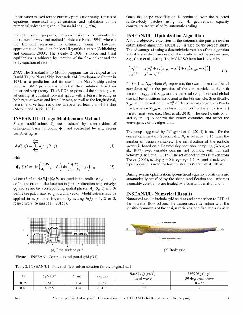
(a) Free-surface grid (b) Body grid
Figure 1. INSEAN - Computational panel grid (G1)
Table 2. INSEAN/UI - Potential flow solver solution for the original hull
Fr 𝐶F×10-3
𝛿 (m) 𝜏 (deg) 𝑅𝑀𝑆(𝑎R) (m/s
2),
head wave
𝑅𝑀𝑆(𝜙) (deg),
30 deg stern wave
0.25 2.643 0.134 0.052 - 0.477
0.41 6.068 0.424 -0.412 0.902 -
Diez Multi-objective Hydrodynamic Optimization of the DTMB 5415 for Resistance and Seakeeping 4
of the design optimization results obtained using six different
research spaces. Detailed results may be found in Serani et al.
(2015a).
Grid Studies and Comparison with EFD of the Potential Flow
Solvers. The computational domain (WARP) for the free-surface
is defined within one hull length upstream, three lengths
downstream and 1.5 lengths for the side (Fig. 1a). One panel grid
triplet (G1, G2, G3) is used, with a refinement ratio equal to 2,
and size equal to 11k, 5.5k and 2.8k, respectively. Figure 1b
shows the body grid (G1) for the DTMB 5415 under
consideration. The fluid condition are: 𝜌 = 998.5 kg/m3, 𝜐 =
1.09E-06 m2/s and 𝑔 = 9.8033 m/s
2.
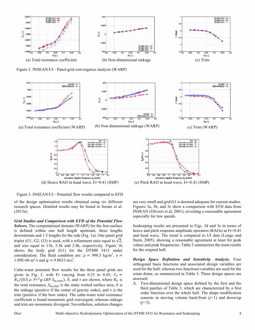
Calm-water potential flow results for the three panel grids are
given in Fig. 2, with Fr varying from 0.25 to 0.45; 𝐶F =𝑅F/(0.5𝜌𝐹𝑟
|𝑔𝐿𝐵𝑃𝑆�,�J�J), 𝛿, and 𝜏 are shown, where 𝑅F is
the total resistance, 𝑆�,�J�J is the static wetted surface area, 𝛿 is
the sinkage (positive if the center of gravity sinks), and 𝜏 is the
trim (positive if the bow sinks). The calm-water total resistance
coefficient is found monotonic grid convergent, whereas sinkage
and trim are monotonic divergent. Nevertheless, solution changes
are very small and grid G1 is deemed adequate for current studies.
Figures 3a, 3b, and 3c show a comparison with EFD data from
INSEAN (Olivieri et al, 2001), revealing a reasonable agreement
especially for low speeds.
Seakeeping results are presented in Figs. 3d and 3e in terms of
heave and pitch response amplitude operators (RAOs) at Fr=0.41
and head wave. The trend is compared to UI data (Longo and
Stern, 2005), showing a reasonable agreement at least for peak
values and peak frequencies. Table 2 summarizes the main results
for the original hull.
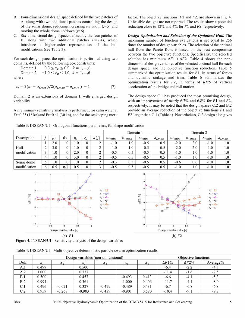
Design Space Definition and Sensitivity Analysis. Four
orthogonal basis functions and associated design variables are
used for the hull, whereas two functions/variables are used for the
sonar dome, as summarized in Table 3. Three design spaces are
assessed:
A. Two-dimensional design space defined by the first and the
third patches of Table 3, which are characterized by a first
order function over the whole hull. The shape modification
consists in moving volume back/front (j=1) and down/up
(j=3).
(a) Total resistance coefficient (b) Non-dimensional sinkage (c) Trim
Figure 2. INSEAN/UI - Panel-grid convergence analysis (WARP)
(a) Total resistance coefficient (WARP) (b) Non-dimensional sinkage (WARP) (c) Trim (WARP)
(d) Heave RAO in head wave, Fr=0.41 (SMP) (e) Pitch RAO in head wave, Fr=0.41 (SMP)
Figure 3. INSEAN/UI - Potential flow results compared to EFD
Diez Multi-objective Hydrodynamic Optimization of the DTMB 5415 for Resistance and Seakeeping 5
B. Four-dimensional design space defined by the two patches of
A, along with two additional patches controlling the design
of the sonar dome, reducing/increasing its width (j=5) and
moving the whole dome up/down (j=6).
C. Six-dimensional design space defined by the four patches of
B, along with two additional patches (j=2,4), which
introduce a higher-order representation of the hull
modifications (see Table 3).
For each design space, the optimization is performed using two
domains, defined by the following box constraints:
Domain 1. −0.5 ≤ 𝑥𝒌 ≤ 0.5, 𝑘 = 1,… ,6
Domain 2. −1.0 ≤ 𝑥𝒌 ≤ 1.0, 𝑘 = 1,… ,6
where
𝑥Z = 2(𝛼Z − 𝛼Z,�wT)/2(𝛼Z,��� − 𝛼Z,�wT) − 1 (7)
Domain 2 is an extensions of domain 1, with enlarged design
variability.
A preliminary sensitivity analysis is performed, for calm water at
Fr=0.25 (18 kn) and Fr=0.41 (30 kn), and for the seakeeping merit
factor. The objective functions, 𝐹1 and 𝐹2, are shown in Fig. 4.
Unfeasible designs are not reported. The results show a potential
reduction close to 12% and 4% for 𝐹1 and 𝐹2, respectively.
Design Optimization and Selection of the Optimized Hull. The
maximum number of function evaluations is set equal to 256
times the number of design variables. The selection of the optimal
hull from the Pareto front is based on the best compromise
between the two objective functions. Specifically, the selected
solution has minimum ∆𝐹1 + ∆𝐹2. Table 4 shows the non-
dimensional design variables of the selected optimal hull for each
design space, and the objective function reduction. Table 5
summarized the optimization results for 𝐹1, in terms of forces
and dynamic sinkage and trim. Table 6 summarizes the
optimization results for 𝐹2, in terms of 𝑅𝑀𝑆 of vertical
acceleration of the bridge and roll motion.
The design space C.1 has produced the most promising design,
with an improvement of nearly 6.7% and 6.8% for 𝐹1 and 𝐹2,
respectively. It may be noted that the design spaces C.2 and B.2
provide an average reduction of the objective functions 𝐹1 and
𝐹2 larger than C.1 (Table 4). Nevertheless, C.2 design also gives
Table 3. INSEAN/UI - Orthogonal functions parameters, for shape modification
Domain 1 Domain 2
Description 𝑗 𝑝Z 𝜙Z 𝑞Z 𝜒Z 𝑘(𝑗) 𝛼Z,�wT 𝛼Z,��� 𝑥Z,�wT 𝑥Z,��� 𝛼Z,�wT 𝛼Z,��� 𝑥Z,�wT 𝑥Z,���
Hull
modification
1 2.0 0 1.0 0 2 -1.0 1.0 -0.5 0.5 -2.0 2.0 -1.0 1.0
2 3.0 0 1.0 0 2 -1.0 1.0 -0.5 0.5 -2.0 2.0 -1.0 1.0
3 1.0 0 2.0 0 2 -0.5 0.5 -0.5 0.5 -1.0 1.0 -1.0 1.0
4 1.0 0 3.0 0 2 -0.5 0.5 -0.5 0.5 -1.0 1.0 -1.0 1.0
Sonar dome
modification
5 1.0 0 1.0 0 2 -0.3 0.3 -0.5 0.5 -0.6 0.6 -1.0 1.0
6 0.5 𝜋/2 0.5 0 3 -0.5 0.5 -0.5 0.5 -1.0 1.0 -1.0 1.0
(a) 𝐹1 (b) 𝐹2
Figure 4. INSEAN/UI - Sensitivity analysis of the design variables
Table 4. INSEAN/UI - Multi-objective deterministic particle swarm optimization results
Design variables (non-dimensional) Objective functions
DoE 𝑥H 𝑥| 𝑥L 𝑥� 𝑥� 𝑥� ∆𝐹1% ∆𝐹2% Average%
A.1 0.499 0.500 -6.4 -2.2 -4.3
A.2 1.000 0.737 -11.4 -1.6 -7.5
B.1 0.500 0.457 -0.493 0.413 -6.6 -4.1 -5.3
B.2 0.994 0.361 -1.000 0.406 -11.7 -4.1 -8.0
C.1 0.496 -0.021 0.327 -0.479 -0.489 0.431 -6.7 -6.8 -6.8
C.2 0.959 -0.268 -0.983 -0.489 -0.901 0.580 -10.4 -9.1 -9.8
Diez Multi-objective Hydrodynamic Optimization of the DTMB 5415 for Resistance and Seakeeping 6
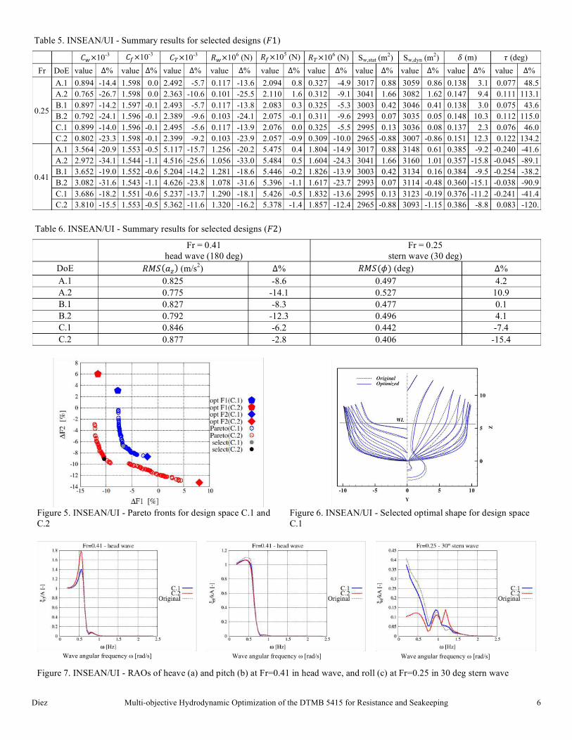
Table 5. INSEAN/UI - Summary results for selected designs (𝐹1)
𝐶�×10-3 𝐶�×10
-3 𝐶F×10
-3 𝑅�×10
6 (N) 𝑅�×10
5 (N) 𝑅F×10
6 (N) Sw,stat (m
2) Sw,dyn (m
2) 𝛿 (m) 𝜏 (deg)
Fr DoE value ∆% value ∆% value ∆% value ∆% value ∆% value ∆% value ∆% value ∆% value ∆% value ∆%
0.25
A.1 0.894 -14.4 1.598 0.0 2.492 -5.7 0.117 -13.6 2.094 0.8 0.327 -4.9 3017 0.88 3059 0.86 0.138 3.1 0.077 48.5
A.2 0.765 -26.7 1.598 0.0 2.363 -10.6 0.101 -25.5 2.110 1.6 0.312 -9.1 3041 1.66 3082 1.62 0.147 9.4 0.111 113.1
B.1 0.897 -14.2 1.597 -0.1 2.493 -5.7 0.117 -13.8 2.083 0.3 0.325 -5.3 3003 0.42 3046 0.41 0.138 3.0 0.075 43.6
B.2 0.792 -24.1 1.596 -0.1 2.389 -9.6 0.103 -24.1 2.075 -0.1 0.311 -9.6 2993 0.07 3035 0.05 0.148 10.3 0.112 115.0
C.1 0.899 -14.0 1.596 -0.1 2.495 -5.6 0.117 -13.9 2.076 0.0 0.325 -5.5 2995 0.13 3036 0.08 0.137 2.3 0.076 46.0
C.2 0.802 -23.3 1.598 -0.1 2.399 -9.2 0.103 -23.9 2.057 -0.9 0.309 -10.0 2965 -0.88 3007 -0.86 0.151 12.3 0.122 134.2
0.41
A.1 3.564 -20.9 1.553 -0.5 5.117 -15.7 1.256 -20.2 5.475 0.4 1.804 -14.9 3017 0.88 3148 0.61 0.385 -9.2 -0.240 -41.6
A.2 2.972 -34.1 1.544 -1.1 4.516 -25.6 1.056 -33.0 5.484 0.5 1.604 -24.3 3041 1.66 3160 1.01 0.357 -15.8 -0.045 -89.1
B.1 3.652 -19.0 1.552 -0.6 5.204 -14.2 1.281 -18.6 5.446 -0.2 1.826 -13.9 3003 0.42 3134 0.16 0.384 -9.5 -0.254 -38.2
B.2 3.082 -31.6 1.543 -1.1 4.626 -23.8 1.078 -31.6 5.396 -1.1 1.617 -23.7 2993 0.07 3114 -0.48 0.360 -15.1 -0.038 -90.9
C.1 3.686 -18.2 1.551 -0.6 5.237 -13.7 1.290 -18.1 5.426 -0.5 1.832 -13.6 2995 0.13 3123 -0.19 0.376 -11.2 -0.241 -41.4
C.2 3.810 -15.5 1.553 -0.5 5.362 -11.6 1.320 -16.2 5.378 -1.4 1.857 -12.4 2965 -0.88 3093 -1.15 0.386 -8.8 0.083 -120.
Table 6. INSEAN/UI - Summary results for selected designs (𝐹2)
Fr = 0.41
head wave (180 deg)
Fr = 0.25
stern wave (30 deg)
DoE 𝑅𝑀𝑆(𝑎R) (m/s2) ∆% 𝑅𝑀𝑆(𝜙) (deg) ∆%
A.1 0.825 -8.6 0.497 4.2
A.2 0.775 -14.1 0.527 10.9
B.1 0.827 -8.3 0.477 0.1
B.2 0.792 -12.3 0.496 4.1
C.1 0.846 -6.2 0.442 -7.4
C.2 0.877 -2.8 0.406 -15.4
Figure 5. INSEAN/UI - Pareto fronts for design space C.1 and
C.2
Figure 6. INSEAN/UI - Selected optimal shape for design space
C.1
(a) (b) (c)
Figure 7. INSEAN/UI - RAOs of heave (a) and pitch (b) at Fr=0.41 in head wave, and roll (c) at Fr=0.25 in 30 deg stern wave
Wave angular frequency ω [rad/s] Wave angular frequency ω [rad/s] Wave angular frequency ω [rad/s]
Diez Multi-objective Hydrodynamic Optimization of the DTMB 5415 for Resistance and Seakeeping 7
a significant penalization in terms of the heave motion response
(Fig. 7a), whereas B.2 design provides an RMS of the roll motion
worse than the original (Table 6). For these reasons, the C.1
optimal hull is selected for further investigation by RANSE.
Figure 5 shows the Pareto front and the selected solution for
design space C. The corresponding hull form (C.1) is shown in
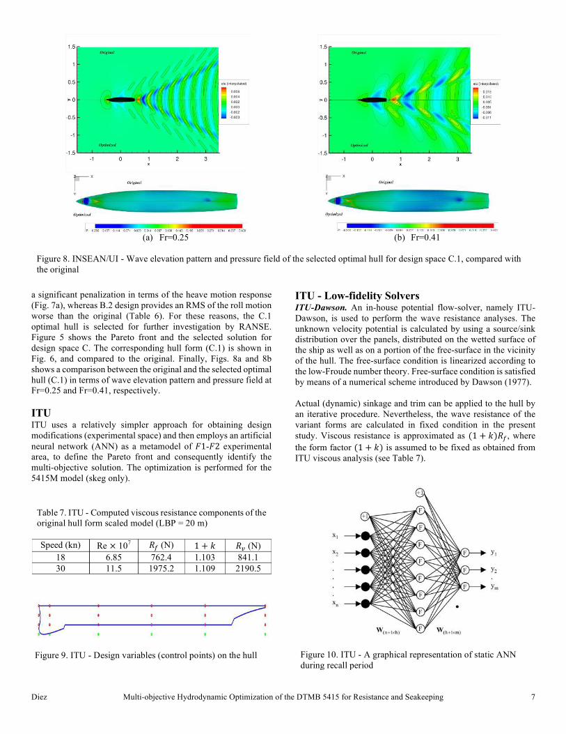
Fig. 6, and compared to the original. Finally, Figs. 8a and 8b
shows a comparison between the original and the selected optimal
hull (C.1) in terms of wave elevation pattern and pressure field at
Fr=0.25 and Fr=0.41, respectively.
ITU ITU uses a relatively simpler approach for obtaining design
modifications (experimental space) and then employs an artificial
neural network (ANN) as a metamodel of 𝐹1-𝐹2 experimental
area, to define the Pareto front and consequently identify the
multi-objective solution. The optimization is performed for the
5415M model (skeg only).
ITU - Low-fidelity Solvers ITU-Dawson. An in-house potential flow-solver, namely ITU-
Dawson, is used to perform the wave resistance analyses. The
unknown velocity potential is calculated by using a source/sink
distribution over the panels, distributed on the wetted surface of
the ship as well as on a portion of the free-surface in the vicinity
of the hull. The free-surface condition is linearized according to
the low-Froude number theory. Free-surface condition is satisfied
by means of a numerical scheme introduced by Dawson (1977).
Actual (dynamic) sinkage and trim can be applied to the hull by
an iterative procedure. Nevertheless, the wave resistance of the
variant forms are calculated in fixed condition in the present
study. Viscous resistance is approximated as (1 + 𝑘)𝑅�, where
the form factor (1 + 𝑘) is assumed to be fixed as obtained from
ITU viscous analysis (see Table 7).
(a) Fr=0.25 (b) Fr=0.41
Figure 8. INSEAN/UI - Wave elevation pattern and pressure field of the selected optimal hull for design space C.1, compared with
the original
Table 7. ITU - Computed viscous resistance components of the
original hull form scaled model (LBP = 20 m)
Speed (kn) Re × 107 𝑅� (N) 1 + 𝑘 𝑅] (N)
18 6.85 762.4 1.103 841.1
30 11.5 1975.2 1.109 2190.5
Figure 9. ITU - Design variables (control points) on the hull
Figure 10. ITU - A graphical representation of static ANN
during recall period

Diez Multi-objective Hydrodynamic Optimization of the DTMB 5415 for Resistance and Seakeeping 8
ITU-SHIPMO. Usual strip theory is employed to obtain vertical
acceleration at the bridge at 30 kn in head seas and roll amplitude
in 30 deg stern waves at 18 kn. The two dimensional added mass
and damping coefficients are predicted by using the Frank Close-
Fit method which is a module in the in-house code ITU-SHIPMO.
ITU - Design Modification Method On the one hand, hull-form generation from a parent shape, by
variation of basic hull parameters, may not be fruitful because the
derived hull forms inherit the characteristics of the parent hull.
On the other hand, varying the hull surface points directly may
generate fairing issues and generally one has to deal with a very
large number of design variables. In order to overcome these
difficulties, a simpler approach is adopted, which uses limited
number of control points (see Fig. 9) at which randomly
distributed relaxation coefficients (between 0.95 and 1.05 in this
study) are assigned to modify the hull surface. This means that a
3D matrix is formed with limited number of rows (𝒙(𝒊)) and
columns (𝒛(𝒊)), and corresponding to this pair of coordinates there
is a randomly assigned value of relaxation coefficients 𝑪𝒓. Akima’s (1978) surface generation method, from a set of
scattered points, is used to define the surface related to these
coefficients; that is, by using 𝑥 and 𝑧 coordinates of a particular
point:
𝒚(𝒎) = 𝒚(𝒊) · 𝑪𝒓(𝒙(𝒊), 𝒛(𝒊)) (8)
where 𝒚(𝒎) is the modified value of the initial offset of 𝒚(𝒊). Furthermore, to have a finer mesh, the relaxation coefficients for
other intermediate (interpolation) points are obtained by
interpolation using the coefficients defined (assigned) at the
control points.
ITU - Optimization Algorithm A database of 250 modified hull forms is obtained by means of
the design modification method described above. Static artificial
neural networks have the capability of storing data during the
learning process and then reproducing these data during the recall
process. Danisman et al. (2002), Danisman (2014) presented this
ANN ability for hull form optimization purposes.
ANN simply establish a functional relationship between ℝT and
ℝ�, assumed to be input and output data spaces of dimensions 𝑛
and 𝑚, respectively. Figure 10 shows the input and output
vectors, respectively, as 𝑿 = (𝑥H, 𝑥|, … , 𝑥T) and Y =(𝑦H, 𝑦|, … , 𝑦T). The numerical flow solver provides a set of
output values, such as wave resistance (𝑅�), in response to a set
of input values (control variables, 𝑥H, 𝑥|, … , 𝑥T). After a
successful training, the ANN can easily and reliably replace the
Figure 11. ITU - Panel distribution over the hull and its free-
surface vicinity
Figure 12. ITU - Predicted and measured (circles) heave
RAOs in head seas (180 deg)
0.3 0.4 0.5 0.6 0.7 0.8 0.9 1.0 1.1 1.2
Wave Frequency
0.0
0.1
0.2
0.3
0.4
0.5
0.6
0.7
0.8
0.9
1.0
1.1
1.2
1.3
1.4
HeaveAmplitude/WaveAmplitude
V= 18 Knots
V= 30 Knots
Table 8. ITU - First 10 hull variants in terms of the regression coefficients for each control point on the hull (from the database used
in ANN training process)
𝑥H 𝑥| 𝑥L 𝑥� 𝑥� 𝑥� 𝑥¢ 𝑥I 𝑥£ 𝑥HM 𝑥HH 𝑥H| 𝐹¤¥�{wT¦\�
1.000 1.000 1.000 1.000 1.000 1.000 1.000 1.000 1.000 1.000 1.000 1.000 1.000
0.952 1.003 1.093 0.938 1.085 1.091 0.981 0.937 0.953 1.026 1.008 1.013 1.050
1.003 1.074 1.001 0.988 1.016 0.983 1.048 0.951 0.922 1.097 1.071 0.986 0.952
1.028 0.953 1.070 0.957 0.989 0.949 0.950 0.905 0.974 0.920 0.938 0.977 1.030
1.083 0.910 1.009 1.011 0.996 0.986 1.005 1.063 1.033 1.052 1.095 1.054 0.990
0.942 1.053 0.952 0.927 0.919 0.910 0.933 0.920 1.084 0.977 1.001 0.949 0.908
1.031 1.097 1.066 1.093 0.941 0.983 0.919 1.021 0.919 1.003 1.076 0.962 1.070
1.052 0.956 1.090 0.970 1.022 0.908 1.092 1.086 0.906 0.912 0.920 0.920 1.050
0.956 1.035 0.999 0.920 0.993 1.085 1.040 0.990 0.961 1.001 0.903 1.064 0.935
0.936 0.957 0.917 1.065 1.067 1.091 1.038 1.003 1.000 1.074 1.027 0.952 0.975
Diez Multi-objective Hydrodynamic Optimization of the DTMB 5415 for Resistance and Seakeeping 9
numerical flow solver. In order to determine the Pareto front out
of the experimental area, a simpler and a basic approach is
considered where the combined (or aggregate) objective function
is expressed as
𝐹¤¥�{wT¦\� = 𝑤×𝐹1 + (1 − 𝑤)×𝐹2 (9)
where 𝑤 = 0, 0.1, … ,0.9, 1.0 is employed as a weighting factor.
The selected optimization algorithm is based on sequential
quadratic programming (SQP) within Matlab optimization
toolbox, since it is very suitable for constraint optimization
problems whose design variables include upper and lower
bounds. Schittkowski (1985) showed the success of this
algorithm in many aspects such as accuracy, efficiency and
number of successful solutions over a large number of test
problems.
ITU - Numerical Results Computational Setup and Results for Resistance and
Seakeeping. Grid convergence (or panel-grid sensitivity analysis)
is not shown for the present case, since grid studies have been
performed on the code ITU-Dawson for similar hull forms.
Accordingly, about 1300 panels over the hull surface (demi-hull)
and 1600 panels over the free-surface (half symmetric plane) are
used. Dimensions of the panelled free-surface are: 1.0 LBP
upstream, 1.5 LBP downstream and 0.85 LBP sidewise.
Preliminary benchmark tests, with the discretization model given
in Fig. 11, show that the code satisfactorily computes wave
resistance of the hull forms in consideration. As to the viscous
resistance, only the changes in the wetted surface area of the
variant hull forms are reflected in the viscous resistance through
the frictional resistance, 𝑅�.
As a representative output of the present code, the predicted and
measured heave RAOs for model 5415M at 18 kn and 30 kn are
shown in Fig. 12.
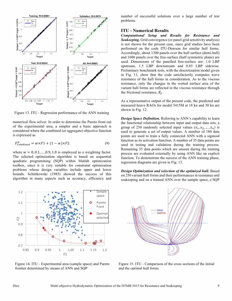
Design Space Definition. Referring to ANN’s capability to learn
the functional relationship between input and output data sets, a
group of 250 randomly selected input values (𝑥H, 𝑥|, … , 𝑥T) is
used to generate a set of output values. A number of 180 data
points are used to train a fully connected ANN with a sigmoid
function as its activation function. A number of 35 data points are
used in testing and validation during the training process.
Remaining 35 data points which are unseen during the training
process are evaluated externally by using ANN like an explicit
function. To demonstrate the success of the ANN training phase,
regression diagrams are given in Fig. 13.
Design Optimization and selection of the optimized hull. Based
on 250 variant hull forms and their performances in resistance and
seakeeping and on a trained ANN over the sample space, a SQP
Figure 13. ITU - Regression performance of the ANN training
Figure 14. ITU - Experimental area (sample space) and Pareto
frontier determined by means of ANN and SQP
Figure 15. ITU - Comparison of the cross sections of the initial
and the optimal hull forms
0.7
0.8
0.9
1
1.1
1.2
0.85 0.9 0.95 1 1.05 1.1 1.15 1.2
F2
F1
Sample
space
Pareto
Front
Optimal
selected

Diez Multi-objective Hydrodynamic Optimization of the DTMB 5415 for Resistance and Seakeeping 10
process is carried out to optimize the prescribed aggregate
objective function with weighting factors 𝑤. The optimal forms
for each weighting factor (𝑤) are investigated by considering
𝐹¤¥�{wT¦\� in the ANN training process (see Table 8). The SQP
application on the metamodel provided by ANN gives an optimal
point, which is expected to be part of the overall Pareto front. An
optimal point is selected on the Pareto front according to the
changes in the Pareto curve, in order to give favorable results for
both 𝐹1 and 𝐹2. Figure 14 shows 𝐹1 vs 𝐹2 values of the variant
hull forms, the approximated Pareto front and the optimal design.
The comparison of the cross sections of the initial and the optimal
hull forms can be observed in Fig. 15. Wave deformations of the
initial and the optimal hull forms, for 18 and 30 kn, are presented
in Fig. 16, which points out the success of the selected optimal
hull. The contour plot of the wave patterns of the initial and the
optimal hull forms can be compared in Fig. 17. The summary of
the seakeeping performance of the present multi-objective
process is given in Table 9 and the final overall performance in
terms of 𝐹1 and 𝐹2 is summarized in Table 10.
NTUA NTUA integrates the parametric modelling and optimization
algorithm of the CAESES/FRIENDSHIP-Framework (FFW)
with two low-fidelity solvers for calm water and seakeeping
performances (Kring and Sclavounos, 1995; Sclavounos, 1996).
Optimization results are shown for the 5415M model (skeg only).
NTUA - Low-fidelity Solvers The hydrodynamic performance of the initial hull form and its
variants is evaluated via the commercial SWAN2 2002 code for
the calm water and the custom-made code SPP-86 for the rough
water.
Figure 16. ITU - Wave deformations of the initial and the optimal
hull at 18 and 30 kn
Figure 17. ITU - Contour plot of the wave patterns of the initial
and the optimal hull forms (30 kn)
Table 9. ITU - Comparative seakeeping performances Table 10. ITU - Performance of the solution out of the
multi-objective problem
Hull
Fr = 0.41
head wave
Fr = 0.25, 30 deg
stern wave
𝑅𝑀𝑆(𝑎R) (m/s2) 𝑅𝑀𝑆(𝜙) (deg) Hull 𝐹1 𝐹2
Original 0.806 2.321 Original 1.000 1.000
Pareto optimum 0.792 2.015 Pareto optimum 0.928 0.865
∆% -1.9 -13.2 ∆% -7.2 -13.5
(a) Free-surface
(b) Body surface
Figure 18. NTUA - Spline sheet on the computational grid
Diez Multi-objective Hydrodynamic Optimization of the DTMB 5415 for Resistance and Seakeeping 11
SWAN2 2002. The Ship Wave ANalysis is a software package
for the hydrodynamics analysis developed at MIT (Kring and
Sclavounos, 1995). SWAN2 2002 distributes quadrilateral panels
over the ship hull and the free surface to derive numerically the
steady and unsteady free-surface potential flow around ships,
using a three-dimensional Rankine Panel Method in the time
domain. Only the calm water results are used in the present study.
A batch file is used to integrate SWAN2 with the CAESES/FFW.
Additional calculations in calm water have been carried out via a
potential flow code developed in-house at Laboratory for Ship
and Marine Hydrodynamics (LSMH) of NTUA (Tzabiras, 2008).
The code solves the non-linear potential flow around the ship, by
calculating iteratively the free surface, while both the dynamic
and kinematic conditions are satisfied on it. The free surface and
the solid boundary are covered by quadrilateral elements. The
distribution of panels varies, being denser near geometrical
discontinuities and areas of expected high pressures. The Laplace
equation is solved according to the classical Hess and Smith
(1968) method. An iterative Lagrangian procedure is adopted to
cope with the non-linear problem, in conjunction with an Eulerian
solution of the vertical momentum equation. Table 12 has been
derived on the basis of this method.
SPP-86. The seakeeping qualities of the parent and the variant
hull forms are calculated by the SPP-86 code, developed at
LSMH of NTUA to implement the Salvensen, Tuck and Faltinsen
(1970) strip theory. The code distributes Kelvin sources along the
wetted part of each ship section following Frank (1967) method.
The estimated dynamic responses encompasses vertical and
lateral motions, velocities and accelerations and velocities at
specific points for a variety of wave frequencies and heading
angles.
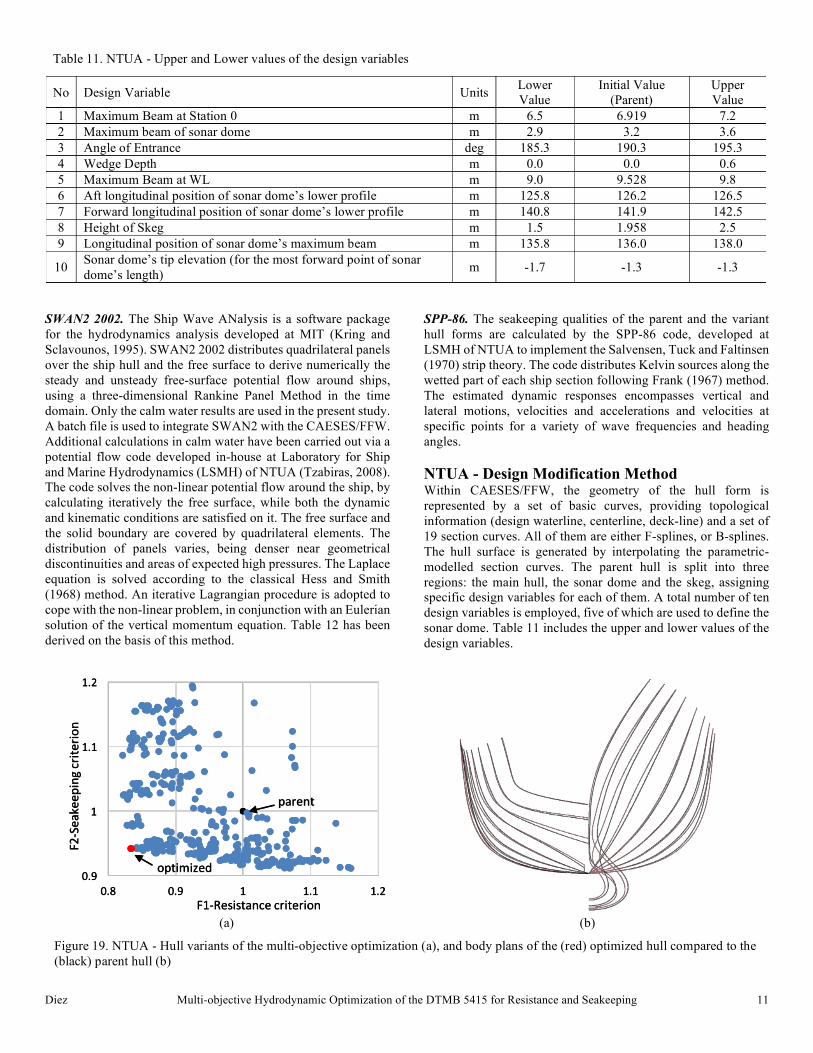
NTUA - Design Modification Method Within CAESES/FFW, the geometry of the hull form is
represented by a set of basic curves, providing topological
information (design waterline, centerline, deck-line) and a set of
19 section curves. All of them are either F-splines, or B-splines.
The hull surface is generated by interpolating the parametric-
modelled section curves. The parent hull is split into three
regions: the main hull, the sonar dome and the skeg, assigning
specific design variables for each of them. A total number of ten
design variables is employed, five of which are used to define the
sonar dome. Table 11 includes the upper and lower values of the
design variables.
Table 11. NTUA - Upper and Lower values of the design variables
No Design Variable Units Lower
Value
Initial Value
(Parent)
Upper
Value
1 Maximum Beam at Station 0 m 6.5 6.919 7.2
2 Maximum beam of sonar dome m 2.9 3.2 3.6
3 Angle of Entrance deg 185.3 190.3 195.3
4 Wedge Depth m 0.0 0.0 0.6
5 Maximum Beam at WL m 9.0 9.528 9.8
6 Aft longitudinal position of sonar dome’s lower profile m 125.8 126.2 126.5
7 Forward longitudinal position of sonar dome’s lower profile m 140.8 141.9 142.5
8 Height of Skeg m 1.5 1.958 2.5
9 Longitudinal position of sonar dome’s maximum beam m 135.8 136.0 138.0
10 Sonar dome’s tip elevation (for the most forward point of sonar
dome’s length) m -1.7 -1.3 -1.3
(a) (b)
Figure 19. NTUA - Hull variants of the multi-objective optimization (a), and body plans of the (red) optimized hull compared to the
(black) parent hull (b)
0.9
1
1.1
1.2
0.8 0.9 1 1.1 1.2
F2-Seakeepingcriterion
F1-Resistancecriterion
parent
optimized
Diez Multi-objective Hydrodynamic Optimization of the DTMB 5415 for Resistance and Seakeeping 12
The variation of the hull geometries is made by simply giving an
upper and a lower value of the chosen design variables, to the
CAESES/FFW environment. The aforementioned boundaries are
selected after inspection that they refer to smooth hull shapes. In
addition, they comply with the DTMB 5415 geometrical
constraints.
NTUA - Optimization Algorithm The NSGA II (Non-Dominated Sorting Genetic Algorithm II;
Deb, 2002) has been selected for the optimization process. The
procedure of this algorithm is described below:
1. A number of variant geometries is generated.
2. An equal number of off-springs is formed.
3. The total number of parents and offspring is sorted to levels
according to non-domination.
4. The geometries of each level are ranked with respect to their
crowded distance of each solution in the population.
5. A new generation is being produced with a population
number equal to the initial one.
6. Steps 2 to 5 are repeated.
The diversity among non-dominated solutions is introduced by
using the crowding comparison procedure where for two different
solutions 𝑝 and 𝑞, 𝑝 dominates (𝑝 < 𝑞) if the following is
attained:
𝑓Z 𝑥H ≤ 𝑓Z 𝑥| , ∀𝑗 ∈ 1, … , 𝑛
𝑓5 𝑥H < 𝑓5 𝑥| , ∀𝑘 ∈ 1, … , 𝑛 (10)
where 𝑥H and 𝑥| represent the design variables for 𝑝 and 𝑞
geometries respectively.
Table 12. NTUA - Comparative seakeeping performances of
the hulls
Hull
Fr = 0.41
head wave
Fr = 0.25, 30 deg
stern wave
𝑅𝑀𝑆(𝑎R) (m/s2) 𝑅𝑀𝑆(𝜙) (deg)
Original 0.982 0.874
Pareto optimum 0.990 0.766
∆% 0.81 -12.3
Table 13. NTUA - Performance of the solution out of the
multi-objective problem
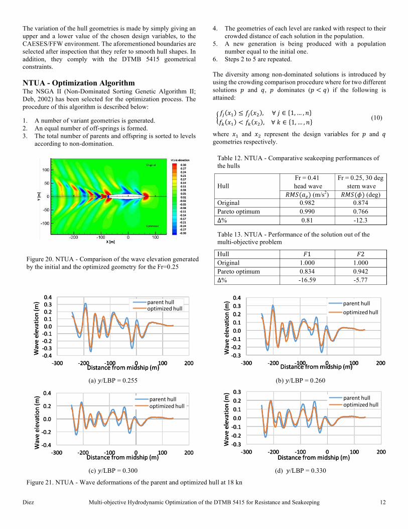
Figure 20. NTUA - Comparison of the wave elevation generated
by the initial and the optimized geometry for the Fr=0.25
Hull 𝐹1 𝐹2
Original 1.000 1.000
Pareto optimum 0.834 0.942
∆% -16.59 -5.77
(a) 𝑦/LBP = 0.255
(b) 𝑦/LBP = 0.260
(c) 𝑦/LBP = 0.300
(d) 𝑦/LBP = 0.330
Figure 21. NTUA - Wave deformations of the parent and optimized hull at 18 kn
-0.4
-0.3
-0.2
-0.1
0.0
0.1
0.2
0.3
0.4
-300 -200 -100 0 100 200
Waveelevation(m)
Distancefrommidship(m)
parenthulloptimizedhull
-0.3
-0.2
-0.1
0.0
0.1
0.2
0.3
0.4
-300 -200 -100 0 100 200
Waveelevation(m)
Distancefrommidship(m)
parenthull
optimizedhull
-0.4
-0.2
0.0
0.2
0.4
-300 -200 -100 0 100 200
Waveelevation(m)
Distancefrommidship(m)
parenthull
optimizedhull
-0.3
-0.2
-0.1
0.0
0.1
0.2
0.3
-300 -200 -100 0 100 200
Waveelevation(m)
Distancefrommidship(m)
parenthull
optimizedhull
Diez Multi-objective Hydrodynamic Optimization of the DTMB 5415 for Resistance and Seakeeping 13
More information is provided by Deb (2002). A number of 25
generations and a population size of 16 are selected, whereas the
mutation and the crossover probability are equal to 0.01 and 0.9,
respectively.
NTUA - Numerical Results Panel mesh generation. The panel mesh generation of the free-
surface and the body surface of the hull is an internal routine of
SWAN2 2002. The spline sheet of the body surface is defined by
45 nodes in a direction parallel to the 𝑥-axis, corresponding to a
number of 44 panels in the 𝑥 direction, and by 13 nodes
athwarships. The domain of the free surface is defined by 0.5 LBP
upstream, 1.5 LBP downstream and 1 LBP along the transverse
distance. Figure 18 presents the spline sheet of the free-surface
(a) and the body (b), respectively.
Design Optimization and selection of the optimized hull. The
solutions with respect to both the resistance (𝐹1) and the
seakeeping (𝐹2) criterion, calculated in SWAN2, are shown in
Fig. 19a. The solutions concern the variation of 400 hull forms
produced by NGSA-II, The selected optimal (red) and the parent
hull (black) are also shown in Fig. 19a. Figure 19b depicts a
comparison between the body plans of the parent and the
optimized hull. Figure 20 shows the comparison of the contour
plot of the wave elevation between the initial and the optimized
hull at 18 kn.
Even thought the 𝐹1 objective function concerns the total
resistance (including the wave resistance computed by the
potential flow code), a comparison between the height of waves
generated in specific longitudinal cuts along the ship for the
parent and the optimized hull has been made. Figure 21 presents
the profile of the waves generated by the initial hull, for 𝑦/LBP =
(a) 0.225, (b) 0.260, (c) 0.300, (d) 0.330.
The origin of the coordinate system is assumed amidships and on
the free surface. Table 12 summarized summarized the
optimization results for 𝐹2 in terms of 𝑅𝑀𝑆 vertical acceleration
at the bridge and roll motion. 𝐹1 and 𝐹2 objectives improvements
are summarized in Table 13.
ECN The role of ECN/CNRS is to verify the performances of the
optimized hulls by high-fidelity computations.
ECN - High-fidelity Solver ISIS-CFD is a flow solver for the incompressible unsteady
Reynolds-averaged Navier-Stokes equation (RANSE), available
as a part of the FINETM/Marine computing suite. The solver is
fully implicit, based on the finite volume method to build the
spatial discretization of the transport equations. Surface and
volume integrals are evaluated according to second-order
accurate approximations and the unstructured discretization is
face-based. Time derivatives are evaluated using three-level
Euler second-order accurate approximations. While all unknown
state variables are cell-centered, the systems of equations used in
the implicit time stepping procedure are constructed face by face.
Fluxes are computed in a loop over the faces and the contribution
of each face is then added to the two cells next to the face. This
technique poses no specific requirements on the topology of the
cells. Therefore, the grids can be completely unstructured; cells
with an arbitrary number of arbitrarily-shaped faces are accepted.
Pressure-velocity coupling is obtained through a Rhie and Chow
(1983) SIMPLE type method: in each time step, the velocity
updates come from the momentum equations and the pressure is
given by the mass conservation law, transformed into a pressure
equation. In the case of turbulent flows, transport equations for
the variables in the turbulence model are added to the
discretization. Free-surface flow is simulated with a multi-phase
flow approach: the water surface is captured with a conservation
equation for the volume fraction of water, discretized with
specific compressive discretization schemes (Queutey and
Visonneau, 2007).
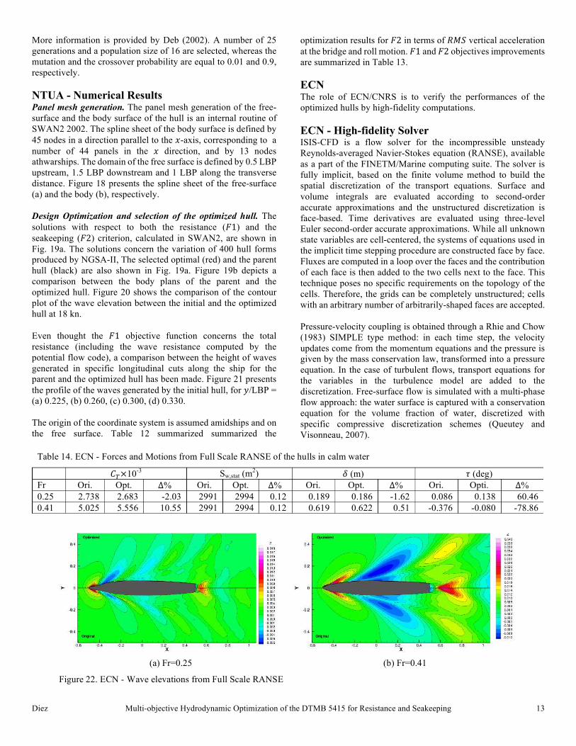
Table 14. ECN - Forces and Motions from Full Scale RANSE of the hulls in calm water
𝐶F×10-3 Sw,stat (m
2) 𝛿 (m) 𝜏 (deg)
Fr Ori. Opt. ∆% Ori. Opt. ∆% Ori. Opt. ∆% Ori. Opti. ∆%
0.25 2.738 2.683 -2.03 2991 2994 0.12 0.189 0.186 -1.62 0.086 0.138 60.46
0.41 5.025 5.556 10.55 2991 2994 0.12 0.619 0.622 0.51 -0.376 -0.080 -78.86
(a) Fr=0.25 (b) Fr=0.41
Figure 22. ECN - Wave elevations from Full Scale RANSE
Diez Multi-objective Hydrodynamic Optimization of the DTMB 5415 for Resistance and Seakeeping 14
The method features sophisticated turbulence models: apart from
classical one equation and two-equation 𝑘 − 𝜀 and 𝑘 − 𝜔 models
(Menter, 1993), the anisotropic two-equation Explicit Algebraic
Reynolds Stress Model (EARSM) (Deng et al., 2006), as well as
hybrid RANSE-LES (Large-Eddy Simulation) (Guilmineau et al.,
2013). The technique included for the 6 DOF simulation of ship
motion is described by Leroyer and Visonneau (2005). Time-
integration of Newton's laws for the ship motion is combined with
analytical weighted or elastic analogy grid deformation to adapt
the fluid mesh to the moving ship.
Parallelism is based on domain decomposition. The grid is
divided into different partitions, these partitions contain the cells.
The interface faces on the boundaries between the partitions are
shared between the partitions; information on these faces is
exchanged with the MPI (Message Passing Interface) protocol.
This method works with the sliding grid approach and the
different sub-domains can be distributed arbitrarily over the
processors.
ECN - Numerical Results ECN/CNRS has verified the optimized geometry by INSEAN/UI
(Fig. 6). At the current stage, the verification includes only calm
water performance of the original and optimized C.1 geometries,
in full scale, and at moderate and high Froude numbers (Fr=0.25
and 0.41). The hull performances are computed in a free to sink
and trim condition by combining the free-surface and moving
mesh capabilities with a rigid body motion solver for the
flow/motion interaction.
The numerical settings and physical modelling are those of
RANSE simulation with a wall function approach with the SST
𝑘 − 𝜔 turbulence model. The target 𝑦x value on the walls is 300,
suited for Reynolds number Re=1.2x10⁹ for Fr=0.25, and
Re=2x10⁹ for Fr=0.41. For symmetry consideration, only 𝑦-
symmetric boat is considered. The mesh is generated with the
hexahedral HEXPRESSTM mesh generator with anisotropic grid
refinement close to water plane at rest in order to resolve the free-
surface deformations for interface capturing method (both air and
water solved). A similar grid is used for the two geometries with
1.3M cells and about 80K cells on the bare hull. The vertical
resolution of the free-surface is about 15 cm corresponding to
0.001 LBP. The computation starts with the ship in even keel
position and in prescribed draft of 0.0433 LBP.
Table 14 summarizes the normalized computed forces and
motions to reach the final equilibrium state. Concerning the EFD
data for the original geometry in model scale (from IIHR; Longo
and Stern, 2005), only the trim angle and the sink can be
compared with the CFD values, under the hypothesis that the
scale effect is weak on these quantities. EFD predicts a trim angle
of 0.085 deg at Fr=0.25 and -0.421 deg at Fr=0.41 and the
measured sink value is 0.189 at Fr=0.25 and 0.619 at Fr=0.41.
Under the aforementioned hypothesis, this is in agreement with
the CFD values from Table 14. It may be noted that the computed
trim is close to the experiments for both RANSE and potential
flow; for the computed sinkage, the agreement appears correct
with RANSE, whereas it is under predicted at both speeds with
the potential flow (see Table 3).
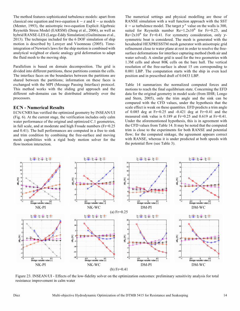
NK-PI NK-WC DM-PI DM-WC
(a) Fr=0.25
NK-PI NK-WC DM-PI DM-WC
(b) Fr=0.41
Figure 23. INSEAN/UI - Effects of the low-fidelity solver on the optimization outcomes: preliminary sensitivity analysis for total
resistance improvement in calm water
Diez Multi-objective Hydrodynamic Optimization of the DTMB 5415 for Resistance and Seakeeping 15
Concerning the forces, it results that with RANSE the resistance
coefficient is decreased by 2% at Fr=0.25, and is increased by
10% at Fr=0.41. The improvement for 𝐹1, as calculated by
RANSE, reduces significantly, providing a final weighted
resistance reduction by 0.2%. Figure 22 shows a comparison of
the wave elevation patterns for the original and the optimized
geometry at Fr=0.25 (a) and Fr=0.41 (b), respectively. At the
lower Froude number, the bow waves are similar although less
pronounced with the optimized geometry. Two other effects can
explain the predicted reduced resistance of the optimized hull: a
more pronounced wave through close to the bow and a reduced
level of the stern wave. At Fr=0.41 a significant breaking bow
wave is detected on the optimized hull with an increased wave
through at mid-ship.
CONCLUSIONS AND FUTURE WORK The paper presented a multi-objective hull form optimization of
the DTMB 5415 (specifically the MARIN variant 5415M, with
skeg only), performed by three different research team
(INSEAN/UI, ITU, and NTUA) within the NATO RTO Task
Group AVT-204 to the aim of “Assess the Ability to Optimize
Hull Forms of Sea Vehicles for Best Performance in a Sea
Environment.” Low-fidelity solvers, such as potential flow/strip
theory methods, have been used to assess and improve the calm
water (𝐹1) and the seakeeping (𝐹2) performances at two speeds
(Fr=0.25 and Fr=0.41) and two heading (head and stern wave) at
sea state 5, respectively. The results have been partially verified
by ECN/CNRS by high-fidelity simulations using a RANSE
solver.
Overall, optimization achievements by low-fidelity solvers have
been found significant, with an average improvement for calm-
water resistance and seakeeping performances of 10 and 9%
respectively. Moreover, the most promising designs have shown
up to 16% improvement for the calm-water resistance and 14%
for the seakeeping merit factor. The design-space size ranged
from two to twelve and the optimized designs show a quite large
variability and different characteristic (Figs. 6, 15, and 19), which
will be investigated and compared in detail by high-fidelity
solvers in future work.
INSEAN/UI has defined six design spaces with dimensionality
ranging from two to six, using a linear expansion of orthogonal
basis functions for the modification of the DTMB 5415 bare hull.
The optimization is performed by a multi-objective extension of
the deterministic particle swarm optimization algorithm. The
most promising design is identified, showing an improvement of
nearly 6.7% and 6.8% for 𝐹1 and 𝐹2 respectively.
ITU has produced 250 hull form variants of the 5415M using
Akima’s surface generation, with randomly distributed relaxation
coefficients at control points over the body surface. The
optimization procedure combines an artificial neural network
with a sequential quadratic programming algorithm, which is fed
with aggregate objective functions. The selected optimal hull has
achieved an improvement of 7.2% and 13.5% for 𝐹1 and 𝐹2,
respectively.
NTUA has used the parametric modelling of the
CAESES/FRIENDSHIP-Framework for the design modification
of the 5415M, representing the hull form by a set of basic curves,
providing topological information, and defining a set of 19
sections. The hull surface is parametrized by ten design variables.
The NSGA II code is used for the optimization procedure. The
selected optimal hull has reached an improvement of nearly
23.4% and 5.8% for 𝐹1 and 𝐹2, respectively.
ECN/CNRS has verified the parent and the INSEAN/UI optimal
hull for the calm water performances, using an in-house high-
fidelity solver (ISIS-CFD). The CFD results have shown a
resistance reduction of 2% at Fr=0.25 and an increment of 10%
at Fr=0.41, proving an overall 0.2% reduction for 𝐹1. Comparing
to ISIS-CFD, the calm water resistance evaluated by the potential
flow code WARP shows a -3.6 and -7.1% error for the original
and optimized hull respectively, at Fr=0.25; the error at Fr=0.41
is 21 and -5.8% for original and optimized hull, respectively. This
has motivated further studies on the impact of the low-fidelity
solver on the design optimization outcomes.
Further investigations on the effects of potential flow
formulation/linearization on the multi-objective optimization of
the DTMB 5145 are in progress by INSEAN/UI. A preliminary
sensitivity analysis of the design variables for the calm water
resistance at Fr=0.25 and 0.41 is shown in Fig. 23, where
Neumann-Kelvin (NK) and double model or Dawson (DM)
linearization are combined with a standard pressure integral (PI)
and the transversal wave cut (WC) method for the wave resistance
evaluation. The trend of some of the variables, such as x1, is very
sensitive to the formulation used, which may lead to inaccurate
design optimization solutions. The identification of the proper
trend of the design variables remains a critical issue for low
fidelity solvers, especially when large shape modifications are
produced. This suggests the use of high-fidelity solvers combined
with metamodels, in order to increase the accuracy of the design
optimization while keeping the computational cost affordable.
Future work includes RANSE simulations by ECN/CNRS of ITU
and NTUA optimal designs, as well as the assessment of the
maneuvering performance (steady turn) for parent and most
promising optimized hulls. In addition, a high-fidelity RANSE
SBDO, based on sequential multi-criterion adaptive sampling and
dynamic radial basis function (Diez et al., 2015) will be
performed by INSEAN/UI. TUHH will address optimal
propulsion studies for selected hull forms. The final assessment
of the results will be used to draw the final conclusions for the
current optimization exercise, and provide recommendations for
effective ship optimization procedures.
Beyond the scopes of the current activities, the design
optimization of the DTMB 5415 will be extended to stochastic
environment and operations by UI and INSEAN, for reduced
resistance/power in wave and increased ship operability. The ship
performances will be addressed by uncertainty quantification
methods for stochastic sea state, speed, and heading and will be
optimized by metamodels and multi-objective particle swarm.
The results will be compared to the current studies, which
represent the deterministic baseline for the future stochastic
optimization of the DTMB 5415.

Diez Multi-objective Hydrodynamic Optimization of the DTMB 5415 for Resistance and Seakeeping 16
ACKNOWLEDGMENTS The work has been performed in collaboration with NATO RTO
Task Group AVT-204 “Assess the Ability to Optimize Hull
Forms of Sea Vehicles for Best Performance in a Sea
Environment.”
CNR-INSEAN and University of Iowa teams are grateful to Dr
Woei-Min Lin and Dr Ki-Han Kim of the US Navy Office of
Naval Research, for their support through NICOP grant N62909-
11-1-7011 and grant N00014-14-1-0195. INSEAN team is also
grateful to the Italian Flagship Project RITMARE, coordinated
by the Italian National Research Council and funded by the Italian
Ministry of Education.
ECN/CNRS team gratefully acknowledge GENCI (Grand
Equipement National de Calcul Intensif) for the HPC resources
under Grant No 2014-21308.
REFERENCES 1. Akima H., “A Method of Bivariate Interpolation and Smooth
Surface Fitting for Irregularly Distributed Data Points.”
ACM Transactions on Mathematical Software 4 (1978): 148-
159.
2. Bassanini P., Bulgarelli U., Campana E.F., Lalli F., “The
wave resistance problem in a boundary integral
formulation.” Surv. Math. Ind. 4 (1994): 151-194.
3. Chen X., Diez M., Kandasamy M., Zhang Z., Campana E.F.,
Stern F., “High-fidelity global optimization of shape design
by dimensionality reduction, metamodels and deterministic
particle swarm.” Engineering Optimization 47(4)
(2015):473-494.
4. Danisman D.B., Mesbahi E., Atlar M., Goren O., “A New
Hull Form Optimisation Technique For Minimum Wave
Resistance.” 10th IMAM Congress, Crete, Greece, (13-17
May 2002).
5. Danisman D.B., “Reduction of demi-hull wave interference
resistance in fast displacement catamarans utilizing an
optimized centerbulb concept.” Ocean Engıneering 91
(2014):227–234.
6. Dawson C.W., “A Practical Computer Method For Solving
Ship-Wave Problems.” 2nd Int. Conf. Numerical Ship
Hydrodynamics, Berkeley (1977): 30-38.
7. Deb K., “A fast and elitist multiobjective genetic algorithm:
NSGA-II.” Evolutionary Computation, IEEE Transactions
6(2) (2002): 182-197.
8. Deng G., Queutey P., Visonneau M., “Three-dimensional
flow computation with Reynolds stress and algebraic stress
models.” in Rodi W., Mulas M. eds, Engineering Turbulence
Modelling and Experiments 6 (2006): 389-398.
9. Diez M., Peri D., “Robust optimization for ship conceptual
design.” Ocean Engineering 37(11) (2010): 966-977.
10. Diez M., Volpi S., Serani A., Stern F., Campana E.F.,
“Simulation-based Design Optimization by Sequential
Multi-criterion Adaptive Sampling and Dynamic Radial
Basis Functions.” In Proc. EUROGEN 2015 - International
Conference on Evolutionary and Deterministic Methods for
Design, Optimization and Control with Applications to
Industrial and Societal Problems, University of Strathclyde,
Glasgow, UK, (14-16 Sept. 2015).
11. Frank W., “Oscillation of Cylinders in or Below the Free
Surface of Deep Fluids.” DTNSRDC, Rep. No. 2375,
Washington, D.C. (1967).
12. Hess J.L., Smith A.M.O., “Calculation of potential flow
about arbitrary bodies,” Prog. Aeraunaut. Sci. 8 (1968): 1-
136.
13. Guilmineau E., Chikhaoui O., Deng G.B., Visonneau M.,
“Cross wind effects on a simplified car model by a DES
approach.” Computers and Fluids 78 (2013): 29-40.
14. Kandasamy M., Wu P.C., Zalek S., Karr D., Bartlett S.,
Nguyen L., Stern, F., “CFD based hydrodynamic
optimization and structural analysis of the hybrid ship hull,”
In Proc. SNAME Maritime Convention, Houston, TX, USA
(20-25 October 2014).
15. Kring D., Sclavounos P., “Numerical Stability Analysis for
Time-Domain Ship Motion Simulations.” Journal of Ship
Research 39(4) (1995): 313-320.
16. Leroyer A., Visonneau M., “Numerical methods for RANS
simulations of a self-propelled fish-like body.” Journal of
Fluid and Structures 20(3) (2005): 975-991.
17. Longo J., Stern F., “Uncertainty Assessment for Towing
Tank Tests With Example for Surface Combatant DTMB
Model 5415.” J. Ship Research. 49(1) (2005): 55-68.
18. Menter F.R., “Zonal Two-Equations k-ω Turbulence Models
for Aerodynamic Flow.” AIAA 93-2906 (1993).
19. Meyers W.G., Baitis A.E., “SMP84: improvements to
capability and prediction accuracy of the standard ship
motion program SMP81.” DTNSRDC/SPD-0936-04 (Sept.
1985).
20. Olivieri A., Pistani F., Avanzini A., Stern F., Penna R.,
“Towing tank, sinkage and trim, boundary layer, wake, and
free surface flow around a naval combatant INSEAN 2340
model.” Tech. rep., DTIC Document (2001)
21. Pellegrini R., Campana E.F., Diez M., Serani A., Rinaldi F.,
Fasano G., Iemma U., Liuzzi G., Lucidi S., Stern F.,
“Application of derivative-free multi-objective algorithms to
reliability-based robust design optimization of a high-speed
catamaran in real ocean environment.” In Proc. EngOpt2014
- 4th international conference on engineering optimization
Lisbon (8-11 Sept. 2014).
22. Queutey P., Visonneau M., “An interface capturing method
for free-surface hydrodynamic flows.” Computers and
Fluids 36(9) (2007): 1481-1510.
23. Rhie C.M., Chow W.L., “Numerical study of the turbulent
flow past an airfoil with trailing edge separation.” AIAA
Journal 21(11) (1983): 1525-1532.
24. Salvesen N., Tuck E.O., Faltinsen O., “Ship Motions and Sea
Loads” Trans. SNAME 78 (1970): 250-287.
25. Schlichting H., Gersten K., Boundary-Layer Theory,
Springer-Verlag, Berlin (2000).
26. Serani A., Diez M., Leotardi C., Peri D., Fasano G., Iemma
U., Campana E.F., “On the use of synchronous and
asynchronous single-objective deterministic particle swarm
optimization in ship design problems.” In Proc. OPT-i 2014
- 1st International Conference in Engineering and Applied
Sciences Optimization, Kos, Greece (4-6 June 2014).
27. Serani A., Diez M., Campana E.F., “Single- and multi-
ojective design optimization study for DTMB 5415, based on
low-fidelity solvers.” INSEAN Tech, rep. 2015-TR-002
(2015a).

Diez Multi-objective Hydrodynamic Optimization of the DTMB 5415 for Resistance and Seakeeping 17
28. Serani A., Fasano G., Liuzzi G., Lucidi G., Iemma U.,
Campana E.F., Diez M., “Derivative-free global desgin
optimization in ship hydrodynamics by local hybridization.”
In Proc. 14th International Conference on Computer
Application and Information Technology in the Maritime
Industries, Ulrichshusen, Germany (11-13 May 2015b): 331-
342.
29. Schittkowski K., “Nlqpl: A Fortran-Subroutine Solving
Constrained Nonlinear Programming Problems.” Annals Of
Operations Research 5 (1985): 485-500.
30. Sclavounos P.D., “Computation of Wave Ship Interactions.”
Advances in Marine Hydrodynamics, Qhkusu M. ed.,
Computational Mechanics Publ, (1996).
31. SPP-86. User’s Manual, Report No: NAL-114-F-94, Lab.
Ships and Marine Hydrodynamics, National Technical Univ.
of Athens (1994).
32. SWAN2. User Manual: Ship Flow Simulation in Calm Water
and in Waves, Boston Marine Consulting Inc., Boston MA
02116, USA (2002).
33. Tahara Y., Peri D, Campana E.F., Stern F., “Computational
fluid dynamics-based multiobjective optimization of a
surface combatant using global optimization method,” J.
Marine Science and Technology 13 (2008): 95-116.
34. Telste J.G., Reed A.M., “Calculation of Transom Stern
Flows.” In Proc. 6th
International Conference on Numerical
Ship Hydrodynamics (1994): 78-92.
35. Trelea I.C., “The particle swarm optimization algorithm:
convergence analysis and parameter selection.” Information
Processing Letters 85 (2003): 317-325.
36. Tzabiras G., “A method for predicting the influence of an
additive bulb on ship resistance,” Proceedings of the 8th
International Conference on Hydrodynamics, Nantes (2008):
53-60.
37. Wong T.T., Luk W.S., Heng P.A., “Sampling with
Hammersley and Halton Points.” Journal of Graphics Tools
(1997): 9-24.