multi-market competition in packaged goods: … · multi-market competition in packaged goods:...

Multi-market Competition in Packaged Goods: Sustaining LargeLocal Market Advantages with Little Product Differentiation

Bart J. Bronnenberg∗

John E. Anderson Graduate School of BusinessUniversity of California, Los [email protected].

16 October 2003

∗I thank Ronald Cotterill from the Food Marketing Policy Center for the use of his data. I appreciate discussionswith and comments from Pradeep Bhardwaj, Vrinda Kadiyali, Adam Rennhoff, and seminar participants at DukeUniversity. Any errors are mine.

1

Multi-market Competition in Packaged Goods: Sustaining Large LocalMarket Advantages with Little Product Differentiation

Abstract

Local outputs for nationally available brands of packaged goods tend to be spatiallyconcentrated, i.e., the same brand has high outputs in some regions, and low outputs inothers. Curiously, such spatial concentration is very persistent despite direct competitionbetween brands and a notable lack of product differentiation. It is shown that the stabilityof spatial concentration can be explained from two realities of competing in packaged goods,namely multi-market contact of national brand manufacturers and high local positioningcost (e.g., advertising costs or retailer incentives). These explanations gain more weightas the differentiation between brands diminishes. Indeed, a main result of the paper isthat when two products are undifferentiated, their observed local outputs are more likelyto be asymmetric. A surprising implication of the analysis is that multi-market profitscan be higher with high positioning cost than without such cost. This happens whenmanufacturers have some strong and some weak markets and when positioning costs are adeterrent to seeking a “fair” share in each local market. Positioning costs are more effectivein this deterring role when products are again undifferentiated. Another implicationof the main result is that firms selling undifferentiated goods should focus on defend-ing their strong markets and stay away from attacking in markets where a competitor leads.

JEL Classification: L11, L15, L22, L66, M30, R12

2

1 Introduction

Consumer goods in the United States often lack meaningful product differentiation on attributes

other than brand labels (Carpenter, Glazer, and Nakamoto 1994; Trout and Rivkin 2000). If two

products are physically identical, except perhaps for brand labels, utility maximizing consumers

should be relatively indifferent between them. All else equal, therefore, demand for such brands

should be similar —or at least not systematically different— within and across geographical markets.

However, the same national brand of repeat purchase goods often has very different market

shares across different local markets, even after controlling for the influence of regional or local

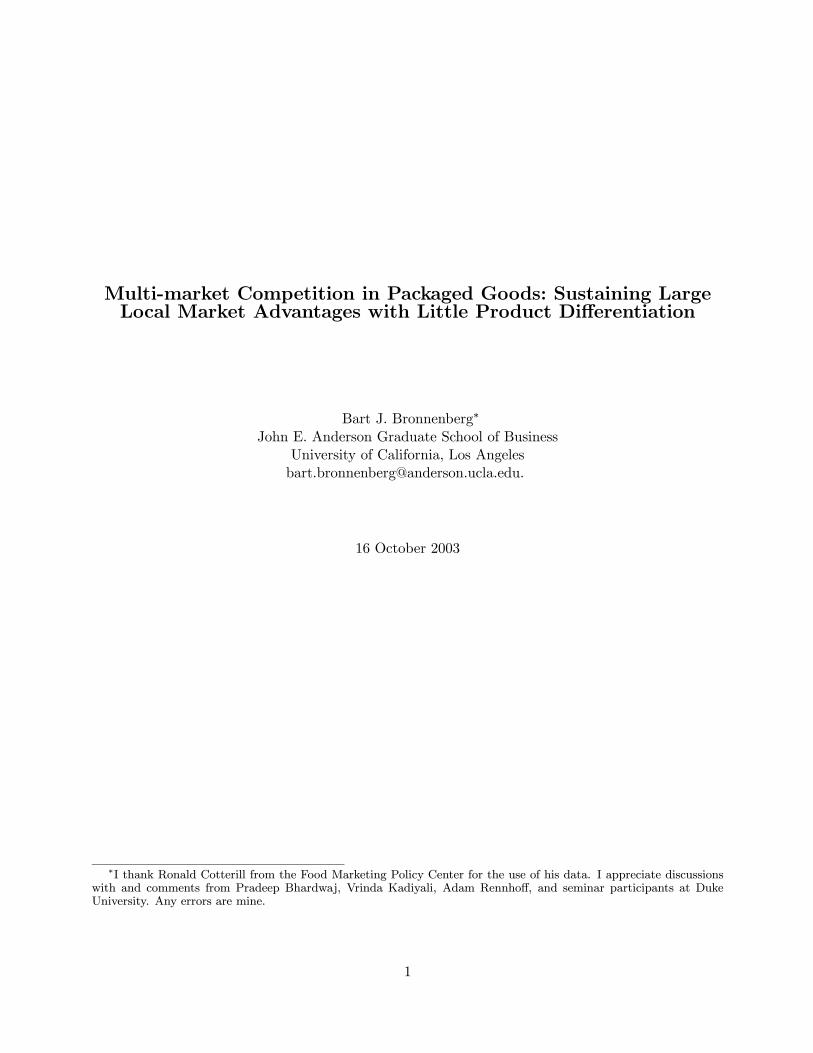
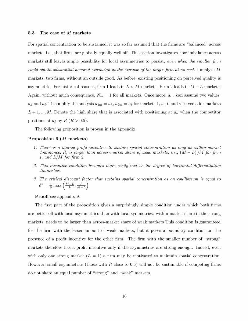
brands. Consider Figure 1, which shows market shares for the two largest manufacturers of brands

of Mexican salsa, Campbell and Frito-Lay. These manufacturers market the Pace and Tostitos

brands, respectively. Both brands originate in Texas and offer very similar products. Within and

across markets, the two firms have very different shares and seem to divide the domestic U.S. market

in two territories, one for each firm.1 Tostitos dominates along the East Coast, whereas Pace leads

west of the Mississippi. While market-shares are clearly not constant across markets, they are in fact

constant across time.2 Given any one market, and given the similarity of the two brands, the question

in this paper is: How is it possible that in direct competition, these firms sustain such diverse yet

persistent market divisions? Put differently, why can large local market advantages persist in the

face of little product differentiation?

I present two explanations for this puzzle. First, reciprocal local market advantages, e.g., where

all competitors have some strong —and accept some weak— markets, can be sustained as the out-

come of multi-market competition. Second, when it is costly to position as the market leader in

communication— or distribution channels, it is still possible for two physically identical products to

end up in an asymmetric equilibrium, even in a single market (i.e., without reciprocity).

With both arguments, the key contingency in this paper is that with less product differentiation,

asymmetries in competitive equilibria occur more often and — if they rely on orientation toward

future profits — are more easily sustained.

Traditionally, geographic concentration of outputs and prices has been linked to geographic cost

1The pattern in Figure 1 is not exceptional. Equally concentrated patterns are observed for categories such asground coffee, margarines, and mayonnaise.

2This fact is illustrated by the fact that Figure 1 represents the annual averages of market shares for 1996, suggestingthat the differences in share are not simply due to temporary local marketing programs.

3

Campbell

min:0.09 max:0.75

Frito Lay

min:0.09 max:0.47

Figure 1: Market shares of two leading manufacturers of mexican salsa

differences (see e.g., Greenhut 1981). For instance, prices can be affected by the location of firms

through transportation cost (Anderson and de Palma 1992; Fujita, Krugman, and Venables 1999).

Thus, locating oneself closer to consumers creates a cost advantage which may impact observed

outputs. In this research tradition, it is the transportation cost of firms that drives the spatial

distribution of prices and outputs.

However, the location of the manufacturers whose outputs are represented in Figure 1 was initially

similar and therefore transportation cost of firms does not to seem to explain the observed data well.

Rather than focusing on the transportation cost of firms, I focus on (1) the transportation cost of

consumers and (2) that firms compete in multiple geographic markets.

Geographic markets are defined in this paper as areas without consumers overlap and without

consumer arbitrage. In other words, I use as a defining characteristic of a geographic market that

consumers do not travel from one market to the next to benefit from price differences across mar-

kets. This definition is particularly applicable in the domestic US with its discrete population centers

(metropolitan areas) separated by sparsely populated space. In the context of packaged goods, con-

sumer transportation cost across such markets is often high compared to the potential gains from

traveling. Although almost entirely omitted from theoretical analysis, the “no consumer arbitrage”

property of local markets is important to understanding multi-market conduct of firms. At a mini-

mum, the opposite assumption, i.e., that firms would not seek to benefit from the de facto immobility

of consumers across markets, seems lacking as a theoretical point of departure.

4

Allowing firms to set different prices in different markets, I show that firms have an incentive

to maintain advantages that may have grown historically in some markets and accept historical

disadvantages in other markets. This incentive increases as the differentiation between products

diminishes and may lead to implicit coordination by firms across markets. Therefore, even without

transportation cost arguments and even with the same types of consumers across markets, large

market advantages can be sustained, especially in the face of little product differentiation.

This paper aims to contribute to a growing literature in economics and marketing about the

role of geography and space. In this context, the “New Economic Geography” (Fujita, Venables,

and Krugman 1999) focuses on providing answers to two fundamental questions about economic

activity. These are (1) when does spatial symmetry of economic activity break, and (2) why do

spatial asymmetries in economic activity persist. Because of the empirical observation of existing

spatial concentration in packaged goods categories, I focus in this paper on the second question.

The paper is organized as follows. The next section reviews research that suggest consumers

take non-product attributes such as advertising and distribution as perceptual cues for product

quality. Section 3 discusses the demand model with local quality perceptions. Section 4 sets up

firm competition and establishes the basic relation between profits, perceived quality and prices in a

single market framework. Section 5 analyses when asymmetries can be sustained in a multi-market

economy even when it is costless to locally reposition from low to high perceived quality. Section 6

shows how the asymmetries can be sustained when there are significant costs to locally positioning

as a high quality firm. It also focuses on the role of retailers in sustaining spatial concentration

of outputs. Section 7 discusses and interprets the main results in the context of packaged goods.

Section 8 concludes.

2 Local determinants of consumer quality perceptions, mind— andshelf-space.

Consumers form brand perceptions from environmental cues other than the product itself. As

Keller (1993) puts it “although the judicious choice of brand identities can contribute significantly to

customer-based brand equity, the primary input comes from [...] the various product, price, advertis-

ing, promotion, and distribution decisions.”

Obviously, an important impetus to quality perceptions remains the physical product itself.

5

However, as the quote above seems to imply, perceptual advantages for packaged goods also originate

in differences in brand awareness and brand support in the distribution channel. Corstjens and

Corstjens (1995) note that brand awareness and distribution support are frequently zero-sum “assets”

to firms because of limits on consumer information processing and on retailer shelf-space. The

premise of this paper is that brand awareness and distribution support such as shelf-space are used

by consumers as quality cues.

For instance, Kirmani and Wright (1989) find a positive relation between advertising and ex-

pectations about product quality. It is therefore not surprising that brand awareness is often a

determinant of choice, especially for low involvement decisions (Bettman and Park 1980; Hoyer and

Brown 1990; Park and Lessig 1981).

Simonson (1993) concludes that consumers construct preferences at the point of purchase. For

packaged goods this means that preferences for different brands are often formed at the supermarket

shelf. Shelf space allocations then affect choices in at least two ways. First, consumers may take

large shelf space allocations of packaged goods as cues that those brands are popular in a given local

market. Thus, if consumers do not acquire brand information themselves (Dickson and Sawyer 1990,

Hoyer 1984), they may rely on (what they believe are) the preferences of others. Second, the spatial

arrangement of products including shelf-space allocations raise brand awareness at point of purchase

(Fazio, Powell, and Williams, 1989).

In sum, while consumers from different markets may face the same physical product, perceptions

about the quality of these products are co-determined by local advertising and distribution strategies

of firms. It is exactly the point of this paper that even if such influences on quality perceptions are

small they can be of substantial consequence in multi-market competition.

I consider two types of perceived quality. In section 4 and 5, I use a concept of perceived quality

that is an endowment from the past. Its cost is sunk. An example is order-of-entry effects on top-

of-mind awareness for brands or on favorable treatment by retailers (Bowman and Gatignon 1990;

Robinson and Fornell 1985). In section 6, perceived quality is costly.

3 A duopoly model of demand

Utility I use an address model of consumer demand. In this model, consumers h are characterized

by a position zh in a K-dimensional attribute space in RK . Whereas the consumer’s ideal point zh

6

is unobserved, its distribution across h is known. Products i = 1, 2 are defined by a known address

zi ∈ RK in the attribute space. Consumers h have a quadratic disutility for distance between ideal

points zh and the location of products zi (d’Aspremont, Gabszewicz, and Thisse 1979). Utility for

brand i by household h = 1, ..., Nm in market m is given by

Vi(h,m) = Yh + aim − pim − µ2

KXk=1

(zkh − zki )2, (1)

where Yh is income of household h, and aim is the perceived quality of a firm in given market. The

local quality attribute aim is common to all households in market m; pim is the price of the product

in market m. The scalar µ measures the consumer’s disutility of products being far away from his

ideal point. The utility model (1) thus acknowledges the presence of household, market, and brand

specific components.

Quality perceptions As discussed previously, quality perceptions can either reflect historical

advantages, such as order of entry effects, selective consumer learning, etc., or can be influenced by

shelf-space allocations by retailers in local markets or local advertising of the brand. Alternatively,

the quality perceptions aim can capture versions of the same product. For instance, services in the

airline industry are spatially versioned, with individual firms offering more travel flexibility in some

regions than in others (see e.g., Karnani and Wernerfelt 1985). However, we focus on the first two

interpretations, i.e., market reach or historical advantages.

Product positions in the physical attribute space I assume that there is one physical attribute

zki (K = 1), in addition to the quality perceptions aim. This attribute is common to all consumers

and markets. To rule out a consumer-focused explanation of asymmetries, I initially assume that

the location of products and consumers is symmetric around zero. Owing to the presence of the

multiplier µ, it can be assumed without loss in generality that the position of product 1 is given by

−12 and of product 2 by +12 . The difference in positions of the two products introduces horizontal

differentiation in the model.

Location of consumers in the physical attribute space The consumer ideal points zh ∈ Rrepresent the idiosyncratic component of utility. I assume the logistic density for the location of

consumers

g(z) =exp−z

(1 + exp−z)2 , z ∈ R1. (2)

Expected demand Consumers choose that alternative that maximizes their utility. Expected

7

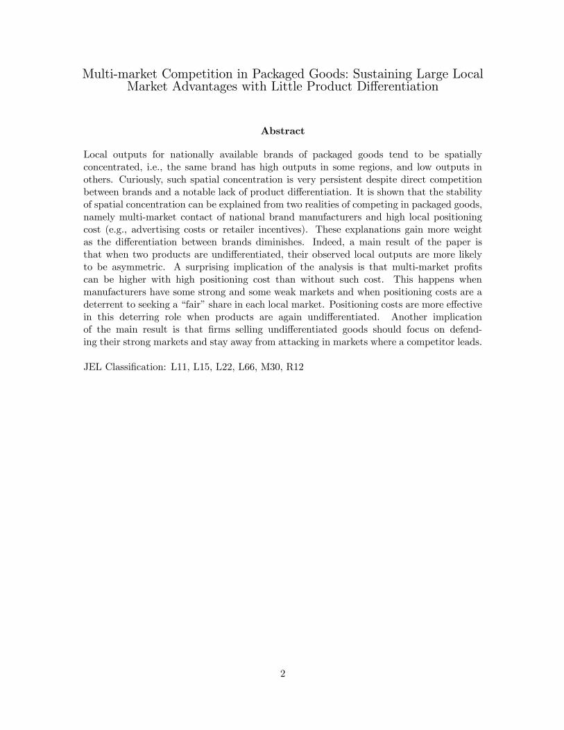
demand of product i for Nm consumers in market m is thus obtained by integrating of the utility

equation (1) over the support of product i using the consumer density of equation (2). Given the

formulation of the utility function the components Yh and z2h, do not affect choice (they are common

to both alternatives). Given the symmetric positions, the utility component z2i (i = 1, 2) also drops

out of the utility comparisons. What remains is the interaction zhzi of the location of consumers

and products. Thus the location of the consumers enters the utility comparison as a linear term,

and hence demand is given by a logit model.

sim = Nm Pr (Vi(h,m) ≥ Vj(h,m)) (3)

= Nm Pr

µzh ≤ (aim − pim)− (ajm − pjm)

µ

¶= Nm

exp [(aim − pim)/µ]P∀j exp [(ajm − pjm)/µ]

, i, j = 1, 2

In this formulation, the effective degree of horizontal differentiation manifests itself as the disutility

for quadratic distance between product i and the consumer’s ideal point scale parameter of the logit,

µ. For convenience and because its role turns out to be largely passive, I arbitrarily scale Nm = 1.

The logit demand formulation has broad appeal in both theoretical (e.g., Anderson, de Palma,

and Thisse 1992), as well as empirical work (e.g., Berry, Levinsohn, and Pakes 1995). It is noted

that with a uniform distribution for g(z), a version of the Hotelling model obtains that is a duopoly

version of the Mussa-Rosen model. This does not change basic results in this paper.

Because I initially wish to separate multi-market contact effects from demand expansion, the

standard model used here does not account for an outside good. This may be justified by realizing

that for mature categories such as coffee, Mexican salsas, and alike, demand expansion is small

(Nijs et al 2002). Nonetheless, it is desirable to explore the robustness of the main results to the

introduction of an outside good. Hence, after establishing several results with the standard model,

these results will be shown to generalize to the case of demand with an outside good.

4 Perceived quality, prices and profits

4.1 A basic relation

Of initial interest is how perceived quality aim, affects prices pim, and profits πim. Firms compete

by first simultaneously setting aim. Conditional on product positioning, firms next simultaneously

8

set prices.3 Marginal cost cim and fixed cost Kim are initially quality-independent and fixed. Thus,

for now, firms can increase perceived quality at no additional cost. This assumption gives a strong

result. If firms do not wish to increase perceived quality to the highest attainable level in each market

even when it is costless to do so, they will not do so when attacking is expensive.4

In a two-product case, demands are give by

s1m =exp [(a1m − p1m)/µ]

exp [(a1m − p1m)/µ] + exp [(a2m − p2m)/µ] , (4)

with s2m = 1 − s1m in the absence of an outside good. The profit function for firm i is πim =

(pim − cim) · sim −Kim.Given the sequence of decisions, prices are solved first. Caplin and Nalebuff (1991) have shown

that a unique Bertrand-Nash equilibrium in prices exists for the demand system in equation (4).

Rearranging the f.o.c. for firm i

dπimdpim

= (pim − cim) · s0im + sim = 0, (5)

an implicit equation for the prices of interest is obtained

p∗im − cim =µ

1− sim , i = 1, 2. (6)

These price equations are implicit because the right-hand side of the expression for the markup

contains all prices, and positioning information (through sim). Using the last equation to solve for

sim and substituting in the profit function gives that at optimal prices

π∗im = p∗im − cim − µ−Kim. (7)

Define the local positioning difference as am ≡ a1m − a2m. Two useful dependencies of local prices(and profits, given the last equation) on the positioning differential are given in the first proposition.

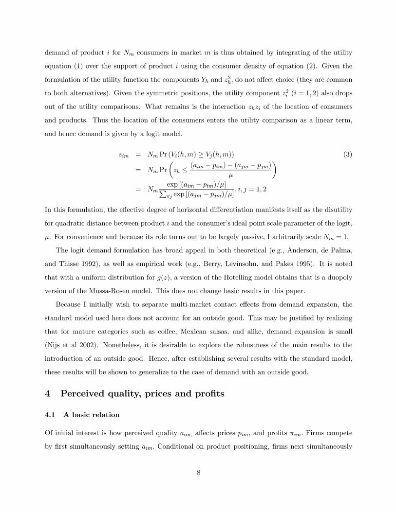
Proposition 1 (Optimal Prices)

1. The price of firm 1’s product is increasing in am, and the price of firm 2’s product is decreasingin am.

2. The price increase (decrease) is never larger than the increase in the positioning differential,i.e.,

0 <dp∗1mdam

< 1, and − 1 < dp∗2mdam

< 0

3Currently these prices are to be interpreted as market prices. Later when the case of retailers is considered, themanufacturers will set whole sale prices.

4I later consider cases where costs depend on aim.

9

Proof: see appendix A

This result states that prices for firm 1 increase as its positioning advantage over firm 2 widens.

However, if one firm improves its positioning, its equilibrium price does not rise in equal measure.

Consumers get at least part of the utility stemming from positioning improvement. For a related

result, see Anderson, de Palma and Thisse (1992), and Anderson and de Palma (2001).

Proposition 2 (Convexity) The optimal prices of both products, p∗1m and p∗2m are convex in theirpositioning difference, am.


This result states that with a widening positioning gap between the two products, the marginal

effect of am = a1m − a2m, m = 1, ...,M, on prices increases. Given equation (7) this result also

applies to profits.

What does this result imply for multi-market profits? First, firms can set aim in each market.

The convexity result then implies that both firms, competing on M markets, would prefer to have

a distribution of uneven market-specific positions am over an even set of product positions of a =

1M

Pam in each market.

In practical terms, the result therefore suggests that each firm is better off having some strong

markets paired with some weak markets rather than having many “average” markets. Both firms

therefore have an incentive to sustain uneven market-division as long as each firm has a sufficient

number of “strong” markets: a condition to be explored more fully in the coming sections. I now

present a benchmark result in a single market.

4.2 The case of a single market

Suppose firms can choose among two levels of perceived quality ah and a`, with ah > a`. Firms first

set perceived quality aim simultaneously and subsequently choose prices. The following proposition

conveys that, in a single market, both firms will end up positioning at ah.

Proposition 3 (Single Market) In the single market equilibrium both firms position at ah andcharge a price of c+ 2µ. Profits are equal to µ−K.


That is to say, given proposition 1 both firms choose to set perceived quality high. This will give

both players equal shares in the market and give the optimal prices in the market. As expected,

10

profits and prices rise in the degree of horizontal differentiation.5 In other words, if horizontal

differentiation is effectively absent, price competition will drive profits to zero.

I now consider how the above result can be avoided as a function of a key reality of firm com-

petition in packaged goods, namely that firms meet in multiple markets that are characterized by

absence of consumer arbitrage.

5 Sustaining historical asymmetries through multi-market contact

5.1 Spatial concentration and horizontal product differentiation

The base-scenario analyzed in this section contains two firms, two markets, and two levels of perceived

quality: high (ah) and low (a`). For the moment, firms can increase perceived quality from low to

high at no cost. Firms each maximize multi-market profits by choosing positioning aim first, and

setting prices pim next. In addition, in a multi-market context, it is unnecessarily restrictive to limit

the analysis to one-period games. Therefore, firms are allowed to interact repeatedly in an infinite

horizon game (Bernheim and Whinston 1990).6

Consistent with empirical observation, e.g., Figure 1, it is assumed that there is an existing degree

of spatial concentration in outputs. In the modeling framework, this translates in each firm being

endowed with one market in which it is the sole provider of a high perceived quality product and

one market in which it is the sole provider of a lower perceived quality product. This pre-existing

condition is exogenous to the analysis and its origins are therefore left general. The analysis therefore

applies to the persistence of any type of local advantages, even those whose origins are fleeting.

Arbitrarily let firm 1 be positioned at ah in market 1 while firm 2 is positioned at a`. In market 2

the opposite happens. Denote the ratio of output of product 1 to that of product 2 at optimal prices in

market 1 by Φ ≡ s∗11/s∗21. Further, denote the equilibrium profits of firm i by π∗i ≡Pm π∗im = π∗i1+π

∗i2.

Given equal cost, the prices of products mirror each other across markets, i.e. p∗11 = p∗22, and

p∗12 = p∗21. From the definition of the ratio of outputs, it is therefore obvious that in market 2,

s∗12/s∗22 = Φ−1. By proposition 1, Φ > 1, i.e., in market 1, firm 1 is the product with the higher

5Soberman (2002) shows however that in a single market, if consumers differ with respect to their awareness ofproducts, the monotonicity of profits in differentiation may not hold.

6Comparisons to the single period single market game in the previous section are thus not immediate. However,unless consumers accept the idea of each firm taking periodic turns at being the “high-quality” player, a single marketrepeated game will result in the same equilibrium as the single period game.

11

perceived quality, prices, and demand. Equations (6) and (7) give that

π∗im =sim

1− sim · µ−K (8)

Therefore, with asymmetric positioning, multi-market profits are

π∗i =Xm

π∗im =¡Φ+Φ−1

¢µ− 2K, i = 1, 2. (9)

If quality positioning is free, firm 1 is tempted in the short run to reposition from a` to ah in market

2. Because both products are then positioned at ah in market 2, the ratio of their outputs is 1. Thus,

the one-time payoff of deviation for firm 1 is πd1 = (Φ+ 1)µ − 2K. Given this deviation, it is easyto show that firm 2 now optimally repositions in market 1 from a` to ah. The payoff for both firms

is now equal to π0i = 2µ − 2K. Subsequently, there is no profitable deviation for either firm. Thefollowing proposition now holds:

Proposition 4 (base result)

1. There is always a mutual profit incentive to sustain spatial concentration.

2. The minimum discount factor that sustains spatial concentration is equal to the ratio of eachfirm’s smaller and larger output, i.e., δ∗ = Φ−1

3. The motivation to sustain spatial concentration decreases monotonically with the degree ofproduct differentiation.


The first part of the proposition states that π∗i > π0i , i.e., that there is always a profit incentive

to sustain spatial concentration. This result is implied by proposition 2. Indeed, with asymmetric

positioning the positioning difference in market 1 is a1 = ah−a`, whereas in market 2 it is −a1. Thepositioning difference when both competitors position at ah is equal to 0 in both markets. It follows

from the proposition that π(a1) + π(−a1) > 2π (0).The second part of the proposition implies that existing spatial concentration is sustainable —even

when breaking it is free— as long as firms value future profits sufficiently. Specifically, firm 1 does

not reposition if a periodic profit of π∗i , is valued higher than a one time profit of πdi followed by a

periodic profit of π0i . This valuation is met for all discount rates δ that satisfy

π∗i (1 + δ + δ2 + · · ·) > πdi + π0i (δ + δ2 + δ3 · · ·). (10)

Hence, when

δ > δ∗ ≡ πdi − π∗iπdi − π0i

=1

Φ(11)

12

firm 1 does not reposition. By symmetry, the same holds for firm 2. Given that Φ > 1 by construction,

0 < δ∗ < 1. As a matter of interpretation, the more asymmetric existing outputs are, the less forward

looking managers need to be to sustain them.

The third part of the proposition is based on the result that ∂δ∗/∂µ > 0. This result implies that

as markets are less and less differentiated, even myopic managers will sustain spatial concentration.

This is for two reasons. First, the profit gains from improving one’s position in the weak market is

not large when there is no product differentiation. That is, the short-term incentive to deviate is

less. Second, the post-deviation drop in profits from competing head-to-head looms larger in absence

product differentiation. Indeed, as the horizontal differentiation of the products diminishes, the value

of δ∗ tends to zero.

5.2 Duopoly with outside good

The previous analysis generated an unconditional result because it isolated one specific aspect of

multi-market competition, namely, that spatial concentration creates local market power for both

firms. However, it is likely that breaking the spatial concentration by positioning both products

at ah raises category-demand. To investigate which of these effects (market power vs. demand

expansion) dominates, I investigate positioning and pricing decisions in the presence of an outside

good. Demand is now given by

sim = Nm · exp [(aim − pim)/µ]exp [(a1m − p1m)/µ] + exp [(a2m − p2m)/µ] + exp [V0/µ] , i = 1, 2, m = 1, 2,

where V0 is the value of the outside good. As before, set Nm = 1 in both markets.7

Equation (6) still describes optimal prices given positioning. To facilitate discussion of the results

in the presence of an outside good, some additional notation is helpful. Let T stand for the combined

share of the inside goods (at optimal prices) when both are positioned at ah. S is the combined share

of the inside goods (again at optimal prices) when one is positioned at ah and the other at a`.

Finally, among the inside goods, R is the share of the product positioned at ah if the other product

is positioned at a`, i.e., R = s1/(s1 + s2), if product 1 is positioned at ah and product 2 at a`.

Applying these definitions, s1 = SR if product 1 is positioned at ah and product 2 at a`, whereas

s1 = 0.5T if both products are positioned at ah. The following result holds.

7A more general result can be obtained using a nested logit model with separate nests for the inside and outsidegoods and different scale parameters for the choice among nests and the choice among the inside goods. The results forthis model are analytically very cumbersome without adding much insight. These results are available upon request.

13

Proposition 5 (Outside good)

1. There is a mutual profit incentive to sustain spatial concentration as long as the demand ex-pansion effects is not too large. More formally,

T − S < S2 (1− 2R)2(2− S) .

2. If the above inequality holds, the minimum discount factor that sustains spatial concentrationequals,

δ∗ =1

Φ

TΦ− S (2− T )S (2− T )Φ− T

where Φ = R/ (1−R)Proof: see appendix A

The interpretation of the first part of the proposition is as follows. The right hand side of the

inequality is always positive. Hence as long as T − S ≤ 0, the presence of a pay-off incentive to

sustain any existing asymmetries is guaranteed. However, the more interesting case is T − S > 0

(demand expansion from both positioning at ah). The proposition states that as long as demand

expansion from both products positioning at ah is not too large, there is a profit incentive to maintain

a reciprocal form of asymmetric positioning. Because previous research (e.g., Nijs 2002) suggests

that expansion effects (at least those of price) are small in mature categories, this condition seems

met in practice. In addition, T −S is likely to be small for undifferentiated products. If the productsare the same, then increasing the perceived quality of one of them while the other is already of high

quality should not affect their cumulative demand appreciably. This is not the case for differentiated

goods where increases in perceived quality draw demand that is unique to each product.

The second part of the proposition shows δ∗ to be a rather complex function of S, T, and Φ. It

is noted that when the outside good gets smaller (and S and T tend to 1) the same expression as in

proposition 4 will obtain.

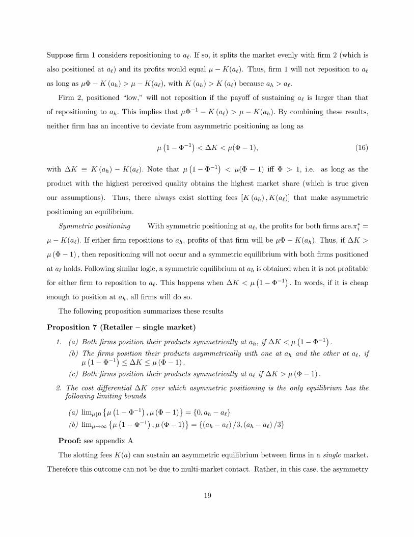
In order to illustrate when spatial concentration is more profitable than symmetric positioning

even in the presence of an outside good, I use an example of profits under spatial concentration vs.

symmetric positioning as a function of µ. Figure 2 shows the multi-market profits at optimal prices

when ah = 1, a` = 0, and V0 = −1 as a function of µ. As is clear from the graph, for small degrees of

horizontal differentiation, the profit incentive to sustain asymmetries is present and given sufficient

valuation of future profits asymmetric positioning is an equilibrium.

Two aspects of the profit curves are noteworthy. Profits decrease in the degree of horizontal

differentiation, µ, for µ small enough. Thus, spatially concentrated industries with “intermediate”

14

0 0.2 0.4 0.6 0.8 1 1.2 1.4 1.6 1.8 20

0.2

0.4

0.6

0.8

1

1.2

1.4

mul

timar

ket p

rofit

µ

spatial concentration

symmetric positioning

B

C

A

Figure 2: Multimarket profits with symmetric and with asymmetric positioning

levels of product differentiation are less profitable than industries without product differentiation (see

also Klemperer 1992 who raises a similar point). Point A in Figure 2 shows that profits from spatial

concentration are 1 when there is no horizontal differentiation, i.e., µ = 0. Not until a relatively high

degree of horizontal differentiation, µ = 1.47, is there a multi-market policy with equal profits (point

B). The intuition of the negative impact of µ on profits is that differentiation on perceived quality is

more effective when there is no actual horizontal differentiation between the products. The demand

effect of positioning aim is amplified (dampened) by absence (presence) of horizontal differentiation.8

Second, in the presence of an outside good, the two profit curves intersect (this is the condition-

ality in the first part of proposition 5). Hence, beyond a certain degree of horizontal differentiation

firms are more profitable when they both position as high quality players.

8While our main results so far are insensitive to the choice of a logit vs. linear demand system, the decrease inprofits with increased differentiation is specific to the logit demand system and does not hold with a linear demandsystem.

15

5.3 The case of M markets

For spatial concentration to be sustained, it was so far assumed that the firms are “balanced” across

markets, i.e., that firms are globally equally well off. This section investigates how imbalance across

markets still leaves ample possibility for local asymmetries to persist, even when the smaller firm

could obtain substantial demand expansion at the expense of the larger firm at no cost. I analyze M

markets, two firms, without an outside good. As before, existing positioning on perceived quality is

asymmetric. For historical reasons, firm 1 leads in L < M markets. Firm 2 leads in M −L markets.Again, without much consequence, Nm = 1 for all markets. Once more, aim can assume two values:

ah and a`. To simplify the analysis a1m = ah, a2m = a` for markets 1, ..., L and vice versa for markets

L + 1, ...,M. Denote the high share that is associated with positioning at ah when the competitor

positions at a` by R (R > 0.5).

The following proposition is proven in the appendix.

Proposition 6 (M markets)

1. There is a mutual profit incentive to sustain spatial concentration as long as within-marketdominance, R, is larger than across-market share of weak markets, i.e., (M − L) /M for firm1, and L/M for firm 2.

2. This incentive condition becomes more easily met as the degree of horizontal differentiationdiminishes.

3. The critical discount factor that sustains spatial concentration as an equilibrium is equal to

δ∗ = 1Φ max

³M−LL , L

M−L´


The first part of the proposition gives a surprisingly simple condition under which both firms

are better off with local asymmetries than with local symmetries: within-market share in the strong

markets, needs to be larger than across-market share of weak markets This condition is guaranteed

for the firm with the lesser amount of weak markets, but it poses a boundary condition on the

presence of a profit incentive for the other firm. The firm with the smaller number of “strong”

markets therefore has a profit incentive only if the asymmetries are strong enough. Indeed, even

with only one strong market (L = 1) a firm may be motivated to maintain spatial concentration.

However, small asymmetries (those with R close to 0.5) will not be sustainable if competing firms

do not share an equal number of “strong” and “weak” markets.

16

The second part of the proposition states that, in the case of M markets, as was the case for a

2 market duopoly, the profit incentive to sustain asymmetries is more generally present when firms

are less horizontally differentiated. Technically, the smaller µ, the larger R.

The third part of the proposition focuses on the critical discount factor that sustains the scenario

of this section as an equilibrium in which one firm has L strong markets and one firm has M − Lstrong markets. Mathematically, the discount factor is equal to the relative within-market share

(1−R) /R in weak markets (at optimal prices) times the relative across-market share of weak markets(M − L) /L. Given that this result only holds if there is a principle reason to sustain asymmetricpositions, this discount rate is guaranteed to be less than 1. The max operator in the third part

of the proposition expresses the condition that the firm with the lesser number of strong markets

is more easily tempted to attack in its weak markets. The result in proposition 4 that dΦ/dµ < 0,

implies that —as before— even relatively impatient managers will resist the short term temptation to

attack and increase their demand in “weak” markets when product differentiation diminishes.

6 The role of positioning cost: the case of retailers

6.1 A simple representation of retailers

To discuss the role of local positioning cost on sustaining multi-market spatial concentration, I use

a contextual example. This example interprets positioning costs as retailer fees paid by competing

firms in order to obtain “premium” shelf space. Admittedly, other interpretations of such costs, e.g.,

advertising costs, are equally judicious in the context of consumer packaged goods. To allow for

some generality in interpretation, positioning costs are modeled using two simple modifications to

the model.

First, slotting fees,9 promotion allowances, and alike are modeled as a (periodic) fixed cost, K,

that does not depend on quantity sold. It is assumed that retailer support for firm i in market m

enhances the quality perceptions of consumers aim. The fixed cost K(a) increases in a and is assumed

to be low enough for two manufacturing firms to enter in any given market. The latter accords with

the empirical fact that all local markets are entered by multiple manufacturers.

The second modification is the introduction of a fixed retailer mark-up. Prices are modeled as

9Slotting fees are meant here to capture “pay-to-stay” fees. Such fees are charged by retailers to manufacturers inreturn for special treatment at the supermarket shelf. See e.g., Federal Trade Commission (2001).

17

pim = wim+ uim, where uim is the markup set by all retailers in market m and wim is the wholesale

price that is set by the firm. I use constant retailer mark-ups uim = u, because these retailer mark-ups

reflect intra-market competitive phenomena (e.g., competition between retailers) that do not likely

give rise to spatial concentration at the national level (for a similar simplification, see Vilcassim,

Kadiyali, and Chintagunta 1999).

Exogenous slotting fees and markups are a useful approximation of the reality that retailers face

many different product categories and therefore use heuristic approaches to setting margins and

slotting fees. Even with passive retailers, the model is informative about how the presence of costly

retailers might sustain spatial concentration.

6.2 Single market competition

Consider a single market (drop the subscript m momentarily), logit demand, no outside good, two

manufacturing firms, and the presence of retailers with slotting fees K(ai), and markup u. Manufac-

turers first set positioning simultaneously, and then simultaneously decide on prices. I again assume

that there are two possible levels of quality perceptions ah and a`. Demand for good i is equal to

si =exp ((ai − pi)/µ)

exp ((a1 − p1)/µ) + exp ((a2 − p2)/µ) (12)

with pi = wi + u. In a single market context, profit for each of the manufacturing firms is equal to

πi = si (wi − c)−K (ai) (13)

From the first-order conditions, wholesale prices are equal to

wi = c+µ

1− si . (14)

Note that these prices are not the same as before. That is to say, the retailer mark-up is represented

in the shelf price, which in turn impacts si. Profits at these wholesale prices are equal to

π∗i =µsi1− si −K (ai) . (15)

Of initial interest is whether an asymmetric equilibrium in which one firms positions at ah and the

other at a` can emerge because of slotting fees K(a).

Asymmetric positioning Consider first the case where product 1 is positioned at ah while

product 2 is positioned at a`. Profit for firm 1 is equal to π∗1 = µΦ−K (ah) , with Φ = s1/ (1− s1) > 1.

18

Suppose firm 1 considers repositioning to a`. If so, it splits the market evenly with firm 2 (which is

also positioned at a`) and its profits would equal µ −K(a`). Thus, firm 1 will not reposition to a`

as long as µΦ−K (ah) > µ−K(a`), with K (ah) > K (a`) because ah > a`.Firm 2, positioned “low,” will not reposition if the payoff of sustaining a` is larger than that

of repositioning to ah. This implies that µΦ−1 −K (a`) > µ −K(ah). By combining these results,

neither firm has an incentive to deviate from asymmetric positioning as long as

µ¡1− Φ−1¢ < ∆K < µ(Φ− 1), (16)

with ∆K ≡ K (ah) − K(a`). Note that µ¡1−Φ−1¢ < µ(Φ − 1) iff Φ > 1, i.e. as long as the

product with the highest perceived quality obtains the highest market share (which is true given

our assumptions). Thus, there always exist slotting fees [K (ah) ,K(a`)] that make asymmetric

positioning an equilibrium.

Symmetric positioning With symmetric positioning at a`, the profits for both firms are.π∗i =

µ−K(a`). If either firm repositions to ah, profits of that firm will be µΦ−K(ah). Thus, if ∆K >

µ (Φ− 1) , then repositioning will not occur and a symmetric equilibrium with both firms positioned

at a` holds. Following similar logic, a symmetric equilibrium at ah is obtained when it is not profitable

for either firm to reposition to a`. This happens when ∆K < µ¡1− Φ−1¢ . In words, if it is cheap

enough to position at ah, all firms will do so.

The following proposition summarizes these results

Proposition 7 (Retailer — single market)

1. (a) Both firms position their products symmetrically at ah, if ∆K < µ¡1− Φ−1¢ .

(b) The firms position their products asymmetrically with one at ah and the other at a`, ifµ¡1− Φ−1¢ ≤ ∆K ≤ µ (Φ− 1) .

(c) Both firms position their products symmetrically at a` if ∆K > µ (Φ− 1) .2. The cost differential ∆K over which asymmetric positioning is the only equilibrium has thefollowing limiting bounds

(a) limµ↓0©µ¡1−Φ−1¢ , µ (Φ− 1)ª = {0, ah − a`}

(b) limµ→∞©µ¡1− Φ−1¢ , µ (Φ− 1)ª = {(ah − a`) /3, (ah − a`) /3}


The slotting fees K(a) can sustain an asymmetric equilibrium between firms in a single market.

Therefore this outcome can not be due to multi-market contact. Rather, in this case, the asymmetry

19

is due to the inherent non-linearity in demand.10 The first two parts of this proposition were discussed

above.

The second part of the proposition merits further discussion and interpretation. When product

differentiation is low, i.e., when µ ↓ 0, the difference in gross profits (before positioning cost) betweenthe two firms in the unit-sized market tends to ah − a`. This statement echoes proposition 1 whichshowed that price (and profit) increases are never larger than the increases in positioning. Therefore,

the upper limit of the difference in slotting fees ∆K that supports an asymmetric equilibrium is equal

to ah − a`.Conversely, when the category becomes more differentiated —as µ increases— positioning has less

influence on profitability. In the limiting case of ever increasing µ, there can only be an asymmetric

equilibrium if (ah − a`) /3 ≤ ∆K ≤ (ah − a`) /3. In other words as the products are more horizontallydifferentiated, no slotting fees (except in the limit K(a) = K0 +

13a) will support an asymmetric

equilibrium.

The width of the intervalnµ³1− (Φ1)−1

´, µ (Φ1 − 1)

ocan be loosely interpreted as the gener-

ality with which an arbitrary cost function K(a), a > 0, obeys µ¡1− Φ−1¢ ≤ ∆K ≤ µ (Φ− 1) . If

the interval is wide, any cost differential will support an asymmetric market outcome as the only

equilibrium outcome. Conversely, if the interval is very narrow, only very small cost-differences will

support an asymmetric market outcome. Hence, again, asymmetric outcomes happen under more

general conditions when goods are undifferentiated. The intuition behind this result is that when

goods are undifferentiated, there is only “room” for one high quality player in the market. If two

products try to both be high quality players, neither of them will make enough profits to make up

for the increased positioning costs.

6.3 Multi-market competition in the presence of retailers

I now consider the case of two markets instead of one. Retailers are again passive players, with a fixed

mark-up and slotting fees, K(a), that depend on the level of support, a, given to the manufacturer’s

products. As before, I use a repeated interaction framework with infinite horizon to explore the

multi-market nature of competition. In each period, firms position their products first (either at ah

10Yarrow (1989) considers the specific case that K (a) = exp(a). Not unlike this paper, he finds that asymmetricequilibria are possible in a single market. For another instance of the latter result see also Moorthy (1988), whomakes the additional argument that the asymmetric equilibrium may be interpreted as a possible advantage of the firstentrant. Both papers focus on asymmetric equilibria in a single market.

20

or a`) and then set prices.

Four possible positioning cases need to be considered. These cases are listed below.

CASE 1 firm 1 firm 2

market 1 a` a`market 2 a` a`


market 1 ah ahmarket 2 a` a`


market 1 ah a`market 2 a` ah


market 1 ah ahmarket 2 ah ah

All other possible combinations merely involve label switching of firms or markets and are there-

fore redundant. Case 1 (positioning low by all firms in all markets) falls under the previous proposi-

tion. If it is too expensive to position at ah in one market, it is also too expensive to position at ah

in multiple markets.

Case 2 can not be a multi-market equilibrium because it can not be the case (given µ and K(a))

that both firms position at ah in one market and at a` in the other. If positioning is cheap enough

for both firms to select ah in market 1, there is a profitable deviation from both playing a` in market

2. Conversely, if advertising is expensive enough for both firms to choose a` in market 1, there is a

profitable deviation from both selecting ah in market 2.

This leaves cases 3 and 4. For logical reasons, I focus first on case 3. Firm 1 leads firm 2 in

market 1 and vice versa in market 2. At optimal prices the ratio of shares of the larger over the

smaller product is denoted by Φ, as before. If case 3 is an equilibrium, both firms have a profit of

π∗i =¡Φ+Φ−1

¢µ− (K (ah) +K (a`)) . (17)

A possible deviation for a given firm is to reposition to a` in the market where it was positioned

at ah. This deviation is attractive when positioning cost is high enough. However, if it is optimal

for one firm to reposition from ah to a` it is optimal for the other firm to do the same in the other

market. The optimality of this repositioning is therefore considered in case 1 and is covered by

proposition 7.

Another deviation is to reposition to ah in the market in which it was positioned at a`. If so, it

ends up with one market in which it positions at ah against a` by its competitor, and one market

where both firms position at ah. This repositioning will give to the firm that repositions the following

profits

πdi = (Φ+ 1)µ− 2K (ah) . (18)

21

This deviation is attractive in the short run to the firm that repositions if the cost of positioning at

ah is small enough. Specifically, comparison of profits gives that if ∆K < µ¡1− Φ−1¢ , then π∗i < πdi

and firm i has a short term incentive to deviate. If this condition is met for one firm in one market,

it logically also meets for the other firm in the other market. Assume that other firm will then also

position at ah (I now obtain case 4). Upon this retaliation from the second firm, the profits for either

firm will forever equal

π0i = 2µ− 2K (ah) , (19)

which is less than π∗i . Using the same arguments as those preceding proposition 4, case 4 will

not occur if firms value future profits enough. These results are formally stated in the following

proposition

Proposition 8 (Retailer — two markets)

1. Wholesale prices are w∗im = µ/ (1− sim) + c, i = 1, 22. When firms meet in multiple markets the following equilibria exist in the presence of a retailer

(a) If ∆K > µ (Φ− 1) then both products position symmetrically at a` in all markets.(b) If µ

¡1− Φ−1¢ ≤ ∆K ≤ µ (Φ− 1) then one product positions at ah and one product

positions at a` in each market.

(c) If ∆K < µ¡1−Φ−1¢ then

i. if the value of future profits exceeds δ∗ times the value of today’s profits both firmswill sustain spatial concentration.

ii. if the firms are myopic, both products position symmetrically at ah in each market.

3. The minimum current value of future profits that sustains an asymmetric multi-market equi-librium is equal to

δ∗ =1

Φ

µ1− ∆K

µ (1− Φ−1)¶<1

Φ


The third part of the proposition implies that the presence of costly retailers generalizes the

existence of a spatially concentrated equilibrium. Namely, comparing propositions 4 and 8, δ∗ is

smaller in the presence of positioning cost than without it. Indeed, retailer fees make attacking

expensive and effectively discourage myopic behavior by firms that would break spatial concentration

without positioning cost.

Figure 3 helps to interpret the proposition further. It outlines the equilibria that exist for an

arbitrary cost function K(a) (subject to the constraint that the profits for both firms needs to be

non-negative) and degree of horizontal differentiation µ. This figure was generated, using a numerical

22

0 0.1 0.2 0.3 0.4 0.5 0.6 0.7 0.8 0.9 10

0.1

0.2

0.3

0.4

0.5

0.6

0.7

0.8

0.9

1

cost

diff

eren

tial

µ

zone I: symmetric positioningat lower quality

zone II: asymmetric positioningin each market

zone III: spatial concentrationwith multi-market contact

zone IV: symmetric posit-ioning at higher quality

Figure 3: Equilibria for product differentiation µ, and cost differential ∆K.

solver, for the scenario in which ah = 1, and a` = 0. Zone I outlines the cases where the cost difference

between positioning high and low is so large that both products position low in all markets. Zone

II represents the cases where a single-market asymmetric equilibrium exists. In this zone, a firm

may lead in both markets, in one, or in none. In none of these cases is there an incentive to deviate

in any single market. Consequently, deviations in multiple markets are also unprofitable. Zone III

identifies when asymmetric equilibria are sustainable in two markets but not in a single market.

Here the cost difference between positioning high or low is so small that in a single market case,

all products would position at ah. However, in a two-market context, firms prefer to sustain spatial

concentration if they value the future enough. Figure 3 was created with δ = 0.75. Thus even if firms

only value next period’s profits at 75% of current profits, the area over which spatial concentration

is sustainable increases very substantially. Finally, zone IV contains all cases where firms position at

ah in all markets. As the firm’s value for future profits increases, the fourth zone will diminish (as

an example if δ = 0.90, zone IV is no longer visible in Figure 3).

23

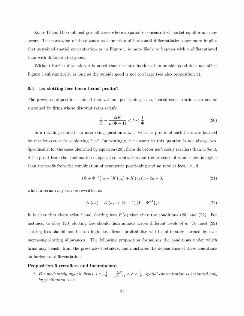
Zones II and III combined give all cases where a spatially concentrated market equilibrium may

occur. The narrowing of these zones as a function of horizontal differentiation once more implies

that sustained spatial concentration as in Figure 1 is more likely to happen with undifferentiated

than with differentiated goods.

Without further discussion it is noted that the introduction of an outside good does not affect

Figure 3 substantively, as long as the outside good is not too large (see also proposition 5).

6.4 Do slotting fees harm firms’ profits?

The previous proposition claimed that without positioning costs, spatial concentration can not be

sustained by firms whose discount rates satisfy

1

Φ− ∆K

µ (Φ− 1) < δ <1

Φ. (20)

In a retailing context, an interesting question now is whether profits of such firms are harmed

by retailer cost such as slotting fees? Interestingly, the answer to this question is not always yes.

Specifically, for the cases identified by equation (20), firms do better with costly retailers than without,

if the profit from the combination of spatial concentration and the presence of retailer fees is higher

than the profit from the combination of symmetric positioning and no retailer fees, i.e., if

¡Φ+Φ−1

¢µ− (K (ah) +K (a`)) > 2µ− 0, (21)

which alternatively can be rewritten as

K (ah) +K (a`) < (Φ− 1)¡1−Φ−1¢µ (22)

It is clear that there exist δ and slotting fees K(a) that obey the conditions (20) and (22). For

instance, to obey (20) slotting fees should discriminate across different levels of a. To meet (22)

slotting fees should not be too high, i.e., firms’ profitability will be ultimately harmed by ever

increasing slotting allowances. The following proposition formalizes the conditions under which

firms may benefit from the presence of retailers, and illustrates the dependence of these conditions

on horizontal differentiation.

Proposition 9 (retailers and incumbents)

1. For moderately myopic firms, i.e., 1Φ − ∆Kµ(Φ−1) < δ < 1

Φ , spatial concentration is sustained only

by positioning costs.

24

2. For such firms, equilibrium profits in the presence of positive positioning cost can be higherthan equilibrium profits without positioning cost. This happens especially when products areundifferentiated, but not when products are horizontally differentiated.


The first part of proposition 9 was addressed above. The last part states that as the horizontal

differentiation between products increases, the firms are better off with retailers only when these

retailers are free. Yet when products are very close substitutes, it is more profitable to have costly

retailers —who sustain spatial concentration— as long as they are not too expensive, i.e., as long as

K (ah)+K (a`) < (ah − a`) (see the Appendix). An interesting link emerges to work by McGuire andStaelin (1983) who found that as products become closer substitutes, firms prefer to shield themselves

from competition by selling through a retailer. In contrast to their single-market framework, the

result here relies on the fact that firms meet in multiple markets.

6.5 An alternative interpretation for advertising

The previous section analyzed the role of positioning cost in the context of shelf space allocations

or other retailer-support. Keller (1993) and Kirmani and Wright (1989) have argued that inferences

about product quality are alternatively affected by advertising investments. Therefore, a short

discussion of the previous results in the context of advertising is appropriate.

In an advertising interpretation, positioning at ah (a`) translates into advertising at a high (low)

level. The cost difference ∆K is the marginal cost of advertising. The previous section suggests

there are three advertising cases to consider.

First, if advertising costs are sufficiently high, nobody will advertise at ah. This is equivalent to

the case in proposition 7 where ∆K is large. Second, for intermediate values of ∆K an asymmetric

advertising equilibrium exists. In such an equilibrium, there is only “room” for one player to advertise

at a high level. The other player will realize that it is impossible to mimic the success of the first

player given that this player occupies the ah position. It is therefore natural to think in this context

of a defensible first mover advantage (see also Moorthy 1988). Finally, for really low values of ∆K

both firms will advertise if the decision makers are strongly myopic.

Advertising expenditures can increase firm profits even if it does not increase demand, especially

for undifferentiated goods. In proposition 9 it was shown that profits with costly positioning can

be higher than profits without costly positioning, even when advertising fails to generate primary

25

demand. In an advertising interpretation, the profitability of advertising comes from the monopoly

power it creates especially in packaged goods industries where goal functions of product managers

are moderately short term oriented (compare equation 20) and where products are undifferentiated.

7 Discussion

The main result of this paper is that spatial concentration may persist especially for products of

undifferentiated consumer goods. This idea was motivated by illustrating the surprising degree of

spatial concentration of weakly differentiated categories such as Mexican salsas. It was noted that

the same degree of spatial concentration holds for products such as ground coffee and mayonnaise.

However, a second result was that opportunities and/or incentives to sustain spatial concentration

are less strong when products are more clearly differentiated.

If the argument about differentiation is empirically important, local differences should not per-

sist to the same extent in categories with differentiated goods. An example of such a category is

breakfast cereals. That is, consumers will in general have little difficulty distinguishing between say

Kellogg’s Corn Flakes and General Mills Cheerios. More broadly, the product portfolios of the top

manufactures contain few if any products that are physically indistinguishable. Indeed, as Nevo

(2001) observes, the top manufacturers of breakfast cereals do not imitate each other’s products.

Therefore, it is not unreasonable to claim that breakfast cereals are more horizontally differentiated

than brands of Mexican salsas.

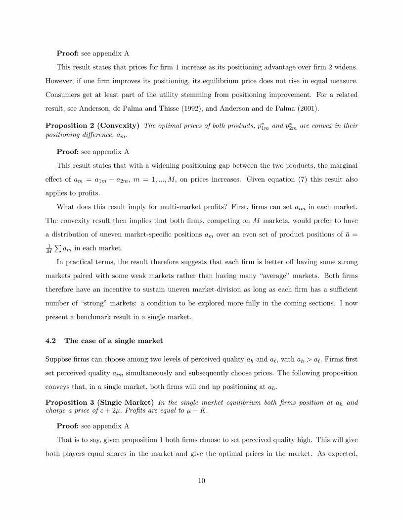
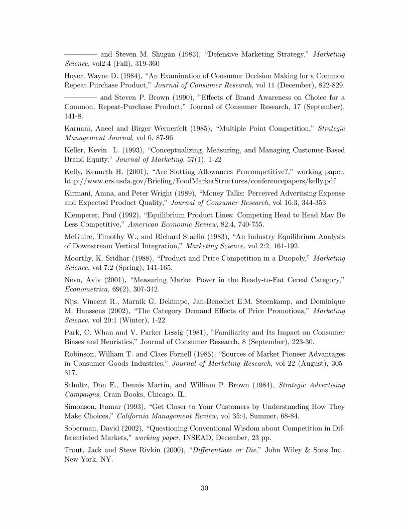
Figure 4 shows the 1992 local shares of Kellogg and General Mills in the breakfast cereal market.

Compared to figure 1, the striking contrast between the salsa data and the cereal data is the absence

of spatial concentration. That is, whereas there are differences in market shares for each product

across markets they are only modest compared to the example of salsas.

This empirical example suggests that (lack of) product differentiation may impact the observed

degree of spatial concentration of an industry. It is not claimed that differentiation is the only

important factor. Specifically, cost efficiencies of spatial concentration or the presence of actors

whose decisions have spatial footprints (such as retailers or distributors) could well contribute to

spatial concentration. However, if the striking difference between figure 4 and 1 is any indication,

the degree of product differentiation does seem to play a role in the occurrence of spatial concentration

of firm outputs.

26

Kellogg

min:0.29 max:0.45

Kellogg

min:0.29 max:0.45

General Mills

min:0.25 max:0.36

General Mills

min:0.25 max:0.36

Figure 4: Local market share of two leading manufacturers in cereals

8 Conclusion

There are many reasons why competing firms of undifferentiated goods face different initial conditions

in a given markets, e.g., order-of-entry effects, pre-emption of mind-space (e.g., selective learning by

consumers) and shelf-space (e.g., selective availability of facings), etc. These phenomena can lead to

initial differences in market shares and profitability. This paper has argued that even after the original

reasons for the asymmetries that arise from such initial conditions vanish, spatial concentration of

prices and outputs can be sustained despite immediate competition between goods. Two different

explanations for this fact were presented.

The first explanation is that multi-market contact provides a mechanism to sustain an implicit

geographical segmentation. As long as each firm has a large enough number of strong markets, or as

long as local domination is strong enough even in a small number of markets, there are no incentives

to compete for “fair share” in each local market once competitive response is taken into account.

The second explanation focuses on the possibility that firms can create a local form of vertical

differentiation through costly positioning of their products through costly agreements with retailers

or costly advertising. It was found that for a variety of positioning cost, there is “room for only one

high quality player in each market.” Thus spatial concentration in multiple markets can be sustained

if local positioning is costly. It is also shown that costly intermediaries such as retailers, may help

to sustain asymmetries by making it expensive for lagging firms to compete for “fair” market share.

27

The contingency that spans both explanations is that sustenance of spatial concentration should

be expected especially when goods are physically similar, i.e., when demand side arguments for spatial

concentration are a priori weak. Surprisingly, if goods are the same, initial market conditions may

cast very long shadows, whereas if products are differentiated, these initial market conditions will

not be sustainable. Indeed, in the latter case, all competitors tend to compete for a “fair share” in

all local markets. Thus in undifferentiated categories, “initial conditions,” i.e., launch strategies, are

very important and may initiate a market division that will resist change.

Provided that spatial concentration leaves both firms with at least some strong markets, this

paper further suggested that profitability of packaged-goods categories does not need to rely exclu-

sively on horizontal product differentiation. Local asymmetries in product positioning on perceived

quality may suffice as a source of differentiation.

Finally, situations wherein category demand is high but market share is low, are oft seen as a

business opportunity (see e.g., Kotler 2003; Schultz, Martin and Brown, 1984). The results in this

paper are cautionary with respect to attacking in such markets. Specifically, in cases of spatial con-

centration a firm has to consider what will happen in one’s own high-share markets as a consequence.

The results in this paper suggest that spatial concentration may dissolve and all firms will be worse

off ever after. This is especially true in mature categories with a low degree of product differentiation,

i.e., for many packaged goods categories.

There are several limitations to this paper. First, I have analyzed duopolies in markets of equal

size. Whereas the consideration of oligopolies or markets of varying size will have some impact

on the results, such impact is small and perhaps of limited theoretical interest. Second, I have

focused mainly on sustenance of existing asymmetries. In future research, it is desirable to address

the emergence of concentrations in market shares. Indeed, given the opportunity of sustenance

of asymmetries especially when there is little product differentiation, the question of what causes

these asymmetries takes on some urgency. Third, empirically —and Figure 1 nicely illustrates this—

the patterns of share concentration are highly spatial. Given the regularity of the patterns, and

the degree of spatial variability of market shares, it seems important to study the origins of this

phenomenon.

28

9 References

Anderson, Simon P., Andre de Palma (1988), “Spatial Price Discrimination with Het-

erogenous Products,” the Review of Economic Studies, vol 55, 573-592.

––––—, ––––— (2001), “Product Diversity in Asymmetric Oligopoly: Is the Qual-

ity of Consumer Goods too Low?” the Journal of International Economics, vol 49,

113-135.

––––—, ––––—, and Jacques-Francois Thisse (1992), “Discrete Choice Theory of

Product Differentiation,” MIT press, Cambridge MA.

Berry, Steven, James Levinsohn and Ariel Pakes (1995), “Automobile Prices in Market

Equilibrium,” Econometrica, vol 63:4 (July), 841-890.

Bernheim, B. Douglas and Michael D. Whinston (1990), “Multi-market Contact and

Collusive Behavior,” Rand Journal of Economics, vol 21:1 (Spring), 1-26.

Bettman, James R. and C. Whan Park (1980), ”Effects of Prior Knowledge and Expe-

rience and Phase of the Choice Process on Consumer Decision Processes: A Protocol

Analysis,” Journal of Consumer Research, 7 (December), 234-48.

Bowman, Douglas, and Hubert Gatignon (1996), “Order of Entry as a Moderator of the

Effect of the Marketing Mix on Market Share,” Marketing Science, vol 15:3, 222-242

Caplin, Andrew and Barry Nalebuff (1991), “Aggregation and Imperfect Competition:

On the Existence of Equilibrium,” Econometrica, vol 59, 26-61.

Carpenter, Gregory S, Rashi Glazer, and Kent Nakamoto (1994), “Meaningful Brands

from Meaningless Differentiation: The Dependence on Irrelevant attributes,” Journal of

Marketing Research, vol 31:3 (Augustus), 339-350.

Corstjens, Judith, and Marcel Corstjens (1995), Store Wars, John Wiley and Sons, New

York, NY.

Dickson, Peter and Alan G. Sawyer (1990), “The Price Knowledge and Search of Super-

market Shoppers,” Journal of Marketing, vol 54 (July), 42-53.

d’Aspremont C., J.J. Gabszewicz, and J.-F. Thisse (1979), “On Hotellings ‘Stability in

Competition,”’ Econometrica, 47:1145-1150

Fazio, Russell H., Martha C. Powell, and Carol J. Williams (1989), ”The Role of Attitude

Accessibility in the Attitude and Behavior Process,” Journal of Consumer Research, 16

(December), 280-8.

Federal Trade Commission (2001), “Report on the Federal Trade Commission Workshop

on Slotting Allowances and Other Marketing Practices in the Grocery Industry,” Febru-

ary, 72 p

Fujita, Masahisa, Paul Krugman, and Anthony J. Venables (1999), “The Spatial Econ-

omy: Cities, Regions and International Trade,” MIT Press, Cambridge, MA.

Greenhut, M.L (1981), “Spatial Pricing in the United States, West Germany, and Japan,”

Economica, vol 48, 79-86

Hauser, John R. (1988), “Competitive Price and Positioning Strategies,” Marketing Sci-

ence, vol 7:1 (Winter), 76-91.

29

––––— and Steven M. Shugan (1983), “Defensive Marketing Strategy,” Marketing

Science, vol2:4 (Fall), 319-360

Hoyer, Wayne D. (1984), “An Examination of Consumer Decision Making for a Common

Repeat Purchase Product,” Journal of Consumer Research, vol 11 (December), 822-829.

––––— and Steven P. Brown (1990), ”Effects of Brand Awareness on Choice for a

Common, Repeat-Purchase Product,” Journal of Consumer Research, 17 (September),

141-8.

Karnani, Aneel and Birger Wernerfelt (1985), “Multiple Point Competition,” Strategic

Management Journal, vol 6, 87-96

Keller, Kevin. L. (1993), “Conceptualizing, Measuring, and Managing Customer-Based

Brand Equity,” Journal of Marketing, 57(1), 1-22

Kelly, Kenneth H. (2001), “Are Slotting Allowances Procompetitive?,” working paper,

http://www.ers.usda.gov/Briefing/FoodMarketStructures/conferencepapers/kelly.pdf

Kirmani, Amna, and Peter Wright (1989), “Money Talks: Perceived Advertising Expense

and Expected Product Quality,” Journal of Consumer Research, vol 16:3, 344-353

Klemperer, Paul (1992), “Equilibrium Product Lines: Competing Head to Head May Be

Less Competitive,” American Economic Review, 82:4, 740-755.

McGuire, Timothy W., and Richard Staelin (1983), “An Industry Equilibrium Analysis

of Downstream Vertical Integration,” Marketing Science, vol 2:2, 161-192.

Moorthy, K. Sridhar (1988), “Product and Price Competition in a Duopoly,” Marketing

Science, vol 7:2 (Spring), 141-165.

Nevo, Aviv (2001), “Measuring Market Power in the Ready-to-Eat Cereal Category,”

Econometrica, 69(2), 307-342.

Nijs, Vincent R., Marnik G. Dekimpe, Jan-Benedict E.M. Steenkamp, and Dominique

M. Hanssens (2002), “The Category Demand Effects of Price Promotions,” Marketing

Science, vol 20:1 (Winter), 1-22

Park, C. Whan and V. Parker Lessig (1981), ”Familiarity and Its Impact on Consumer

Biases and Heuristics,” Journal of Consumer Research, 8 (September), 223-30.

Robinson, William T. and Claes Fornell (1985), “Sources of Market Pioneer Advantages

in Consumer Goods Industries,” Journal of Marketing Research, vol 22 (August), 305-

317.

Schultz, Don E., Dennis Martin, and William P. Brown (1984), Strategic Advertising

Campaigns, Crain Books, Chicago, IL.

Simonson, Itamar (1993), “Get Closer to Your Customers by Understanding How They

Make Choices,” California Management Review, vol 35:4, Summer, 68-84.

Soberman, David (2002), “Questioning Conventional Wisdom about Competition in Dif-

ferentiated Markets,” working paper, INSEAD, December, 23 pp.

Trout, Jack and Steve Rivkin (2000), “Differentiate or Die,” John Wiley & Sons Inc.,

New York, NY.

30

Vilcassim, Naufel J., Vrinda Kadiyali and Pradeep K. Chintagunta (1999), “Investigating

Dynamic Multifirm Market Interactions in Price and Advertising,” Management Science,

45:4, page 499-518

Villas-Boas, Miguel (1993), “Predicting Advertising Pulsing Policies in an Oligopoly: A

Model and an Empirical Test,” Marketing Science, 12:1, 88-102.

Yarrow, George (1989), “The Kellogg’s Cornflakes Equilibrium and Related Issues,” Work-

ing paper, Hertford College, Oxford.

Zeithaml, Valarie (1988), ”Consumer Perceptions of Price, Quality, and Value: A Means-

End Model and Synthesis of the Evidence,” Journal of Marketing, 52 (July), 2-22.

31

A Proofs

Proof of proposition 1 For convenience, drop all subscripts m. Recall that

s1 =exp [(a− p1)/µ]

exp [(a− p1)/µ] + exp [(−p2)/µ] , a = a1 − a2 (A.1)

Some useful relations are ds1dp1

= − 1µs1(1− s1), ds1dp2 = 1µs1s2,

ds1da =

1µs1(1− s1). Taking the first order

condition for firm 1 gives,

F (p1, p2, a) ≡ p1 − c1 − µ

1− s1 = 0 (A.2)

The total differential of this function is Fp1dp1+Fp2dp2+Fada = 0.Writing Φ ≡ s1/s2, it is easy toshow that

Fp1 = 1− µ · d (1− s1)−1

dp1= 1− µ (1− s1)−2 ds1

dp1= 1 +Φ (A.3)

It can further be shown that Fp2 and Fa are both equal to −Φ. Substitution in the total differentialfor F gives

(1 + Φ) dp1 − Φdp2 − Φda = 0 (A.4)

Now, totally differentiate the first order condition for firm 2.

G(p1, p2, a) ≡ p2 − c2 − µ

s1= 0 (A.5)

The total differential of this function is Gp1dp1 +Gp2dp2 +Gada = 0. Once more it is easy to show

that

Gp1 = − 1Φ, Gp2 = 1 +

1

Φ, Ga =

1

Φ(A.6)

Substitution in the total differential of G gives

− 1Φdp1 +

µ1 +

1

Φ

¶dp2 +

1

Φda = 0 (A.7)

Finally, combining (A.4) and (A.7), gives that

dp∗1da

=Φ2

1 + Φ+Φ2> 0,

dp∗2da

=−1

1 +Φ+Φ2< 0. (A.8)

This proofs proposition 1. The result states further that changes in a are never priced by the firm

to the market completely. Indeed, it may be noted from the definition of Φ that the sensitivity of p1to changes in a is always between 0 and 1. ¥

Proof of proposition 2 Once again, the subscript m is dropped from the notation. It

needs to be shown that the profits of both firms are convex in a. Thus, the second order derivative

of profits with respect to a needs to be evaluated at the equilibrium prices. It is sufficient that

d³dπ∗idq

´da

=d2π∗ida2

=d2p∗ida2

> 0, i = 1, 2 (A.9)

32

To simplify the derivation, I can use the expressions in (A.8) and take the derivative of both expres-

sions with respect to a. For both firms it is possible to write

d2pida2

=dfi(Φ)

dΦ

dΦ

da(A.10)

with fi(Φ) given by equation (A.8). It can be shown that

df1(Φ)

dΦ=

(2 + Φ)Φ

(1 + Φ+Φ2)2> 0 and

df2(Φ)

dΦ=

(2 +Φ)

(1 + Φ+Φ2)2> 0 (A.11)

Recalling that Φ = exp [(−p1 + p2 + a) /µ] , the derivative dΦ/da of the ratio of outputs with respectto a is

dΦ

da=

d (exp [(−p∗1 + p∗2 + a) /µ])da

= exp [(−p∗1 + p∗2 + a) /µ] ·d ((−p∗1 + p∗2 + a) /µ)

da

= Φ · 1µ

µ−dp

∗1

da+dp∗2da

+ 1

¶=

1

µ

Φ2

1 + Φ+Φ2> 0. (A.12)

Substitution of (A.11) and (A.12) into (A.10) proves that the profits of both firms are convex in

a. ¥

Proof of proposition 3 This result is implied by proposition 1. If both firms have high

perceived quality they both set prices of c + 2µ. These prices stem from p∗i = ci + µ/(1 − si), andfrom the obvious result that if both have the same positioning si = 1/2. It is easily verified that

there are no unilateral deviations from this proposed equilibrium. ¥

Proof of proposition 4

1. The presence of the profit incentive is easily derived from the comparison of total profit across

the two markets under asymmetric market positions vs. symmetric positioning.

µΦ+ µΦ−1 − 2K ≥ 2µ− 2K. (A.13)

The LHS is minimized for Φ = 1, which is the case of symmetry. Hence, the above inequality

always holds.

2. Proved in the text.

3. I need to show that dδ∗

dµ > 0 or equivalently thatdΦdµ < 0 as long as Φ > 1. Define a = ah − a`,

and rearrange the definition of Φ at optimal prices to obtain the implicit equation that

Φ = exp ((a− p∗1 + p∗2) /µ) (A.14)

33

with p∗1− c = µ/(1− s1) = µ(1+Φ), p∗2− c = µ/(1− s2) = µ(1+Φ−1). Thus, at optimal pricesthe following relation exists,

Φ = exp

µa

µ− Φ+ 1

Φ

¶(A.15)

which is larger than 1 if a > 0 (see proposition 1). From this equation, take the derivative to

obtain thatdΦ

dµ= − exp

µa

µ− Φ+ 1

Φ

¶µa

µ2+dΦ

dµ+1

Φ2dΦ

dµ

¶(A.16)

dΦ

dµ= −Φ

µa

µ2+dΦ

dµ+1

Φ2dΦ

dµ

¶.

Rearranging gives thatdΦ

dµ= − a

µ2Φ2

(1 + Φ+Φ2), (A.17)

which is strictly negative as long as a > 0 (which is always true). ¥

Proof of proposition 5:

1. I use the symbols S, T , and R as they are defined in the text. Optimal prices are given byµ

1− s, where s = SR in one market and s = S (1−R) in the other. At optimal prices, theprofit that a firm will get from asymmetric positioning is equal to

π∗ =SRµ

1− SR +S (1−R)µ1− S (1−R) − 2K, (A.18)

whereas the profit (at optimal prices) a firm will get if all firms position at ah in all markets is

equal to

π0 =Tµ

1− 0.5T − 2K. (A.19)

Manipulating the inequality π∗ − π0 > 0 gives the result that

(T − S) < S2 (1− 2R)2(2− S) (A.20)

2. Suppose the incentive condition holds and that both firms are positioning asymmetrically.

Arbitrarily taking R > 0.5, the profit a player would enjoy if it deviated from the asymmetric

positioning is

πd =RSµ

1−RS +0.5Tµ

1− 0.5T − 2K, (A.21)

which is always more than π∗. Using that

δ∗ =πd − π∗

πd − π0(A.22)

gives the result ¥

34


1. Say R > 0.5 in markets 1 through L. Then the profit incentive condition follows from the

following comparison. If the firm stays in asymmetric equilibria it gets high profits in market 1

through L and lower profits in all other markets. If the firm is in symmetric equilibrium, then

it gets the symmetric duopoly profits in each market. Formally, with spatial concentration

profits are equal to

π1 = L

µµR

1−R −K¶+ (M − L)

µµ (1−R)

R−K

¶, (A.23)

whereas in the symmetric case (R = 0.5), they are equal to

π1 =M (µ−K) . (A.24)

Solving for the superiority of the payoffs under spatial concentration, for firm 1 the following

condition holds

LR

1−R + (M − L)(1−R)R

−M > 0, (A.25)

which solves toM − LM

< R (A.26)

Using the same reasoning, for firm 2 spatial concentration is better if

L

M< R (A.27)

This condition is guaranteed for the firm that leads in the majority of markets. For the other

firm there is a boundary condition.

2. The derivative of R with respect to µ. At optimal prices,

R =exp ((a− p∗1 + p∗2) /µ)

exp ((a− p∗1 + p∗2) /µ) + 1(A.28)

from which it follows that

R =exp (a/µ− 1/(1−R) + 1/R)

exp (a/µ− 1/(1−R) + 1/R) + 1 =f(µ)

f(µ) + 1, (A.29)

with f(µ) > 0. Taking derivatives implies that

R0 =f 0(µ)f(µ) + 1

− f 0(µ)f(µ)(f(µ) + 1)2

=f 0(µ)

(f(µ) + 1)2. (A.30)

Next, develop

f 0(µ) = f(µ)µ− aµ2− R0

(1−R)2 −R0

R2

¶. (A.31)

Combining the last two equations gives the following result.

R0 = − aµ2

(1−R)2R2³(1−R)2 +R

´ (A.32)

thus if a > 0 then R0 < 0. This means that if firm 1 is positioned advantageously, its share

will become larger as horizontal differentiation is further diminished (as µ goes down).

35

3. What holds for the minimal discount rate δ∗ in this case? A necessary condition is that the

profit incentive to sustain the local asymmetries must hold. Therefore,

M − LM

< R and 1−R < L

M(A.33)

so that when there is a profit incentive to sustain the asymmetries, the following inequality is

guaranteed.R

1−R >M − LL

(A.34)

The profit from a one time deviation from mutual asymmetric positioning for firm 1 is equal

to

πd = µ

µL

R

1−R + (M − L)¶−MK. (A.35)

Thus,

δ∗ =πd − π∗

πd − π0=1

Φ

M − LL

. (A.36)

For firm 2, it is easy to show that

δ∗ =πd − π∗

πd − π0=1

Φ

L

M − L. (A.37)

¥


1. Proof is the same as that given in the text preceding proposition 1

2. These statements are directly proven in the text

(a) It is obvious that limµ↓0 µ¡1− Φ−1¢ = 0. Applying l’Hopital’s rule to limµ↓0 µ (Φ− 1) , I

get

limµ↓0µ (Φ− 1) = lim

µ↓0− Φ0

1/µ2= lim

µ↓0(ah − a`)Φ2(1 + Φ+Φ2)

= (ah − a`) (A.38)

(b) Again, applying l’Hopital’s rule,

limµ→∞µ (Φ− 1) = lim

µ→∞−Φ0

1/µ−2= limµ→∞

(ah − a`)Φ2(1 + Φ+Φ2)

=(ah − a`)

3. (A.39)

Further,

limµ→∞µ

¡1−Φ−1¢ = lim

µ→∞−Φ0

Φ2/µ−2= limµ→∞

(ah − a`)(1 + Φ+Φ2)

=(ah − a`)

3. (A.40)

This completes the proof. ¥

36


1. Proof is the same as that given in the text preceding proposition 1

2. These statements are directly proven in the text. The only comment worth making is that if

µ¡1−Φ−1¢ ≤ ∆K ≤ µ (Φ− 1)

one firm will position at ah while the other firm will position at a`. Because this result holds in

a single market, it will necessarily also hold for two markets given the lack of arbitrage across

markets. In simple terms, consumer demand is independent across markets, and therefore if

there is no profitable deviation for the leader or the lagger in a single market, there is no

profitable deviation in M markets, regardless of who leads and who lags or where.

3. This result can be obtained from

δ∗ =πdi − π∗iπdi − π0i

, (A.41)

where the exact expressions for πdi ,π∗i and π

0i are given in the text preceding this proposition. ¥


1. These results are derived in the text.

2. Applying l’Hopital’s rule to equation (22),

limµ↓0µ (Φ− 1) ¡1− Φ−1¢ = lim

µ↓0µΦ+Φ−1 − 2

1/µ=

limµ↓0−Φ

0 ¡1− 1/Φ2¢1/µ2

= limµ↓0(ah − a`)

Φ2¡1− 1/Φ2¢

(1 +Φ+Φ2)=

limµ↓0(ah − a`)

¡Φ2 − 1¢

(1 + Φ+Φ2)= (ah − a`) (A.42)

Following the same steps it is easy to show that limµ→∞ µ (Φ− 1)¡1− Φ−1¢ = 0. ¥

37

multi-market competition in packaged goods: … · multi-market competition in packaged goods:...

Documents