Multi-label LeGo — Enhancing Multi-labelClassifiers with Local Patterns∗

Wouter Duivesteijn1, Eneldo Loza Mencıa2, Johannes Furnkranz2, and ArnoKnobbe1

1 LIACS, Leiden University, the Netherlands, wouterd,knobbe@liacs.nl2 Knowledge Engineering Group, TU Darmstadt, Germany,

eneldo,juffi@ke.tu-darmstadt.de

Abstract. The straightforward approach to multi-label classification isbased on decomposition, which essentially treats all labels independentlyand ignores interactions between labels. We propose to enhance multi-label classifiers with features constructed from local patterns representingexplicitly such interdependencies. An Exceptional Model Mining instanceis employed to find local patterns representing parts of the data wherethe conditional dependence relations between the labels are exceptional.We construct binary features from these patterns that can be interpretedas partial solutions to local complexities in the data. These features arethen used as input for multi-label classifiers. We experimentally showthat using such constructed features can improve the classification per-formance of decompositive multi-label learning techniques.

Keywords: Exceptional Model Mining; Multi-Label Classification; LeGo

1 Introduction

Contrary to ordinary classification, in multi-label classification (MLC) one canassign more than one class label to each example [2, 3]. For instance, when wehave the earth’s continents as classes, a news article about the French and Amer-ican intervention in Libya could be labeled with the Africa, Europe, and NorthAmerica classes. Originally, the main motivation for the multi-label approachcame from the fields of medical diagnosis and text categorization, but nowadaysmulti-label methods are required by applications as diverse as music categoriza-tion [4], semantic scene classification [5], and protein function classification [6].

∗ This Technical Report, available at http://www.ke.tu-darmstadt.de/

publications/reports/tud-ke-2012-02.pdf, is a longer version of the arti-cle with the same title [1] which appeared in J. Hollmen et al. (Eds.): Advancesin Intelligent Data Analysis XI 11th International Symposium, IDA 2012,Helsinki, Finland, October 25-27, 2012. Proceedings, LNAI 7619, pp. 114-125,2012, http://www.springerlink.com/content/0635m1626m3j7866/ and whichis also freely available as authors’ version at http://www.ke.tu-darmstadt.de/

publications/papers/IDA-12.pdf.

Many approaches to MLC take a decompositive approach, i.e., they decom-pose the MLC problem into a series of ordinary classification problems. Theformulation of these problems often ignores interdependencies between labels,implying that the predictive performance may improve if label dependencies aretaken into account. When, for instance, one considers a dataset where each labeldetails the presence or absence of one kind of species in a certain region, the foodchains between the species cause a plethora of strong correlations between labels.But interplay between species is more subtle than just correlations between pairsof species. It has, for instance, been shown [7] that a food chain between twospecies (the sponge Haliclona and the nudibranch Anisodoris) may be displaceddepending on whether a third species is present (the starfish Pisaster ochraceus),which is not directly related to the species in the food chain. Apparently, thereis some conditional dependence relation between these three species. The abilityto consider such interplay is an essential element of good multi-label classifiers.

In this paper we propose incorporating locally exceptional interactions be-tween labels in MLC, as an instance of the LeGo framework [8,9]. In this frame-work, the KDD process is split up in several phases: first local models are foundeach representing only part of the data, then a subset of these models is selected,and finally this subset is employed in constructing a global model. The crux isthat straight-forward classification methods can be used for building a globalclassifier, if the locally exceptional interactions between labels are representedby features constructed from patterns found in the local modeling phase.

We propose to find patterns representing these locally exceptional interac-tions through an instance of Exceptional Model Mining [10, 11]; a frameworkthat can be seen as an extension of traditional Subgroup Discovery. The instancewe consider [12] models the conditional dependencies between the labels by aBayesian network, and strives to find patterns for which the learned networkhas a substantially different structure than the network learned on the wholedataset. These patterns can each be represented by a binary feature of the data.The main contribution of this paper is a demonstration that the integration ofthese features into the classification process improves classifier performance. Onthe other hand, we expect the newly generated binary features to be expressiveenough to replace the original features, while maintaining classifier performanceand increasing efficiency.

2 Preliminaries

In this section, we recall the cornerstones of our work: the LeGo framework forlearning global models from local patterns (Section 2.1) and multi-label classifi-cation (Section 2.2). We conclude with the problem formulation (Section 2.3).

2.1 The LeGo framework

As mentioned, the work in this paper relies heavily on the LeGo framework [8,9].This framework assumes that the induction process is not executed by running a

Data Source Local Patterns Pattern Set Global Model

Local Pattern

Discovery

Pattern Set

Selection

Global

Modeling

Fig. 1. The LeGo framework

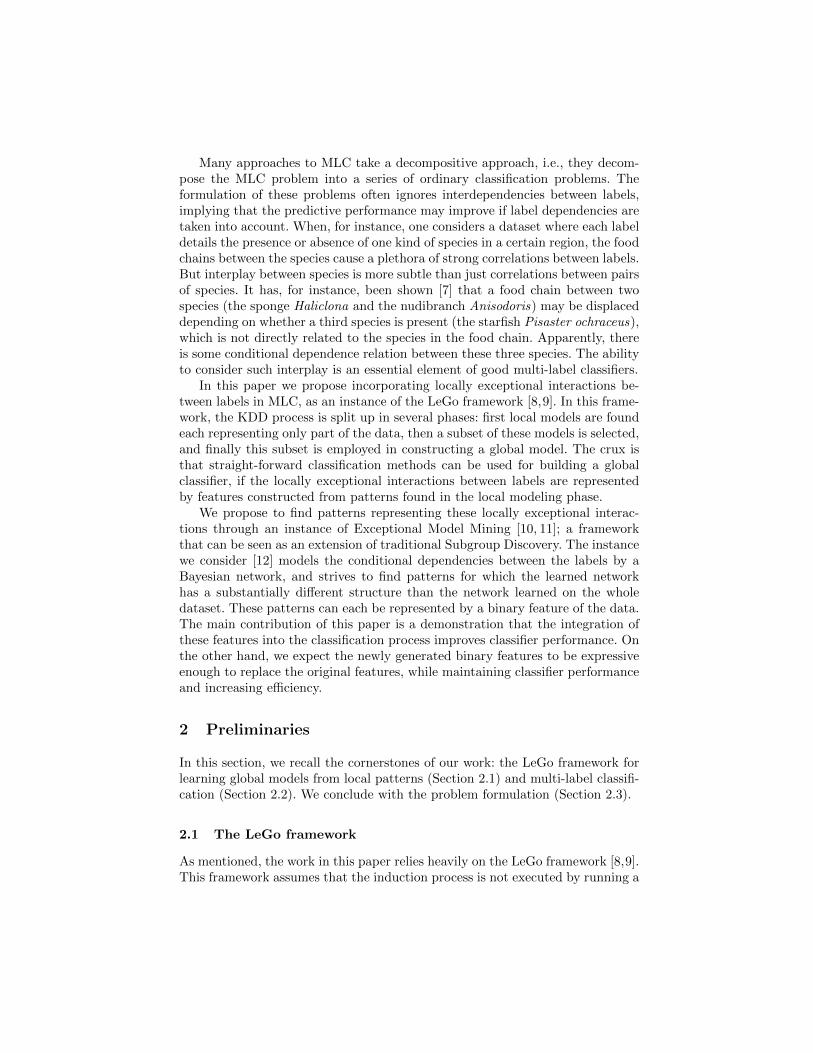
single learning algorithm, but rather consists of a number of consecutive phases,as illustrated in Figure 1. In the first phase a local pattern discovery algorithm isemployed in order to obtain a number of informative patterns, which can serveas relevant features to be used in the subsequent phases. These patterns canbe considered partial solutions to local complexities in the data. In the secondand third phase, the patterns are filtered to reduce redundancy, and the selectedpatterns are combined in a final global model, which is the outcome of theprocess.

The main reason to invest the additional computational cost of a LeGo ap-proach over a single-step algorithm, is the expected increase in accuracy of thefinal model, caused by the higher level of exploration involved in the initial lo-cal pattern discovery phase. Typically, global modeling techniques employ someform of greedy search, and in complex tasks, subtle interactions between at-tributes may be overlooked as a result of this. In most pattern mining methodshowever, extensive consideration of combinations of attributes is quite common.When employing such exploratory algorithms as a form of preprocessing, onecan think of the result (the patterns) as partial solutions to local complexities inthe data. The local patterns, which can be interpreted as new virtual features,still need to be combined into a global model, but potentially hard aspects of theoriginal representation will have been accounted for. As a result, straightforwardmethods such as Support Vector Machines with linear kernels can be used in theglobal modeling phase.

The LeGo approach has shown its value in a range of settings [8], particularlyregular binary classification [13,14], but we have specific reasons for choosing thisapproach in the context of multi-label classification (MLC). It is often mentionedthat in MLC, one needs to take into consideration potential interactions betweenthe labels, and that simultaneous classification of the labels may benefit fromknowledge about such interactions [15–18].

In [12], an algorithm was outlined finding local interactions amongst multipletargets (labels) by means of an Exceptional Model Mining (EMM) instance. TheEMM framework [11] suggests a discovery approach involving multiple targets,using local modeling over the targets in order to find subsets of the datasetwhere unusual (joint) target distributions can be observed. In [12], we presentedone instance of EMM that deals with discrete targets, and employs Bayesian

Attributes Labels ∈ 0, 1m

a11, . . . , a1k `11, . . . , `1m

.... . .

......

. . ....

an1 , . . . , ank `n1 , . . . , `nm

(a) input training set

Attributes Class ∈ La11, . . . , a

1k y11

.... . .

......

a11, . . . , a1k y1|Y1|

.... . .

......

(b) multiclass (MC)decomposition (onlyfor feature selection)

Attributes Class ∈ 2L

a11, . . . , a1k Y1

.... . .

......

an1 , . . . , ank Yn

(c) label powerset (LP) decom-position

Attributes Class1 ∈ 0, 1a11, . . . , a

1k `11

.... . .

......

an1 , . . . , ank `n1

· · ·

Attributes Classm ∈ 0, 1a11, . . . , a

1k `1m

.... . .

......

an1 , . . . , ank `nm

(d) binary relevance (BR) decomposition

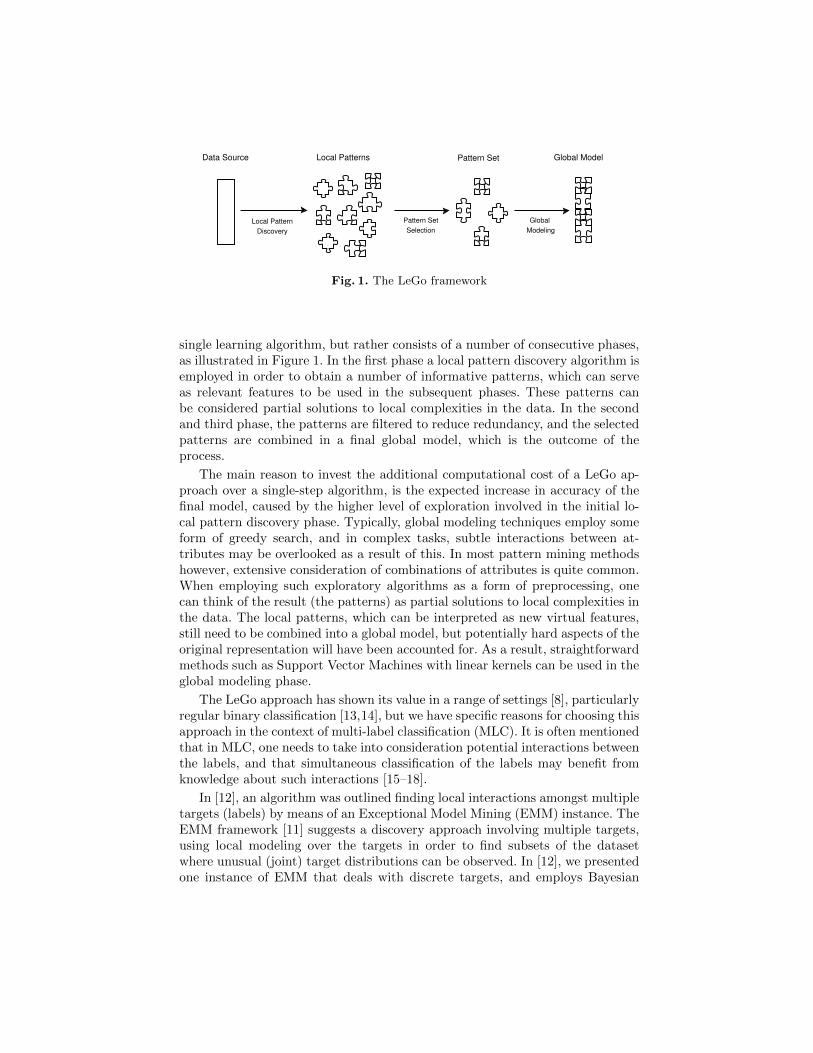
Fig. 2. Decomposition of multi-label training sets into binary (BR) or multiclass prob-lems (LP). Yi = yi1, . . . , yi|Yi|| y

ij ∈ L denotes the assigned labels `j | `ij = 1

to example xi. In LP the (single) target value of an instance xi is from the setYi| i = 1 . . .m ⊆ 2L of the different label subsets seen in the training data.

Networks in order to find patterns corresponding to unusual dependencies be-tween targets. This Bayesian EMM instance provides MLC with representationsof locally unusual combinations of labels.

2.2 Multi-label classification

Throughout this paper we assume a dataset Ω. This is a bag of N elements (datapoints) of the form x = a1, . . . , ak, `1, . . . , `m. We call a1, . . . , ak the attributesof x, and `1, . . . , `m ∈ L the labels of x. Each label `i is assumed to be discrete,and the vectors of attributes are taken from an unspecified domain A. Togetherwe call the attributes and labels of x the features of x. When necessary, wedistinguish the ith data point from other data points by adding a superscript ito the relevant symbols.

The task of multi-label classification (MLC) is, given a training set E ⊂ Ω,to learn a function f(a1, . . . , ak) → (`1, . . . , `m) which predicts the labels fora given example. Many multi-label learning techniques reduce this problem toordinary classification.

The widely used binary relevance (BR) [2, 3] approach tackles a multi-labelproblem by learning a separate classifier fi(a1, . . . , ak)→ `i for each label `i, asillustrated in Figure 2d. At query time, each binary classifier predicts whetherits class is relevant for the query example or not, resulting in a set of relevant

labels. Obviously, BR ignores possible interdependencies between classes since itlearns the relevance of each class independently.

One way of addressing this problem is by using classifier chains (CC) [17],which are able to model label dependencies since they stack the outputs of themodels: the prediction of the model for label `i depends on the predictions forlabels `1, . . . , `i−1. Hence, CC caters for dependencies of labels on multiple otherlabels, but these dependencies are one-directional: if label `i depends on theprediction for label `j , then `j does not depend on the prediction for `i.

An alternative approach is calibrated label ranking (CLR) [19], where the keyidea is to learn one classifier for each binary comparison of labels. CLR learnsbinary classifiers fij(a1, . . . , ak) → (`i `j), which predict for each label pair(`i, `j) whether `i is more likely to be relevant than `j . Thus, CLR (implicitly)takes correlations between pairs of labels into account. In addition, the decom-position into pairs of classes has the advantage of simpler sub-problems andhence commonly more accurately performing models [20]. Dependencies sharedbetween larger sets of labels are ignored by CLR.

Finally, a simple way to take label dependencies into account is the labelpowerset (LP) approach [2], treating each combination of labels occuring inthe training data as a separate value of a multi-class single-label classificationproblem (Figure 2c). Hence, LP caters for dependencies between larger sets oflabels as they appear in the dataset. However, LP disregards the inclusion latticethat exists between label sets in MLC. If data point x1 has label set `1, `2, anddata point x2 has label set `1, `2, `3, then the label set for x1 is a subset of thelabel set for x2. However, LP will represent these label sets as unrelated valuesof a single-label. So even though LP can cater for subtle label dependencies, thisinclusion information is not preserved.

We will use each of these techniques for decomposing a multi-label probleminto an ordinary classification problem in the third LeGo phase (Section 5).

2.3 Problem statement

The main question this paper addresses is whether a LeGo approach can improvemulti-label classification, compared to existing methods that do not employ apreliminary local pattern mining phase. Thus, our approach encompasses:

1. find a set P of patterns representing local anomalies in conditional depen-dence relations between labels, using the method introduced in [12];

2. filter out a meaningful subset S ⊆ P ;3. use the patterns in S as constructed attributes to enhance multi-label clas-

sification methods.

The following sections will explore what we do in each of these phases.

3 Local Pattern Discovery phase

To find the local patterns with which we will enhance the MLC attribute set,we employ an instance of Exceptional Model Mining (EMM). This instance is

tailored to find subgroups in the data where the conditional dependence relationsbetween a set of target features (our labels) is significantly different from thoserelations on the whole dataset. Before we recall the EMM instance in more detail,we will outline the general EMM framework.

3.1 Exceptional Model Mining

Exceptional Model Mining is a framework that can be considered an extensionof the traditional Subgroup Discovery (SD) framework, a supervised learningtask which strives to find patterns (defined on the input variables) that satisfya number of user-defined constraints. A pattern is a function p : A → 0, 1,which is said to cover a data point xi if and only if p

(ai1, . . . , a

ik

)= 1. We refer

to the set of data points covered by a pattern p as the subgroup correspondingto p. The size of a subgroup is the number of data points the correspondingpattern covers. The user-defined constraints typically include lower bounds onthe subgroup size and on the quality of the pattern, which is usually defined onthe output variables. A run of an SD algorithm results in a quality-ranked listof patterns satisfying the user-defined constraints.

In traditional SD, we have only a single target variable. The quality of a sub-group is typically gauged by weighing two factors: the size of the subgroup, andthe degree to which the distribution of the target within the subgroup deviatesfrom the target distribution on the whole dataset. EMM extends SD by allowingfor more complex target concepts defined on multiple target variables. It par-titions the features into two sets: the attributes and the labels. On the labelsa model class is defined, and an exceptionality measure ϕ for that model classis selected. Such a measure assigns a quality value ϕ(p) to a candidate patternp, based on model characteristics. EMM algorithms traverse a search lattice ofcandidate patterns, constructed on the attributes, in order to find patterns thathave exceptional values of ϕ on the labels.

3.2 Exceptional Model Mining meets Bayesian networks

As discussed in Section 2, we assume a partition of the k + m features in ourdataset into k attributes, which can be from any domain, and m labels, whichare assumed to be discrete. The EMM instance we employ [12] proposes to useBayesian networks (BNs) over those m labels as model class. These networks aredirected acyclic graphs (DAGs) that model the conditional dependence relationsbetween their nodes. A pattern has a model that is exceptional in this setting,when the conditional dependence relations between the m labels are significantlydifferent on the data covered by the pattern than on the whole dataset. Hencethe exceptionality measure needs to measure this difference. We will employ theWeighed Entropy and Edit Distance measure (denoted ϕweed), as introducedin [12]. This measure indicates the extent to which the BNs differ in structure.Because of the peculiarities of BNs, we cannot simply use traditional edit dis-tance between graphs [21] here. Instead, a variant of edit distance for BNs was

zx

y

(a)

zx

y

(b)

zx

y

(c)

zx

y

(d)

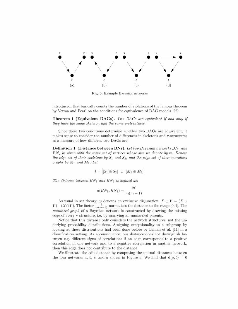
Fig. 3. Example Bayesian networks

introduced, that basically counts the number of violations of the famous theoremby Verma and Pearl on the conditions for equivalence of DAG models [22]:

Theorem 1 (Equivalent DAGs). Two DAGs are equivalent if and only ifthey have the same skeleton and the same v-structures.

Since these two conditions determine whether two DAGs are equivalent, itmakes sense to consider the number of differences in skeletons and v-structuresas a measure of how different two DAGs are.

Definition 1 (Distance between BNs). Let two Bayesian networks BN1 andBN2 be given with the same set of vertices whose size we denote by m. Denotethe edge set of their skeletons by S1 and S2, and the edge set of their moralizedgraphs by M1 and M2. Let

` =∣∣∣[S1 ⊕ S2] ∪ [M1 ⊕M2]

∣∣∣The distance between BN1 and BN2 is defined as:

d(BN1, BN2) =2`

m(m− 1)

As usual in set theory, ⊕ denotes an exclusive disjunction: X ⊕ Y = (X ∪Y )−(X∩Y ). The factor 2

m(m−1) normalizes the distance to the range [0, 1]. The

moralized graph of a Bayesian network is constructed by drawing the missingedge of every v-structure, i.e. by marrying all unmarried parents.

Notice that this distance only considers the network structures, not the un-derlying probability distributions. Assigning exceptionality to a subgroup bylooking at those distributions had been done before by Leman et al. [11] in aclassification setting. As a consequence, our distance does not distinguish be-tween e.g. different signs of correlation: if an edge corresponds to a positivecorrelation in one network and to a negative correlation in another network,then this edge does not contribute to the distance.

We illustrate the edit distance by computing the mutual distances betweenthe four networks a, b, c, and d shown in Figure 3. We find that d(a, b) = 0

and d(a, c) = d(a, d) = d(b, c) = d(b, d) = d(c, d) = 1/3. Only the two networksthat are equivalent have a distance of 0. If we compare the networks to theindependence model i which has no edges at all, we obtain d(a, i) = d(b, i) = 2/3,and d(c, i) = d(d, i) = 1.

This distance can now be used to quantify the exceptionality of a pattern; wedefine the quality measure edit distance (ϕed(p)) of pattern p to be the distancebetween the Bayesian network we fit on Ω (BNΩ) and the Bayesian network wefit on the subgroup corresponding to p (BNp), i.e. ϕed(p) = d(BNΩ , BNp).

Major changes in structure of the Bayesian networks are easily achieved ina small subset of the data. To counter this effect, the exceptionality measurewe employ also contains a component indicating the number of data points thepattern covers. We use the entropy (ϕent(p)) of the split between the patternand the rest of the dataset for this, capturing the information content of thesplit. It favours balanced splits over skewed splits, and again ranges between 0and 1, with the ends of the range reserved for the extreme cases (pattern beingempty or covering the whole dataset, and 50/50 splits, respectively).

Because we do not want to find patterns that have a low quality value oneither the edit distance or the entropy measure, we combine them into a weighedmeasure:

ϕweed(p) =√ϕent(p) · ϕed(p)

The original components ranged from 0 to 1, hence the Weighed Entropy andEdit Distance does so too. We take the square root of the entropy, reducing itsbias towards 50/50 splits, since we are primarily interested in a subgroup withlarge edit distance, while mediocre entropy is acceptable.

Notice that the EMM algorithm takes quite some time to complete: for eachcandidate pattern a Bayesian network is built over the labels, which can be donein O

(m2.376

)time [12]. Since many candidate patterns are considered, this is

a high price to pay, even with a relatively small number of labels. However,as stated in Section 2, in the LeGo approach the patterns resulting from theEMM algorithm can be considered partial solutions to local complexities in thedata. These solutions do not need to be recomputed every time a classifier isbuilt. Hence, the EMM algorithm needs to be executed only once, and we canafford to invest quite some computation time for this single run. Additionally,the investment needed to compare Bayesian networks as opposed to, for instance,comparing pairwise dependencies between labels, allows us to find anomalies innon-trivial interplay between variables. Such non-trivial modeling has proven itsworth in such diverse fields as marine biology [7], traffic accident reconstruction[23], medical expert systems [24], and financial operational risk [25].

After running the EMM algorithm, we obtain a set P of patterns each rep-resenting a local exceptionality in the conditional dependence relations betweenthe m labels, hence completing the Local Pattern Discovery phase.

4 Pattern Subset Discovery phase

Having outlined the details of local pattern discovery in a multi-label context,we now proceed to the second phase of the LeGo-framework: Pattern SubsetDiscovery. A common approach for feature subset selection for regular classifica-tion problems is to measure some type of correlation between a feature variableand the class variable. A subset of the features S from the whole set P is thendetermined either by selecting a predetermined number of best features or byselecting all features whose value exceeds a predetermined threshold. Unfortu-nately this approach is not directly applicable to multi-labeled data withoutadaptation. We experimented with the following approaches.

A simple way is to convert the multi-label problem into a multiclass (MC)classification problem, where each original instance is converted into several newinstances, one for each label `i assigned to the instance, using `i as the classvalue (see Figure 2b). However, this transformation does explicitly model labelco-occurence for a data point.

An alternative approach is to measure the correlations on the decomposedsubproblems produced by the binary relevance (BR) decomposition (see Figure2d). The m different correlation values for each feature are then aggregated. Inour experiments, we aggregated with the max operator, i.e., the overall relevancyof a feature was determined by its maximum relevance in one of the training setsof the binary relevance classifiers. The main drawback of this approach is that ittreats all labels independently and ignores that a feature might only be relevantfor a combination of class labels, but not for the individual labels.

The last approach employs the label powerset (LP) transformation (see Figure2c) in order to also measure the correlation of a feature to the simultaneousabsence or occurrence of label sets. Hence, with the dataset transformed into amulticlass problem, common features selection techniques can be applied. Thedifferent decomposition approaches are depicted in Figure 2.

After the transformations, we can use common attribute correlation measuresfor evaluating the importance of an attribute in each of the three approaches. Inparticular, we used the information gain and the chi-squared statistics value ofan attribute with respect to the class variable resulting from the decomposition,as shown in Figures 2b, 2d and 2c. Then we let each of the six feature selectionmethods select the best patterns from P to form the subset S. The size |S| ofthe subset is fixed in our experiments (see Section 5).

The approach adapted from multiclass classification of measuring the corre-lation between each feature and the class variable has known weaknesses such asbeing susceptible to redundancies within the features. Hence, in order to evaluatethe feature selection methods, we will compare them with the baseline methodthat simply draws S as a random sample from P .

5 Global Modeling phase

For the learning of the global multi-label classification models in the Global Mod-eling phase, we experiment with several standard approaches including binary

Attributes Labels

a11, . . . , a1k `11, . . . , `

1m

a21, . . . , a2k `21, . . . , `

2m

.... . .

......

. . ....

an1 , . . . , ank `n1 , . . . , `

nm

(a) input training set CO

Attributes Labels

p1(a11, . . . , a

1k

), . . . , p|S|

(a11, . . . , a

1k

)`11, . . . , `

1m

p1(a21, . . . , a

2k

), . . . , p|S|

(a21, . . . , a

2k

)`21, . . . , `

2m

.... . .

......

. . ....

p1 (an1 , . . . , ank ) , . . . , p|S| (a

n1 , . . . , a

nk ) `n1 , . . . , `

nm

(b) transformation into pattern space CS

Attributes Labels

a11, . . . , a1k, p1

(a11, . . . , a

1k

), . . . , p|S|

(a11, . . . , a

1k

)`11, . . . , `

1m

a21, . . . , a2k, p1

(a21, . . . , a

2k

), . . . , p|S|

(a21, . . . , a

2k

)`21, . . . , `

2m

.... . .

......

. . ....

.... . .

...

an1 , . . . , ank , p1 (an1 , . . . , a

nk ) , . . . , p|S| (a

n1 , . . . , a

nk ) `n1 , . . . , `

nm

(c) combined attributes in the LeGo classifier CL

Fig. 4. A multi-label classification problem (a), its representation in pattern space (b)given the set of patterns p1, . . . , p|S|, and the LeGo combination (c)

relevance (BR) and label powerset (LP) decompositions [2,3], as well as a selec-tion of effective recent state-of-the-art learners such as calibrated label ranking(CLR) [19, 26], and classifier chains (CC) [17]. The chosen algorithms cover awide range of different approaches and techniques used for learning multi-labelproblems (see Section 2.2), and are all included in Mulan, an excellent libraryfor multi-label classification algorithms [2, 27].

We combine the multi-label decomposition methods mentioned in Section 5with several base learners: J48 with default settings [28], standard LibSVM [29],and LibSVM with a grid search on the parameters. In this last approach, mul-tiple values for the SVM kernel parameters are tried, and the one with the best3-fold cross-validation accuracy is selected for learning on the training set (assuggested by [29]). Both SVM methods are run once with the Gaussian RadialBasis Function as kernel, and once with a linear kernel using the efficient Lib-Linear implementation [30]. We will refer to LibSVM with the parameter gridsearch as MetaLibSVM, and denote the used kernel by a superscript rbf or lin.

For each classifier configuration, we learn three classifiers based on differentattribute sets. The first classifier uses only the k attributes that make up theoriginal dataset, and is denoted CO (Figure 4a). The second classifier, denotedCS , uses only attributes constructed from our pattern set S. Each of these pat-terns by definition maps each record in the original dataset to either zero or one.Hence they can be trivially transformed into binary attribute, that together makeup the attribute space for classifier CS (Figure 4b). The third classifier employsboth the k original and |S| constructed attributes, in the spirit of LeGo, andis hence denoted CL (Figure 4c). Its attribute space consists of the k original

Table 1. Datasets used in the experiments, shown with the number of examples (N),attributes (k), and labels (m), as well as the average number of labels per example

Dataset Domain N k m Cardinality

Emotions Music 593 72 6 1.87Scene Vision 2407 294 6 1.07Yeast Biology 2417 103 14 4.24

attributes, and |S| attributes constructed from the pattern set S for a grandtotal of k + |S| attributes.

6 Experimental setup

To experimentally validate the outlined LeGo method, we will compare the per-formance of the three classifiers based on different attribute sets CO, CS , andCL. We will also investigate the relative performance of the different featureselection methods, and the relative performance of classification approaches.

6.1 Experimental procedure

For the experiments we selected three multi-labeled datasets from different do-mains. Statistics on these datasets can be found in Table 1. The column Cardi-nality displays the average number of relevant labels for a data point.

The Emotions dataset [4] consists of 593 songs, from which 8 rhythmicand 64 timbre attributes were extracted. Domain experts assigned the songsto any number of six main emotional clusters: amazed-surprised, happy-pleased,relaxing-calm, quiet-still, sad-lonely, and angry-fearful.

The Scene dataset [5] is from the semantic scene classification domain, inwhich a photo can be classified into one or more of 6 classes. It contains 2407photos, each of which is divided in 49 blocks using a 7× 7 grid. For each blockthe first two spatial color moments of each band of the LUV color space arecomputed. This space identifies a color by its lightness (the L* band) and twochromatic valences (the u* and v* band). The photos can have the classes beach,field, fall foliage, mountain, sunset, and urban.

From the biological field we consider the Yeast dataset [6]. It consists ofmicro-array expression data and phylogenetic profiles with 2417 genes of theyeast Saccharomyces cerevisiae. Each gene is annotated with any number of 14functional classes.

All statistics on the classification processes are estimated via a 10-fold cross-validation. To enable a fair comparison of the LeGo classifier with the otherclassifiers, we let the entire learning process consider only the training set foreach fold. This means that we have to run the Local Pattern Discovery andPattern Subset Discovery phase separately for each fold.

For every fold on every dataset, we determine the best 10,000 patterns, (ifno 10,000 patterns can be found, we report them all), measuring the exception-ality with ϕweed as described in Section 3.2. The search space in EMM cannotbe explored exhaustively when there are numerical attributes and a nontrivialquality measure, and both are the case here. Hence we resort to a beam searchstrategy, configured with a beam width of w = 10 and a maximum search levelof 2 (for more details on beam search in EMM, see [12]). We specifically selecta search of modest depth, in order to prevent producing an abundance of highlysimilar patterns. We further bound the search by setting the minimal coverageof a pattern at 10% of the dataset.

Notice that the choice of search lattice traversal does not influence the waythe exceptionality measure determines the quality of a pattern. While settingthe search depth to 2 does influence the complexity of the pattern in attributespace, this setting is independent from the complexity of the models we fit in labelspace. Each candidate pattern will be evaluated by fitting a Bayesian networkto all its labels, regardless of search parameters such as the search depth.

For each dataset for each fold, we train classifiers from the three trainingsets CO, CS , and CL for each combination of a decomposition approach andbase learner. We randomly select |S| = k patterns (cf. Section 5), i.e. exactly asmany pattern-based attributes for CS and CL as there are original attributes inCO.

6.2 Evaluation measures

We evaluate the effectiveness of the three classifiers for each combination on therespective test sets for each fold with five measures: Micro-Averaged Precisionand Recall, Subset Accuracy, Ranking Loss, and Average Precision (for detailson computation cf. [19] and [2]). We define Yi =

`j | `ij = 1

as the set of

assigned labels and Yi as the set of predicted labels for a test instance xi. Wefind these five measures a well balanced selection from the vast set of multi-labelmeasures, evaluating different aspects of multi-label predictions such as goodranking performance and correct bipartition.

From a confusion matrix aggregated over all labels and examples, Precision(Prec) computes the percentage of predicted labels that are relevant, and Recall(Rec) computes the percentage of relevant labels that are predicted. Recalland precision allow a commensurate evaluation of an algorithm, in contrast toHamming loss, which is often used but unfortunately generally favors algorithmswith high precision and low recall.

Prec =

∑i

∣∣∣Yi ∩ Yi∣∣∣∑i

∣∣∣Yi∣∣∣ Rec =

∑i

∣∣∣Yi ∩ Yi∣∣∣∑i |Yi|

Subset Accuracy (Acc) denotes the percentage of perfectly predicted labelsets, basically forming a multi-label version of traditional accuracy.

Acc =

∑i I[Yi = Yi

]∑i 1

, I[x] =

1 if x is true

0 otherwise

Since the classifiers we consider are able to return rankings on the labels, wealso computed the following rank-based loss measures, in which r(`) returningthe position of label `. Ranking Loss (Rank) returns the number of pairs oflabels which are not correctly ordered, normalized by the total number of pairs.

Rank =|(` ∈ Y, `′ /∈ Y) | r(`) < r(`′)|

|Y| · (m− |Y|)

Average Precision (AvgP) computes the precision at each relevant label inthe ranking, and averages these percentages over all relevant labels.

AvgP =1

|Y|∑`∈Y

|`′ ∈ Y | r(`′) ≤ r(`)|r(`)

These two ranking measures are computed for each example and then averagedover all examples.

All values for all settings are averaged over the folds of the cross-validation.Thus we obtain 300 test cases (5 evaluation measures × 5 base learners × 4decomposition approaches × 3 datasets).

6.3 Statistical testing

To draw conclusions from the long list of raw results we obtained, we use themethodology for the comparison of multiple algorithms described by Demsar [31].First, we perform a Friedman test [32,33] to determine whether the classifiers allperform similarly. This is a non-parametric equivalent of the repeated-measuresANOVA. For each test case we rank the classifiers by their performance. Let Tdenote the number of test cases, and let rj be the average rank over all test casesfor classifier Cj , where j ∈ O,S, L. Whenever a tie occurs, average ranks areassigned. The null hypothesis now states that all classifiers perform equivalentlyand so their average ranks should be equal. Under this null hypothesis, theFriedman statistic

χ2F =

12T

g(g + 1)·∑j

(rj −

g + 1

2

)2

has a chi-squared distribution with g− 1 degrees of freedom, when N and k aresufficiently large. Here, g denotes the number of classifiers we are comparing.3

3 notice that while Demsar gives a different equation for the Friedman statistic, thisis the equation given by Friedman himself. Equivalence can be shown in four lines ofmath; the equation shown here is slightly easier to compute, and easier on the eye.

Table 2. Average ranks of different feature selection methods, with critical difference

Selection method BR LP MC Random CDEvaluation method χ2 gain χ2 gain χ2 gain

Rank 4.445 3.932 3.507 4.263 3.707 4.490 3.657 0.520

If the null hypothesis is rejected, we can determine which classifiers are sig-nificantly better than others with a post-hoc test. As proposed by Demsar, weuse the Nemenyi test [34], which is similar to the Tukey test for ANOVA. Thetest entails that the performance of two classifiers is significantly different if thedifference between their average ranks is at least the critical difference:

CD = qα

√g(g + 1)

6T

where qα are critical values based on the Studentized range statistic divided by√2. Finally and quite obviously, if the Nemenyi test yields that two classifiers

have significantly different performance, the one with the better overall rankperforms significantly better.

7 Experimental evaluation

The following subsections are dedicated to different aspects such as as the eval-uation of the different pattern subset discovery approaches, the employment ofthe different attribute sets, the impact of the decomposition approaches, andefficiency.

7.1 Feature selection methods

Before comparing the three classifiers, we take a look at the relative performanceof the different feature selection methods. When comparing the performance ofthe classifier CL with different feature selection methods over all T = 300 testcases, we find the average ranks in Table 2. We compared the Binary Relevance,Label Powerset and MultiClass approach, each with evaluation measures chi-squared and information gain, and the random baseline approach.

The results show that no classifier employing a sophisticated feature selectionmethod significantly4 outperforms the classifier with random feature selection.

4 Since we are comparing g = 7 different methods here, the critical value with sig-nificance level α = 5% for the chi-squared distribution with g − 1 = 6 degrees offreedom equals 12.592. The Friedman statistic for these ranks equals χ2

F = 61.678,hence the Friedman test is passed. For the Nemenyi test, when comparing 7 meth-ods, the critical value is q0.05 = 2.948. Hence the critical difference between averageranks becomes CD = 0.520.

Conversely, this classifier does significantly outperform several classifiers em-ploying sophisticated feature selection. For the binary relevance and multiclassapproaches this is reasonable, since the patterns are explicitly designed to con-sider interdependencies between labels, while the BR and MC approaches selectfeatures based on their correlation with single labels only and hence ignore in-terdependencies. The label powerset approach should do better in this respect.In fact, the best average rank featured in Table 2 belongs to LP with the chi-squared evaluation measure. Since its improvement over the naive method is notsignificant, we did not further explore its performance, but that does not meanit is without merit.

Another reason for the bad performance of the feature selection methods isthat they evaluate each feature individually. One extreme use case will show theproblem: if we replicate each feature n times and we select the n best featuresaccording to the presented methods, we will get n times the same (best) feature.In the Local Pattern Mining phase, we produce a high number of additionalfeatures, hence we can expect to obtain groups of similar additional featureswhere this problem may appear. The random feature selection does not sufferfrom this problem. As a result of these experiments, we decided not to use anysophisticated feature selection in the remaining experiments, and focus on theresults for random feature selection.

7.2 Evaluation of the LeGo approach

The first row in Table 3 compares the three different representations CO, CS ,and CL over the grand total of 300 test cases in terms of average ranks. Wesee that both CO and CL perform significantly (α = 5%)5 better than CS ,i.e. the pattern-only classifier cannot compete with the original attributes orthe combined classifier. The difference in performance between CO and CL isnot significant. Although the average rank for the LeGo-based classifier is some-what higher, we cannot claim that adding local patterns leads to a significantimprovement. The remainder of Table 3 is concerned with stratified results.

When stratifying the results by base learner (the second block in Table 3),we notice a striking difference in average ranks between J48 and the rest. Whenwe restrict ourselves to the results obtained with J48, we find that rO = 1.433,rS = 2.517, and rL = 2.050, with CD = 0.428. Here, the classifier built fromoriginal attributes significantly (α = 5%) outperforms the LeGo classifier.

One reason for the performance gap between J48 and the SVM approachlies in the way these approaches construct their decision boundary. The SVMapproaches draw one hyperplane through the attribute space, whereas J48 con-structs a decision tree, which corresponds to a decision boundary consisting of

5 Since we are comparing three classifiers, the Friedman statistic equals χ2F = 52.687.

With significance level α = 5%, the critical value for the chi-squared distributionwith 2 degrees of freedom equals 5.991, hence the null hypothesis of the Friedmantest is comfortably rejected. For the post-hoc Nemenyi test, when comparing threeclassifiers the critical value is q0.05 = 2.344. Hence, the critical difference betweenaverage ranks becomes CD = 0.191, with significance level α = 5%.

Table 3. Comparison of different attribute sets. Average ranks of the three classifiersCO, CS , CL, with critical difference, over all 300 test cases, over all 240 test casesbarring J48, over all 60 test cases with a particular base learner, and over all 75 testcases with a particular decomposition method. Bold numbers indicates the top rank inthe row, > or < indicate a significant difference to the direct neighbor classifier.

CO CL CS CD

Overall 1.863 = 1.797 > 2.340 0.191Without J48 1.971 < 1.733 > 2.296 0.214

MetaLibSVMrbf 1.483 = 1.683 > 2.833 0.428

MetaLibSVMlin 1.900 = 1.800 > 2.300 ”

LibSVMrbf 2.633 < 1.683 = 1.683 ”

LibSVMlin 1.867 = 1.767 > 2.367 ”J48 1.433 > 2.050 > 2.517 ”

Acc 1.850 = 1.800 > 2.350 ”Prec 1.700 = 1.883 > 2.417 ”Rec 1.983 = 1.700 > 2.317 ”AvgP 1.850 = 1.833 > 2.317 0.428Rank 1.933 = 1.767 > 2.300 ”

CLR 1.813 = 1.760 > 2.427 0.383LP 1.773 = 1.827 > 2.400 ”CC 1.947 = 1.720 > 2.333 ”BR 1.920 = 1.880 = 2.200 ”

Emotions 2.510 < 1.860 = 1.630 0.331Scene 1.480 = 1.640 > 2.880 ”Yeast 1.600 = 1.890 > 2.510 ”

axis-parallel fragments. The patterns the EMM algorithm finds in the Local Pat-tern Discovery phase are constructed by several conditions on single attributes.Hence the domain of each pattern has a shape similar to a J48 decision boundary,unlike a (non-degenerate) SVM decision boundary. Hence, the expected perfor-mance gain when adding such local patterns to the attribute space is much higherfor the SVM approaches than for the J48 approach.

Using only the original attributes seems to be enough for the highly optimizednon-linear MetaLibSVMrbf method, though the difference to the combined at-tributes is small and not statistically significant. The remaining base learnersbenefit from the additional local patterns. Notably, when using LibSVMrbf, it iseven possible to rely only on the pattern-based attributes in order to outperformthe classifiers trained on the original attributes.

Because the J48 approach results in such deviating ranks, we investigate therelative performance of the base learners. We compare their performance on thethree classifiers CO, CS , and CL, with decomposition methods BR, CC, CLR,and LP, on the datasets from Table 1, evaluated with the measures introducedin Section 6.1. The average ranks of the base learners over these 180 test casescan be found in Table 4; Again, the Friedman test is easily passed. The Nemenyitest shows that J48 performs significantly worse than all SVM methods and that

MetaLibSVMrbf clearly dominates the performance of the SVMs. This last pointis not surprising, since the three datasets are known to be difficult and hencenot linearly separable [19], which means that an advantage of the RBF-kernelover the linear kernel can be expected. Moreover, the non expensively optimizedLibSVMrbf can be considered to be subsumed by the meta variant since the gridsearch includes the default settings.

Having just established that J48 is the worst-performing base learner and,additionally, that the similar decision patterns particularly damage the perfor-mance of the LeGo classifier, we repeat our overall comparison considering onlythe SVM variants. Moreover, SVMs are conceptually different from decision treelearners, which additionally justifies the separate comparison. The average ranksof the three classifiers CO, CS , and CL on the remaining 240 test cases can befound in the second row of Table 3. This time, the Nemenyi test yields that onthe SVM methods the LeGo classifier is generally significantly better than theclassifier built from original attributes, even though for MetaLibSVMrbf this isnot the case.

When stratifying the results by quality measure (the third block in Table 3)we find that the results are consistent over the chosen measures. For all measureswe find that CL significantly outperforms CS , and CO always outperforms CSthough not always significantly. Additionally, for all measures except precision,CL outranks CO, albeit non-significantly. This consistency provides evidence forrobustness of the LeGo method.

The fourth block in Table 3 concerns the results stratified by transformationtechnique. With the exception of the label powerset approach, which by itselfrespects relatively complex label dependencies, all approaches benefit from thecombination with the constructed LeGo attributes, though the differences arenot statistically significant. Of peculiar interest is the benefit for the binaryrelevance approach, which in its original form considers each label independently.Though the Friedman test is not passed, the trend is confirmed by the resultsof CC, which additionally include attributes from the preceding base classifiers’predictions.

As stated in Section 2.2, to predict label `i the CC decomposition approachallows using the predictions made for labels `1, . . . , `i−1. Hence we can view CCas an attribute enriching approach, adding an attribute set C. The result com-paring the performance of the different attribute sets arrives at O ∪S ∪C (rank2.84) followed by O ∪ S (3.34), O ∪C (3.53), O (3.6), S (3.89) and S ∪C (3.97)(significant difference only between first and both last combinations). Hence,adding C has a similar effect on performance than adding S, and BR particu-larly benefits if both are added, which demonstrates that the patterns based onlocal exceptionalities provide additional information on the label dependencieswhich is not covered by C.

In the last block of Table 3 we see that results vary wildly when stratifiedby dataset. We see no immediate reason why this should be the case; perhaps astudy involving more datasets could be fruitful in this respect.

Table 4. Average ranks of the base learners, with critical difference CD

Approach MetaLibSVMrbf MetaLibSVMlin LibSVMlin LibSVMrbf J48 CD

Rank 1.489 2.972 3.228 3.417 3.894 0.455

Table 5. Comparison of the decomposition approaches. The first block compares theapproaches for all base learner combinations, the second one restricts on the usage ofMetaLibSVMrbf. The first row in each block indicates the average ranks with respectto all evaluation metrics, whereas the following rows distinguish between the individualmeasures.

Measure CLR LP CC BR CD

all & all BC 1.909 > 2.462 = 2.700 = 2.929 0.313Acc 3.400 < 1.489 = 1.722 > 3.389 0.700Prec 1.989 > 3.467 = 3.111 < 1.433 ”Rec 2.156 = 1.956 = 2.422 > 3.467 ”AvgP 1.000 > 2.778 = 3.111 = 3.111 ”Rank 1.000 > 2.622 = 3.133 = 3.244 ”

all & MetaLibSVMrbf 2.111 = 1.911 > 2.911 = 3.067 0.700Acc 3.667 < 1.000 = 2.000 = 3.333 1.563Prec 2.111 = 3.444 = 3.444 < 1.000 ”Rec 2.778 < 1.000 = 2.333 = 3.889 ”AvgP 1.000 = 2.111 = 3.444 = 3.444 ”Rank 1.000 = 2.000 = 3.333 = 3.667 ”

7.3 Evaluation of the decompositive approaches

We can learn more from Table 3 when more blocks are additionally stratified byevaluation measure. Indeed, the decision of the feature base does not seem tohave a differing impact on the metrics (for the SVM learners, not shown in thetable). The only exception appears to be micro-averaged precision, for which COyields a small advantage over CL. But as Table 5 demonstrates, the situationchanges with respect to the decompositive approach used. As we can see in theupper block, there are clear tendencies regarding the preference for a particularmetric.

For instance, LP has a clear advantage in terms of subset accuracy, whichonly CC is able to approximate. This is natural, since both approaches are ded-icated to the prediction of a correct labelset. In fact, LP only predicts labelsetspreviously seen in the training data. CC behaves similarly, as is shown in thefollowing: if we consider only the additional attributes from the previous predic-tions (i.e. attribute set C), then we found that CC behaves similar to a sequencetagger. Hence, for a particular sequence of labels `1, . . . , `i−1 the i-th classifierin the chain will tend to predict `i = 1 (or `i = 0 respectively) only if `1, . . . , `iexisted in the training data. The advantage of LP and CC is confirmed in the

bottom block, which restricts the comparison to the usage of the most accuratebase learner MetaLibSVMrbf.

Precision is dominated by BR, followed by CLR. This result is obtainedby being very cautious at prediction, as the values for recall show. Especiallythe highly optimized SVM is apparently fitted towards predicting a label onlyif it is very confident that the estimation is correct. It is not clear whetherthis is due to the high imbalance of the binary subproblems, e.g. compared topairwise decomposition. CLR shows to be more robust, though a bias towardsunderestimating the size of the label sets is visible. Especially in this case thebias may originate from the conservative BR classifiers, which are included in thecalibrated ensemble, since the difference between precision and recall is clearlyhigher for MetaLibSVMrbf.

A contrary behavior to BR is shown by LP, which dominates recall, espe-cially for MetaLibSVMrbf, but completely neglects precision. This indicates apreference for predicting the more rare large labelsets. The best balance betweenprecision and recall is shown by CLR. Even for MetaLibSVMrbf, for which theunderestimation leads to low recall, but for which the competing classifier chainsobtain the worst precision values together with LP.

The good balancing properties of CLR are confirmed by the results on theranking losses, which are clearly dominated by CLR’s good ability to produce ahigh density of relevant labels at the top of the the rankings. The high recall of LPcorresponds with good ranking losses, but the low ranks of BR demonstrate thatits high precision is not due to a good ranking ability. This behavior was alreadyobserved e.g. in [19] and [20] where BR often correctly pushed a relevant classat the top, but obtained poor ranking losses. Similarly, CC’s base classifiers aretrained independently without a common basis for confidence scores and henceachieve a low ranking quality.

If we give the same weight to the five selected measures, we observe that CLRsignificantly outperforms the second placed LP if all base learner are considered,and slightly loses against LP if MetaLibSVMrbf is used (top row in both blocksin Table 3).

7.4 Efficiency

Apart from the unsatisfactory performance of the J48 approach compared toSVM approaches, Table 4 also indicates that compared to the standard LibSVMapproach, the extra computation time invested in the MetaLibSVM parametergrid search is rewarded with a significant increase in classifier performance. Forboth the linear and the RBF kernel we see that the MetaLibSVM approachoutperforms the LibSVM approach, although this difference is only significant forthe RBF kernel. A more exhaustive parameter-optimizing search will probablybe beneficial, since the grid search considers arbitrary parameter values. Whetherthe performance increase is worth the invested time is a question of preference.In the case where time and computing power are not limited resources, theincreased performance is clearly worthwhile.

From a practical point of view, it is also interesting to analyze the efficiencyof using the original attributes in comparison to using the constructed attributes.We expected an improvement in complexity just from the fact that the patternattributes are binary in contrast to the more complex nature of the originalattributes in the used datasets. In addition, it is well known that the possi-bly resulting sparseness of the binary attributes may also boost algorithms likeSVMs.

For the comparison between training of CO and CS we focus on the BinaryRelevance decomposition setting in order to allow a balanced comparison overthe three datasets, since the complexity of BR scales linearly with respect to thenumber of classes. For J48 as base learner, we observed a reduction of trainingcosts from 28% (Emotions) over 31% (Scene) to 47% for Yeast. For LibSVMrbf,the difference was more pronounced, with a reduction of 60%, 52% and 50%,resp. We obtained a similar picture for LibSVMlin, with a reduction of even 82%(Emotions) and 65% (Scene), except for Yeast, where training CS surprisinglytakes almost 7 times longer than training CO. This case is very likely an exceptionsince comparing LibSVMlin and hence using different parameters shows againa clear reduction. The numbers for MetaLibSVMlin and MetaLibSVMrbf areomitted since they show a similar picture but are more difficult to comparedirectly since they always also include testing time.

Note that training CL of course takes more computation time since we employboth attribute sets, but the overhead of using the constructed attributes fromthe patterns is clearly relatively small. Also, notice that the overhead needs tobe invested only once for training the classifier, possibly off-line, and that theresulting trained classifier can then be used again and again for classifying data;if one wants to classify more than once, the added complexity diminishes.

8 Discussion and related work

In traditional subgroup discovery, it is common to traverse the search space ex-haustively [35, 36]. Usually the assumption is made that all attributes of thedataset are nominal. Most current work on subgroup discovery still incorpo-rates this restriction [37], but recently subgroup discovery on numeric domainshas received more attention [38]. In this work the search space is traversed ex-haustively even though it contains numeric attributes. However, this can onlybe done under the restriction that the employed quality measure has a certainanti-monotonic property: if one could compute an optimistic estimate for thequality of any refinement of a given candidate pattern, the search space can besignificantly pruned.

Conversely, we choose to let our work be free from the restrictions of nomi-nality of the datasets and anti-monotonicity of the quality measure, since manyreal-life datasets contain numeric attributes and we expect to benefit from usinga more complex quality measure. We also expect little disadvantage from usingheuristic rather than exhaustive search in the Local Pattern Discovery phase.The found patterns are afterwards put through the Pattern Subset Discovery

phase, where they are subjected to feature selection which is heuristic by def-inition, hence there is really no point in enforcing an exhaustive search in theLocal Pattern Discovery phase.

The applied Local Pattern Discovery algorithm was created to find patternsthat are interesting by themselves. The output of the algorithm is thereforenot specifically tailored to be useful in a classification setting; this is not aguiding principle in the Exceptional Model Mining process. To the best of ourknowledge, this work is a first shot at testing the utility for classification of theresult of such a stand-alone multi-label pattern discovery process. Some recentsophisticated classifiers, for instance the multi-label lazy associative classifiers[39], are also based on local patterns. However, these patterns serve only theclassifier, hence the different phases, as present in the LeGo framework, are notas separated as they are in our work. Similarly, Cheng and Hullermeier [15]incorporate additional attributes that encode the label distribution in the directneighborhood by, in effect, stacking the output of a k-Nearest Neighbor classifier.However, this has to be done at (training and testing) runtime and cannot bedone separately and beforehand.

Other known stacking approaches include the outcome of global classifiers.Godbole and Sarawagi [40] use the outputs of a BR-SVM classifier as addi-tional input attributes for second-level SVMs. Similarly, Tsoumakas et al. [41]replace all original attributes by the predicted scores of a BR. The scores areadditionally filtered according to their correlation to each other. The employedclassifier chains [17] rely on stacking the outcomes of the predetermined sequenceof previous binary relevance classifiers, which permits to model conditional de-pendencies, but it does not rely on locality. Zhang and Zhang [18] also try tomodel label dependencies and start from the premise of eliminating the condi-tional dependency between the input attributes a1, . . . , ak and the individuallabels by computing the errors ei as difference between true label `i and the pre-diction. The isolated dependencies between labels are then approximated by theresult of building a Bayesian network on these errors. A new BR classifier is thenlearned for each class with the set of alleged parents as additional attributes.The very recent LIFT algorithm selects particularly representative centroids inthe positive and negative examples of a class by k-means clustering and thenreplaces the original attributes of an instance by the distances to these repre-sentatives [42]. One may also interpret this approach as a different, pragmaticway of computing new suitable principal components and hence dimensionalityreduction, which apparently works quite well.

9 Conclusions

We have proposed enhancing multi-label classification methods with local pat-terns in a LeGo setting. These patterns are found through an instance of Ex-ceptional Model Mining, a generalization of Subgroup Discovery striving to findsubsets of the data with aberrant conditional dependence relations between tar-get features. Hence each pattern delivered represents a local anomaly in con-

ditional dependence relations between targets. Each pattern corresponds to abinary attribute which we add to the dataset, to improve classifier performance.

Experiments on three datasets show that for multi-label SVM classifiers theperformance of the LeGo approach is significantly better than the traditionalclassification performance: investing extra time in running the EMM algorithmpays off when the resulting patterns are used as constructed attributes. TheJ48 classifier does not benefit from the local pattern addition, which can be at-tributed to the similarity of the local decision boundaries produced by the EMMalgorithm to those produced by the decision tree learner. Hence the expectedperformance gain when adding local patterns is lower for J48 than for approachesthat learn different types of decision boundaries, such as SVM approaches.

The Friedman-Nemenyi analysis also shows that the constructed attributesgenerally cannot replace the original attributes without significant loss in clas-sification performance. We find this reasonable, since these attributes are con-structed from patterns found by a search process that is not at all concernedwith the potential of the patterns for classification, but is focused on exception-ality. In fact, the pattern set may be highly redundant. Additionally it is likelythat the less exceptional part of the data, which by definition is the majority ofthe dataset, is underrepresented by the constructed attributes.

To the best of our knowledge, this is a first shot at discovering multi-labelpatterns and testing their utility for classification in a LeGo setting. Thereforethis work can be extended in various ways. It might be interesting to developmore efficient techniques without losing performance. One could also exploreother quality measures, such as the plain edit distance measure from [12], orother search strategies. In particular, optimizing the beam-search in order toproperly balance its levels of exploration and exploitation, could fruitfully pro-duce a more diverse set of attributes [43] in the Local Pattern Discovery phase.Alternatively, pattern diversity could be addressed in the Pattern Subset Selec-tion phase, ensuring diversity within the subset S rather than enforcing diversityover the whole pattern set P .

As future work, we would like to expand our evaluation of these methods.Recently, it has been suggested that for multi-label classification, it is better touse stratified sampling than random sampling when cross-validating [44]. Also,experimentation on more datasets seems prudent. In this paper, we have exper-imented on merely three datasets, selected for having a relatively low number oflabels. As stated in Section 3.2, we have to fit a Bayesian network on the labelsfor each subgroup under consideration, which is a computationally expensive op-eration. The availability of more datasets with not too many labels (say, m < 50)would allow for more thorough empirical evaluation, especially since it would al-low us to draw potentially significant conclusions from Friedman and Nemenyitests per evaluation measure per base classifier per decomposition scheme. Withthree datasets this would be impossible, so we elected to aggregate all thesetest cases in one big test. The observed consistent results over all evaluationmeasures provide evidence that this aggregation is not completely wrong, buttheoretically this violates the assumption of the tests that all test cases are inde-

pendent. Therefore, the empirically drawn conclusions in this paper should notbe taken as irrefutable proof, but more as evidence contributing to our beliefs.

Acknowledgments This research is financially supported by the Netherlands Organi-

sation for Scientific Research (NWO) under project number 612.065.822 (Exceptional

Model Mining) and by the German Science Foundation (DFG). We also gratefully

acknowledge support by the Frankfurt Center for Scientific Computing.

References

1. W. Duivesteijn, E. Loza Mencıa, J. Furnkranz, A. Knobbe, Multi-label LeGo— Enhancing Multi-label Classifiers with Local Patterns, Advances in Intelli-gent Data Analysis XI – 11th International Symposium, IDA 2012, Helsinki, Fin-land, October 25-27, 2012, Proceedings. LNAI 7619, pp. 114-125, 2012. http:

//www.ke.tu-darmstadt.de/publications/papers/IDA-12.pdf.2. G. Tsoumakas, I. Katakis, I. P. Vlahavas, Mining Multi-label Data, Data Mining

and Knowledge Discovery Handbook, Springer, pp. 667–685, 2010.3. G. Tsoumakas, I. Katakis, Multi-Label Classification: An Overview, International

Journal of Data Warehousing and Mining 3 (3), pp. 1–13, 2007.4. K. Trohidis, G. Tsoumakas, G. Kalliris, I. P. Vlahavas, Multi-Label Classification

of Music into Emotions, Proc. 9th International Conference on Music InformationRetrieval, pp. 325–330, 2008.

5. M. R. Boutell, J. Luo, X. Shen, C. M. Brown, Learning Multi-Label Scene Classi-fication, Pattern Recognition 37 (9), pp. 1757–1771, 2004.

6. A. Elisseeff, J. Weston, A Kernel Method for Multi-Labelled Classification, Ad-vances in Neural Information Processing Systems 14, pp. 681–687, MIT Press,Cambridge MA, 2002.

7. R. T. Paine, Food Web Complexity and Species Diversity, The American Naturalist100 (910), pp. 65–75, 1966.

8. J. Furnkranz, A. Knobbe (eds.), Special Issue: Global Modeling Using Local Pat-terns, Data Mining and Knowledge Discovery journal 20 (1), 2010.

9. A. Knobbe, B. Cremilleux, J. Furnkranz, M. Scholz, From local patterns to globalmodels: The LeGo approach to data mining, Proc. ECMLPKDD’08 WS FromLocal Patterns to Global Models, pp. 1–16, 2008.

10. M. van Leeuwen, Maximal Exceptions with Minimal Descriptions, Data Miningand Knowledge Discovery journal, special issue ECMLPKDD’10, 21 (2), pp. 259–276, Springer, 2010.

11. D. Leman, A. Feelders, A. Knobbe, Exceptional Model Mining, Proc.ECML/PKDD (2), pp. 1–16, 2008.

12. W. Duivesteijn, A. Knobbe, A. Feelders, M. van Leeuwen, Subgroup Discoverymeets Bayesian networks – an Exceptional Model Mining approach, Proc. ICDM,pp. 158–167, 2010.

13. A. Knobbe, J. Valkonet, Building Classifiers from Pattern Teams, From LocalPatterns to Global Models: Proc. ECML PKDD 2009 Workshop, Slovenia, 2009.

14. J.-N. Sulzmann, J. Furnkranz, A Comparison of Techniques for Selecting andCombining Class Association Rules, From Local Patterns to Global Models: Proc.ECML PKDD 2008 Workshop, Belgium, 2008.

15. W. Cheng, E. Hullermeier, Combining instance-based learning and logistic regres-sion for multilabel classification, Machine Learning 76 (2-3), pp. 211–225, 2009.

16. S.-H. Park, J. Furnkranz, Multi-Label Classification with Label Constraints, Proc.ECML/PKDD-08 Workshop on Preference Learning (PL-08), pp. 157–171, 2008.

17. J. Read, B. Pfahringer, G. Holmes, E. Frank, Classifier Chains for Multi-labelClassification, Proc. ECML PKDD, pp. 254–269, Springer, 2009.

18. M.-L. Zhang, K. Zhang, Multi-label learning by exploiting label dependency, Proc.KDD 2010, pp. 999–1008, 2010.

19. J. Furnkranz, E. Hullermeier, E. Loza Mencıa, K. Brinker, Multilabel Classificationvia Calibrated Label Ranking, Machine Learning 73 (2), pp. 133–153, 2008.

20. E. Loza Mencıa, J. Furnkranz, Efficient Pairwise Multilabel Classification forLarge-Scale Problems in the Legal Domain, Proc. ECML/PKDD (2), pp. 50–65,Springer-Verlag, 2008.

21. L. G. Shapiro, R. M. Haralick, A Metric for Comparing Relational Descriptions,IEEE Trans. Pattern Anal. Mach. Intell. 7, pp. 90–94, 1985.

22. T. Verma, J. Pearl, Equivalence and Synthesis of Causal Models, Proc. UAI, pp.255–270, 1990.

23. G. A. Davis, Bayesian reconstruction of traffic accidents, Law, Probability andRisk 2, pp. 69–89, 2003.

24. F. J. Dıez, J. Mira, E. Iturralde, S. Zubillaga, DIAVAL, a Bayesian expert systemfor echocardiography, Artificial Intelligence in Medicine 10, pp. 59–73, 1997.

25. M. Neil, N. Fenton, M. Tailor, Using Bayesian Networks to Model Expected andUnexpected Operational Losses, Risk Analysis 25 (4), 2005.

26. G. Tsoumakas, E. Loza Mencıa, I. Katakis, S.-H. Park, J. Furnkranz, On theCombination of Two Decompositive Multi-Label Classification Methods, Proc.ECML/PKDD-09 Workshop on Preference Learning (PL-09), pp. 114–129, 2009.

27. G. Tsoumakas, J. Vilcek, E. Spyromitros Xioufis, I. P. Vlahavas, Mulan: A JavaLibrary for Multi-Label Learning, Journal of Machine Learning Research 12, pp.2411–2414, 2011.

28. I. H. Witten, E. Frank, Data Mining: Practical machine learning tools and tech-niques, Morgan Kaufmann, San Francisco, 2005.

29. C.-C. Chang, C.-J. Lin, LIBSVM: a library for support vector machines, Softwareavailable at http://www.csie.ntu.edu.tw/~cjlin/libsvm

30. R.-E. Fan, K.-W. Chang, C.-J. Hsieh, X.-R. Wang, C.-J. Lin, LIBLINEAR: ALibrary for Large Linear Classification, Journal of Machine Learning Research 9,1871–1874, 2008.

31. J. Demsar, Statistical Comparisons of Classifiers over Multiple Data Sets, Journalof Machine Learning Research 7, pp. 1–30, 2006.

32. M. Friedman, The use of ranks to avoid the assumption of normality implicit inthe analysis of variance, Journal of the American Statistical Association 32, pp.675–701, 1937.

33. M. Friedman, A comparison of alternative tests of significance for the problem ofm rankings, Annals of Mathematical Statistics 11, pp. 86–92, 1940.

34. P. B. Nemenyi, Distribution-free multiple comparisons, PhD thesis, Princeton Uni-versity, 1963.

35. J. Friedman, N. Fisher, Bump-Hunting in High-Dimensional Data, Statistics andComputing 9(2), pp. 123–143, 1999.

36. W. Klosgen, Subgroup Discovery, Handbook of Data Mining and Knowledge Dis-covery, ch. 16.3, Oxford University Press, New York, 2002.

37. H. Grosskreutz, S. Ruping, S. Wrobel, Tight Optimistic Estimates for Fast Sub-group Discovery, Proc. ECML/PKDD (1), pp. 440–456, 2008.

38. H. Grosskreutz, S. Ruping, On Subgroup Discovery in Numerical Domains, DataMining and Knowledge Discovery 19(2), pp. 210–226, 2009.

39. A. Veloso, W. Meira Jr., M. A. Goncalves, M. J. Zaki, Multi-label Lazy AssociativeClassification, Proc. PKDD, pp. 605–612, 2007.

40. S. Godbole, S. Sarawagi, Discriminative methods for multi-labeled classification,Advances in Knowledge Discovery and Data Mining, 8th Pacific-Asia Conference(PAKDD 2004), Sydney, Australia, May 26-28, 2004, pp 22–30, 2004.

41. G. Tsoumakas, A. Dimou, E. Spyromitros Xioufis, V. Mezaris, I. Kompatsiaris, I.Vlahavas, Correlation based pruning of stacked binary relevance models for multi-label learning, Proceedings of the 1st International Workshop on Learning fromMulti-Label Data (MLD’09), pp. 101–116, 2009.

42. M.-L. Zhang, Lift: Multi-label learning with label-specific features, Proceedings ofthe 22nd International Joint Conference on Artificial Intelligence (IJCAI 2011),pp. 1609–1614, 2011.

43. M. van Leeuwen, A. J. Knobbe, Non-Redundant Subgroup Discovery in Large andComplex Data, Proc. ECML PKDD (3), pp. 459–474, 2011.

44. K. Sechidis, G. Tsoumakas, I. P. Vlahavas, On the Stratification of Multi-labelData, Proc. ECML PKDD (3), pp. 145–158, 2011.