JBES asa v.2009/03/25 Prn:2009/03/31; 9:45 F:jbes07170.tex; (Ausra) p. 1

1 60

2 61

3 62

4 63

5 64

6 65

7 66

8 67

9 68

10 69

11 70

12 71

13 72

14 73

15 74

16 75

17 76

18 77

19 78

20 79

21 80

22 81

23 82

24 83

25 84

26 85

27 86

28 87

29 88

30 89

31 90

32 91

33 92

34 93

35 94

36 95

37 96

38 97

39 98

40 99

41 100

42 101

43 102

44 103

45 104

46 105

47 106

48 107

49 108

50 109

51 110

52 111

53 112

54 113

55 114

56 115

57 116

58 117

59 118

Multi-Index Binary Response Analysisof Large Data Sets

Prasad A. NAIKGraduate School of Management, University of California Davis, Davis, CA 95616 (panaik@ucdavis.edu)

Michel WEDELDepartment of Marketing, Robert H. Smith School of Business, University of Maryland

Wagner KAMAKURAFuqua School of Business, Duke University

We propose a multi-index binary response model for analyzing large databases (i.e., with many regres-sors). We combine many regressors into factors (or indexes) and then estimate the link function via para-metric or nonparametric methods. Neither the estimation of factors nor the determination of the number offactors requires ex ante knowledge of the link between the response and regressors. Furthermore, applyingperturbation theory, we furnish a new asymptotic result to facilitate significance tests of factor loadings.We illustrate this approach with an empirical application in which we reduced dimensionality from 124regressors to 4 factors.

KEY WORDS: Customer relationship marketing; Discrete choice; Factor model; Inverse regression;Semiparametric estimation; Sliced average variance estimation.

1. INTRODUCTION

In business and economics, parametric models such as logis-tic regression have become popular tools for predicting whethera customer would buy a firm’s products or defect to a com-petitor’s services. But parametric models have the drawbackof prespecifying the shape of an underlying probability func-tion. When the prespecified function departs from the true un-known link, it cannot accurately predict rare events with lowprobability of occurrence (Cosslett 1983). Nonparametric bi-nary models overcome this drawback. These models estimatea flexible probability function that does not depend on a partic-ular functional form. But as the number of regressors increases,nonparametric models suffer from the curse of dimensional-ity, which induces the empty-space phenomenon (see, e.g., Si-monoff 1996, p. 101). Consequently, nonparametric approachesbreak down when data sets contain a large number of regressors(i.e., predictor variables), which often occurs in many businessapplications, and so their applicability is restricted to small datasets with 10 or fewer variables. Thus parametric models arenot sufficiently flexible, whereas nonparametric models are notscalable to large databases encountered by businesses.

To overcome these problems, semiparametric binary choicemodels are proposed that relate an index—a linear combina-tion of regressors—to the expected response via a nonparamet-ric link function. Although this formulation improves the com-putational properties, it assumes that a single index underliesconsumers’ response, and the index often consists of a limitednumber of variables for computational reasons. In this study wepropose a model that addresses these limitations by allowingfor multiple indexes, estimating these multiple indexes, and de-termining the number of indexes to retain.

Specifically, we propose a multi-index binary response(MBR) model and develop a noniterative two-step method toestimate it. We call these two steps projection and calibra-tion. In the projection step, we combine information available

in high-dimensional predictor space and project it into a low-dimensional index space. We achieve this dimension reductionby estimating an index structure (i.e., their composition in termsof original regressors and the number of indexes to retain) with-out specifying the link function (Cook and Weisberg 1991; Liand Zhu 2006). In the calibration step, we estimate the unknownlink function via local polynomial regression (or a parametricmodel).

The intuition behind these two steps is as follows. The pro-jection step, via sliced average variance estimation (SAVE), re-trieves the principal components of a certain covariance matrixconstructed from two subgroups of consumers, that is, those forwhich the dependent variable is 0 and those for which the de-pendent variable is 1. This covariance matrix incorporates, non-parametrically, the information contained in the dichotomousdependent variable, for example, consumers’ choice behavior.SAVE can extract multiple indexes even when the responsevariable is binary; other approaches (e.g., logistic regression)assume a single index or cannot extract multiple indexes at all(e.g., sliced inverse regression). Because the index structure es-timated by SAVE does not depend on the link function, thecomputational effort is dramatically reduced, making the MBRmodel applicable to databases with high-dimensional covari-ates. The calibration step, via multivariate local polynomial re-gression, estimates a flexible shape of the underlying responseprobability as a function of the few multiple indexes.

One of the main advantages of the MBR model is that, byallowing for multiple indexes, it facilitates a more refined un-derstanding of consumer behavior. For example, consumers canlie in a two-dimensional plane, z = (z1, z2) ∈ �2, if we find em-pirical evidence for the presence of two indexes. In contrast,

© 0 American Statistical AssociationJournal of Business & Economic Statistics

???? 0, Vol. 0, No. 00DOI: 10.1198/jbes.????.????

1

JBES asa v.2009/03/25 Prn:2009/03/31; 9:45 F:jbes07170.tex; (Ausra) p. 2

2 Journal of Business & Economic Statistics, ???? 0

1 60

2 61

3 62

4 63

5 64

6 65

7 66

8 67

9 68

10 69

11 70

12 71

13 72

14 73

15 74

16 75

17 76

18 77

19 78

20 79

21 80

22 81

23 82

24 83

25 84

26 85

27 86

28 87

29 88

30 89

31 90

32 91

33 92

34 93

35 94

36 95

37 96

38 97

39 98

40 99

41 100

42 101

43 102

44 103

45 104

46 105

47 106

48 107

49 108

50 109

51 110

52 111

53 112

54 113

55 114

56 115

57 116

58 117

59 118

consumers must lie on a line (i.e., z ∈ �1) in the existing single-index models. Thus the MBR model augments the scope of pos-sibilities for profiling and targeting consumers.

The article is organized as follows. Section 2 reviews the ex-isting probability models and identifies their limitations in high-dimensional data analyses. Section 3 presents the MBR modeland its estimation approach. Section 4 illustrates an empiricalapplication to a customer churn database. Section 5 concludesby suggesting avenues for further research.

2. LITERATURE REVIEW

Here we briefly review parametric, nonparametric, and semi-parametric binary choice models to gain insight into theirstrengths and drawbacks in high-dimensional data analysis andthus motivate our approach.

2.1 Parametric Models

In applications of parametric choice models, the choice prob-ability is estimated as a function of the regressors in the vector xof dimension p × 1. This response probability is P(y = 1|x) =F(x′β), where β is a conformable parameter vector and y isa binary random variable. The link function F(·) relates the ex-pected response P(y = 1|x) to the linear predictor x′β , accord-ing to some known parametric function [often a cumulative dis-tribution function (cdf)]. For example, F is the logistic cdf in theLogit model; it is the normal cdf in the Probit model. Such para-metric choice models are estimated by iterative quasi-Newton-type methods, which can be time-consuming in the presence ofmany predictors (large p).

To reduce the number of predictors, stepwise model selec-tion or principal component regression could be applied. Butstepwise model selection increases computational time substan-tially, because an astronomical number of models need to beestimated when there are more than 100 variables (p ≈ 100).In contrast, principal components regression, although appeal-ing in its ability to reduce the dimensionality of the predictorspace, runs the risk of eliminating components that do not ex-plain large variation among predictors but are important in pre-dicting the response. This risk is especially high when the pre-dictor set is large and a few components need to be retained.

2.2 Nonparametric Models

Nonparametric binary models are expressed as P(y = 1|x) =g(x1, x2, . . . , xp), where the link function g(·) itself is an objectof estimation; for example, local polynomial regression may beapplied to characterize the shape of g empirically (e.g., Fan,Heckman, and Wand 1995; Simonoff 1996). But these ap-proaches suffer from the curse of dimensionality, which in-duces an “empty-space” phenomenon. To understand this phe-nomenon, consider the standard normal density and observethat 68.3% of its total mass lies within ±1 standard devia-tion from the origin. For a bivariate normal, the mass withina unit square centered at the origin is about (0.683)2, whichis <50% of its total mass. In a p-variate normal density, themass within a unit hypercube is about (0.683)p, which tendsto 0 rapidly as p increases. For example, when p = 10, only 2%

of the finite sample is near the center of the density, that is, inthe unit hypercube. Consequently, as Silverman (1986, p. 92)cautioned, “large regions of high [dimensional] density maybe completely devoid of observations in a sample of moderatesize.” In other words, local neighborhoods in high dimensionsare almost surely empty, and those that are not empty are almostsurely not local (Simonoff 1996, p. 101). Because of this empty-space phenomenon, fully nonparametric models cannot be es-timated accurately for more than 10 regressors (and far fewerthan that in applications with limited sample size). In addition,the computational power required for these methods even to-day is prohibitive for applications with massive databases (i.e.,large sample sizes and many predictors). This situation led tothe development of semiparametric single-index models.

2.3 Semiparametric Single Index Models

A semiparametric binary choice model is given by P(y =1|x) = h(x′β), where both the link function h(·) itself and thevector β are objects of estimation. In this model we overcomethe curse of dimensionality because the index z = x′β , togetherwith the link h(·), serves as the first projective approximation toa general nonparametric function g(x1, x2, . . . , xp). Semipara-metric choice models assume neither a particular shape for thelink function, such as F, in parametric models, nor a generallink, such as g(·), in nonparametric models, yet introduce suffi-cient flexibility in estimating consumers’ response probability.The benefit of not prespecifying the shape on h(·) is to mitigatethe risk of misspecification inherent in parametric models; forexample, if the prespecified form in logistic regression differsfrom the true link, then it fails to estimate response probabili-ties accurately. Semiparametric approaches, developed by Gal-lant and Nychka (1987), investigated by Hall (1990), and ap-plied to binary choice by Gabler, Laisney, and Lechner (1993),for example, fall within this class of models (also see Manski1975, 1985; Cosslett 1983, 1987; Horowitz 1992, 1993, 1998;Gabler, Laisney, and Lechner 1993; Klein and Spady 1993;Lewbel 2000).

Another semiparametric approach is the class of generalizedadditive models (GAMs) and related models (Hastie and Tib-shirani 1986, 1987), which Abe (1999) extended to multichoto-mous choice. For binary choice models, the GAM specifiesP(y = 1|x) = h0(

∑pj=1 βjhj(xj)), where nonparametric func-

tions hj (j = 0, . . . ,p) are estimated using iterative algorithms(Abe 1999) and the computations become intensive when p islarge (say hundreds of regressors).

Another binary choice model is the isotonic single-indexmodel P(y = 1|x) = h(x′β), where β ∈ �p and h(·) belongsto � :� → [0,1], the space of proper distribution functions.To estimate this model, we need to estimate h(·) and β in thespace � :� × �p. Cosslett (1983) originally proposed an it-erative maximization of the likelihood function L(h, β). But,this approach requires substantial computational effort to ex-tract just a single index. Moreover, Bult and Wansbeek (1995,p. 388) noted an additional drawback: “The asymptotic distrib-ution is unknown. Therefore, we are not able to give standarderrors.”

To simplify the estimation and inference of isotonic single-index models, Naik and Tsai (2004) proposed a two-step

Naik, Wedel, and Kamakura: Multi-Index Binary Response Analysis of Large Data Sets

JBES asa v.2009/03/25 Prn:2009/03/31; 9:45 F:jbes07170.tex; (Ausra) p. 3

3

1 60

2 61

3 62

4 63

5 64

6 65

7 66

8 67

9 68

10 69

11 70

12 71

13 72

14 73

15 74

16 75

17 76

18 77

19 78

20 79

21 80

22 81

23 82

24 83

25 84

26 85

27 86

28 87

29 88

30 89

31 90

32 91

33 92

34 93

35 94

36 95

37 96

38 97

39 98

40 99

41 100

42 101

43 102

44 103

45 104

46 105

47 106

48 107

49 108

50 109

51 110

52 111

53 112

54 113

55 114

56 115

57 116

58 117

59 118

approach, which first determines the orientation of a high-dimensional parameter vector via sliced inverse regression(SIR) and then obtains the nondecreasing link function usingisotonic regression. The simplicity arises because the estimatedβSIR does not require knowledge of the link function h(·), thuseliminating the iterative nature of Cosslett’s (1983) estimationprocedure. Standard errors of βSIR have been provided by Chenand Li (1998, p. 297). A limitation of Naik and Tsai’s (2004)two-step estimator is that it can extract only one linear combina-tion of regressors (i.e., z = x′βSIR). Consequently, the responseprobability, P(y = 1|x), depends on the index z1 = x′β1 only,and the possibility of multiple indexes, zk = x′βk, k = 2, . . . ,K,is ruled out.

In sum, parametric models are not sufficiently flexible tocharacterize customers’ response probability in diverse prod-uct markets; nonparametric models suffer from the curse ofdimensionality due to the empty-space phenomenon, whereassemiparametric binary choice models ignore multiple indexes.Thus we propose a binary choice model with multiple in-dexes and a flexible link function, and we present a nonit-erative estimation approach to estimate it that is suitable forhigh-dimensional applications based on recent developments indimension-reduction theory, which we describe next.

3. MULTI–INDEX BINARY RESPONSE MODEL

We first formulate the model, and then describe our approachto estimate it.

3.1 The MBR Model

Let X denote a large data set with dimensions N ×p, where Nis the number of respondents and p is the number of variables.Let the dependent variable be a binary vector Y of dimensionN × 1. Then we propose the MBR model, which relates Y andX as follows:

P(Y = 1|X) = g(Xβ1, . . . ,Xβk, . . . ,XβK), (1)

where Zk = Xβk is an index (i.e., a linear combination of theoriginal variables in X), k = 1, . . . ,K;K denotes the total num-ber of indexes; and g :�K → (0,1) is the link function. Theparameter space B = (β1, . . . , βK), the number of indexes K,and the link function g(·) are unknown (to be estimated). Thefollowing remarks further elaborate the MBR model (1) to dis-tinguish it from or relate it to the other models.

Remark 1. Parametric and semiparametric choice modelsare special cases of the MBR model. Specifically, in para-metric models, the shape of g(·) is restricted to the knownlink functions (e.g., logistic, probit). Moreover, the total num-ber of indexes is restricted to K = 1 in both parametric andsemiparametric single-index models [e.g., binary single-index(Cosslett 1983) or binary GAM (Abe 1999)].

Remark 2. The nonparametric link of the MBR model isbased on the low-dimensional index space z = (z1, z2, . . . , zK)

rather than on the original variables space x = (x1, x2, . . . , xp),where K < p. If we achieve dimension reduction from p ≈ 100or more to K < 10 or less (say), then nonparametric estimationof g(·) becomes feasible with moderate sample sizes, mitigatingthe curse of dimensionality.

Remark 3. The MBR model assumes that the regressors Xare continuous variables. But some regressors are either dis-crete-valued (e.g., binary, ordered) or categorical (e.g., nominalor string variables, such as city names). To incorporate discrete-valued regressors into the MBR model, as in factor analysis (seeBasilevsky 1994, chap. 8), we conduct a spectral decomposi-tion of their covariance matrix, extract the eigenvectors, andconstruct factor scores. We then retain all of the factor scoresin the MBR model, so we do not lose any covariance infor-mation in the predictor set. Furthermore, by construction, theresulting factor scores are continuous, because they are convexcombinations of the original regressors (with the weights givenby the elements of an eigenvector). For multinomial categori-cal variables, we recommend using the approach developed byChiaromonte, Cook, and Li (2002). Finally, we caution that anindex model with only discrete variables is not identified (seeexample 2.3 in Horowitz 1998). For the parameters to be iden-tified, besides the conditions in Remark 8 (also see sec. 2.4.2in Horowitz 1998), the support of the index must not separateinto disjoint sets (see example 2.4 in Horowitz 1998) when wevary the discrete variables in an index comprising both contin-uous and discrete variables and the link function must not beperiodic (see Ichimura 1993 for details).

Remark 4. Approximate factor models (e.g., Bai and Ng2002), principal component regression with many predictors(e.g., Stock and Watson 2006), and linear or nonlinear princi-pal component models (e.g., Gifi 1990) are seemingly relatedto the MBR model in (1). The similarity derives from the factthat all involve linear combinations of the predictors; however,the main difference from MBR models is that in the estimation,the MBR models explicitly incorporate the information in a de-pendent variable in the process of constructing factors or com-ponents. In contrast to the estimation procedure for the MBRmodel (described in the next section), factors are extracted bydecomposing a matrix such as covariance, correlation, or prod-uct moment, which is based on predictors only, thereby ignoringtheir possible relationship to the response variable and resultingin a potential loss of predictive accuracy.

In nonlinear principal components, we find linear combina-tions of the nonlinearly transformed covariates (including bi-nary, ordered, or categorical variables) by maximizing someconvex function defined on the space of correlation matrixes(e.g., the sum of the correlation coefficients or the sum ofthe largest eigenvalues of the correlation matrix). (See deLeeuw 2005 for details and related methods, e.g., multiple cor-respondence analyses; see PRINQUAL in SAS for its soft-ware.) Conceptually, the benefit of nonlinear transformation isthat it concentrates more information in the first few principalcomponents (de Leeuw 2005, p. 8). We document empirical ev-idence for a similar result in the context of inverse regression(see Sec. 4.2.1).

Remark 5. We focus on binary response in the MBR model;however, the model generalizes to multinomial responses,where Y takes L discrete values {0,1, . . . ,L − 1}. Specifically,we construct the kernel covariance matrix [see Equation (4)] bysumming over all L levels, instead of two, and the remainder ofthe analyses proceeds as in the binary case. Li and Zhu (2006)established consistency of SAVE for this general setting.

JBES asa v.2009/03/25 Prn:2009/03/31; 9:45 F:jbes07170.tex; (Ausra) p. 4

4 Journal of Business & Economic Statistics, ???? 0

1 60

2 61

3 62

4 63

5 64

6 65

7 66

8 67

9 68

10 69

11 70

12 71

13 72

14 73

15 74

16 75

17 76

18 77

19 78

20 79

21 80

22 81

23 82

24 83

25 84

26 85

27 86

28 87

29 88

30 89

31 90

32 91

33 92

34 93

35 94

36 95

37 96

38 97

39 98

40 99

41 100

42 101

43 102

44 103

45 104

46 105

47 106

48 107

49 108

50 109

51 110

52 111

53 112

54 113

55 114

56 115

57 116

58 117

59 118

Remark 6. Although Li’s (1991) formulation appears similarto the MBR model (1), SIR can estimate at most min(p,H −1) indexes, where H is the number of slices. When H = 2 forbinary response, SIR finds only one effective dimension. ThusSIR cannot extract multiple indexes (i.e., K > 1), whereas theMBR model can.

Remark 7. Naik and Tsai (2004) developed a two-step ap-proach for the estimation and inference of isotonic single-indexmodels, thereby extending Cosslett’s (1983) distribution-freeestimation to high-dimensional covariates. But Naik and Tsai’s(2004) estimator is based on SIR, so it cannot estimate multi-ple indexes, such as those in the MBR model (see Remark 6).Table 1 further differentiates the study of Naik and Tsai (2004)from our study.

Remark 8. Identification of index models has been studied inthe econometric and statistics literature. Specifically, the single-index model E[y|x] = h(x′β) has a unique representation whenh(z) is differentiable and nonconstant on the support of the in-dex z, the variables in x are continuously distributed randomvariables with nondegenerate joint density function and no ex-act linear dependence among them, and the parameter vectorβ is normalized to unit length with a positive first element.Alternatively, the first element could be set to β1 = 1 withno restriction on the length of the parameter vector. (For fur-ther details, see Manski 1988; Ichimura 1993; Horowitz 1998,theorem 2.1.) Recently, Lin and Kulasekara (2007, theorem 1)proved identification of single-index models under weaker con-ditions of continuity rather than differentiability of h(z). For thepartially linear single-index model E[y|x] = x′

AβA + h(x′BβB),

where x = (x′A, x′

B)′, we also need exclusion restrictions suchthat variables in xA are not linear combinations of those in xB,which implies that, for example, xA and xB cannot have com-mon variables (Horowitz 1998, p. 12). Alternatively, we canspecify a model E[y|x] = x′β1 + h(x′β2) as done by Lin andKulasekara (2007, p. 2), thus allowing common variables andreplacing the usual exclusion restrictions with the orthogo-nality condition β1⊥β2, where ⊥ denotes perpendicular and

the βk’s are conformable parameter vectors (see Lin and Ku-lasekara 2007, theorem 2, for details). Donkers and Schafgans(2005, assumption 3) showed how orthonormality of the spaceB = (β1, β2) (i.e., B′B = I2×2) substitutes for the usual normal-ization and exclusion restrictions.

For multi-index models such as E[y|x] = g(x1β1, . . . , xKβK),Ichimura and Lee (1991) furnished the identification condi-tions, which consist of scale normalization (i.e., ‖βk‖ = 1with positive first element for each k), exclusion restrictionson the variables across various indexes, differentiability ofg(z1, . . . , zK), and no linear dependence among the set of par-tial derivatives gk = ∂ g/∂zk (for details, see lemmas 2 and 3in Ichimura and Lee 1991). More recently, allowing for com-mon variables x = (x′

1, . . . , x′K)′, Li (1991) specified the multi-

index model y = g(x′β1, . . . , x′βK, ε) and proposed the con-cept of the effective dimension-reduction (EDR) space, S(B),which is spanned by the columns of the p × K matrix B =(β1, . . . , βK), where βk⊥βk′ for every (k, k′), k = k′, ‖βk‖ = 1,so that B′B = IK×K , and the error term ε is independent of x.We note that βk is not individually identified; rather, the EDRspace S(B) is identifiable (Li 1991). Specifically, when x hasa positive density over a convex support and g is a noncon-stant continuous function, this EDR space is uniquely identi-fied up to scale normalization (see Li 1991, p. 318; Cook 1998,p. 113; Xia et al. 2002, p. 364; Li, Zha, and Chiaromonte 2005,p. 1581). Cook (1998, chap. 6) has provided further details onthe notion of dimension-reduction spaces and the central sub-space formed by their intersection. Thus the index space S(B) isuniquely defined, and “as soon as the operator B which maps �p

onto �K is fixed, the link function g can be estimated in a non-parametric way” (see Hristache et al. 2001, p. 1538; notationours). Finally, to identify K as the minimal number of indexes,Donkers and Schafgans (2005) required both rank(B) = K (torule out multicollinearity of the indexes) and rank(D) = K (sothat each index provides unique information on the shape of g),where the K × K matrix D = {dk,k′ },dk,k′ = E[ ∂ g

∂zk

∂ g∂zk′

], for all

(k, k′) ∈ {1, . . . ,K}.Next we present our approach to estimating the MBR model.

Table 1. Main differences between the study of Naik and Tsai (2004) and the present study

Features Naik and Tsai (2004) Present study

Link function Monotonic General

Number of factors in the model One Multiple

Variable types in the analysis Continuous Continuous and discrete

Estimation method SIR and isotonic regression SAVE and local polynomial

Can extract multiple factors? No Yes

Bandwidth selection NA Equation (13)

Determination of number of factors NA Equations (6) and (7)

Empirical application Catalog mailing decision Customer defection (churn) detection

Models comparison using out-of-sample data No Yes

Forecasts combination No Yes

Novel substantive finding and implication Logistic distribution overstatesthe top decile probability;consider using nonparametricdistribution function

Prospective customers exist indisconnected sets (see Figure 4);consider using multifactormodels

Naik, Wedel, and Kamakura: Multi-Index Binary Response Analysis of Large Data Sets

JBES asa v.2009/03/25 Prn:2009/03/31; 9:45 F:jbes07170.tex; (Ausra) p. 5

5

1 60

2 61

3 62

4 63

5 64

6 65

7 66

8 67

9 68

10 69

11 70

12 71

13 72

14 73

15 74

16 75

17 76

18 77

19 78

20 79

21 80

22 81

23 82

24 83

25 84

26 85

27 86

28 87

29 88

30 89

31 90

32 91

33 92

34 93

35 94

36 95

37 96

38 97

39 98

40 99

41 100

42 101

43 102

44 103

45 104

46 105

47 106

48 107

49 108

50 109

51 110

52 111

53 112

54 113

55 114

56 115

57 116

58 117

59 118

3.2 Estimation Approach

The estimation problem is to discover the index structureand its relationship to the binary response variable. The indexstructure consists of the number of indexes K and the EDRspace B = (β1, . . . , βK). In addition, we need to estimate thelink function g(z1, z2, . . . , zK), where zk = x′βk are the indexscores. The objects (g,B) belong to the space � :� × �p×K ,and we can estimate them without iterating between the func-tion space � :�K → [0,1] and the parameter space �p×K . Thenoniterative approach entails obtaining B in a high-dimensionalregressor space using SAVE (Cook and Weisberg 1991) with-out knowing g and then finding g via local polynomial regres-sion in a low-dimensional projected subspace (e.g., Fan and Gi-jbels 1996; Simonoff 1996). The resulting estimates are consis-tent via the theorems of inverse regression (e.g., Li 1991; Cookand Lee 1999; Li and Zhu 2006) and nonparametric statistics(Fan, Heckman, and Wand 1995; Pagan and Ullah 1999).

3.2.1 Estimating the Indexes. Let x = �−1/2x (x − μ) be

the standardized x, where μ = E(x), and �1/2x denotes the

Cholesky factor of �x = cov(x). We transform the data ma-trix X to X = �

−1/2x (X− X′), where �x = 1

N

∑Ni=1(Xi − X)(Xi −

X)′, X′i denotes the ith row, X contains the sample means, and N

is the sample size. The resulting X has zero means, unit vari-ances, and uncorrelated variables.

The parameter estimates in (1) are given by βk = �−1/2x ηk,

where the direction vectors ηk are obtained from the eigenvec-tors of the decomposition

Mγk = λkγk, (2)

for k = 1, . . . ,p. In (2), λk is the kth eigenvalue and γk is the as-sociated eigenvector of the kernel matrix M = E(I −cov(x|y))2,where cov(x|y) is the conditional covariance of x given y.

To obtain ηk using sample information, we estimate M bypartitioning into two slices, X0 and X1, where X0 is a submatrixof X with all Yi = 0 and X1 is the submatrix of X for Yi = 1. Ineach slice s = {0, 1}, the conditional covariance matrix is

Vs = 1

Ns

Ns∑

i=1

(Xsi − ¯Xs)(Xsi − ¯Xs)′, (3)

where X′si denotes the ith row in slice s, ¯Xs contains the sam-

ple means in slice s, and Ns is the sample size in slice s. Theweighted average over the two slices yields the kernel covari-ance matrix

M =1∑

s=0

ps(I − Vs)(I − Vs)′, (4)

where ps is the proportion of observations in slice s. Finally,we obtain ηk = γk by substituting M into (2) and solving theresulting eigenvalue problem.

Li and Zhu (2006) investigated the asymptotics of SAVE andproved its consistency. Specifically, they proved that

√N(M − M) ⇒ Q, (5)

where “⇒” denotes convergence in distribution and Q is thelimiting random matrix such that vec(Q) ∼ N(0,�Q), where�Q = cov(vec(V(Y, z))), which was defined by Li and Zhu

(2006, theorem 2.3). Li and Zhu (2006, theorem 3.3) also es-tablished consistency of the eigenvalues and eigenvectors of M.They also conducted Monte Carlo studies to support their theo-retical results in small samples.

To gain intuition for SAVE, we observe that the index zk =x′βk is a new variable formed by combining the regressors,where the weights come from the elements of the eigenvec-tor γk. The new variables zk and zk′ are uncorrelated with eachother (k = k′), as in principal components analysis, where theeigendecomposition in (2) is based on the covariance matrixM = �x. Thus we refer to an index zk as a “factor” and theelements of an eigenvector γk as “factor loadings,” which indi-cate the composition of factors in terms of the original regres-sors. The main difference, however, is that the kernel matrix Mfor SAVE depends on both X and Y through (Vs,ps) in Equa-tions (3) and (4), whereas M in principal components analysisdepends solely on X and is unrelated to the binary response vari-able (see Remark 4). Thus, intuitively, SAVE extracts predictivefactors that are functions of the response variable.

Remark 9. Our proposed approach has three main advan-tages. First, we reduce the number of regressors in x froma large p to small K without using a model-fitting process (eitherparametric or nonparametric). Second, we achieve this dimen-sion reduction without the knowledge of the link function g inEquation (1). Several existing estimators (e.g., average deriv-ative estimation, outer product of gradients) use informationin the gradient ∇g to estimate nonparametrically the parame-ter space B (see, e.g., Hardle and Stoker 1989; Samarov 1993;Hristache et al. 2001; Xia et al. 2002; Donkers and Schafgans2005). In contrast, we estimate B based on the eigenvectorsof M, which is constructed without estimating g or its deriv-atives (either parametrically or nonparametrically), thus im-posing weaker assumptions on the conditional distribution ofy|x. Third, we determine the number of indexes K to be re-tained using the plug-in formula in Equation (6), which usesthe eigenvalues already obtained while estimating B, therebyavoiding the numerically intensive approaches based on gra-dient information ∇g, cross-validation, or resampling, all ofwhich are computationally expensive when dimensionality ishigh (p ≈ 100).

Remark 10. The factors extracted by SAVE can be, but neednot be, interpretable. For a clean interpretation of the factors,users should have ex ante knowledge of the composition oflatent constructs (i.e., the factor structure) in terms of the orig-inal variables; for example, the first factor consists of the vari-ables x1, x3, and x5, whereas the second factor consists of thevariables x2, x4, and x6. When prior knowledge of factor struc-ture is available, constrained inverse regression (CIR; Naik andTsai 2005) is the optimum procedure.

In CIR, the information about the factor structure is incorpo-rated as constraints on model parameters. For example, if thefirst factor excludes x2, x4, and x6, then we can express thisknowledge as A′

1β = 0, where the constraint matrix

A′1 =

[0 1 0 0 0 00 0 0 1 0 00 0 0 0 0 1

]

JBES asa v.2009/03/25 Prn:2009/03/31; 9:45 F:jbes07170.tex; (Ausra) p. 6

6 Journal of Business & Economic Statistics, ???? 0

1 60

2 61

3 62

4 63

5 64

6 65

7 66

8 67

9 68

10 69

11 70

12 71

13 72

14 73

15 74

16 75

17 76

18 77

19 78

20 79

21 80

22 81

23 82

24 83

25 84

26 85

27 86

28 87

29 88

30 89

31 90

32 91

33 92

34 93

35 94

36 95

37 96

38 97

39 98

40 99

41 100

42 101

43 102

44 103

45 104

46 105

47 106

48 107

49 108

50 109

51 110

52 111

53 112

54 113

55 114

56 115

57 116

58 117

59 118

and β is the 6 × 1 parameter vector in this example. Similarly,we can express the second factor’s structure as A′

2β = 0, where

A′2 =

[1 0 0 0 0 00 0 1 0 0 00 0 0 0 1 0

]

,

so that the first, third, and fifth variables are excluded fromthe second factor by construction. Then, to extract factors sub-ject to such linear homogenous constraints, we solve the eigen-value problem in (2) by replacing M by (I − Pc)M, wherePc = Ac(A′

cAc)−1A′

c is the projection matrix for the constraintmatrix Ac (c = 1,2). Naik and Tsai (2005) developed the theoryof constrained inverse regression, provided simulation-basedevidence, and illustrated its applicability for a brand logo designstudy. Thus factors can be extracted that satisfy the prespecifiedfactor structure such that the extracted factors are interpretableand meaningful to users. Future research could investigate theextension of CIR to binary response models.

3.2.2 Determining the Number of Indexes. Because M isfull rank, all of its eigenvalues exist, so we can potentially ex-tract p factors (or indexes). We can determine the number offactors to retain, K∗, via permutation tests or information cri-teria. Cook and Yin (2001) developed permutation tests, whichrely on resampling the data; one of these tests estimates the up-per bound τ > K∗ (i.e., the maximum number of factors likelyto be present in the population). Alternatively, Zhu, Miao, andPeng (2006) developed an information criterion and establishedits consistency. Specifically, their information criterion is givenby

G(k) = N

2

p∑

i=min(τ,k)+1

(Ln(θi) + 1 − θi) − CNk(2p − k + 1)

2,

(6)where θi = λi +1, λi is the ith eigenvalue of M, and Cn dependson sample size [e.g., Ln(N) as in the Bayes information crite-rion (BIC)]. Then the number of factors to be retained is givenby

K∗ = arg max G(k), (7)

over k ∈ {0,1, . . . ,p − 1}.Zhu, Miao, and Peng (2006, theorem 2) established the con-

sistency of K∗ by proving weak and strong convergence (seeBai and Ng 2002 for approximate factor models). They alsoconducted Monte Carlo studies and reported satisfactory per-formance in recovering the correct number of factors in smallsamples.

The intuition underlying (6) is as follows. We retain the fac-tors whose eigenvalues, λi, are significant; equivalently, wekeep the factors such that θi = λi + 1 exceeds unity. In otherwords, we test whether θ1 > · · · > θk > 1 and θk+1 = · · · =θp = 1. The first term on the right side of (6) measures the good-ness of fit, whereas the second term penalizes model complex-ity (i.e., number of free parameters in M). Specifically, whenk is fixed, the p × p matrix M has rank k, so the last (p − k)columns are linear combinations of the first k columns. Of thep × k parameters in M, as many as k(k − 1)/2 are duplicateddue to symmetry. Thus the number of free parameters equals

pk − k(k − 1)/2 = k(2p − k + 1)/2. Thus, Equation (6) bal-ances the fit and parsimony, while Equation (7) attains the besttrade-off.

Before deriving the asymptotic distribution of factor load-ings, we emphasize the novel property of SAVE: Neither theestimation of factor composition via (2) nor the determinationof the number of factors in (7) requires a priori knowledge ofthe nonlinear link function g in the model Equation (1).

3.2.3 Asymptotic Distribution of Factor Loadings. To de-rive the asymptotic distribution of the loadings, we apply per-turbation theory (Tyler 1981; Kato 1995), which shows howsmall perturbations of a matrix affect its eigenvalues and eigen-vectors. Specifically, if we perturb an element aij of the ma-trix A, by a small value denoted by ∂A

∂aij, then the corresponding

change in its kth eigenvector ek is given by

∂ek

∂aij=

p∑

l=1l=k

ele′l

λk − λl× ∂A

∂aij× ek.

We know that the perturbation (M − M) is small for large N[see Equation (5)]; thus the associated change in an eigenvectoris given by

√N(ek(M) − ek(M)) =

p∑

l=1l=k

ele′l

λk − λl× √

N(M − M) × ek

⇒ CkQek, where Ck =p∑

l=1l=k

ele′l

λk − λl

is a p × p matrix, Q is the random matrix in (5), and ek(M)

is the kth eigenvector of M. Because ek(M) is the estimatedeigenvector γk obtained using (2), we get

√N(γk − γk) ⇒ CkQγk, where Ck =

p∑

l=1l=k

γlγ′l

λk − λl.

Next, to find the variance of γk, we note that vec(CkQγk) =(γ ′

k ⊗ Ck)vec(Q). Given vec(Q) ∼ N(0,�Q) from (5), we getthe standard errors of the factor loadings by taking the square-root of the diagonal elements of the p × p matrix,

N−1(γ ′k ⊗ Ck)�H(γk ⊗ C′

k), k = 1, . . . ,K∗, (8)

where �Q is a p2 × p2 matrix (see Li and Zhu 2006, theo-rem 2.3). Equation (8) provides the asymptotic distribution offactor loadings of SAVE, which furnishes a new result to facili-tate inference. Specifically, using Equations (2) and (4), we canestimate (λk, γk) for all k and thus compute Ck. If a consistentestimator of �Q were available (which we hope can be derivedin future studies), we can apply (8) to test for the significanceof the factor loadings, γk. Because we transformed the origi-nal X data matrix [where X ∼ N(μ,�x)] to X [which followsN(0, I)], γk serves as the estimator for β , which can be recov-ered in original units via βk = �

−1/2x γk. In other words, we have

one-to-one correspondence between them, and thus the signif-icance of the factor loadings in βk follows directly from thoseof the corresponding elements of γk (i.e., the t-ratios of γk andβk are identical).

Naik, Wedel, and Kamakura: Multi-Index Binary Response Analysis of Large Data Sets

JBES asa v.2009/03/25 Prn:2009/03/31; 9:45 F:jbes07170.tex; (Ausra) p. 7

7

1 60

2 61

3 62

4 63

5 64

6 65

7 66

8 67

9 68

10 69

11 70

12 71

13 72

14 73

15 74

16 75

17 76

18 77

19 78

20 79

21 80

22 81

23 82

24 83

25 84

26 85

27 86

28 87

29 88

30 89

31 90

32 91

33 92

34 93

35 94

36 95

37 96

38 97

39 98

40 99

41 100

42 101

43 102

44 103

45 104

46 105

47 106

48 107

49 108

50 109

51 110

52 111

53 112

54 113

55 114

56 115

57 116

58 117

59 118

In summary, for statistical inference, we first solve the eigen-value problem in (2) using (4) to obtain γk (which can betransformed back if necessary to obtain the point estimates ofβk = �

−1/2x γk). We then extract the diagonal matrix in (8), take

the square root of its elements to obtain the standard errors, andcompute the t-ratios by dividing the estimates of γk with itscorresponding standard errors. The resulting t-ratios facilitatetesting for the significance of βk.

3.2.4 Estimating the Link Function. After determiningthe number of factors and their composition, we compute thefactor scores Z = (Z1, . . . , ZK∗) = (Xη1, . . . , XηK∗). If K∗ issmall, then we can apply nonparametric methods to estimate theunknown link function in (1). But many nonparametric meth-ods suffer from boundary problems; the response becomes flatwhen Z is close to the ends of their range. Local polynomialregression not only mitigates such boundary effects (Fan 1992;Fan and Gijbels 1996, p. 60), but also is less sensitive to band-width choice compared with other nonparametric methods (e.g.,ordinary kernel regression). Thus we recommend using it to cal-ibrate g(·) in the MBR model Equation (1).

We predict the response probability g(t1, . . . , tK∗) for anycustomer located at the point t = (t1, . . . , tK∗)′ in the K∗-dimensional factor space by applying local linear regression(i.e., local polynomial with degree 1) to the sample of observa-tions, (Yi, Z′

i), i = 1, . . . ,N. Specifically, we estimate the prob-ability P(Y = 1|Z) by

E[Y = 1|t] = g(t1, . . . , tK∗). (9)

Toward this end, we first create the design matrix of dimensionN × (K∗ + 1),

XD =⎡

⎢⎣

1 Z11 − t1 · · · Z1K∗ − tK∗...

......

1 ZN1 − t1 · · · ZNK∗ − tK∗

⎤

⎥⎦ , (10)

and the N × N diagonal weight matrix,

W = diag{wi(t)}, (11)

using the multivariate kernel wi(t) = b−1 exp(−(Zi − t)′(Zi −t)/b), where b denotes the bandwidth. For a prospective cus-tomer located at the point t = (t1, . . . , t∗K)′, the function wi(t)assigns positive weights to every observation i. The closer theobservation Zi is to a customer t, the greater the weight wi(t).Then the least squares estimates are given by (e.g., Fan and Gi-jbels 1996, p. 298)

m =

⎡

⎢⎢⎣

m0m1...

mK∗

⎤

⎥⎥⎦ = (X′

DWXD)−1X′DWy, (12)

where y = (Y1, . . . ,YN)′. Finally, m0, the first element of min Equation (12), furnishes the desired response probabilityg(t1, . . . , tK∗).

Because m is a closed-form estimator, the computationof g(t) does not involve iterations. Furthermore, the band-width b is scalar, because the factor scores are orthogonalwith unit variances [i.e., Cov(Z) = IK∗ ]. However, as usual,the choice of the bandwidth affects both the in-sample and out-of-sample performance. Specifically, when the bandwidth b is

small, the model approximates the in-sample data accurately(low bias), but the estimate has large variance because a fewobservations fall within the small window. This high variabilitycould adversely affect out-of-sample forecasts. When b is large,the bias increases but the estimate is more stable, which couldimprove the out-of-sample performance.

For bandwidth selection, theoretical approaches balance thistrade-off between bias and variance by minimizing the meansquared error, but the asymptotic results depend on unknownpopulation quantities. The optimal bandwidth has order b∗ =O(N−1/(d+4)), so, as recommended by Fan and Gijbels (1996),we can set b = 0.79σN−1/(d+4) as a reasonable choice, where σ

is the average range of estimated Z and d denotes the numberof dimensions for smoothing. Alternatively, approaches basedon cross-validation or information criteria can be used. For ex-ample, by evaluating the expected Kullback–Leibler divergencebetween the true and candidate models, Naik and Tsai (2001)derived an information criterion that we can apply to determinethe bandwidth of the link function in multi-index models,

AICC(b) = −2 Ln(Lb) + N(N + pb)

N − pb − 2, (13)

where Ln(Lb) = ∑Ni=1[Yi Ln(gi,b) + (1 − Yi)Ln(1 − gi,b)] for

MBR models and pb denotes the “effective number of para-meters” measured by tr(Qb), where Qb is the hat matrix inthe projection y = Qby. We use (12) to construct Qb, whoseith row is e′(X′

D,iWXD,i)−1X′

D,iW , where e = (1,0, . . . ,0)′ is

a conformable unit vector and XD,i evaluates (10) at t = Zi.Formally, we select the bandwidth that minimizes the Akaikeinformation criterion AICC(b). We also modify (13) to obtaina BIC-type criterion by replacing the penalty term by pb Ln(N).Intuitively, as the bandwidth decreases, the first term on theright side of (13) decreases, thereby decreasing the deviance[∝ −2 Ln(Lb)], whereas the second term increases to penalizethe resulting increased model complexity [∝ tr(Qb)] relative tothe sample size.

If AICC and BIC suggest similar bandwidths, then a typicalbandwidth can be used (e.g., average); however, if they suggestdifferent bandwidths, then the forecasts resulting from severalMBR models estimated using multiple bandwidths (Bates andGranger 1969) can be combined. Specifically, we generate theforecasts Pj(Y = 1) = gbj(·), where gbj(·) is the MBR modelwith bandwidth bj for {bj}, j = 1, . . . , J. Then we average gbj

across j to obtain the combined forecasts (see “Forecasts Com-bination” in Sec. 4.3 for details).

Table 2 summarizes the noniterative algorithm for estimat-ing MBR models, which we next apply to a real data set fromcustomer relationship marketing (CRM).

4. CUSTOMER RELATIONSHIPMARKETING APPLICATION

CRM places individual customers at the heart of a company’sstrategies, hoping to establish and strengthen relationships withthem by better understanding the motives for their individ-ual choices (Day 2000; Winer 2001). The database of cus-tomers’ transactions, which many companies compile, is centralto achieving such goals, because it allows marketers to explorecustomer behavior at finer levels of granularity. Although such

JBES asa v.2009/03/25 Prn:2009/03/31; 9:45 F:jbes07170.tex; (Ausra) p. 8

8 Journal of Business & Economic Statistics, ???? 0

1 60

2 61

3 62

4 63

5 64

6 65

7 66

8 67

9 68

10 69

11 70

12 71

13 72

14 73

15 74

16 75

17 76

18 77

19 78

20 79

21 80

22 81

23 82

24 83

25 84

26 85

27 86

28 87

29 88

30 89

31 90

32 91

33 92

34 93

35 94

36 95

37 96

38 97

39 98

40 99

41 100

42 101

43 102

44 103

45 104

46 105

47 106

48 107

49 108

50 109

51 110

52 111

53 112

54 113

55 114

56 115

57 116

58 117

59 118

Table 2. Estimation algorithm for MBR models

1. Transform the X matrix into X = �−1/2x (X − X′), where X and �x represent the sample analogs of the mean vector and covariance matrix.

2. Partition X into X0 and X1. The submatrix X0 contains customers with y = 0, and X1 contains those with y = 1. The conditional covariance

matrix is Vs = 1Ns

∑Nsi=1(Xsi − ¯Xs)(Xsi − ¯Xs)

′, where X′si is the ith row, ¯Xs is the sample mean, ps is the proportion, and Ns is the sample

size in slice, s = {0,1}.3. The parameter estimates are βk = �

−1/2x ηk. Compute M = ∑1

s=0 ps(I − Vs)(I − Vs)′ as in Equation (4) and solve the eigenvalue problem

Mγk = λkγk as in Equation (2). The resulting eigenvectors γk, k = 1, . . . ,K, are equal to ηk, which can be expressed in the original units

via βk = �−1/2x ηk.

4. Determine K∗, the number of factors to retain, using (6) and (7). Specifically, for each k, compute G(k) = N2

∑pi=min(τ,k)+1(Ln(θi) + 1 −

θi) − CN k(2p−k+1)2 , where θi = λi + 1, λi is the ith eigenvalue of M, and Cn = Ln(N). Then choose K∗ that maximizes G(k).

5. Compute the factor scores Zk = Xηk for each index k, k = 1, . . . ,K∗.6. Apply local linear regression to estimate m = (X′

DWXD)−1X′DWy as in Equation (12), with the design matrix XD given in (10), and the kernel

weight matrix W = diag{wi(t)} given in (11), where wi(t) = b−1 exp(−(Zi − t)′(Zi − t)/b) and b is the bandwith. Save the first element ofm, m0, which furnishes the response probability g(t1, . . . , tK∗) for an out-of-sample customer at t = (t1, . . . , tK∗ )′ in K∗-dimensional factorspace.

databases contain transactions with the focal company, the lackof complete information to explain choices prompts marketersto include additional explanatory variables from other sources.For example, car and voter registrations provide informationon age, name, address, and telephone; county records revealinformation on home value; census surveys yield geodemo-graphic data; credit card companies reveal spending patterns;and airline companies know travel patterns. By analyzing theaugmented databases, marketers attempt to develop more ef-fective CRM programs. But this wealth of information bringsnew challenges; the size of the databases—not only the num-ber of customers, but especially the number of variables to beused as predictors—explodes from a few to hundreds. Next weanalyze a CRM database from a telecom company, present theestimation results from the MBR model, and describe its out-of-sample performance.

4.1 Churn Data Description

In this empirical application, we study the case of a tele-com company that seeks to predict customer defection (i.e.,churn) using many variables from customers’ past transactionsand usage behavior, available from the firm’s customer data-base. The Teradata Center for CRM at the Duke Universityprovided the calibration and validation data sets (see Lemmensand Croux 2006; Neslin et al. 2006 for details). The calibra-tion data set contains 100,000 customers and 171 variables;this sample is balanced to represent 50% churners (i.e., cus-tomers that defected from the company) and 50% nonchurn-ers. To handle missing values, we delete variables with >50%missing values or string variables (e.g., city names) and thenimpute the few missing values using averages of the corre-sponding variables. For model estimation, we randomly se-lect 10,000 customers across 104 continuous variables and 20discrete variables (e.g., binary, ordered). Following Basilevsky(1994, chap. 8), we transform 20 discrete variables into contin-uous variables by conducting factor analysis of their covariancematrix and retain all 20 factors so that we do not lose any covari-ance information (which follows from the spectral decomposi-tion theorem). Thus the resulting data comprise 124 regressorsand a single binary response.

These regressors provide three kinds of information: cus-tomer behavior (e.g., average monthly minutes of use over theprevious 3 months, the total revenue of a customer account,trends in usage), company interaction (e.g., calls to customercenter), and customer demographics (e.g., age, home owner-ship, lifestyle variables, such as ownership of boat, RV, or mo-torcycle). Given the long list of regressors, we refer the readersto table 1 of Lemmens and Croux (2006, p. 278) for a descrip-tion of some variables. The dependent variable, called “churn,”is binary and measured by Yi = 1 if the customer i defects andby Yi = 0 otherwise. Next we report the estimation results usingthe foregoing calibration data and model comparisons based onvalidation data (described in Sec. 4.3).

4.2 Estimation Results

4.2.1 Variable Transformation and Eigenplots. The his-tograms of 104 continuous regressors reveal different degrees ofasymmetry and peakedness. Following Cook and Lee’s (1999)suggestion, to achieve normality, we apply the Box–Cox trans-

form x(λj)

j = (xλjj −1)/λj (taking logarithms would imply letting

λj → 0 for all j). Specifically, we translate the domain of each xjsuch that its minimum value equals 1 (i.e., xj ← xj −xj +1), andthen estimate λj by maximizing the likelihood,

L(λj) = −(N/2)Ln

(N∑

i=1

(x(λj)

ij − μλj

))

+ (λj − 1)

N∑

i=1

Ln(xij),

where μλj = (1/N)∑N

i=1 x(λj)

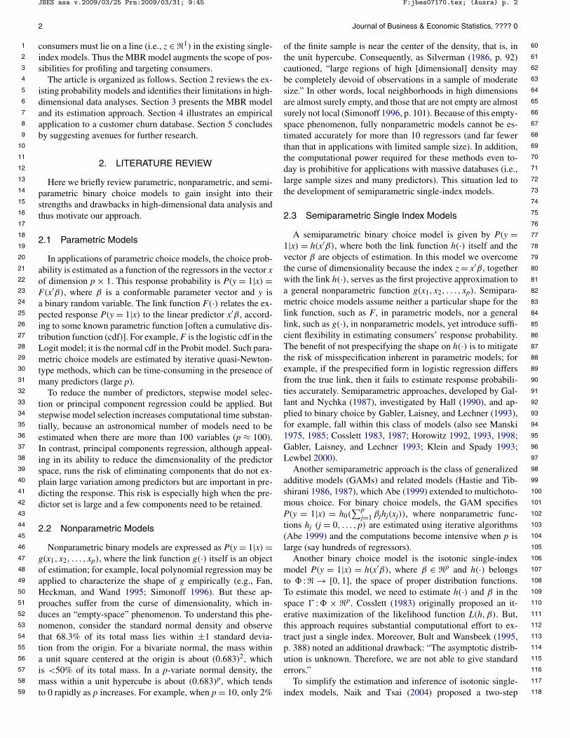
ij . After rounding off the estimates,we present the frequency of estimated power transforms in Fig-ure 1. We find that in this application, the logarithmic transformis valid for about half of the variables, whereas the square root(λ = 0.5) and linear (λ = 1) transforms are not the best choicesfor the other half. Thus the shapes of the distributions differwidely across variables, requiring different power transformsfor various regressors.

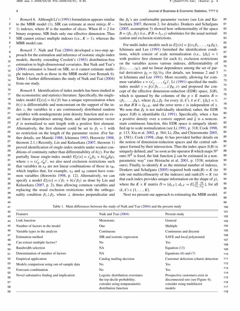
Does the transformation matter? To assess it, we apply eigen-decomposition in (2) to the data set with original and trans-formed regressors. Figure 2 displays the eigenplots for thefirst 50 out of 124 factors (for the sake of clarity). Compar-ing the two curves demonstrates a relatively sharper decline for

Naik, Wedel, and Kamakura: Multi-Index Binary Response Analysis of Large Data Sets

JBES asa v.2009/03/25 Prn:2009/03/31; 9:45 F:jbes07170.tex; (Ausra) p. 9

9

1 60

2 61

3 62

4 63

5 64

6 65

7 66

8 67

9 68

10 69

11 70

12 71

13 72

14 73

15 74

16 75

17 76

18 77

19 78

20 79

21 80

22 81

23 82

24 83

25 84

26 85

27 86

28 87

29 88

30 89

31 90

32 91

33 92

34 93

35 94

36 95

37 96

38 97

39 98

40 99

41 100

42 101

43 102

44 103

45 104

46 105

47 106

48 107

49 108

50 109

51 110

52 111

53 112

54 113

55 114

56 115

57 116

58 117

59 118

Figure 1. Frequency of estimated power transforms.

the transformed regressors. For example, for the transformedregressors, just 10 out of 104 eigenvalues exceed λ = 0.5,whereas it takes 25 factors to attain that cutoff (indicated by thedashed line) based on original regressors. Furthermore, a simi-lar result holds for every cutoff level (see Figure 2). Thus usingnonlinear transformations of the regressors compress greater in-formation into fewer factors (also see de Leeuw 2005, p. 8).

4.2.2 Number of Factors. Figure 2 further reveals that wecannot determine the number of factors to retain by eyeballingthe eigenplot of transformed regressors, because its gradientchanges smoothly (unlike the “scree plot” in principal compo-nent analysis). Thus we apply the permutation test and infor-mation criterion. Cook and Yin (2001, p. 155) developed thepermutation test based on resampling the data (see their propo-sition 2i for its theoretical basis). For this application, this in-dicates that we retain fewer than τ = 75 factors (i.e., the upperbound on the number of factors in the population). Next, basedon the information criterion of Zhu, Miao, and Peng (2006),we compute G(k) in (6) and present it in Figure 3. It showsthat G(k) attains the maximum value at K∗ = 4, and thus weretain the first four factors, which strike the optimal balance be-tween fit and parsimony.

This result raises three important points. First, we achieved amarked reduction in dimensionality from p = 124 regressors to

K∗ = 4 indexes (or factors) without prespecifying a particularlink function. Second, our data provide empirical evidence tosupport the need for more than a single index (i.e., K = 1) to de-scribe binary response variable, justifying the proposed multi-index binary response model. Finally, does substantial dimen-sion reduction lead to severe information loss relative to retain-ing all of the regressors, ceteris paribus (e.g., the link function)?We address this question in Section 4.3 using out-of-sampleforecasts.

4.2.3 Fitting Multivariate Link and Locating ProspectiveCustomers. Nonparametric estimation of g(·) would be prac-tically impossible using the original 124 regressors. However,having projected all of the regressors on a four-dimensionalsubspace, we can calibrate the churn probability P(Y = 1) =gb(Z1, Z2, Z3, Z4) nonparametrically. Toward this end, we ap-ply multivariate local polynomial regression of order 1 (i.e.,local linear), because even ordered fits (e.g., local constant orquadratic) reduce efficiency and suffer from boundary effects(see Fan and Gijbels 1996, p. 79). Specifically, we apply Equa-tion (12) to the four factor scores and binary response.

To select the bandwidth b, we evaluate the AIC-type infor-mation criterion in (13), modified to obtain a BIC-type criterionby replacing the penalty term by pb Ln(N). Table 3 presents the

Figure 2. Eigenplot for the first 50 factors.

JBES asa v.2009/03/25 Prn:2009/03/31; 9:45 F:jbes07170.tex; (Ausra) p. 10

10 Journal of Business & Economic Statistics, ???? 0

1 60

2 61

3 62

4 63

5 64

6 65

7 66

8 67

9 68

10 69

11 70

12 71

13 72

14 73

15 74

16 75

17 76

18 77

19 78

20 79

21 80

22 81

23 82

24 83

25 84

26 85

27 86

28 87

29 88

30 89

31 90

32 91

33 92

34 93

35 94

36 95

37 96

38 97

39 98

40 99

41 100

42 101

43 102

44 103

45 104

46 105

47 106

48 107

49 108

50 109

51 110

52 111

53 112

54 113

55 114

56 115

57 116

58 117

59 118

Figure 3. Factor determination using the information criterion.

AIC and BIC and the trace of the hat matrix for various band-widths. Note that the effective number of parameters (via thetrace) decreases as bandwidth increases; however, its impact onAICC and BIC is different. AICC increases with bandwidth be-cause tr(Qb) is small relative to the sample size N = 10,000,recommending that we select the smallest bandwidth; whereasBIC decreases with bandwidth because Ln(N) imposes a strongpenalty compared with the improvements in the model fit, indi-cating that we select a larger bandwidth. Given these oppositerecommendations, we compute b = 0.79σN−1/5, where σ isthe average range over the four factor scores (Z1, Z2, Z3, Z4),yielding the empirical bandwidth b = 7.2 for this sample.

Without assuming any functional form for g(·), we calibratethe link function using the closed-form estimator (12), the em-pirical bandwidth in (11), the four estimated factor scores, andthe binary response. The resulting link function helps us predictthe response probability for prospective customers (not just theexisting ones). Specifically, consider a prospective customer—not listed in the CRM database—located at an arbitrary pointt = (t1, t2, t3, t4)′ in a four-dimensional index space. The chancethat this prospective customer churns is given by g(t1, t2, t3, t4).By evaluating the churn probability for customers located in theregion t ∈ �4, we identify where high-risk prospects live.

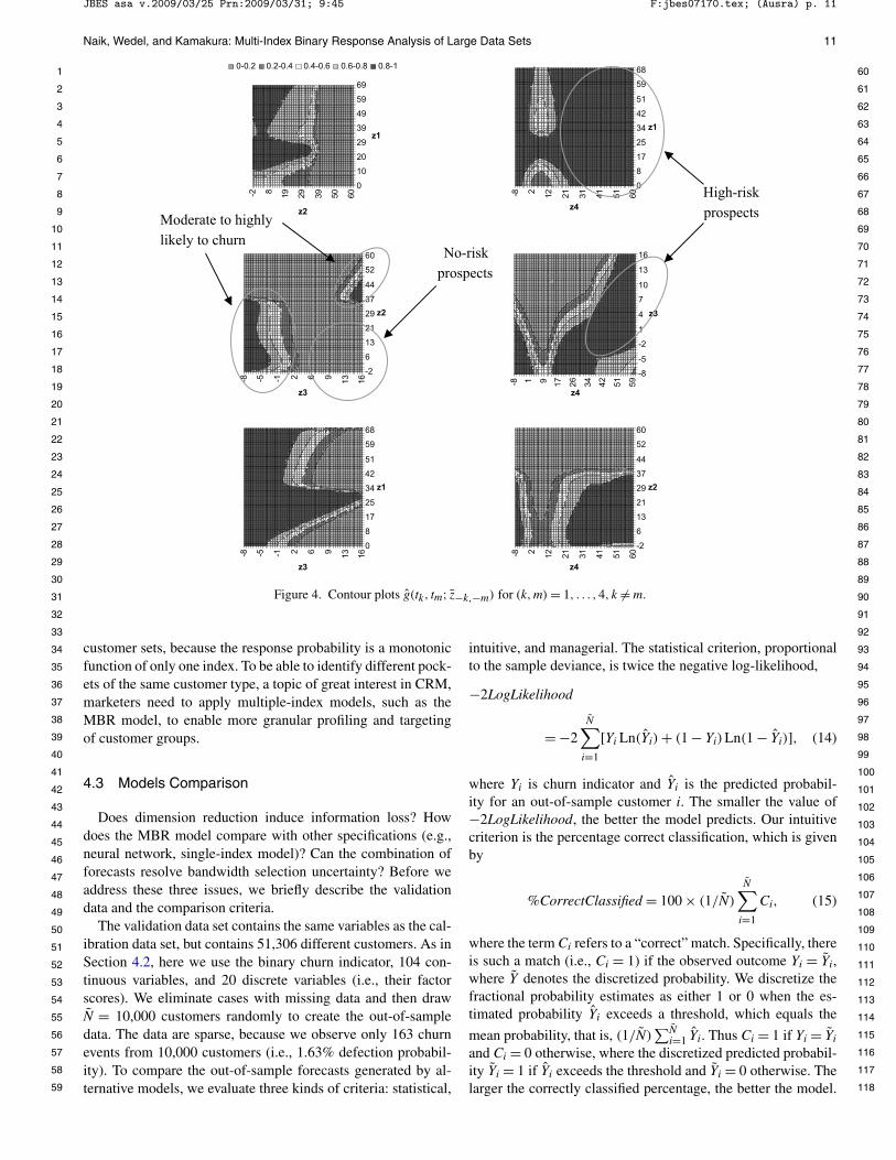
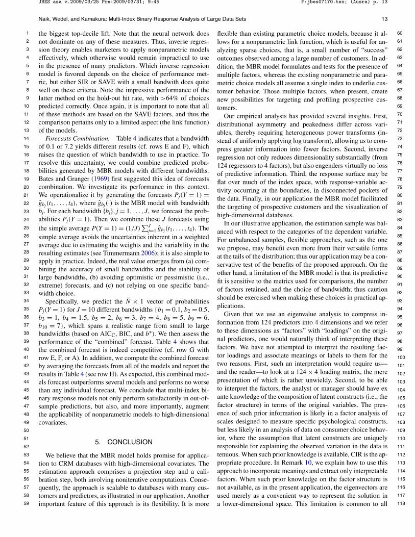
To locate high-risk prospects, we construct contour plotsof g(·) in two-dimensional spaces. Specifically, for a prospec-tive customers at any point (tk, tm) in two-factor space, werepresent similar values of g(tk, tm; z−k,−m) by a certain color,holding other factors fixed at their sample means (i.e., z−k,−m).Figure 4 depicts six contour plots resulting from the index com-binations (k,m) = 1, . . . ,4 and k = m. To aid customer iden-tification, we use color graphics to visualize the quintiles ofchurn probabilities: no-risk (<0.2), low-probability (0.2–0.4),medium-probability (0.4–0.6), high-probability (0.6–0.8), and

high-risk (>0.8) customers. Such a visualization is useful inpractical applications as well.

We glean four insights from these results. First, we observethat a vast landscape in four dimensions is nearly flat. This sug-gests that many prospective customers have churn probabilityclose to 0; they exhibit inertia perhaps due to contractual con-straints or product satisfaction. The good news is that we knowwho not to mail the retention promotions to proactively, andknow that this constitutes a large proportion of customers, thusleading to substantial savings and avoiding “overtouching” thecustomer with unnecessary mailings. The framework proposedby Bult and Wansbeek (1995) can be adapted to optimally se-lect customers at risk by maximizing profit based on this MBRmodel.

Second, our findings corroborate the results of Naik andTsai (2004), which show that the logistic distribution overesti-mates customers’ response probability. Estimating the unknownlink function by nonparametric methods (rather than prespeci-fied) not only mitigates misspecification errors, but also pro-motes a more conservative approach to database marketing.

Third, due to the empty-space phenomenon, customers arespread out in the edges of the high-dimensional space. Conse-quently, the support (or domain) of the estimated link functionexceeds the typical range of ±3 standard deviations (see Fig-ure 4). In other words, outliers are the norm rather than excep-tion.

Finally, we document evidence that high-risk customers be-long to disconnected sets in the four-dimensional latent space.Specifically, Figure 4 shows the sets of customers with no churnrisk, moderate churn risk, and high churn risk. Note that the setof moderately risky customers is not contiguous. Existing prob-ability models, regardless whether they fit parametric or non-parametric link functions, cannot identify such disconnected

Table 3. Information criteria and tr(Q) across bandwidths

Bandwidth, b AICC BIC Trace(Q)

0.05 23,475 15,201 2410.1 23,570 14,593 1430.5 23,760 14,080 451 23,804 14,006 282 23,816 13,955 205 23,826 13,917 13

10 23,832 13,901 10

Naik, Wedel, and Kamakura: Multi-Index Binary Response Analysis of Large Data Sets

JBES asa v.2009/03/25 Prn:2009/03/31; 9:45 F:jbes07170.tex; (Ausra) p. 11

11

1 60

2 61

3 62

4 63

5 64

6 65

7 66

8 67

9 68

10 69

11 70

12 71

13 72

14 73

15 74

16 75

17 76

18 77

19 78

20 79

21 80

22 81

23 82

24 83

25 84

26 85

27 86

28 87

29 88

30 89

31 90

32 91

33 92

34 93

35 94

36 95

37 96

38 97

39 98

40 99

41 100

42 101

43 102

44 103

45 104

46 105

47 106

48 107

49 108

50 109

51 110

52 111

53 112

54 113

55 114

56 115

57 116

58 117

59 118

Figure 4. Contour plots g(tk, tm; z−k,−m) for (k,m) = 1, . . . ,4, k = m.

customer sets, because the response probability is a monotonicfunction of only one index. To be able to identify different pock-ets of the same customer type, a topic of great interest in CRM,marketers need to apply multiple-index models, such as theMBR model, to enable more granular profiling and targetingof customer groups.

4.3 Models Comparison

Does dimension reduction induce information loss? Howdoes the MBR model compare with other specifications (e.g.,neural network, single-index model)? Can the combination offorecasts resolve bandwidth selection uncertainty? Before weaddress these three issues, we briefly describe the validationdata and the comparison criteria.

The validation data set contains the same variables as the cal-ibration data set, but contains 51,306 different customers. As inSection 4.2, here we use the binary churn indicator, 104 con-tinuous variables, and 20 discrete variables (i.e., their factorscores). We eliminate cases with missing data and then drawN = 10,000 customers randomly to create the out-of-sampledata. The data are sparse, because we observe only 163 churnevents from 10,000 customers (i.e., 1.63% defection probabil-ity). To compare the out-of-sample forecasts generated by al-ternative models, we evaluate three kinds of criteria: statistical,

intuitive, and managerial. The statistical criterion, proportionalto the sample deviance, is twice the negative log-likelihood,

−2LogLikelihood

= −2N∑

i=1

[Yi Ln(Yi) + (1 − Yi)Ln(1 − Yi)], (14)

where Yi is churn indicator and Yi is the predicted probabil-ity for an out-of-sample customer i. The smaller the value of−2LogLikelihood, the better the model predicts. Our intuitivecriterion is the percentage correct classification, which is givenby

%CorrectClassified = 100 × (1/N)

N∑

i=1

Ci, (15)

where the term Ci refers to a “correct” match. Specifically, thereis such a match (i.e., Ci = 1) if the observed outcome Yi = Yi,where Y denotes the discretized probability. We discretize thefractional probability estimates as either 1 or 0 when the es-timated probability Yi exceeds a threshold, which equals the

mean probability, that is, (1/N)∑N

i=1 Yi. Thus Ci = 1 if Yi = Yi

and Ci = 0 otherwise, where the discretized predicted probabil-ity Yi = 1 if Yi exceeds the threshold and Yi = 0 otherwise. Thelarger the correctly classified percentage, the better the model.

JBES asa v.2009/03/25 Prn:2009/03/31; 9:45 F:jbes07170.tex; (Ausra) p. 12

12 Journal of Business & Economic Statistics, ???? 0

1 60

2 61

3 62

4 63

5 64

6 65

7 66

8 67

9 68

10 69

11 70

12 71

13 72

14 73

15 74

16 75

17 76

18 77

19 78

20 79

21 80

22 81

23 82

24 83

25 84

26 85

27 86

28 87

29 88

30 89

31 90

32 91

33 92

34 93

35 94

36 95

37 96

38 97

39 98

40 99

41 100

42 101

43 102

44 103

45 104

46 105

47 106

48 107

49 108

50 109

51 110

52 111

53 112

54 113

55 114

56 115

57 116

58 117

59 118

The managerial criterion is the top decile lift (see Lemmens andCroux 2006, p. 280), which is given by the proportion of churn-ers in the top 10% of the sample (= π10%) divided by the pro-portion of churners in the entire validation sample (= π100%),

TopDecile = π10%

π100%. (16)

The greater the lift, the better the model predicts. Top decile liftfocuses on “prime” customers because companies target theirmarketing efforts at this subgroup, thus affecting their profits(see Neslin et al. 2006). When it equals unity, the model has nopredictive power, because the targeted customers are as likelyto churn as the rest of the sample. But although this criterionis used frequently in practice, we attribute less weight to it, be-cause, unlike the other two criteria, it ignores the accuracy ofa classifier across the remaining 90% of the sample and is mis-leading for models that overestimate the top decile probability(as noted in Naik and Tsai 2004). Next we address the threeissues that we raised earlier.

Information Loss. We compare the accuracy of out-of-sample forecasts when the forecasting model uses informationcontained in the 4 SAVE factors versus all 124 regressors ceterisparibus, i.e., keeping the link function the same. The SAVE fac-tors are obtained by combining the values of the 124 regressorsin the validation data with the factor loadings obtained from theestimation sample. We apply logistic regression to the calibra-tion data and estimate the model parameters, which we combinewith the regressors (or four SAVE factors) from the validationdata to predict the out-of-sample probability, Y = P(Y = 1). Inother words, we do not use the actual churn indicator Y in thevalidation sample to estimate the model parameters, and thusour model comparisons are based on true predictions.

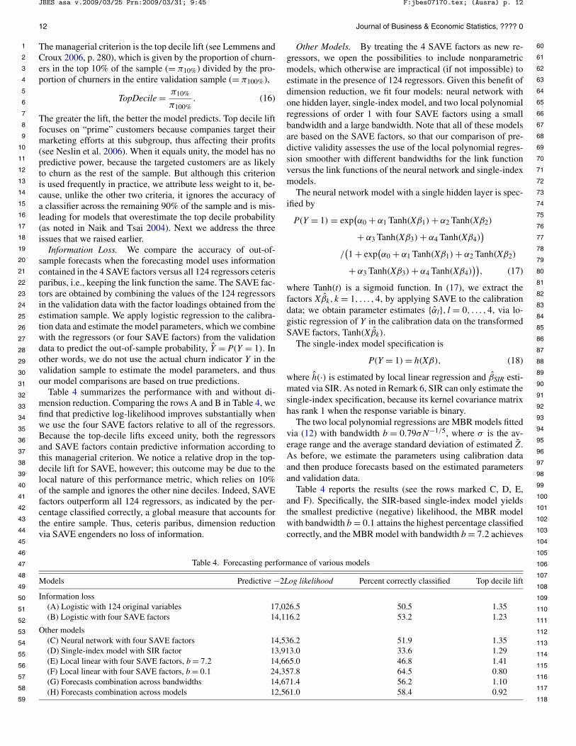
Table 4 summarizes the performance with and without di-mension reduction. Comparing the rows A and B in Table 4, wefind that predictive log-likelihood improves substantially whenwe use the four SAVE factors relative to all of the regressors.Because the top-decile lifts exceed unity, both the regressorsand SAVE factors contain predictive information according tothis managerial criterion. We notice a relative drop in the top-decile lift for SAVE, however; this outcome may be due to thelocal nature of this performance metric, which relies on 10%of the sample and ignores the other nine deciles. Indeed, SAVEfactors outperform all 124 regressors, as indicated by the per-centage classified correctly, a global measure that accounts forthe entire sample. Thus, ceteris paribus, dimension reductionvia SAVE engenders no loss of information.

Other Models. By treating the 4 SAVE factors as new re-gressors, we open the possibilities to include nonparametricmodels, which otherwise are impractical (if not impossible) toestimate in the presence of 124 regressors. Given this benefit ofdimension reduction, we fit four models: neural network withone hidden layer, single-index model, and two local polynomialregressions of order 1 with four SAVE factors using a smallbandwidth and a large bandwidth. Note that all of these modelsare based on the SAVE factors, so that our comparison of pre-dictive validity assesses the use of the local polynomial regres-sion smoother with different bandwidths for the link functionversus the link functions of the neural network and single-indexmodels.

The neural network model with a single hidden layer is spec-ified by

P(Y = 1) = exp(α0 + α1 Tanh(Xβ1) + α2 Tanh(Xβ2)

+ α3 Tanh(Xβ3) + α4 Tanh(Xβ4))

/(1 + exp

(α0 + α1 Tanh(Xβ1) + α2 Tanh(Xβ2)

+ α3 Tanh(Xβ3) + α4 Tanh(Xβ4)))

, (17)

where Tanh(t) is a sigmoid function. In (17), we extract thefactors Xβk, k = 1, . . . ,4, by applying SAVE to the calibrationdata; we obtain parameter estimates {αl}, l = 0, . . . ,4, via lo-gistic regression of Y in the calibration data on the transformedSAVE factors, Tanh(Xβk).

The single-index model specification is

P(Y = 1) = h(Xβ), (18)

where h(·) is estimated by local linear regression and βSIR esti-mated via SIR. As noted in Remark 6, SIR can only estimate thesingle-index specification, because its kernel covariance matrixhas rank 1 when the response variable is binary.

The two local polynomial regressions are MBR models fittedvia (12) with bandwidth b = 0.79σN−1/5, where σ is the av-erage range and the average standard deviation of estimated Z.As before, we estimate the parameters using calibration dataand then produce forecasts based on the estimated parametersand validation data.

Table 4 reports the results (see the rows marked C, D, E,and F). Specifically, the SIR-based single-index model yieldsthe smallest predictive (negative) likelihood, the MBR modelwith bandwidth b = 0.1 attains the highest percentage classifiedcorrectly, and the MBR model with bandwidth b = 7.2 achieves

Table 4. Forecasting performance of various models

Models Predictive −2Log likelihood Percent correctly classified Top decile lift

Information loss(A) Logistic with 124 original variables 17,026.5 50.5 1.35(B) Logistic with four SAVE factors 14,116.2 53.2 1.23

Other models(C) Neural network with four SAVE factors 14,536.2 51.9 1.35(D) Single-index model with SIR factor 13,913.0 33.6 1.29(E) Local linear with four SAVE factors, b = 7.2 14,665.0 46.8 1.41(F) Local linear with four SAVE factors, b = 0.1 24,357.8 64.5 0.80(G) Forecasts combination across bandwidths 14,671.4 56.2 1.10(H) Forecasts combination across models 12,561.0 58.4 0.92

Naik, Wedel, and Kamakura: Multi-Index Binary Response Analysis of Large Data Sets

JBES asa v.2009/03/25 Prn:2009/03/31; 9:45 F:jbes07170.tex; (Ausra) p. 13

13

1 60

2 61

3 62

4 63

5 64

6 65

7 66

8 67

9 68

10 69

11 70

12 71

13 72

14 73

15 74

16 75

17 76

18 77

19 78

20 79

21 80

22 81

23 82

24 83

25 84

26 85

27 86

28 87

29 88

30 89

31 90

32 91

33 92

34 93

35 94

36 95

37 96

38 97

39 98

40 99

41 100

42 101

43 102

44 103

45 104

46 105

47 106

48 107

49 108

50 109

51 110

52 111

53 112

54 113

55 114

56 115

57 116

58 117

59 118

the biggest top-decile lift. Note that the neural network doesnot dominate on any of these measures. Thus, inverse regres-sion theory enables marketers to apply nonparametric modelseffectively, which otherwise would remain impractical to usein the presence of many predictors. Which inverse regressionmodel is favored depends on the choice of performance met-ric, but either SIR or SAVE with a small bandwith does quitewell on these criteria. Note the impressive performance of thelatter method on the hold-out hit rate, with >64% of choicespredicted correctly. Once again, it is important to note that allof these methods are based on the SAVE factors, and thus thecomparison pertains only to a limited aspect (the link function)of the models.

Forecasts Combination. Table 4 indicates that a bandwidthof 0.1 or 7.2 yields different results (cf. rows E and F), whichraises the question of which bandwidth to use in practice. Toresolve this uncertainty, we could combine predicted proba-bilities generated by MBR models with different bandwidths.Bates and Granger (1969) first suggested this idea of forecastscombination. We investigate its performance in this context.We operationalize it by generating the forecasts Pj(Y = 1) =gbj(t1, . . . , t4), where gbj(·) is the MBR model with bandwidthbj. For each bandwidth {bj}, j = 1, . . . , J, we forecast the prob-abilities Pj(Y = 1). Then we combine these J forecasts usingthe simple average P(Y = 1) = (1/J)

∑Jj=1 gbj(t1, . . . , t4). The

simple average avoids the uncertainties inherent in a weightedaverage due to estimating the weights and the variability in theresulting estimates (see Timmermann 2006); it is also simple toapply in practice. Indeed, the real value emerges from (a) com-bining the accuracy of small bandwidths and the stability oflarge bandwidths, (b) avoiding optimistic or pessimistic (i.e.,extreme) forecasts, and (c) not relying on one specific band-width choice.

Specifically, we predict the N × 1 vector of probabilitiesPj(Y = 1) for J = 10 different bandwidths {b1 = 0.1, b2 = 0.5,b3 = 1, b4 = 1.5, b5 = 2, b6 = 3, b7 = 4, b8 = 5, b9 = 6,b10 = 7}, which spans a realistic range from small to largebandwidths (based on AICC, BIC, and b∗). We then assess theperformance of the “combined” forecast. Table 4 shows thatthe combined forecast is indeed competitive (cf. row G withrow E, F, or A). In addition, we compute the combined forecastby averaging the forecasts from all of the models and report theresults in Table 4 (see row H). As expected, this combined mod-els forecast outperforms several models and performs no worsethan any individual forecast. We conclude that multi-index bi-nary response models not only perform satisfactorily in out-of-sample predictions, but also, and more importantly, augmentthe applicability of nonparametric models to high-dimensionalcovariates.

5. CONCLUSION

We believe that the MBR model holds promise for applica-tion to CRM databases with high-dimensional covariates. Theestimation approach comprises a projection step and a cali-bration step, both involving noniterative computations. Conse-quently, the approach is scalable to databases with many cus-tomers and predictors, as illustrated in our application. Anotherimportant feature of this approach is its flexibility. It is more

flexible than existing parametric choice models, because it al-lows for a nonparametric link function, which is useful for an-alyzing sparse choices, that is, a small number of “success”outcomes observed among a large number of customers. In ad-dition, the MBR model formulates and tests for the presence ofmultiple factors, whereas the existing nonparametric and para-metric choice models all assume a single index to underlie cus-tomer behavior. Those multiple factors, when present, createnew possibilities for targeting and profiling prospective cus-tomers.

Our empirical analysis has provided several insights. First,distributional asymmetry and peakedness differ across vari-ables, thereby requiring heterogeneous power transforms (in-stead of uniformly applying log transform), allowing us to com-press greater information into fewer factors. Second, inverseregression not only reduces dimensionality substantially (from124 regressors to 4 factors), but also engenders virtually no lossof predictive information. Third, the response surface may beflat over much of the index space, with response-variable ac-tivity occurring at the boundaries, in disconnected pockets ofthe data. Finally, in our application the MBR model facilitatedthe targeting of prospective customers and the visualization ofhigh-dimensional databases.

In our illustrative application, the estimation sample was bal-anced with respect to the categories of the dependent variable.For unbalanced samples, flexible approaches, such as the onewe propose, may benefit even more from their versatile formsat the tails of the distribution; thus our application may be a con-servative test of the benefits of the proposed approach. On theother hand, a limitation of the MBR model is that its predictivefit is sensitive to the metrics used for comparisons, the numberof factors retained, and the choice of bandwidth; thus cautionshould be exercised when making these choices in practical ap-plications.

Given that we use an eigenvalue analysis to compress in-formation from 124 predictors into 4 dimensions and we referto these dimensions as “factors” with “loadings” on the origi-nal predictors, one would naturally think of interpreting thesefactors. We have not attempted to interpret the resulting fac-tor loadings and associate meanings or labels to them for thetwo reasons. First, such an interpretation would require us—and the reader—to look at a 124 × 4 loading matrix, the merepresentation of which is rather unwieldy. Second, to be ableto interpret the factors, the analyst or manager should have exante knowledge of the composition of latent constructs (i.e., thefactor structure) in terms of the original variables. The pres-ence of such prior information is likely in a factor analysis ofscales designed to measure specific psychological constructs,but less likely in an analysis of data on consumer choice behav-ior, where the assumption that latent constructs are uniquelyresponsible for explaining the observed variation in the data istenuous. When such prior knowledge is available, CIR is the ap-propriate procedure. In Remark 10, we explain how to use thisapproach to incorporate meanings and extract only interpretablefactors. When such prior knowledge on the factor structure isnot available, as in the present application, the eigenvectors areused merely as a convenient way to represent the solution ina lower-dimensional space. This limitation is common to all

JBES asa v.2009/03/25 Prn:2009/03/31; 9:45 F:jbes07170.tex; (Ausra) p. 14

14 Journal of Business & Economic Statistics, ???? 0

1 60

2 61

3 62

4 63

5 64

6 65

7 66

8 67

9 68

10 69

11 70

12 71

13 72

14 73

15 74

16 75

17 76

18 77

19 78

20 79

21 80

22 81

23 82

24 83

25 84

26 85

27 86

28 87

29 88

30 89

31 90

32 91

33 92

34 93

35 94

36 95

37 96

38 97

39 98

40 99

41 100

42 101

43 102

44 103

45 104

46 105

47 106

48 107

49 108

50 109

51 110

52 111

53 112

54 113

55 114

56 115

57 116

58 117

59 118

factor-analytic methods that lack ex ante knowledge of the la-tent factor structures, as is generally the case in applications torevealed preference data.

In summary, this study not only broadens the scope of binarychoice models to embrace nonlinear, nonparametric, multifac-tor models in the presence of many predictors, but also providesa practical and computationally feasible approach for estimat-ing factor scores, determining the number of factors, calibrat-ing the nonlinear link function, selecting the bandwidth, andcombining out-of-sample forecasts. We conclude by suggestingthree avenues for further research:

• Alternative transformations. Figure 2 shows that we canconcentrate more information into fewer factors whenwe attain normality, which we achieve through univariatepower transformation of each regressor. Alternatively, wecould attain multivariate normality through the approachof Velilla (1993). Similarly, through the approach of Cookand Nachtsheim (1994), we could induce more general el-liptically contoured distributions for the regressors ratherthan restricting them to be normal. Future research mayinvestigate the costs and benefits of these alternative trans-formations.

• Asymptotic distribution of factor loadings. We derived theasymptotic distribution of factor loadings of SAVE to ob-tain a new result, which can be used to conduct statisticalinference on factor loadings in applied research. However,to apply this result, future studies need to construct a con-sistent estimator of �Q.

• Multivariate response. The MBR model predicts a sin-gle transaction, for example, the churn indicator, whichis a single Y variable. Its extension to multiple correlatedresponse variables is of substantial interest, because thiswould enable companies to improve their cross-selling ef-forts across multiple products and services (Kamakura etal. 2003). Toward this end, future research could apply theideas in “Alternating SIR,” developed by Li et al. (2003),which reduces the dimensionality of both Y ∈ �m and X ∈�p simultaneously without specifying the vector-valuedlink functions. An analysis similar to alternating SIR, butthrough the kernel matrix from SAVE, would facilitate theinclusion of multiple response variables in MBR models.

We hope that this study marks a useful starting point for fur-ther development and that it stimulates researchers to join in theeffort to advance the theory and practice of high-dimensionaldata analyses.

ACKNOWLEDGMENTS

The first two authors appreciate the financial support of theTeradata Center at Duke University for this research. The au-thors acknowledge that the Editor, Area Editor, and the review-ers provided constructive comments, which improved the man-uscript.

[Received July 2007. Revised January 2008.]

REFERENCES

Abe, M. (1999), “A Generalized Additive Model for Discrete Choice Data,”Journal of Business and Economic Statistics, 17 (3), 271–284.

Bai, J., and Ng, S. (2002), “Determining the Number of Factors in ApproximateFactor Models,” Econometrica, 70 (1), 191–221.

Basilevsky, A. (1994), Statistical Factor Analysis and Related Methods: Theoryand Applications, New York: Wiley.

Bates, J. M., and Granger, C. W. J. (1969), “The Combination of Forecasts,”Operations Research Quarterly, 20, 451–468.

Bult, J. R., and Wansbeek, T. (1995), “Optimal Selection for Direct Mail,” Mar-keting Science, 14 (4), 378–394.

Chen, C.-H., and Li, K.-C. (1998), “Can SIR Be as Popular as Multiple LinearRegression?” Statistica Sinica, 8, 289–316.

Chiaromonte, F., Cook, R. D., and Li, B. (2002), “Sufficient Dimension Reduc-tion in Regressions With Categorical Predictors,” The Annals of Statistics,30 (2), 475–497.

Cook, R. D. (1998), Regression Graphics: Ideas for Studying RegressionsThrough Graphics, New York: Wiley.

Cook, R. D., and Lee, H. (1999), “Dimension Reduction in Binary ResponseModels,” Journal of the American Statistical Association, 94 (448), 1187–1200.

Cook, R. D., and Nachtsheim, C. J. (1994), “Reweighting to Achieve Ellipti-cally Contoured Covariates in Regression,” Journal of the American Statis-tical Association, 89 (426), 592–599.

Cook, R. D., and Weisberg, S. (1991), Discussion on “Sliced Inverse Regressionfor Dimension Reduction,” by K.-C. Li, Journal of the American StatisticalAssociation, 86, 328–332.

Cook, R. D., and Yin, X. (2001), “Dimension Reduction and Visualization inDiscriminant Analysis” (with discussion), Australian & New Zealand Jour-nal of Statistics, 43 (2), 147–199.

Cosslett, S. R. (1983), “Distribution-Free Maximum Likelihood Estimator ofthe Binary Choice Model,” Econometrica, 51, 765–782.

(1987), “Efficiency Bounds for Distribution-Free Maximum Likeli-hood Estimator of the Binary Choice and Censored Regression Models,”Econometrica, 55, 559–585.

Day, G. S. (2000), “Capabilities for Forging Customer Relations,” Working Pa-per 00-118, MSI, Cambridge, MA.

De Leeuw, J. (2005), “Nonlinear Principal Components Analysis and RelatedTechniques,” eScholarship Repository, University of California, available athttp:// repositories.cdlib.org/uclastat/papers/20005070801.

Donkers, B., and Schafgans, M. (2005), “A Method of Moments Estimator forSemiparametric Index Models,” Working Paper EM/05/493.

Fan, J. (1992), “Design-Adaptive Nonparametric Regression,” Journal of theAmerican Statistical Association, 87 (420), 998–1004.

Fan, J., and Gijbels, I. (1996), Local Polynomial Modeling and Its Applications,Suffolk: Chapman & Hall.

Fan, J. Q., Heckman, N. E., and Wand, M. P. (1995), “Local Polynomial Ker-nel Regression for Generalized Linear Models and Quasi-Likelihood Func-tions,” Journal of the American Statistical Association, 90, 141–150.

Gabler, S., Laisney, F., and Lechner, M. (1993), “Semi-Nonparametric Estima-tion of Binary Choice Models With an Application to Labor-Force Partici-pation,” Journal of Business and Economic Statistics, 11 (1), 61–80.

Gallant, A. R., and Nychka, D. N. (1987), “Semi-Nonparametric MaximumLikelihood Estimation,” Econometrica, 57, 1091–1120.

Gifi, A. (1990), Nonlinear Multivariate Analysis, Chichester, U.K.: Wiley.Hall, A. (1990), “Lagrange Multiplier Test for Normality Against Seminon-

parametric Alternatives,” Journal of Business and Economic Statistics, 8,417–426.

Hardle, W., and Stoker, T. M. (1989), “Investigating Smooth Multiple Regres-sion by the Method of Average Derivatives,” Journal of the American Sta-tistical Association, 84, 986–995.

Hastie, T. R., and Tibshirani, R. (1986), “Generalized Additive Models: SomeApplications,” Journal of the American Statistical Association, 82, 371–386.

(1987), “Generalized Additive Models,” Statistical Science, 1, 197–318.

Horowitz, J. L. (1992), “A Smoothed Maximum Score Estimator for the BinaryResponse Model,” Econometrica, 60, 505–531.

(1993), “Optimal Rates of Convergence of Parameter Estimators in theBinary Response Model With Weak Distributional Assumptions,” Econo-metric Theory, 9, 1–18.

(1998), Semiparametric Methods in Econometrics, New York:Springer.

Hristache, M., Juditsky, A., Polzehl, J., and Spokoiny, V. (2001), “StructureAdaptive Approach for Dimension Reduction,” The Annals of Statistics,29 (6), 1537–1566.

Ichimura, H. (1993), “Semiparametric Least Squares (SLS) and Weighted SLDEstimation of Single-Index Models,” Journal of Econometrics, 58, 71–120.

Naik, Wedel, and Kamakura: Multi-Index Binary Response Analysis of Large Data Sets

JBES asa v.2009/03/25 Prn:2009/03/31; 9:45 F:jbes07170.tex; (Ausra) p. 15

15

1 60

2 61

3 62

4 63

5 64

6 65

7 66

8 67

9 68

10 69

11 70

12 71

13 72

14 73

15 74

16 75

17 76

18 77

19 78

20 79

21 80

22 81

23 82

24 83

25 84

26 85

27 86

28 87

29 88

30 89

31 90

32 91

33 92

34 93

35 94

36 95

37 96

38 97

39 98

40 99

41 100

42 101

43 102

44 103

45 104

46 105

47 106

48 107

49 108

50 109

51 110

52 111

53 112

54 113

55 114

56 115

57 116

58 117

59 118

Ichimura, H., and Lee, L.-F. (1991), “Semiparametric Least Squares Estima-tion of Multiple Index Models: Single Equation Estimation,” in Nonpara-metric and Semiparametric Methods in Econometrics and Statistics, eds.W. A. Barnett, J. Powell, and G. Tauchen, Cambridge: Cambridge Univer-sity Press, Chap. 1.

Kamakura, W., de Rosa, F., Wedel, M., and Mazzon, J. A. (2003), “Cross-Selling Financial Services With Database Marketing,” International Jour-nal of Research in Marketing, 20 (1), 45–65.

Kato, T. (1995), Perturbation Theory for Linear Operators, Berlin: Springer-Verlag.

Klein, R. W., and Spady, R. H. (1993), “An Efficient Semiparametric Estimatorfor Binary Response Models,” Econometrica, 61 (2), 387–421.

Lemmens, A., and Croux, C. (2006), “Bagging and Boosting ClassificationTrees to Predict Churn,” Journal of Marketing Research, 43 (2), 276–286.

Lewbel, A. (2000), “Semiparametric Qualitative Response Model EstimationWith Unknown Heteroscedasticity and Instrumental Variables,” Journal ofEconometrics, 97, 145–177.

Li, B., Zha, H., and Chiaromonte, F. (2005), “Contour Regression: A GeneralApproach to Dimension Reduction,” The Annals of Statistics, 33 (4), 1580–1616.

Li, K.-C. (1991), “Sliced Inverse Regression for Dimension Reduction,” Jour-nal of the American Statistical Association, 86, 316–342.

Li, K.-C., Aragon, Y., Shedden, K., and Agnan, C. T. (2003), “Dimension Re-duction for Multivariate Response Data,” Journal of the American Statisti-cal Association, 98 (461), 99–109.

Li, Y., and Zhu, L. (2006), “Asymptotics for Sliced Average Variance Estima-tion,” The Annals of Statistics, 35, 41–69.

Lin, W., and Kulasekara, K. B. (2007), “Idenitifiability of Single-Index Modelsand Additive-Index Models,” Biometrika, 1–6.

Manski, C. F. (1975), “Maximum Score Estimator of the Stochastic UtilityModel of Choice,” Journal of Econometrics, 3, 205–228.

(1985), “Semiparametric Analysis of Discrete Response: AsymptoticProperties of the Maximum Score Estimator,” Journal of Econometrics, 27,313–333.

(1988), “Identification of Binary Response Models,” Journal of theAmerican Statistical Association, 83, 729–738.

Naik, P. A., and Tsai, C.-L. (2001), “Single-Index Model Selections,” Bio-metrika, 88 (3), 821–832.

(2004), “Isotonic Single-Index Model for Database Marketing,” Com-putational Statistics and Data Analysis, to appear.

(2005), “Constrained Inverse Regression for Incorporating Prior Infor-mation,” Journal of the American Statistical Association, 100 (469), 204–211.

Neslin, S., Gupta, S., Kamakura, W., Lu, J., and Mason, C. (2006) “DefectionDetection: Measuring and Understanding the Predictive Accuracy of Cus-tomer Churn Models,” Journal of Marketing Research, 43 (2), 204–211.

Pagan, A., and Ullah, A. (1999), Nonparametric Econometrics, New York:Cambridge University Press.

Samarov, A. M. (1993), “Exploring Regression Structure Using NonparametricFunctional Estimation,” Journal of the American Statistical Association, 88,836–847.

Silverman, B. W. (1986), Density Estimation, London: Chapman & Hall.Simonoff, J. S. (1996), Smoothing Methods in Statistics, New York: Springer.Stock, J. H., and Watson, M. W. (2006), “Forecasting With Many Predictors,” in

Handbook of Economic Forecasting, Vol. 1, eds. G. Elliott, C. W. J. Granger,and A. Timmermann, Elsevier, Chap. 10.

Timmermann, A. (2006), “Forecast Combinations,” in Handbook of EconomicForecasting, Vol. 1, eds. G. Elliott, C. W. J. Granger, and A. Timmermann,Elsevier, pp. 135–196.

Tyler, D. E. (1981), “Asymptotic Inference for Eigenvectors,” The Annals ofStatistics, 9 (4), 725–736.

Velilla, S. (1993), “A Note on Multivariate Box–Cox Transformations to Nor-mality,” Statistics and Probability Letters, 17, 315–322.

Winer, R. S. (2001), “A Framework for Customer Relationship Management,”California Management Review, 43 (4), 89–105.

Xia, Y., Tong, H., Li, W. K., and Zhu, L.-X. (2002), “An Adaptive Estimationof Dimension Reduction Space,” Journal of the Royal Statistical Society,Ser. B, 64 (3), 363–410.

Zhu, L., Miao, B., and Peng, H. (2006), “On Sliced Inverse Regression WithHigh-Dimensional Covariates,” Journal of the American Statistical Associ-ation, 101 (474), 630–643.

JBES asa v.2009/03/25 Prn:2009/03/31; 9:45 F:jbes07170.tex; (Ausra) p. 16

1 1

2 2

3 3

4 4

5 5

6 6

7 7

8 8

9 9

10 10

11 11

12 12

13 13

14 14

15 15

16 16

17 17

18 18

19 19

20 20

21 21

22 22

23 23

24 24

25 25

26 26

27 27

28 28

29 29

30 30

31 31

32 32

33 33

34 34

35 35

36 36

37 37

38 38

39 39

40 40

41 41

42 42

43 43

44 44

45 45

46 46

47 47

48 48

49 49

50 50

51 51

52 52

53 53

54 54

55 55

56 56

57 57

58 58

59 59

META DATA IN THE PDF FILE

Following information will be included as pdf file Document Properties:

Title : Multi-Index Binary Response Analysisof Large Data SetsAuthor : Prasad A. Naik, Michel Wedel, Wagner KamakuraSubject : Journal of Business \046 Economic Statistics, Vol.0, No.00, 0, 1-16Keywords: Customer relationship marketing, Discrete choice, Factor model, Inverse regression, Semiparametric

estimation, Sliced average variance estimation

THE LIST OF URI ADRESSES

Listed below are all uri addresses found in your paper. The non-active uri addresses, if any, are indicated as ERROR. Please check and update the listwhere necessary. The e-mail addresses are not checked – they are listed just for your information. More information can be found in the support page:http://www.e-publications.org/ims/support/urihelp.html.

--- mailto:panaik@ucdavis.edu [2:pp.1,1] Check skip200 http://www.amstat.org [2:pp.1,1] OK302 http://pubs.amstat.org/loi/jbes [2:pp.1,1] Found200 http://dx.doi.org/10.1198/jbes.????.???? [2:pp.1,1] OK404 http://repositories.cdlib.org/uclastat/papers/20005070801 [2:pp.14,14] Not Found